Johnson–Holmquist-II(JH-2) Constitutive Model for Rock Materials: Parameter Determination and Application in Tunnel Smooth Blasting

Abstract

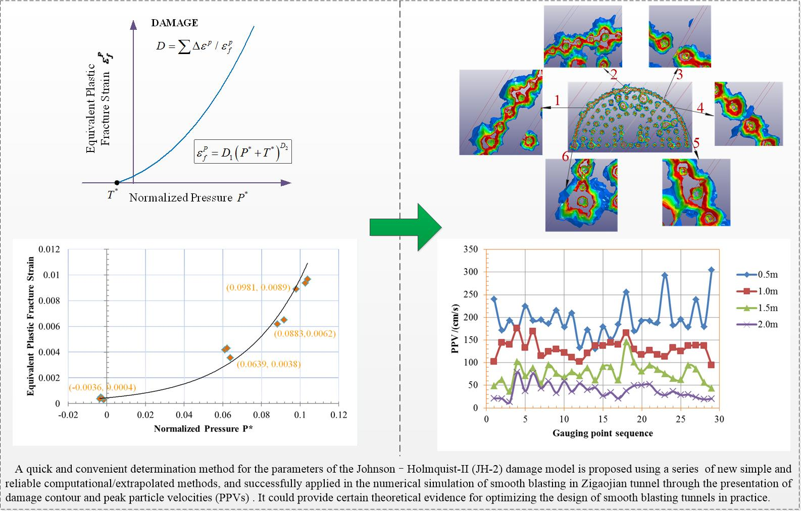
The Johnson–Holmquist-II(JH-2) model is introduced as the constitutive model for rock materials in tunnel smooth blasting. However, complicated and/or high-cost experiments need to be carried out to obtain the parameters of the JH-2 constitutive model. This study chooses Barre granite as an example to propose a quick and convenient determination method for the parameters of the JH-2 model using a series of computational and extrapolated methods. The validity of the parameters is verified via comparing the results of 3D numerical simulations with laboratory blast-loading experiments. Subsequently, the verified parameter determination method, together with the JH-2 damage constitutive model, is applied in the numerical simulation of smooth blasting in Zigaojian tunnel, Hangzhou–Huangshan high-speed railway. The overbreak/underbreak induced by rock blasting and joints/discontinuities is well estimated through comparing the damage contours resulting from the numerical study with the tunnel profiles measured from the tunnel site. The peak particle velocities (PPVs) of the near field are extracted to estimate the damage scope and damage degree for the surrounding rock mass of the tunnel on the basis of PPV damage criteria. This method can be used in the excavation of rock tunnels subjected to large strains, high strain rates, and high pressures, thereby reducing safety risk and economic losses.

1. Introduction

The material constitutive relationship is not only the conclusion of some regulations summarized from experimental data, but also plays an important role in numerical simulations. It reflects the realistic physical and mechanical properties of materials as much as possible to improve the accuracy of numerical results. At present, various kinds of constitutive models for materials are being developed and being optimized constantly along with an increasing need for numerical simulations. Especially for those materials under the loading conditions of large strains, high strain rates, and high pressures (LHH), dynamic constitutive models usually contain more complicated parameters of physical properties and some sensitive coefficients such as various rate effects [1,2,3,4,5] and strength coefficients [6,7,8], so that the parameter determination becomes an increasingly difficult problem. Therefore, accurate parameter determination for material constitutive models, which may directly affect the reliability and validity of the analytical results in numerical simulations, has become a significant task [9], and a growing number of researchers have devoted themselves to this work [10,11,12].

In computational constitutive models for materials subjected to LHH, Johnson, Cook, and Holmquist et al. contributed significantly to research on a wide variety of materials in the past 30 years. Initially, Johnson and Cook [1] reported a constitutive model and experimental data for metals including copper, brass, nickel, iron, etc., under LHH conditions. Later, the Johnson–Holmquist-Ceramics (JH-1) constitutive model was first presented by Johnson and Holmquist [2] to study the mechanical behavior of brittle materials subjected to LHH. Afterwards, a corrected constitutive model named the Johnson–Holmquist-2(JH-2) model [3] was presented based on the JH-1 model considering the softening property for some brittle materials such as boron carbide (B₄C). Further studies were performed for the high strain rate properties and constitutive modeling of glass [13] and the response of B₄C [4] subjected to severe loading conditions with LHH based on the JH-2 model, and subsequently a variety of impact and penetration problems were illustrated using the methods of Lagrangian finite element and Eulerian finite difference computations. During the same period, another constitutive model was developed for concrete subjected to LHH [14], called “HJC”, derived from the “Holmquist–Johnson–Cook” constitutive model [15,16]. Subsequently, Holmquist et al. [17] and Johnson et al. [5] expanded the application to aluminum nitride subjected to LHH using the JH-2 model. Different from the general brittle material, however, phase change is not considered in the previous JH-2 model, but is a new feature in their corrected constitutive model so that the embryonic form of the Johnson–Holmquist–Beissel (JHB) model was developed [5]. Additionally, Holmquist and Johnson [18,19] redressed the response of B₄C to high-velocity impact adopting optimized experimental data, and then the JHB constitutive model was used to simulate the material behavior under penetration, which illustrated the importance of the material parameters for the accuracy of simulations. Recently, a corrected computational constitutive model was presented based on the JHB model for glass subjected to LHH, and the effect of the third invariant was also included [20]. Apart from the JH-series constitutive models mentioned above, some novel constitutive models have also appeared considering different aspects, e.g., discontinuous deformation analysis (DDA) contact constitutive model [21], statistical damage constitutive model [22,23,24], average strain energy density (ASED) criterion for brittle and quasi-brittle materials [25], local and nonlocal damage models [6], frictional sliding crack model, and the strain energy density factor approach [7].

In the last decade, the JH-series constitutive models have begun to be used in the research of rock materials involving the excavation of mining, tunnels, and quarries. Ai and Ahrens [26] simulated shock-induced damage in granite targets impacted by projectiles at different velocities using the JH-2 model. Additionally, Ma and An [27], Wei et al. [28], Banadaki and Mohanty [29,30], and He and Yang [31] simulated stress-wave-induced fracture in granite due to explosive action using the JH-2 model, and then compared the crack patterns and pressures with lab-scale blast experiments and empirical formulae. However, the simulation methodologies above still remained in two dimensions, which may limit the total presentation for the transmission of stress waves and affect the final blasting results. Xia et al. [32] thus reproduced the rock dynamic fracture process of tunnel boring machine (TBM) tunneling in three dimensions. Moreover, the rock constitutive model was improved based on the JH-2 model by combing a Rankine tensile cracking softening model, however the validity of the improved model still needs to be deeply verified if employed in blasting rock tunnels. Li et al. [33,34] incorporated the JHB model into the particle-based numerical manifold method (PNMM) to study the dynamic behavior of rock blasting by dual-level discretization system. However, the computational method is generally used to simulate single borehole blasting under dynamic loading conditions; if employed in large-scale and three-dimensional modeling, it would be hard to complete because of the limitation of the PNMM algorithm. Gharehdash et al. [35] proposed a coupled finite element method (FEM) and smoothed particle hydrodynamics (SPH) approach capable of reproducing the blast response in rock based on the JH-2 model. Different to the general FEM, the explosive was modelled explicitly using SPH and set as a node to surface contact for the interaction between rock and explosive materials. Although the FEM–SPH can overcome the excessive deformation of explosive, the uncertainty of the artificial contact would affect the results of damage. In general, most parameters of the simulations mentioned above lack complete descriptions about their resources or cited directly from other materials. Substantial static and dynamic experiments need to be conducted to completely describe one dynamic constitutive model, which would increase time and economic costs. If some simple and reliable computational or extrapolated methods can be supplied to obtain these parameters based on some fundamental experimental data, it would be of great significance and widely accepted. In this study, a parameter determination method for the JH-2 constitutive model for Barre granite is proposed and verified. The verified method together with the JH-2 model is applied in the simulation of mechanical behaviors and damage evolution induced by blasting for tunnel excavation.

2. JH-2 Constitutive Model for Rock Materials

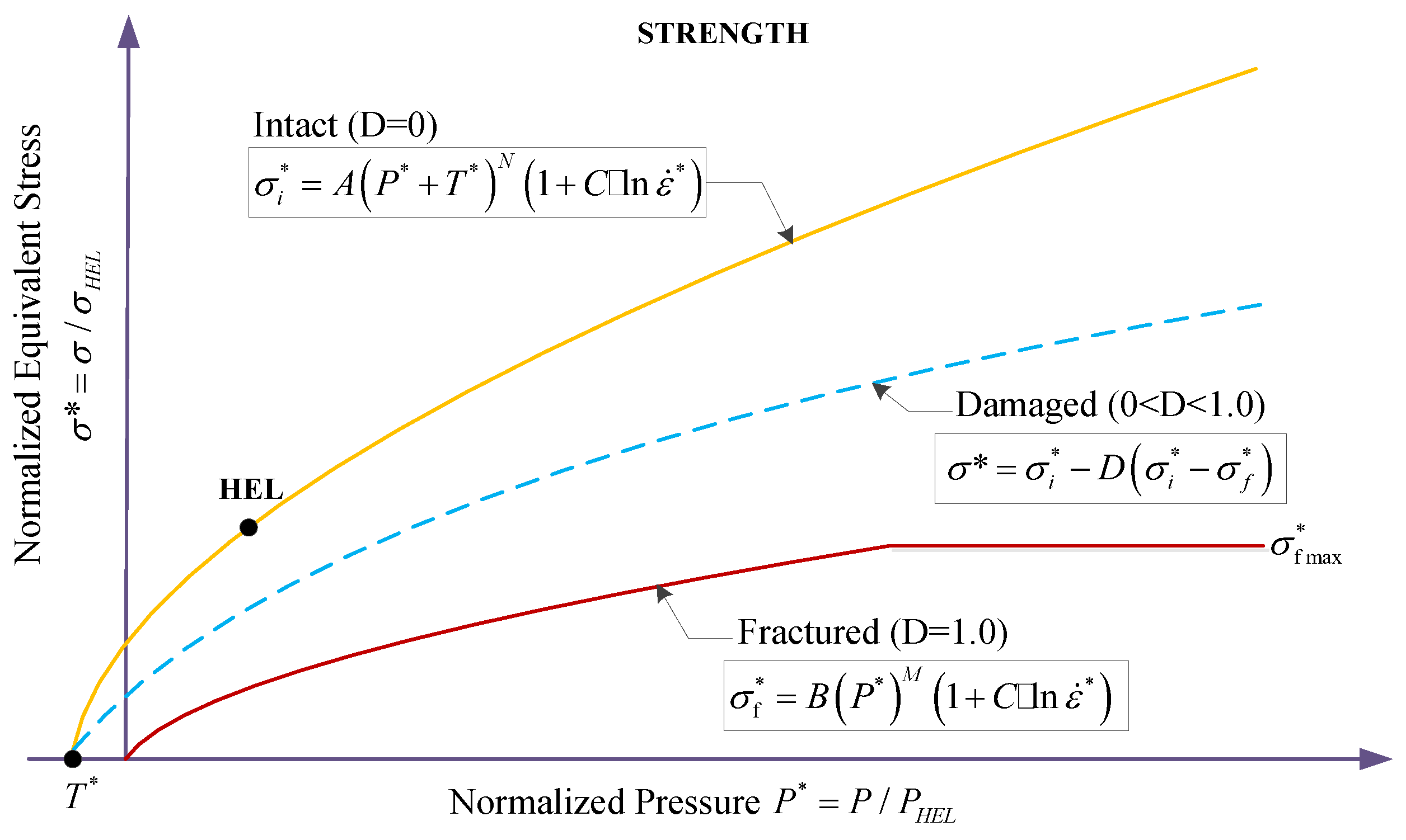
The JH-2 constitutive model was initially utilized to simulate the behavior of brittle materials, especially ceramics. Based on its original concept presented in [2], the JH-2 model adds softening characteristics and contains pressure-dependent strength, damage, and fracture; significant strength after fracture; bulking; and strain rate effects. A general overview of the model is provided in Figure 1 and Figure 2.

2.1. Strength

Figure 1 describes the strength curve of brittle materials from three aspects: the intact state, damaged state, and fractured state. Different states have their own strength equation which presents the relation of normalized equivalent stress versus normalized pressure. The analytic function in damaged state can be considered as the general form for the three states, and its normalized equivalent stress is expressed as

$${\sigma }^{\ast }={\sigma }_i^{\ast }-D\left({\sigma }_i^{\ast }-{\sigma }_f^{\ast }\right)=\sigma /{\sigma }_{HEL}$$

(1)

where ${\sigma }_i^{*}$ is the normalized intact equivalent stress, ${\sigma }_f^{\ast }$ is the normalized fracture stress, $D$ is the damage factor ($0\le D\le 1.0$) and ${\sigma }_{HEL}$ is the equivalent stress at the $HEL$—the Hugoniot elastic limit, an important concept that stands for the net compressive stress (containing both hydrostatic pressure and deviator stress components) at which a one-dimensional shock wave with uniaxial strain exceeds the elastic limit of the material [4]. Herein, $\sigma$ is the actual equivalent stress which is calculated by the formula of von Mises stress [36]

$$\sigma =\sqrt{\frac{1}{2}\left[{\left({\sigma }_x-{\sigma }_y\right)}^2+{\left({\sigma }_x-{\sigma }_z\right)}^2+{\left({\sigma }_y-{\sigma }_z\right)}^2+6\left({\tau }_{xy}^2+{\tau }_{xz}^2+{\tau }_{yz}^2\right)\right]}$$

(2)

or

$$\sigma =\sqrt{\frac{1}{2}\left[{\left({\sigma }_1-{\sigma }_2\right)}^2+{\left({\sigma }_1-{\sigma }_3\right)}^2+{\left({\sigma }_2-{\sigma }_3\right)}^2\right]}$$

(3)

where ${\sigma }_x$, ${\sigma }_y$, and ${\sigma }_z$ are the three normal stresses, ${\tau }_{xy}$, ${\tau }_{xz}$, and ${\tau }_{yz}$ are the three shear stresses, and ${\sigma }_1$, ${\sigma }_2$, and ${\sigma }_3$ are the three principal stresses.

The normalized intact strength is given by

$${\sigma }_i^{\ast }=A{\left(P^{\ast }+T^{\ast }\right)}^N\left(1+C\cdot \ln {\dot{\epsilon }}^{\ast }\right)$$

(4)

The normalized fracture strength is given by

$${\sigma }_f^{\ast }=B{\left(P^{\ast }\right)}^M\left(1+C\cdot \ln {\dot{\epsilon }}^{\ast }\right)\le SFMAX$$

(5)

where $A,B,C,M,N$ are material constants, the normalized pressure is $P^{\ast }=P/P_{HEL}$, where $P$ is the actual hydrostatic pressure, and $P_{HEL}$ is the hydrostatic pressure at the $HEL$. The normalized maximum tensile hydrostatic pressure is $T^{\ast }=T/P_{HEL}$, where $T$ is the maximum tensile hydrostatic pressure the material can withstand. The dimensionless strain rate is ${\dot{\epsilon }}^{\ast }={\dot{\epsilon }/\dot{\epsilon }}_0$, where $\dot{\epsilon }$ is the actual equivalent strain rate and ${\dot{\epsilon }}_0=1.0s^{-1}$ is the reference strain rate. $SFMAX$ is the ultimate value of ${\sigma }_f^{\ast }$ that provides extra flexibility in defining the fracture strength. The actual equivalent strain rate is analogous to the equivalent stress and is expressed as

$$\dot{\epsilon }=\sqrt{\frac{2}{9}\left[{\left({\dot{\epsilon }}_x-{\dot{\epsilon }}_y\right)}^2+{\left({\dot{\epsilon }}_x-{\dot{\epsilon }}_z\right)}^2+{\left({\dot{\epsilon }}_y-{\dot{\epsilon }}_z\right)}^2+\frac{3}{2}\left({\dot{\gamma }}_{xy}^2+{\dot{\gamma }}_{xz}^2+{\dot{\gamma }}_{yz}^2\right)\right]}$$

(6)

where ${\dot{\epsilon }}_x$, ${\dot{\epsilon }}_y$, and ${\dot{\epsilon }}_z$ are the three normal strain rates; and ${\dot{\gamma }}_{xy}$, ${\gamma }_{xz}$, and ${\gamma }_{yz}$ are the three engineering shear strain rates.

In the JH-2 constitutive model, the brittle material begins to soften when damage starts to accumulate (see the damage curve in Figure 1). The softening process can be expressed by Equation (1), which allows for gradual softening of the material under increasing plastic strain, although the softening does not continue when the material is completely damaged ($D=1$).

2.2. Damage

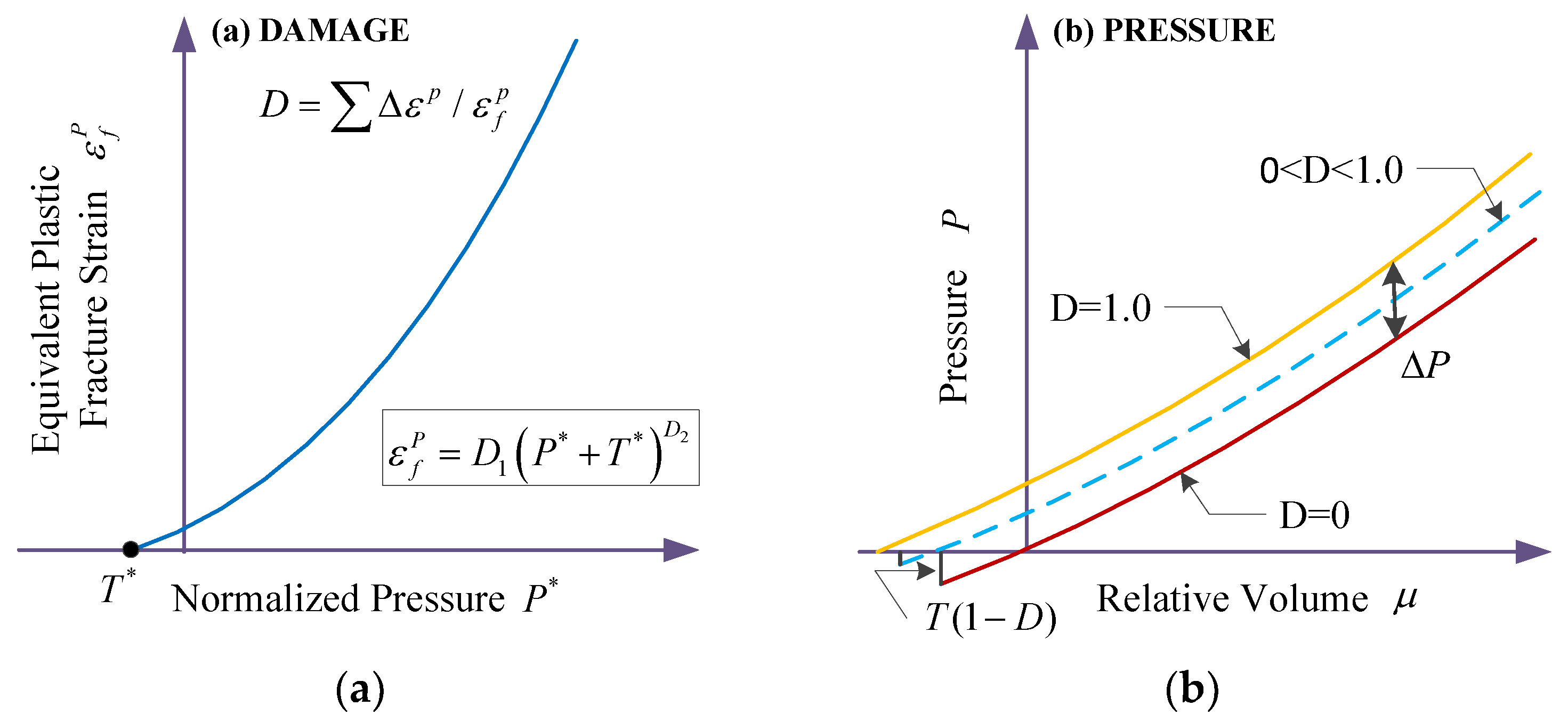
The changed tendency of damage presenting nonlinear increase is shown in Figure 2a. The expression of accumulated damage caused by fracture is

$$D={\displaystyle \sum \Delta {\epsilon }^P/{\epsilon }_f^P}={\displaystyle \sum \Delta {\epsilon }^P/\left[D_1{\left(P^{\ast }+T^{\ast }\right)}^{D_2}\right]}$$

(7)

where $\Delta {\epsilon }^P$ is the plastic strain during a cycle of integration, ${\epsilon }_f^P=f\left(P\right)$ is the plastic strain to fracture under a constant pressure $P$, and $D_1$ and $D_2$ are the damage factors for ${\epsilon }_f^P$.

2.3. Polynomial Equation of State (EOS) of Pressure

In physics, when the plastic deformation or damage of a unit accumulates to a certain threshold, the material undergoes failure and loses strength, in what is called near-fluid-like behavior [4], in which the unit cannot withstand any stress, but the hydrostatic pressures and the deviatoric stress are equal to zero. Herein, the polynomial equation of state (EOS) presents the relationship between hydrostatic pressure, $P$ and volumetric strain, $\mu$ (Figure 2b), which consists of a pure elastic stage and a plastic damage stage. The detailed expressions are given by

$$\{\begin{array}{l}P=K1\cdot \mu +K2\cdot {\mu }^2+K3\cdot {\mu }^3................(D=0)\\ P=K1\cdot \mu +K2\cdot {\mu }^2+K3\cdot {\mu }^3+\Delta P.......(0<D\le 1)\end{array}$$

(8)

where K1, K2, and K3 are constants (K1 is the bulk modulus) and $\mu =\rho /{\rho }_0-1$ for current density $\rho$ and initial density ${\rho }_0$. For tensile pressure ($\mu <0$), Equation (8) is replaced by $P=K1\cdot \mu$. Incremental pressure, $\Delta P$, is added when fracture occurs in the material, which is caused by the bulking energy.

The incremental internal elastic energy decrease is converted to potential internal energy by incrementally increasing $\Delta P$. The shear and deviator stresses decrease due to the decrease of the equivalent plastic flow stress, $\sigma$, as the fracture increases. The elastic internal energy of the shear and deviator stresses is expressed as

$$U={\sigma }^2/6G$$

(9)

where $G$ is the shear modulus of elasticity.

The incremental energy loss is

$$\Delta U=U_{D(t)}-U_{D(t+\Delta t)}$$

(10)

where $U_{D(t)}$ and $U_{D(t+\Delta t)}$ are calculated from Equation (9) using $\Delta U=U_{D(t)}-U_{D(t+\Delta t)}$ for both energies.

The energy loss $\Delta U$ is mainly converted to the fracturing energy $\Delta F$. An approximate equation for this energy conservation is

$$\Delta F=\beta \cdot \Delta U$$

(11)

where $\beta$ is the fraction ($0\le \beta \le 1$) of the elastic energy loss converted to the fracturing energy.

3. Parameter Determination Method for the JH-2 Model

The parameter determination for the JH-2 model is not a straightforward process as some of the constants cannot be determined explicitly [4]. Barre granite is a typical hard and brittle igneous rock [37], which is extensively quarried throughout the Barre granite quarry district in the vicinity of the towns of Websterville and Graniteville, Vermont, USA [29]. The fundamental physical and mechanical parameters of the Barre granite can be obtained from Banadaki and Mohanty [29,30], which includes the average density $\rho =2.66\mathrm{g}/\mathrm{c}{\mathrm{m}}^3$, the longitudinal wave velocity $V_P=4.53\mathrm{km}/\mathrm{s}$, the shear wave velocity $V_S=2.87\mathrm{km}/\mathrm{s}$, the dynamic Poisson’s ratio ${\nu }_d=0.16$, the dynamic Young’s modulus $E_d=50.79\mathrm{GPa}$, the dynamic shear modulus $G_d=21.87\mathrm{GPa}$, and the dynamic bulk modulus $K1=K_d=25.65\mathrm{GPa}$.

3.1. Determination of Parameters Concerned with HEL

In the JH-2 constitutive model, $HEL$ is an important concept throughout the whole computational process. Before determining the parameters of the JH-2 model, it should be noted that the normalized parameters are all derived based on the constants concerned with $HEL$, such as ${\sigma }_{HEL}$ and $P_{HEL}$ introduced above. Therefore, it is the primary task to obtain the values of $HEL$, ${\sigma }_{HEL}$, and $P_{HEL}$. $HEL$ is usually measured from the mechanical response of rock materials determined using flyer plate impact experiments using a light gas gun [38] or explosives [39]. With regard to granitic rock, Kingsbury et al. [40] proposed that the Hugoniot properties of Atlanta granite are similar to those of dolerite, the $HEL$ value of which is around 4–5 GPa through a series of plate impact experiments. Petersen [41] determined a specific average value of $HEL$ of 4.5 GPa for granite, which has been extensively adopted in recent dynamics research [26,29,30]. Therefore,$HEL=4.5\mathrm{GPa}$ is considered as a reliable experimental parameter used in the simulation in this study.

For brittle materials, the relationship between the equivalent stress, ${\sigma }_{HEL}$, and the hydrostatic pressure, $P_{HEL}$, at the $HEL$ [42] is given by

$$P_{HEL}=\frac{V_P^2}{V_S^2}\frac{{\sigma }_{HEL}}{2},$$

then

$$P_{HEL}=1.246{\sigma }_{HEL}$$

(12)

where $V_P$ is the longitudinal wave velocity and $V_S$ is the shear wave velocity.

The expression of $HEL$ is given as follows according to [3]

$$HEL=K1\cdot {\mu }_{HEL}+K2\cdot {\mu }_{HEL}^2+K3\cdot {\mu }_{HEL}^3+\frac{4}{3}G\left(\frac{{\mu }_{HEL}}{1+{\mu }_{HEL}}\right)=P_{HEL}+\Delta P$$

(13)

As can be obtained from Equation (13), $\Delta P=\frac{4}{3}G\left(\frac{{\mu }_{HEL}}{1+{\mu }_{HEL}}\right)$ is the increased potential internal energy converted from the internal elastic energy, which is due to the decreased deviatoric stress. Then $P_{HEL}$ can be expressed as

$$P_{HEL}=HEL-\frac{4}{3}G\left(\frac{{\mu }_{HEL}}{1+{\mu }_{HEL}}\right)$$

(14)

Therefore, the deviatoric strength component is $S_z=-\left(HEL-P_{HEL}\right)$. The sum of the three deviatoric stresses must be zero by the definition $S_x+S_y+S_z=0$, and hence $S_x=S_y=-S_z/2$. Substituting the normal stresses into Equation (2) gives

$${\sigma }_{HEL}=\frac{3}{2}\left(HEL-P_{HEL}\right)$$

(15)

Combining Equation (12) with Equation (15) gives

$$1.246{\sigma }_{HEL}+\frac{2}{3}{\sigma }_{HEL}=HEL$$

(16)

Then ${\sigma }_{HEL}=2.35\mathrm{GPa}$ and $P_{HEL}=2.93\mathrm{GPa}$. Substituting the stress, pressure, and shear modulus into Equation (14) gives ${\mu }_{HEL}=0.0567$, where the shear modulus $G$ has been computed based on the previous wave velocity measurement, which can also be computed from $E$ and $\nu$ through $K1=E/3\left(1-2\nu \right)$ and $G=E/2\left(1+\nu \right)$.

3.2. Determination of EOS Parameters

As shown in Figure 2b and Equation (8), $K2$ and $K3$ should be calculated from the relationship between hydrostatic pressure, $P$, and volumetric strain ($\mu =\rho /{\rho }_0-1$) under dynamic loading with high pressure levels. Therefore, the Hugoniot relation is introduced, which is expressed as the curve of shock wave velocity, $u_S$, and particle velocity, $u_P$, by

$$u_S=S\cdot u_P+C(\mathrm{m}/\mathrm{s})$$

(17)

where $S$ is the fitting slope of the straight line and $C$ is the bulk sound velocity.

The Hugoniot equations for the conservation of mass and momentum [43,44] can be expressed as

Conservation of mass

$${\rho }_0{u}_S=\rho \left(u_S-u_P\right)$$

(18)

Conservation of momentum

$$P=\rho u_P\left(u_S-u_P\right)={\rho }_0{u}_S{u}_P$$

(19)

Combining Equation (17) with the Hugoniot equations for the conservation of mass (Equation (18)) and momentum (Equation (19)) to determine the shock Hugoniot in the $P-\mu$ plane as

$$P=\frac{{\rho }_0{C}^2\mu \left(1+\mu \right)}{{\left(1-\left(S-1\right)\mu \right)}^2}$$

(20)

The bulk sound velocity $C$ is given by

$$C=\sqrt{V_P^2-\frac{4}{3}{V}_S^2}=3.088\mathrm{km}/\mathrm{s}$$

(21)

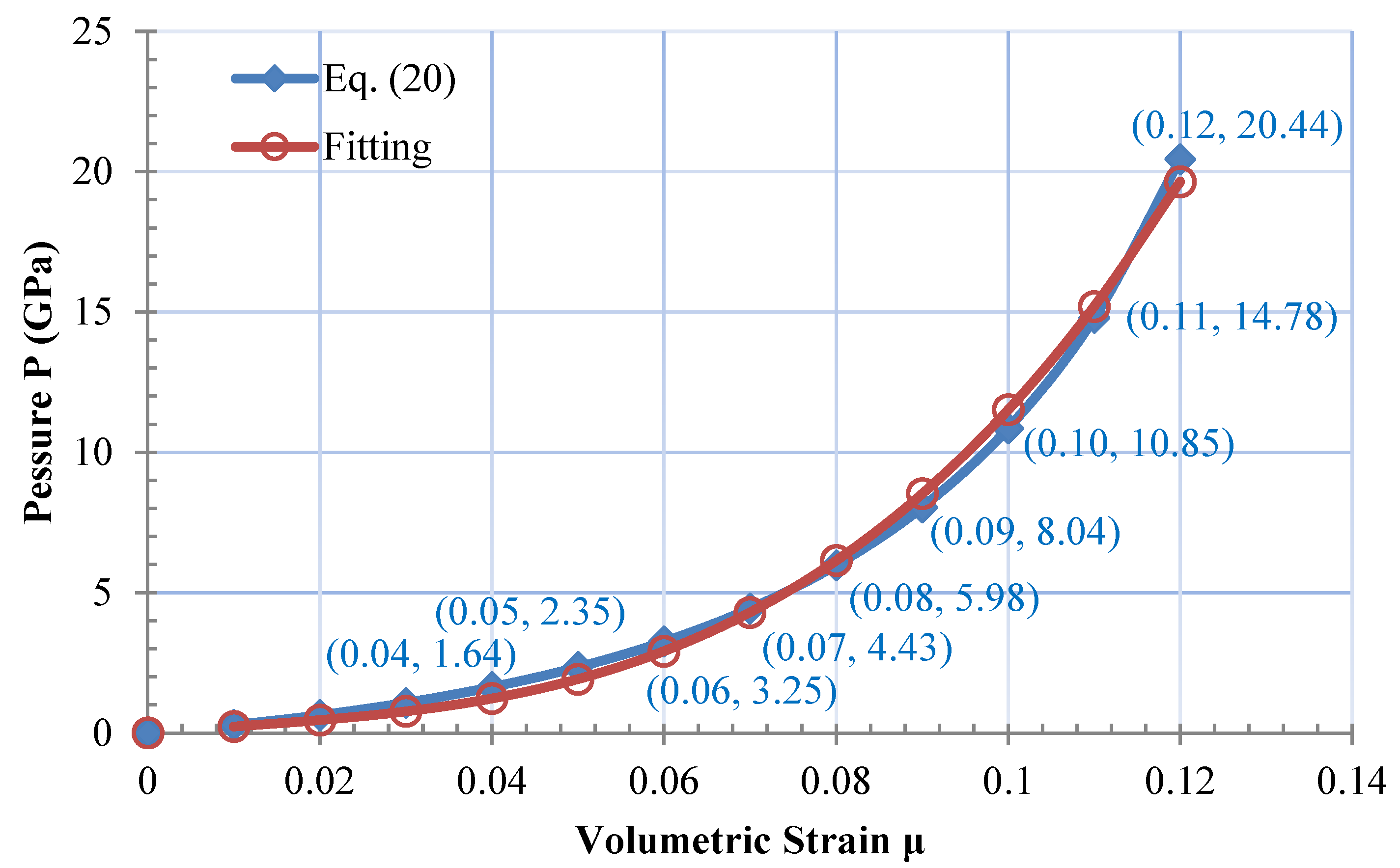
Substituting the previously obtained values of ${\rho }_0$, $C$, $P_{HEL}$, and ${\mu }_{HEL}$ of Barre granite into Equation (20), gives $S=5.93$. Therefore, for Barre granite in this example, Equation (17) can be transformed as

$$u_S^{\prime }=S\cdot u_P^{\prime }+C=5.93u_P^{\prime }+3088(\mathrm{m}/\mathrm{s})$$

(22)

Ideally, it would be better to have shock velocity and particle velocity data from the flyer plate impact tests for Barre granite so that they could be used to fit the linear relationship of Equation (22). However, if there is insufficient data for depicting the relationship, the new extrapolated method above can be chosen in most cases.

Consequently, Equation (20) can be transformed as

$$P=\frac{2.66\times {3.088}^2\times \mu \left(1+\mu \right)}{{\left(1-\left(5.93-1\right)\mu \right)}^2}$$

(23)

By assuming several sets of $P$ and then calculating the corresponding $\mu$ according to Equation (23), the values shown in Figure 3 are used to fit the values of $K2$ and $K3$ in Equation (8) when $D=0$. The obtained fitting values are $K2=-386\mathrm{GPa}$ and $K3=12800\mathrm{GPa}$, and the fitting curve is presented in Figure 3.

Banadaki [29] proposed 2D numerical simulation adjustment to determine the constant values of K2 and K3 (K1 is the bulk modulus previously presented), in which 16 sets of constants in different values of K2 and K3 were assumed for the polynomial EOS. Through the comparison between the results of pressure–distance curves from lab-scale experiments and simulations, the best-fitting values of the constants are obtained as $K2=-4500\mathrm{GPa}$ and $K3=300000\mathrm{GPa}$. However, it is highly demanding to complete these sets of numerical simulations, and the values of K2 and K3 fitted by the results from 2D numerical simulations may have a large deviation, which is not appropriate for use in 3D numerical simulations. Due to different from static problems, the propagation characteristics of stress waves in rock dynamics are complicated and involve some boundary conditions such as the transmission and reflection at boundaries or discontinuities. Therefore, unlike practical experiments, 2D models are prone to generate extra reflection and overlapping of stress waves at artificial boundaries.

3.3. Determination of Strength

The constants concerned with strength are here considered as two portions—the intact strength when the damage factor $D=0$, and the fractured strength when $D=1$.

3.3.1. Determination of Intact Strength

In this section, the constants $A$, $N$, and $C$ will be calculated.

Referring to previous experimental data [29], we set the following parameter values: uniaxial compressive strength (UCS) ${\sigma }_{ci}=167.1\mathrm{MPa}$; triaxial compressive strength (TCS) ${\sigma }_3=5\mathrm{MPa}$, ${\sigma }_1=220.2\mathrm{MPa}$; ${\sigma }_3=10\mathrm{MPa}$, ${\sigma }_1=274.9\mathrm{MPa}$; and equivalent strain rate $\dot{\epsilon }=2.59\times {10}^{-5}$. Reliable estimates for the triaxial compressive strengths of rocks at high confining pressures can be achieved using empirical equations, such as the Drucker–Prager yield criterion [45]. For intact rock pieces that make up the rock mass, the Drucker–Prager yield criterion has the form

$$f\left(I_1,J_2\right)=\alpha I_1+\sqrt{J_2}-k=\alpha \left({\sigma }_1+{\sigma }_2+{\sigma }_3\right)+\sqrt{\frac{1}{6}\left[{\left({\sigma }_1-{\sigma }_2\right)}^2+{\left({\sigma }_2-{\sigma }_3\right)}^2+{\left({\sigma }_1-{\sigma }_3\right)}^2\right]}-k=0$$

(24)

where $I_1$ is the first stress invariant (compression is negative and tension is positive) and $J_2$ is the second invariant of the deviatoric stress. The relationship between the principal stresses at failure for a given rock is defined by two constants, which are $\alpha =2\sin \varphi /\sqrt{3}\left(3-\sin \varphi \right)$ and $k=6c\cdot \cos \varphi /\sqrt{3}\left(3-\sin \varphi \right)$. Due to the shortage of the values of cohesion, $c$, and the internal friction angle, $\varphi$, the values of $\alpha$ and $k$ cannot be directly calculated, but can be obtained by substituting the data of the principal stresses from the previous UCS and TCS experiments into Equation (24). Then Equation (24) can be transformed as

$$f\left(I_1,J_2\right)=0.44\left({\sigma }_1+{\sigma }_2+{\sigma }_3\right)+\sqrt{\frac{1}{6}\left[{\left({\sigma }_1-{\sigma }_2\right)}^2+{\left({\sigma }_2-{\sigma }_3\right)}^2+{\left({\sigma }_1-{\sigma }_3\right)}^2\right]}-22.9=0\left(MPa\right)$$

(25)

In order to depict the relationship between the hydrostatic pressure and equivalent stress of intact granite, a series of data for pressure, $P$, and equivalent stress, ${\sigma }_i$, of intact rock should be obtained. According to the fitting formula in Equation (25), it can be assumed that ${\sigma }_2={\sigma }_3$, the value of which ranges from 0 to 3200 MPa, and can then be substituted into Equation (25) to achieve the value of ${\sigma }_1$. The value of $P$ can be derived from $P=\frac{{\sigma }_1+{\sigma }_2+{\sigma }_3}{3}$ [46]. The value of ${\sigma }_i$ can be calculated using Equation (3). The corresponding data are shown in Figure 4. In these uniaxial and triaxial compression tests, the equivalent strain rate in Equation (6) is $\dot{\epsilon }=2.59\times {10}^{-5}={\dot{\epsilon }}^{\ast }$.

According to previous studies [4,26,47], the maximum tensile hydrostatic pressure $T$ is calculated from the dynamic tensile strength considered as the spall strength by planar impact tests. The dynamic tensile strength of granite can be determined by flyer plate impact tests and is equal to the tensile stress while the incipient tensile cracks begin to happen accompanied by the decrease onset of longitudinal wave. Ai and Ahrens [26] determined the dynamic tensile strength of granite to be 0.13 GPa. Additionally, in plate impact experiments to investigate shock-induced inelasticity in Westerly granite, the mechanical property is weaker than the general granite, and the spall strength is 0.05 GPa [48]. Because it is short of the specific value of the spall strength (dynamic tensile strength), $T_{spall}$, for Barre granite, in this study the intermediate approximate value of (0.05 GPa, 0.13 GPa) was chosen to ensure the magnitude of the spall strength, and a value of $T_{spall}=0.10\mathrm{GPa}$ was assumed. Then, the hydrostatic pressure and equivalent stress at failure can be obtained from Equations (26) and (27) under dynamic uniaxial strain condition [4,28]

$$P=\frac{T_{spall}}{3}\left(\frac{1+\nu }{1-\nu }\right)$$

(26)

$${\sigma }_i=T_{spall}\left(\frac{1-2\nu }{1-\nu }\right)$$

(27)

Substituting $T_{spall}=0.1\mathrm{GPa}$ and $\nu =0.16$ into the equations above gives $P=0.046\mathrm{GPa}$ and ${\sigma }_i=0.081\mathrm{GPa}$. Extrapolating the ${\sigma }_i$ versus $P$ relationship down to ${\sigma }_i=0$ gives the maximum tensile hydrostatic pressure $T=-P_{{\sigma }_i=0}=0.057\mathrm{GPa}$. The normalized tensile strength in Equation (4) is $T^{\ast }=T/P_{HEL}=0.0194$.

The strain rate constant, $C$, which stands for the measure of the strain rate effect, influences both the intact and fractured material strengths. This strain rate constant is calculated based on experimental data at different strain rates. It has been reported that the increase in strength is mainly due to the increased pressure effect [4,20,49]. However, the strain rate effect is also one component of the main factors, especially in the process of high strain rate. To separate the part caused by stain rate effect from the equivalent stress, a technique was used to remove the pressure effect and obtain the strain rate constant $C$. As is shown in Figure 5, the upper line was fitted from the data of SHPB dynamic compressive strength tests under the average strain rate ${\dot{\epsilon }}_2=100$ [50], while the lower line is the line connecting the points of the maximum tension data and the quasi-static triaxial compression data at a constant pressure $P=0.3\mathrm{GPa}$ determined by the standard from [13] under the average strain rate ${\dot{\epsilon }}_1=2.59\times {10}^{-5}$. The fitting functions for the two lines are obtained in Figure 5, and the strain rate constant, $C$, can be calculated from the division between ${\sigma }_{i-1}$ and ${\sigma }_{i-2}$ under different strain rates by combining Equation (4)

$$\begin{array}{cc}\hfill \frac{{\sigma }_{i-1}}{{\sigma }_{i-2}}& =\frac{A\left(P^{*}+T^{*}\right)\left(1+C\ln {\dot{\epsilon }}_2\right)}{A\left(P^{*}+T^{*}\right)\left(1+C\ln {\dot{\epsilon }}_1\right)}=\frac{1+C\ln 100}{1+C\ln \left(2.59\times {10}^{-5}\right)}\hfill \\ & =\frac{\underset{P_1\to +\infty }{\lim }\left(1.895P_1+95.337\right)}{\underset{P_2\to +\infty }{\lim }\left(1.7515P_2+99.835\right)}=1.082\hfill \end{array}$$

(28)

The strain rate constant can be solved from Equation (28) as $C=0.0051$.

When the damage factor $D=0$, the previous triaxial compression data in Figure 4 is chosen to fit the constants $A$ and $N$ in Equation (4), and then the values $A=1.248$ and $N=0.676$ are obtained.

3.3.2. Determination of Fractured Strength

The method with the intact strength above, for fractured state ($D=1$), if the relationship between the pressure and equivalent stress could be worked out, it would be simple to obtain the parameters $B$ and $M$.

The fractured strength data in Figure 6, which is obtained from the data of Martin [51], is derived from laboratory triaxial compression experiments on cylindrical rock samples with radial confining pressures. The fractured state is from crack initiation, initiation of sliding to peak strength. In Figure 6, the lower line in blue includes a maximum normalized facture strength of ${\sigma }_{f\max }^{\ast }=0.16$. Therefore, it can be assumed that the laboratory triaxial compression test is carried out at complete fracture state with damage factor $D=1$. Consequently, the values $B=0.68$ and $M=0.83$ can be obtained through the fitting of the fracture data above based on the fundamental equation of Equation (5).

3.4. Determination of Damage

Damage (D) describes the transition from intact to fractured strength [26] and begins to accumulate when brittle material starts to flow plastically and then is softened due to a change from large to smaller particle size. A value of $D=1$ is defined when the material is completely damaged. According to the definition of constants $D1$ and $D2$ in Equation (7), if the tendency change of the pressure dependent fracture strain ${\epsilon }_f^P$ following the pressure $P^{\ast }$ can be determined by tests, it would be easy to achieve the constants $D1$ and $D2$ by fitting. Goldsmith et al. [37] performed both tension and compression tests on Barre granite during quasi-static procedures as well as split Hopkinson bar techniques, in which the rock was subjected to a straining deformation at a constant strain rate. The increase of fracture strain presents nonlinear behavior following the increase of constant pressure, as shown in Figure 7 from Goldsmith’s data. Fitting the data based on Equation (7) gives the constants $D1=0.008$ and $D2=0.435$. If there are not enough data, or it is difficult to measure plastic strain directly, especially for some low ductility materials, in order to depict the relationship between fracture strain and pressure, numerical adjustment is another valid method to obtain the two constants $D1$ and $D2$, to which the computational results can be compared with ballistic experiments that produce dwell, interface defeat and penetration. The detailed method of numerical adjustment is described in [26,29,47]. According to the empirical data, the suggested range of values are $D1\in \left[0.001,0.009\right]$ and $D2\in \left[0.4,2.0\right]$.

All the obtained parameters of Barre granite are listed in

Table 1. Parameters of Barre granite and sandstone

Constants	Barre Granite	Sandstone	Constants	Barre Granite	Sandstone
Density ${\rho }_0$ ($\mathrm{g}/{\mathrm{cm}}^3$)	2.66	2.60	Hugoniot elastic limit HEL ($\mathrm{GPa}$)	4.5	4.5
Shear modulus $G$ ($\mathrm{GPa}$)	21.9	17.8	HEL pressure $P_{HEL}$ ($\mathrm{GPa}$)	2.93	2.6
Intact strength coefficient $A$	1.248	1.01	Bulk factor $\beta$	1.0	1.0
Fractured strength coefficient $B$	0.68	0.68	Damage coefficient $D_1$	0.008	0.005
Strain rate coefficient $C$	0.0051	0.005	Damage coefficient $D_2$	0.435	0.7
Fractured strength exponent $M$	0.83	0.83	Bulk modulus $K1$ ($\mathrm{GPa}$)	25.7	19.5
Intact strength exponent $N$	0.676	0.83	Second pressure coefficient $K2$ ($\mathrm{GPa}$)	−386	−23
Maximum tensile strength $T$ ($\mathrm{GPa}$)	57	45	Third pressure coefficient $K3$ ($\mathrm{GPa}$)	12,800	2980
Maximum normalized fractured strength ${\sigma }_{F\max }^{*}$				0.16	0.18

. In order to verify the validity of the parameters computed and extrapolated above for the JH-2 constitutive model, some comparison works were performed as follows. These obtained parameters are adopted in 3D numerical simulations using arbitrary Lagrangian–Eulerian (ALE)/JH-2 method based on the prototype laboratory rock blasting experiments. Both the crack patterns and measured pressures are in agreement with the results from the lab-scale experiments. The attenuation curves of the pressure and particle peak velocity (PPV) along the radial direction were determined, and the summarized theoretical formulae are deemed to be reasonable through comparison with previous theoretical formulae. Additionally, comparisons of blasting tests separately carried out by the DEM-SPH hybrid method [52] and ALE/JH-2 method demonstrate similar crack patterns formed both in intact rock disks and jointed rock disks. This demonstrates that the computational and extrapolated parameters are reasonable for the JH-2 constitutive model of rock materials. A more detailed description of the process and results of the numerical simulations mentioned above has been elaborated elsewhere [53].

4. Application in Tunnel Smooth Blasting

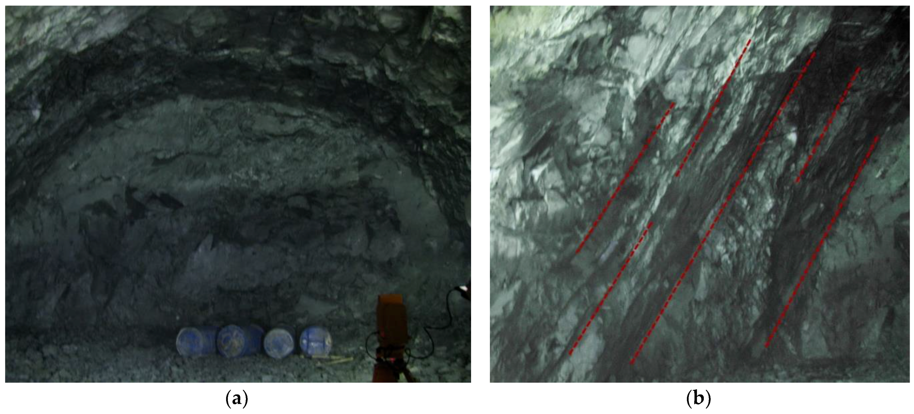
If the JH-2 damage constitutive model could be employed in the constructions of practical engineering, it would be of great help in terms of quality control and prediction in advance, which could improve safety during the constructions and reduce cost. In the case of tunnel excavation, for example, accurate prediction can help decrease the overbreak/underbreak and the vibration on the surrounding rock mass induced by blasting so as to the damage of the surrounding rock mass and improve the entire stability. In this study, the Zigaojian Tunnel of the Hangzhou–Huangshan high-speed railway, China, was chosen as a case study to simulate the process of smooth blasting excavation based on the JH-2 constitutive model. The bedded rock mass structure is distributed in a long (several miles) segment, which consists of large and long bedded discontinuities, occurring on average every 1.5 m and parallel with each other (see Figure 8). Smooth blasting method is used in this tunnel, which means that the explosives detonate from the inner cut boreholes to the external peripheral boreholes in sequence and finally form a smooth tunnel profile.

In general, the determination of rock mass classification is significant before designing for tunnels. Such classification includes information on the strength of the intact rock material, the spacing, the number and surface properties of structural discontinuities, as well as allowances for the influence of subsurface groundwater, in situ stresses, and the orientation and inclination of dominant discontinuities [54]. Many rock mass classification systems have been proposed to date, of which Terzaghi classification, Lauffer classification, Deere’s rock quality designation (RQD), and Wickham’s rock structure rating (RSR) are considered as the earlier main classification methods. However, the influences caused by the properties of discontinuities or intact rock material were disregarded in some of the previous classifications of rock masses [55]. Bieniawski [56,57] developed a modified geomechanical rock mass rating (RMR) classification system, which is used for the design and construction of excavations in rock, such as tunnels, mines, slopes, and foundations. Barton et al. [58,59] proposed a quantitative classification of rock mass (Q-system) as a rock tunneling quality index, on which design and support recommendations for underground excavations are based. The two systems mentioned above are the most influential classification systems proposed to date. Additionally, some other classifications have been developed which are widely adopted in different fields, such as the New Austrian tunneling method (NATM), size-strength classification, International Society for Rock Mechanics (ISRM) classification, geological strength index (GSI), and the BQ method used in China [54,55,56,57,58,59,60]. According to the rock mass classification systems of the corresponding standard [60,61], the bedded structure tunnel investigated in the present study has a surrounding rock ranking of III.

4.1. 3D Numerical Modelling of Smooth Blasting Tunnel

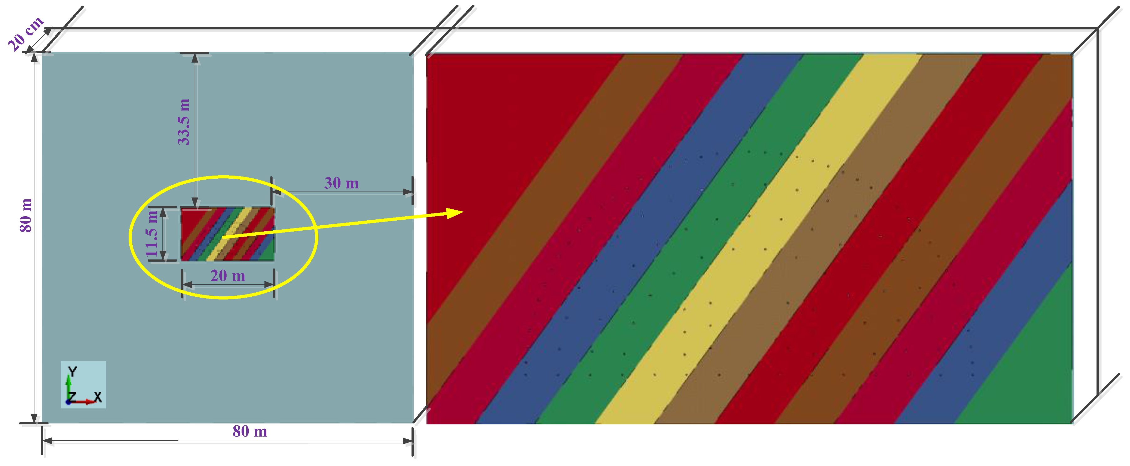
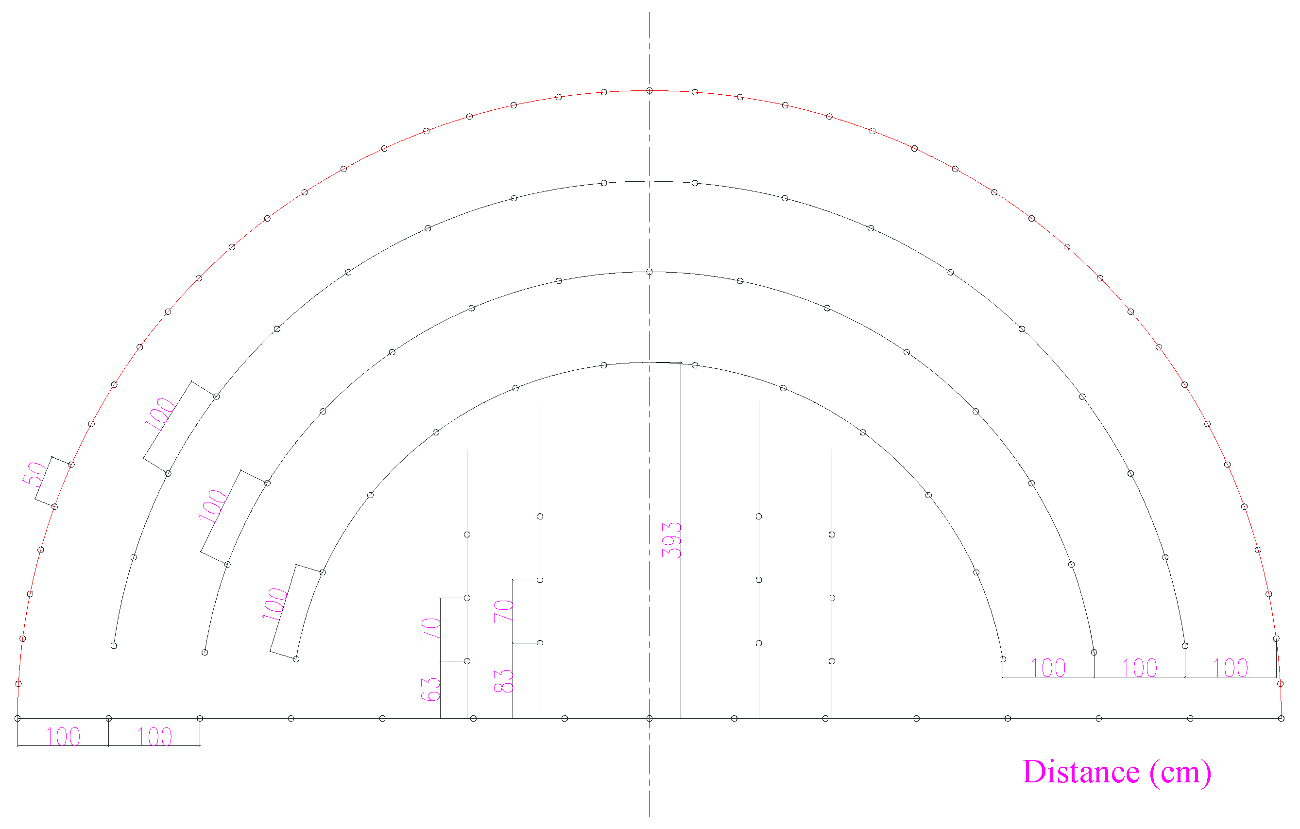
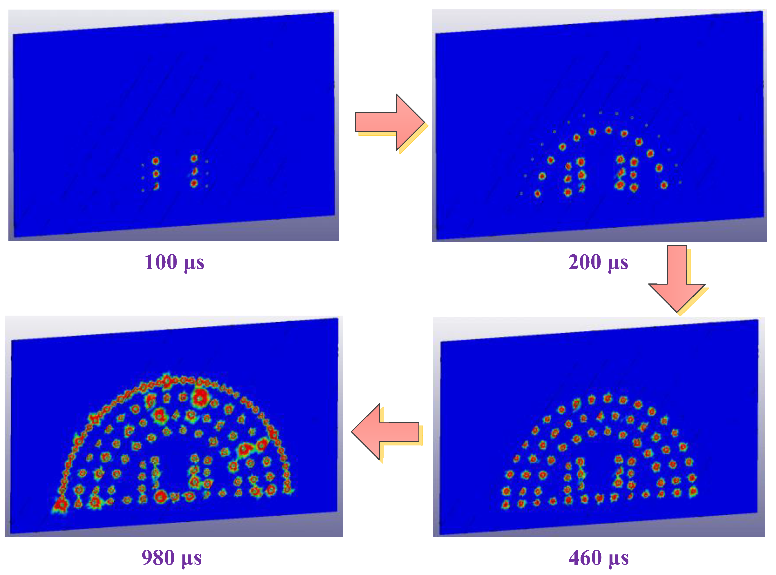
The 3D numerical model of the tunnel with bedded joints is shown in Figure 9. The average dip direction and dip of the parallel joints is $-{22}^{\circ }\angle {56}^{\circ }$ relative to the direction of the tunnel, and the spacing between the two adjacent joints is 1.5 m within the rock mass of sandstone. In order to maintain the progressing level of the running in hydrocode, the thickness of the entire model, as well as the length of all the boreholes, is set as 20 cm. The tunnel design contour is semicircular in shape, with a radius of 6.93 m. A total of 150 boreholes are arranged in the tunnel face with diameters of 4 cm; the detailed layout for the boreholes is shown in Figure 10. The emulsion explosive has a diameter of 3.2 cm and a length of 20 cm. It was assumed that all the explosives are charged in the center of the boreholes, and decoupling charge means is adopted in this practical blasting. The spacing between the explosive and borehole is filled with air. The ALE/JH-2 programmed algorithm [53] is adopted to simulate the rock breaking process induced by blasting. The rock is modeled using Lagrangian material while the air and explosives are modeled by ALE. The finite element meshes used for discretization of the rock are tetrahedron shaped in 3D space; the average element size is 3.0 cm around the boreholes and gradually increases outwards. The rear boundary of the whole model is constrained in XOY plane and defined as the non-reflection boundary, which means that all the waves can penetrate the boundary without reflection just as in transmission in continuous media. The detailed parameters of the sandstone are listed in Table 1 and are obtained using the computational and extrapolated methods proposed before. For the properties of the joints, automatic surface-to-surface contact is adopted in the hydrocode, and it is assumed that the joint surface has no cohesive strength, the dynamic friction coefficient is 0.30 and the tensile strength is zero [62]. The parameters of the emulsion explosives are listed in

Table 2. Parameters of emulsion explosives

Explosive	$\mathit{\rho }$$/\mathbf{g}\cdot {\mathbf{cm}}^{-3}$	$\mathit{D}$$/\mathbf{cm}\cdot \mathsf{\mu }{\mathbf{s}}^{-1}$	${\mathit{p}}_{\mathit{c}\mathit{j}}/105\mathbf{MPa}$	A/105 MPa	B/105 MPa	R1	R2	ω	${\mathit{E}}_0$$/{10}^2\mathbf{GJ}\cdot {\mathbf{m}}^{-3}$	V0
E. 1	1.60	0.550	0.096	5.576	0.0535	6.1	1.07	0.24	0.041	1.0
E. 2	1.26	0.527	0.081	5.576	0.0535	6.1	1.07	0.24	0.041	1.0

, where ‘E. 1’ and ‘E. 2’ represent the explosives charged in the inner cut boreholes and the periphery boreholes, respectively, and the initial detonation positions are at the back of the boreholes. The threshold value of the effective strain is set as 1.0. Once this value is exceeded, the local element would be deleted in order to prevent excessive large deformation during the running of the numerical model. The detailed blasting process is shown in Figure 11; different colors represent different degrees of rock, which will be elaborated later in this study.

4.2. Relation between Crucial Damage Zone and Practical Overbreak

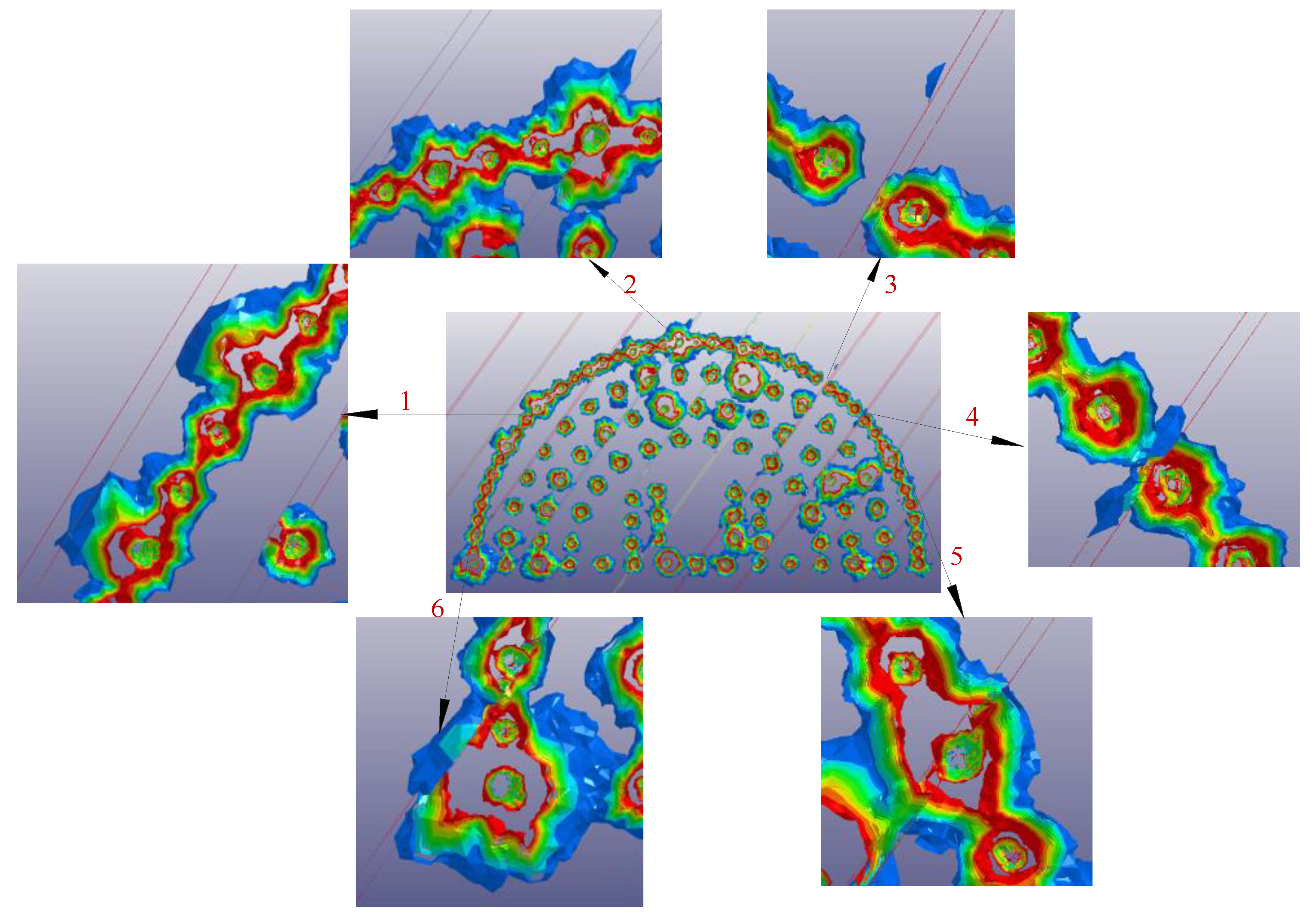
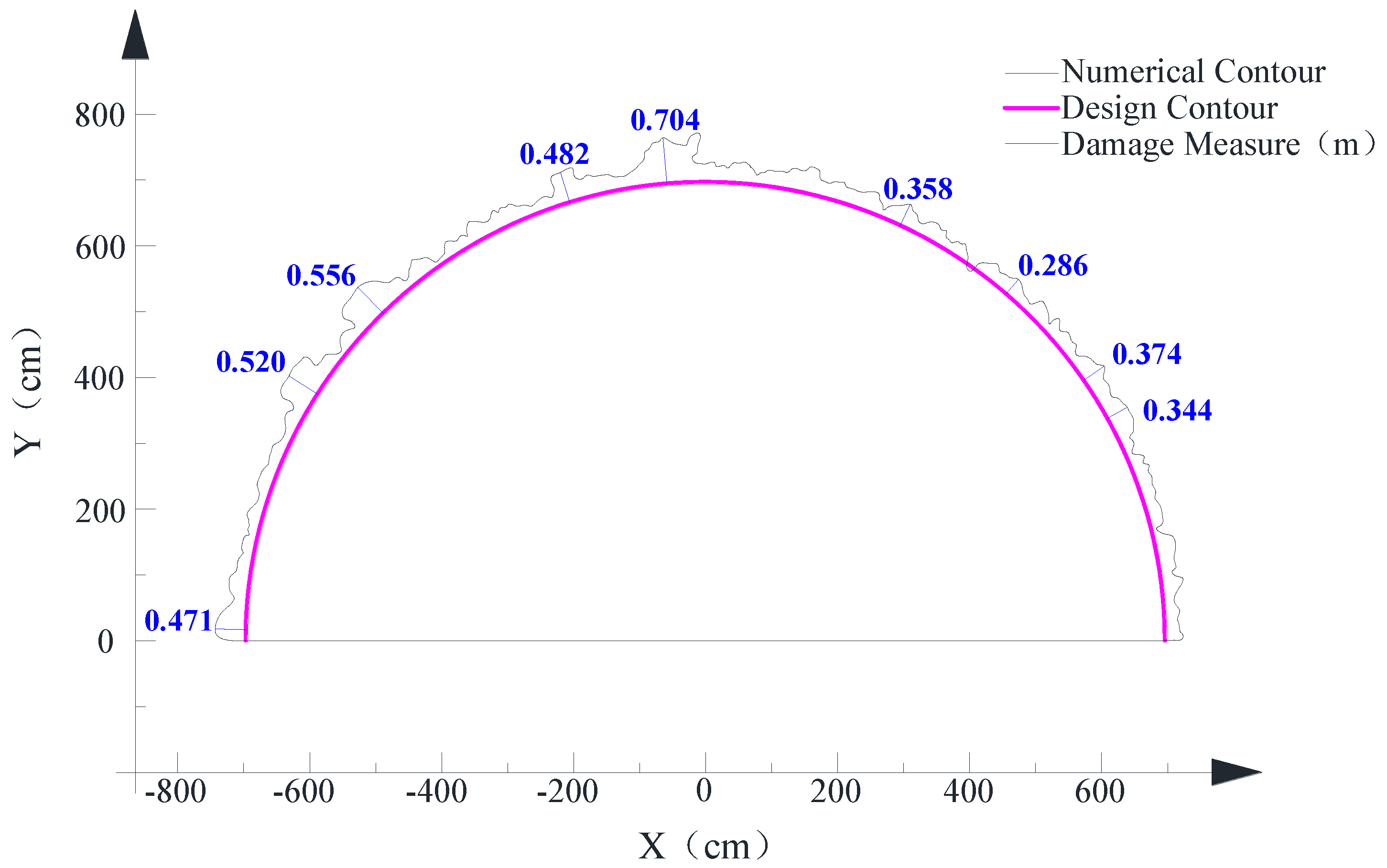
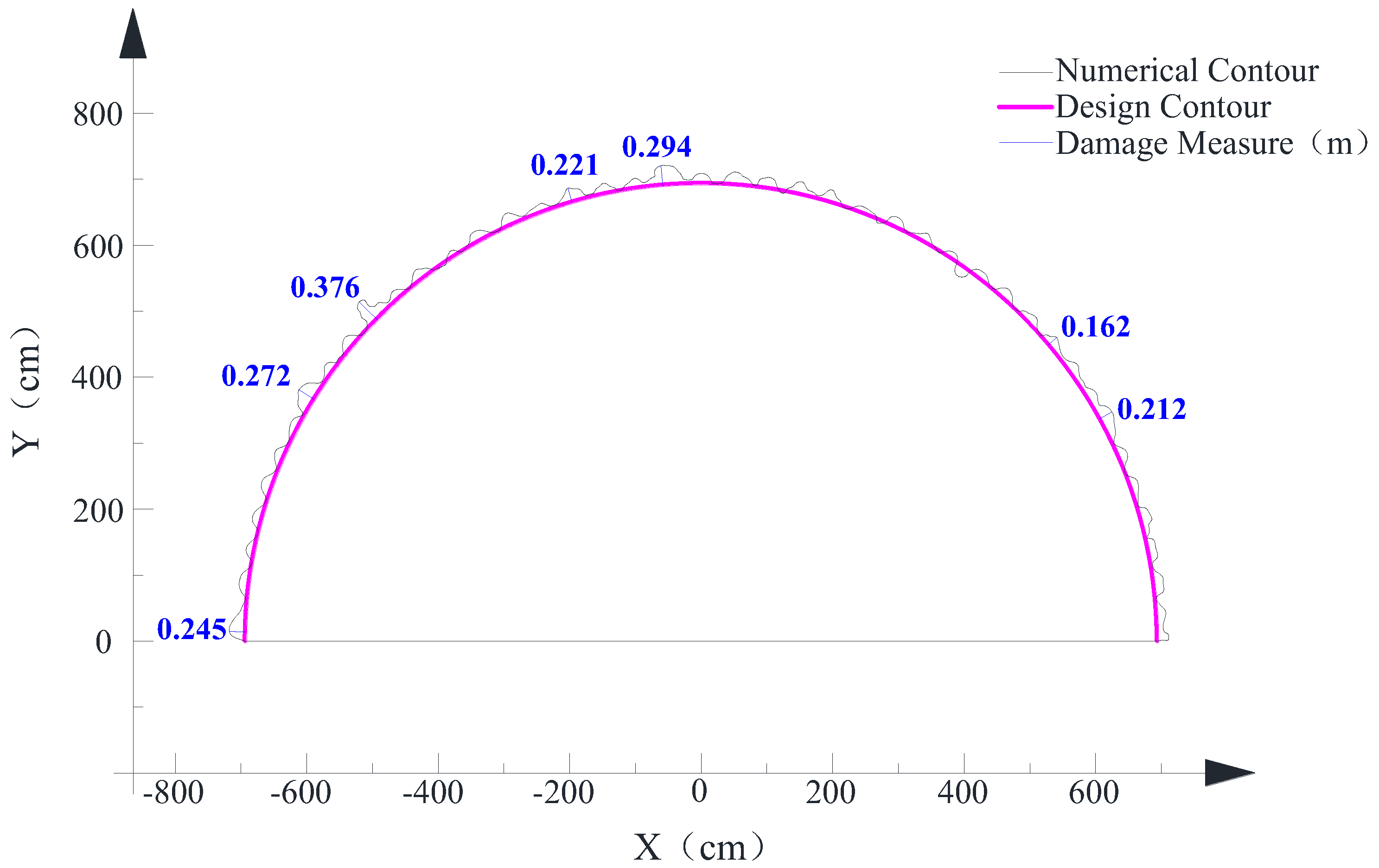
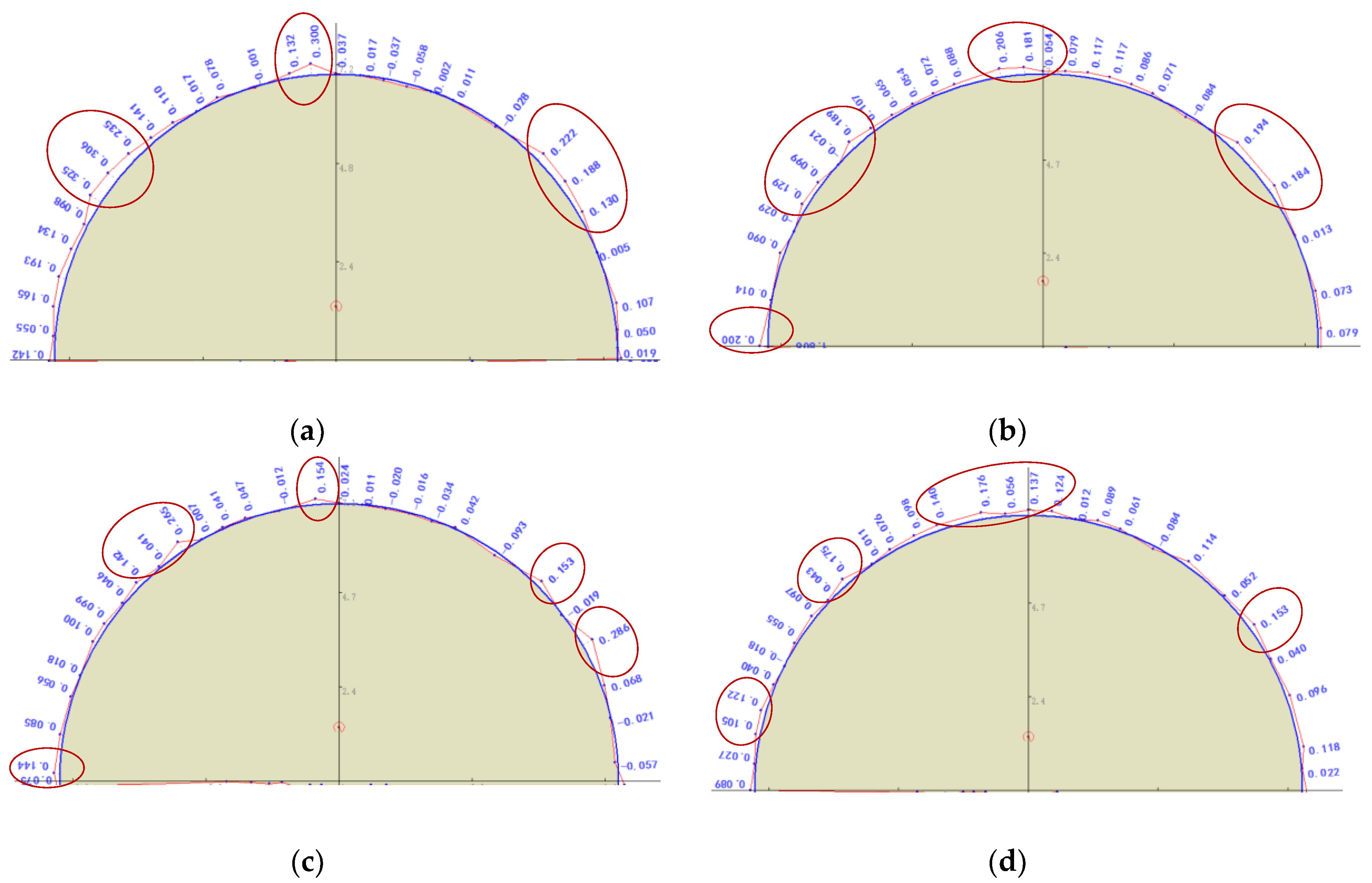
Figure 12 shows the perspective view of the final damage accumulation after the complete blasting of all the explosives. The crucial damage degree and scope distribution in the surrounding rock mass is represented by different colors—the damage degree decreases in a gradient from red to green to blue in damage contours and the damage scope tends to be degraded from the detonating position to the external free surface based on the observation of 3D damage contour. In the interest of quantifying the degree of damage for the numerical damage contour, the outermost damage contours in blue and in red are traced and presented as curves along the design contour (see Figure 13 and Figure 14). The larger damage positions are recognized by measuring the spacing between the numerical damage contour and the design contour. Additionally, four section profiles of this blast round were also measured using a tunnel profilometer at the Zigaojian Tunnel site (see Figure 15), where the overbreak and underbreak are labeled by the data along the design contour and the main overbreak positions are circled by red ellipses. By comparing the main overbreak positions measured from the site in Figure 15 with the main damage positions from the numerical study in Figure 13, the main distributed positions for overbreak and damage are observed to match well with each other. However, the main overbreak values are smaller than the values of damage zone estimated by the damage contour in blue, while being approximately consistent with the values of damage zone estimated by the damage contour in red (See Figure 13, Figure 14 and Figure 15). Therefore, the red damage contour can be used to estimate the overbreak/underbreak values for the excavation of smooth blasting tunnel through the numerical study. On the other hand, it also reflects the validity of the numerical study according to the analysis of the relation between the crucial damage zone and the practical overbreak above.

4.3. Damage Influenced by Bedded Joints

In the quality system for evaluating smooth blasting tunnels, it is necessary to focus on studying the overbreak/underbreak and damage of the surrounding rock mass [63,64,65,66]—especially for the tunnel investigated in the present study, which has a bedded rock mass structure—while the influence induced by joints should be also considered. Six representative positions of the 3D damage contour are chosen to be amplified and labeled from ‘1’ to ‘6’ as shown in Figure 12. It can be classified into four situations to discuss: Situation 1 (e.g., Location 1) shows that the joint nearly parallel to the part of the peripheral holes enhanced the overbreak at individual boreholes and the degree of damage along the joint, which indicates that strong reflection of stress wave occurred at the joint and the damage increased due to the overlap of the stress waves. In Situation 2 (e.g., Locations 2 and 5) the boreholes are located exactly on the joint, which seems to more easily cause overbreak and large-scale damage due to the weak mechanical properties of joints that facilitate the generation of cracks along the joints. In Situation 3 (e.g., Location 3), the joint located between the two boreholes impeded the generation of penetrating cracks which could help form a smooth profile for the tunnel. Therefore, the underbreak formed near to the joint. Moreover, damage was caused at a further position along the joint, which may be the result of the enhanced effect of stress waves close to the joint. Situation 4 (e.g., Locations 4 and 6) is similar to Situation 3, however the joint is closer to one of the boreholes, which caused more damage along the joint and affected the thorough connection between the boreholes (short of red damage contour). In summary, the joint position could change the direction of damage expansion and distinctly influence the degree of damage in the surrounding rock mass. Referring to the four situations discussed above, measures such as increasing or decreasing charge quantity could be adopted to decrease the overbreak and damage for the surrounding rock mass according to the different relative positions between boreholes and joints.

4.4. Damage in Large Scope Estimated by PPV

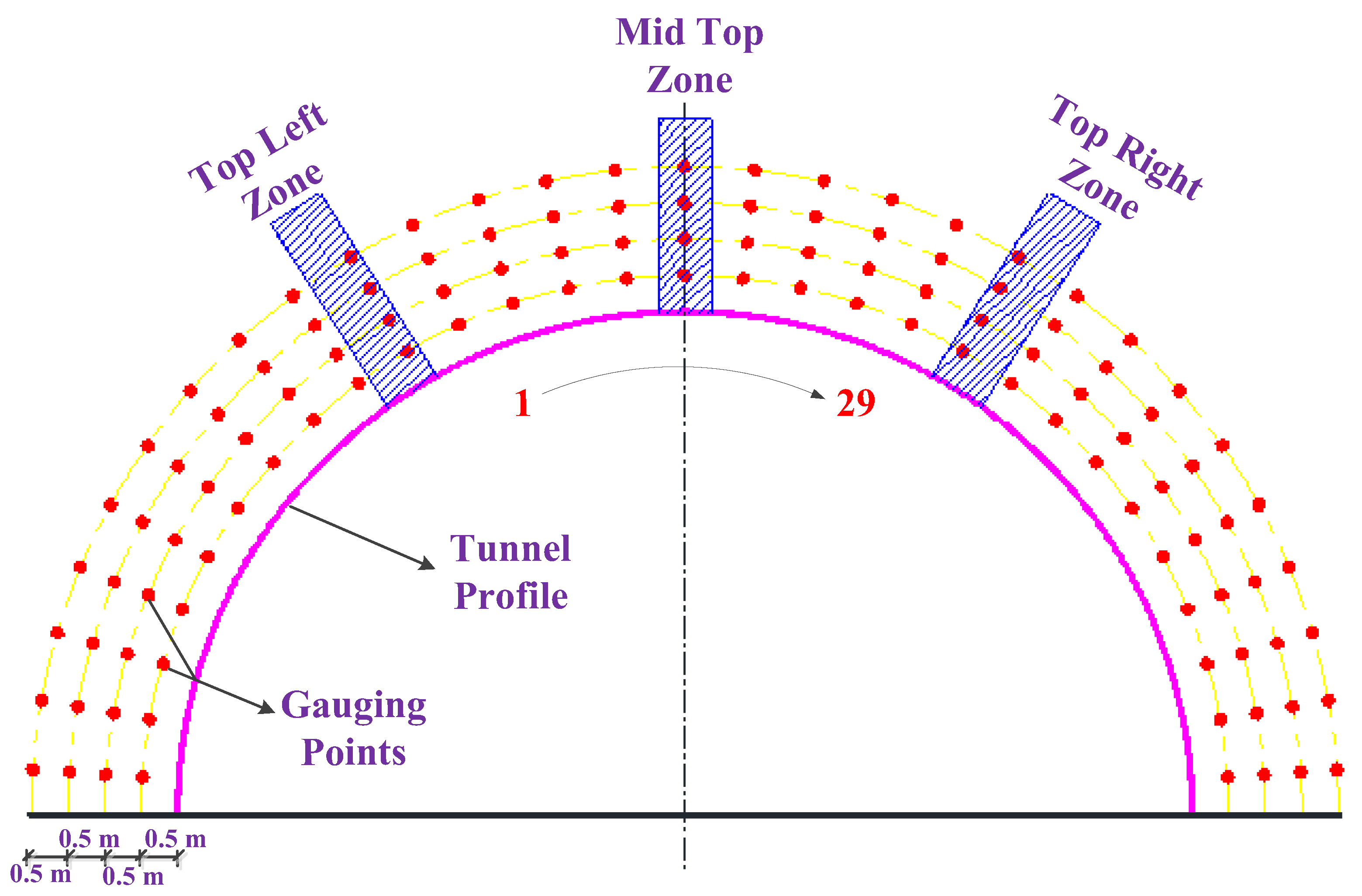
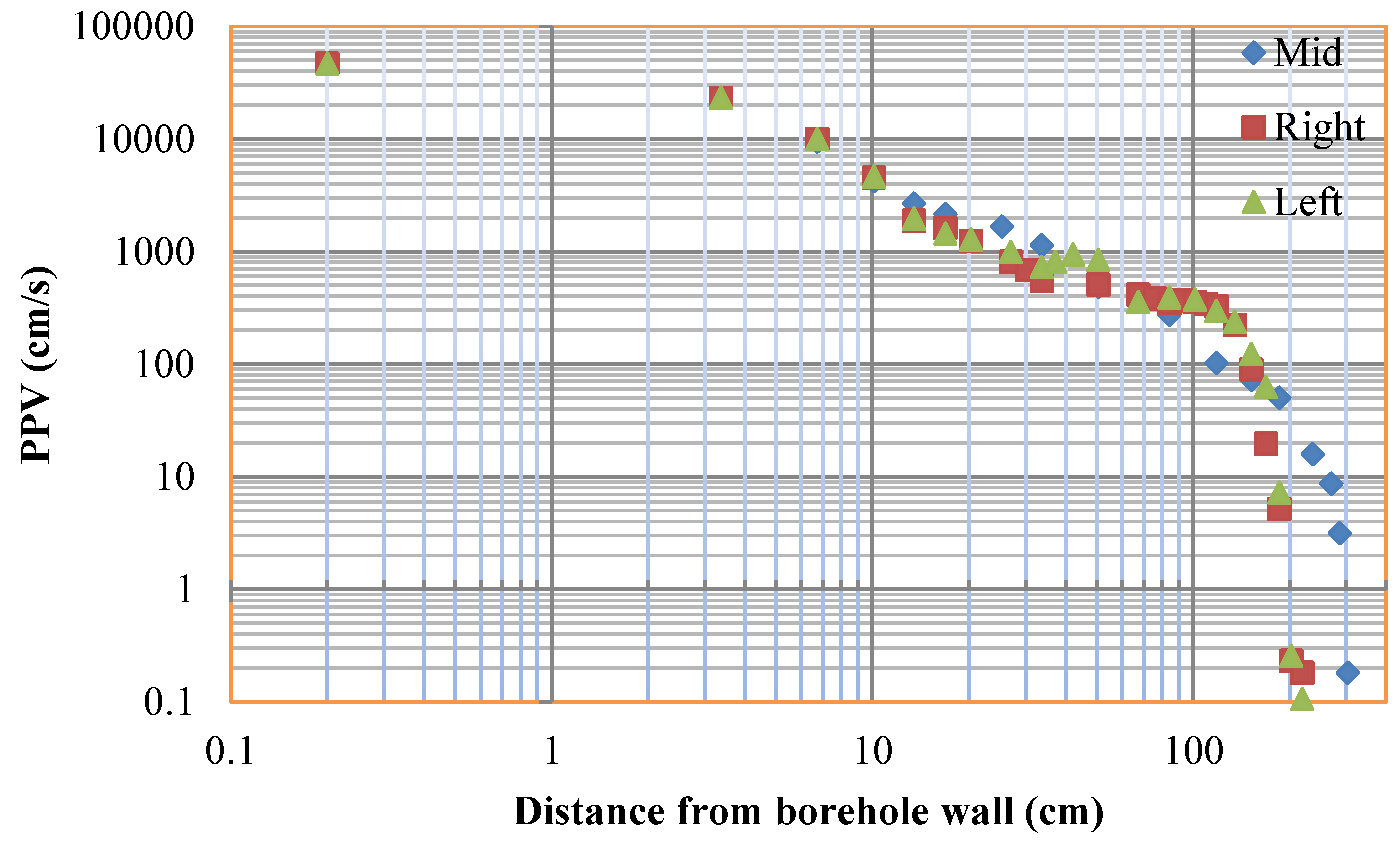
In terms of the extent of large-scale damage, various estimation methods are currently available, e.g., the PPV method [67], the criterion of tensile and compressive shear failures [68], the method of release ratios of displacement [69], and damage criterion using Mazars’ model [70]. The PPV method is the most widely used in practical on-site measurement. However, it is usually firstly measured in the far-field (more than 10 m away from the explosion source), and then the PPV in the near-field can be inferred using empirical formulae, which is difficult to estimate accurately. In this study, PPV is measured numerically, and can be more directly obtained in the near-field around the boreholes. It is known that the instability of the tunnel mainly depends on the degree of damage degree to the tunnel vault. Therefore, it is necessary to explore the attenuation law of the PPV in the vault area. As is shown in Figure 16, three zones are chosen to measure the PPV outwards from the borehole walls. The measured PPV values of the corresponding zones can be clearly recognized from the attenuation curves named ‘Left’, ‘Mid’, and ‘Right’ in Figure 17, in which the top left zone has a similar attenuation tendency to the top right zone and attenuated faster than the middle top zone. According to the PPV damage criterion for bedded rock [71] and the PPV damage criterion for unlined rock tunnels [72], the lowest damage extent is incipient damage whose threshold is about 70 cm/s for hard rock. Therefore, the damage scopes of the three positions above can be estimated from Figure 17, in which the damage scope of the middle top is 151.7 cm, the top left is 160.0 cm and the top right is 155.2 cm.

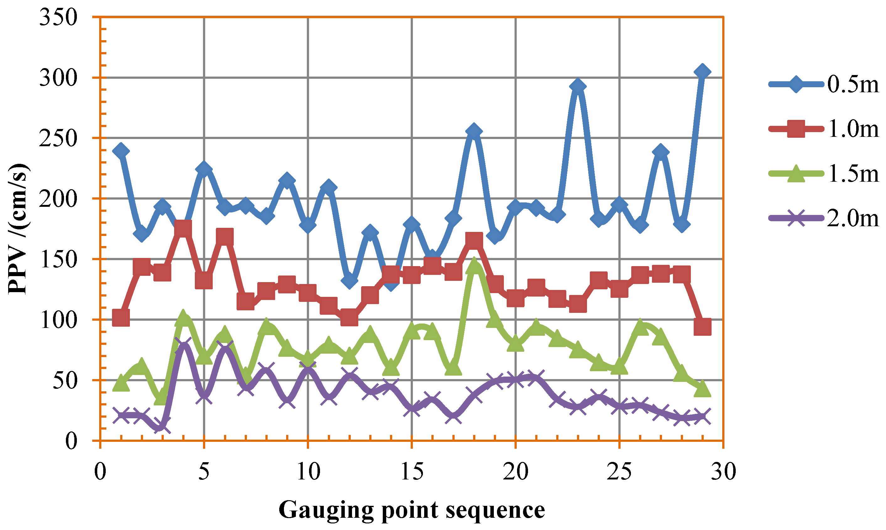
Through a comprehensive study of the PPV values of the whole surrounding rock mass, four groups of gauging points in the surrounding rock mass are measured, which are 0.5, 1.0, 1.5, and 2.0 m away from the design contour of the tunnel. Each group has 29 gauging points uniformly distributed around the design contour (see Figure 16). The PPV curves for different distances are presented in Figure 18. It can be seen that the PPVs with values around 0.5 m have a larger diversity during the 29 gauging points, which is probably caused by the effect of the joints close to the boreholes. In light of the changes of the PPV curves in Figure 18, the PPV values of the four different distances can be sorted into four concentrated ranges, which are shown in

Table 3. Estimation of damage degree by PPV for the bedded tunnel

Distance (m)	PPV Concentrated Range (cm/s)	Average PPV (cm/s)	Damage Degree
0.5 m	150–250	196.3	Serious damage
1.0 m	100–150	130.2	Medium/serious damage
1.5 m	50–100	76.8	Slight/medium damage
2.0 m	30–50	38.1	Basically no damage

, and the damage degrees are estimated according to the PPV damage criteria [71,72].

5. Conclusions

In this study, a determination method for the parameters of the JH-2 constitutive model is conducted in detail using Barre granite rock, in which a new extrapolated method for Hugoniot concerned parameters is proposed as well as the parameters determination methods of strength, EOS, and damage based on data from previous quasi-static and dynamic tests, which further improved the availability of the parameters. In the situation where complicated dynamic experimental data is lacking for the JH-2 constitutive model, the proposed technical route for determining the parameters is a feasible choice.

The JH-2 damage constitutive model is tentatively adopted to simulate the blasting process in the Zigaojian smooth blasting tunnel, which has a bedded rock mass structure, and 3D damage contours are successfully obtained from the numerical simulation. The results show that the overbreak/underbreak induced by rock blasting and joints/discontinuities is well estimated through comparing the damage contours with the tunnel profiles measured from the tunnel site. Furthermore, a series of PPV values are measured by the numerical study, and the scale of near-field damage and degree of damage around the surrounding rock mass are both summarized. All the results mentioned above could provide certain theoretical evidence for optimizing the design of smooth blasting tunnels in practice, such as adjusting the positions of boreholes or regulating the charge quantity in boreholes. However, the precondition of the above is that the characteristics of rock materials should be well mastered as much as possible, as in the JH-2 constitutive model with accurate parameters.

References

- Johnson, G.R.; Cook, W.H. A constitutive model and data for metals subjected to large strains, high strain rates and high temperatures. In Proceedings of the Seventh International Symposium on Ballistics, Hague, The Netherlands, 19–21 April 1983; Volume 21, pp. 541–547. [Google Scholar]
- Johnson, G.R.; Holmquist, T.J. A computational constitutive model for brittle materials subjected to large strains, high strain rates and high pressures. In Shock Wave and High-Strain-Rate Phenomena in Materials; Meyers, M., Murr, L., Staudhammer, K., Eds.; CRC Press: Boca Raton, FL, USA, 1992; pp. 1075–1081. [Google Scholar]
- Johnson, G.R.; Holmquist, T.J. An improved computational constitutive model for brittle materials. In AIP Conference of High-Pressure Science and Technology; Schmidt, S.C., Shaner, J.W., Samara, G.A., Eds.; American Institute of Physics: Colorado Springs, CO, USA, 1994; Volume 309, pp. 981–984. [Google Scholar]
- Johnson, G.R.; Holmquist, T.J. Response of boron carbide subjected to large strains, high strain rates, and high pressures. J. Appl. Phys. 1999, 85, 8060–8073. [Google Scholar] [CrossRef]
- Johnson, G.R.; Holmquist, T.J.; Beissel, S.R. Response of aluminum nitride (including a phase change) to large strains, high strain rates, and high pressures. J. Appl. Phys. 2003, 94, 1639–1646. [Google Scholar] [CrossRef]
- Nguyen, G.D.; Einav, I.; Guiamatsia, I. On the partition of fracture energy in constitutive modelling of quasi-brittle materials. Eng. Fract. Mech. 2012, 79, 225–244. [Google Scholar] [CrossRef]
- Zhou, X.P.; Yang, H.Q. Micromechanical modeling of dynamic compressive responses of mesoscopic heterogenous brittle rock. Theor. Appl. Fract. Mech. 2007, 48, 1–20. [Google Scholar] [CrossRef]
- Tryding, J.; Ristinmaa, M. Normalization of cohesive laws for quasi-brittle materials. Eng. Fract. Mech. 2017, 178, 333–345. [Google Scholar] [CrossRef]
- Varadarajan, A.; Sharma, K.G.; Abbas, S.M.; Dhawan, A.K. Constitutive model for rockfill materials and determination of material constants. Int. J. Geomech. 2006, 6, 226–237. [Google Scholar] [CrossRef]
- Desai, C.S.; Chen, J.Y. Parameter optimization and sensitivity analysis for disturbed state constitutive model. Int. J. Geomech. 2006, 6, 75–88. [Google Scholar] [CrossRef]
- Ruggiero, A.; Iannitti, G.; Bonora, N.; Ferraro, M. Determination of Johnson-holmquist constitutive model parameters for fused silica. In EPJ Web of Conferences; EDP Sciences: Les Ulis, France, 2012; Volume 26, p. 04011. [Google Scholar]
- Fang, Q.; Kong, X.Z.; Wu, H.; Gong, Z.M. Determination of Holmquist-Johnson-Cook constitutive model parameters of rock. Eng. Mech. 2014, 31, 197–204. (In Chinese) [Google Scholar]
- Holmquist, T.J.; Johnson, G.R.; Lopatin, C.M.; Grady, D.E.; Hertel, E.S., Jr. High strain rate properties and constitutive modeling of glass. In Proceedings of the 15th International Symposium on Ballistics, Jerusalem, Israel, 21–24 May 1995. [Google Scholar]
- Holmquist, T.J.; Johnson, G.R.; Cook, W.H. A constitutive model and data for concrete subjected to large strains, high strain rates and high pressures. In Proceedings of the 14th International Symposium on Ballistics, Quebec City, QC, Canada, 26–29 September 1993. [Google Scholar]
- Meyer, C.S. Development of geomaterial parameters for numerical simulations using the Holmquist-Johnson-Cook constitutive model for concrete. In Proceedings of the Army Research Lab Aberdeen Proving Ground MD Weapons and Materials Research Directorate, Adelphi, MD, USA, 14–16 June 2011. [Google Scholar]
- Islam, M.J.; Swaddiwudhipong, S.; Liu, Z.S. Penetration of concrete targets using a modified Holmquist-Johnson-Cook material model. Int. J. Comput. Methods 2012, 9, 1250056. [Google Scholar] [CrossRef]
- Holmquist, T.J.; Templeton, D.W.; Bishnoi, K.D. Constitutive modeling of aluminum nitride for large strain, high-strain rate, and high-pressure applications. Int. J. Impact Eng. 2001, 25, 211–231. [Google Scholar] [CrossRef]
- Holmquist, T.J.; Johnson, G.R. Characterization and evaluation of boron carbide for plate-impact conditions. J. Appl. Phys. 2006, 100, 093525. [Google Scholar] [CrossRef]
- Holmquist, T.J.; Johnson, G.R. Response of boron carbide subjected to high-velocity impact. Int. J. Impact Eng. 2008, 35, 742–752. [Google Scholar] [CrossRef]
- Holmquist, T.J.; Johnson, G.R. A computational constitutive model for glass subjected to large strains, high strain rates and high pressures. J. Appl. Mech. 2011, 78, 051003. [Google Scholar] [CrossRef]
- Jiao, Y.Y.; Zhang, X.L.; Zhao, J. Two-dimensional DDA contact constitutive model for simulating rock fragmentation. J. Eng. Mech. 2011, 138, 199–209. [Google Scholar] [CrossRef]
- Yu, T. Statistical damage constitutive model of quasi-brittle materials. J. Aerosp. Eng. 2009, 22, 95–100. [Google Scholar] [CrossRef]
- Li, X.; Cao, W.G.; Su, Y.H. A statistical damage constitutive model for softening behavior of rocks. Eng. Geol. 2012, 143, 1–17. [Google Scholar] [CrossRef]
- Zhao, H.; Shi, C.; Zhao, M.; Li, X. Statistical damage constitutive model for rocks considering residual strength. Int. J. Geomech. 2016, 17, 04016033. [Google Scholar] [CrossRef]
- Razavi, S.M.J.; Ayatollahi, M.R.; Berto, F. A synthesis of geometry effect on brittle fracture. Eng. Fract. Mech. 2018, 187, 94–102. [Google Scholar] [CrossRef]
- Ai, H.A.; Ahrens, T.J. Simulation of dynamic response of granite: A numerical approach of shock-induced damage beneath impact craters. Int. J. Impact Eng. 2006, 33, 1–10. [Google Scholar] [CrossRef]
- Ma, G.W.; An, X.M. Numerical simulation of blasting-induced rock fractures. Int. J. Rock Mech. Min. Sci. 2008, 45, 966–975. [Google Scholar] [CrossRef]
- Wei, X.Y.; Zhao, Z.Y.; Gu, J. Numerical simulations of rock mass damage induced by underground explosion. Int. J. Rock Mech. Min. Sci. 2009, 46, 1206–1213. [Google Scholar] [CrossRef]
- Banadaki, M.M.D. Stress-Wave Induced Fracture in Rock Due to Explosive Action. Ph.D. Thesis, University of Toronto, Toronto, ON, Canada, 2010. [Google Scholar]
- Banadaki, M.M.D.; Mohanty, B. Numerical simulation of stress wave induced fractures in rock. Int. J. Impact Eng. 2012, 40, 16–25. [Google Scholar] [CrossRef]
- He, C.; Yang, J. Dynamic crack propagation of granite subjected to biaxial confining pressure and blast loading. Lat. Am. J. Solids Struct. 2018, 15, e45. [Google Scholar] [CrossRef]
- Xia, Y.M.; Guo, B.; Cong, G.Q.; Zhang, X.H.; Zeng, G.Y. Numerical simulation of rock fragmentation induced by a single TBM disc cutter close to a side free surface. Int. J. Rock Mech. Min. 2017, 91, 40–48. [Google Scholar] [CrossRef]
- Li, X.; Zhang, Q.B.; Zhao, J. Numerical Simulation of Rock Dynamic Failure by Particle-Based Numerical Manifold Method. In 22nd DYMAT Technical Meeting, Grenoble; Atlas Copco: Stockholm, Sweden, 2016. [Google Scholar]
- Li, X.; Zhang, Q.B.; He, L.; Zhao, J. Particle-based numerical manifold method to model dynamic fracture process in rock blasting. Int. J. Geomech. 2016, 17, E4016014. [Google Scholar] [CrossRef]
- Gharehdash, S.; Shen, L.; Gan, Y.; Flores-Johnson, E.A. Numerical investigation on fracturing of rock under blast using coupled finite element method and smoothed particle hydrodynamics. Appl. Mech. Mater. 2016, 846, 102–107. [Google Scholar] [CrossRef]
- Gross, D.; Seelig, T. Elastic-plastic fracture mechanics. In Fracture Mechanics. Mechanical Engineering Series; Springer: Cham, Switzerland, 2018. [Google Scholar]
- Goldsmith, W.; Sackman, J.L.; Ewerts, C. Static and dynamic fracture strength of Barre granite. Int. J. Rock Mech. Min. Sci. Geomech. Abstr. 1976, 13, 303–309. [Google Scholar] [CrossRef]
- Shang, J.L.; Shen, L.T.; Zhao, J. Hugoniot equation of state of the Bukit Timah granite. Int. J. Rock Mech. Min. Sci. 2000, 37, 705–713. [Google Scholar] [CrossRef]
- Gautam, P.C.; Gupta, R.; Sharma, A.C.; Singh, M. Determination of Hugoniot Elastic Limit (HEL) and Equation of State (EOS) of Ceramic Materials in the Pressure Region 20 GPa to 100 GPa. Proc. Eng. 2017, 173, 198–205. [Google Scholar] [CrossRef]
- Kingsbury, S.J.; Tsembelis, K.; Proud, W.G. The dynamic properties of the Atlanta Stone Mountain granite. Proc. AIP Conf. 2004, 706, 1454–1457. [Google Scholar]
- Petersen, C.F. Shock Wave Studies of Selected Rocks. Ph.D. Thesis, Stanford University, Stanford, CA, USA, 1969; p. 99. [Google Scholar]
- Nellis, W.J. Dynamic compression of materials: Metallization of fluid hydrogen at high pressures. Rep. Prog. Phys. 2006, 69, 1479. [Google Scholar] [CrossRef]
- Gebbeken, N.; Greulich, S.; Pietzsch, A. Determination of shock equation of state properties of concrete using full-scale experiments and flyer-plate-impact tests. In Proceedings of the Trends in Computational Structural Mechanics, Barcelona, Spain, 20–23 May 2001; Wall, W.A., Bletzinger, K.U., Schweizerhof, K., Eds.; CIMNE: Barcelona, Spain; pp. 109–117. [Google Scholar]
- Gebbeken, N.; Greulich, S.; Pietzsch, A. Hugoniot properties for concrete determined by full-scale detonation experiments and flyer-plate-impact tests. Int. J. Impact Eng. 2006, 32, 2017–2031. [Google Scholar] [CrossRef]
- Drucker, D.C.; Prager, W. Soil mechanics and plastic analysis or limit design. Q. Appl. Math. 1952, 10, 157–165. [Google Scholar] [CrossRef] [Green Version]
- Du, X.L.; Ma, C.; Lu, D.C. Effect of hydrostatic pressure on geomaterials. CJRME 2015, 34, 572–582. (In Chinese) [Google Scholar]
- Yang, Z.Q.; Pang, B.J.; Wang, L.W.; Chi, R.Q. JH-2 model and its application to numerical simulation on Al2O3 ceramic under low-velocity impact. Explos. Shock Waves 2010, 30, 463–471. (In Chinese) [Google Scholar]
- Yuan, F.; Prakash, V. Plate impact experiments to investigate shock-induced inelasticity in Westerly granite. Int. J. Rock Mech. Min. Sci. 2013, 60, 277–287. [Google Scholar] [CrossRef] [Green Version]
- Cronin, D.S.; Bui, K.; Kaufmann, C.; McIntosh, G.; Berstad, T.; Cronin, D. Implementation and validation of the Johnson-Holmquist ceramic material model in LS-Dyna. In Proceedings of the 4th European LS-DYNA Users Conference, Ulm, Germany, 22–23 May 2003; Volume 500, pp. 47–60. [Google Scholar]
- Xia, K.; Nasseri, M.H.B.; Mohanty, B.; Lu, F.; Chen, R.; Luo, S.N. Effects of microstructures on dynamic compression of Barre granite. Int. J. Rock Mech. Min. Sci. 2008, 45, 879–887. [Google Scholar] [CrossRef]
- Martin, C.D. Seventeenth Canadian geotechnical colloquium: The effect of cohesion loss and stress path on brittle rock strength. Can. Geotech. J. 1997, 34, 698–725. [Google Scholar] [CrossRef]
- Fakhimi, A.; Lanari, M. DEM–SPH simulation of rock blasting. Comput. Geotech. 2014, 55, 158–164. [Google Scholar] [CrossRef]
- Wang, J.; Yin, Y.; Esmaieli, K. Numerical Simulations of Rock Blasting Damage Based on Laboratory Scale Experiments. J. Geophys. Eng. 2018, 15, 2399–2417. [Google Scholar] [CrossRef]
- Hoek, E. The development of rock engineering. In Practical Rock Engineering; Rocscience: Toronto, ON, Canada, 2007; pp. 11–13. [Google Scholar]
- Abbas, S.M.; Konietzky, H. Rock mass classification systems. In Introduction to Geomechanics, Department of Rock Mechanics, Technical University Freiberg (Ebook); Freiberg University of Mining and Technology: Freiberg, Germany, 2014. [Google Scholar]
- Bieniawski, Z.T. Engineering classification of jointed rock masses. Civ. Eng. S. Afr. 1973, 15, 335–343. [Google Scholar]
- Bieniawski, Z.T.; Bieniawski, Z.T. Engineering Rock Mass Classifications: A Complete Manual for Engineers and Geologists in Mining, Civil, and Petroleum Engineering; John Wiley & Sons, Inc.: New York, NY, USA, 1989; ISBN 0-471-60172-1. [Google Scholar]
- Barton, N.; Lien, R.; Lunde, J. Engineering classification of rock masses for the design of tunnel support. Rock Mech. 1974, 6, 189–236. [Google Scholar] [CrossRef]
- Barton, N.; Grimstad, E. Rock mass conditions dictate choice between NMT and NATM. Tunn. Tunn. Int. 1994, 26, 39–42. [Google Scholar]
- GB/T50218. Engineering Rock Mass Classification Standard; China National Standards: Beijing, China, 2014. (In Chinese) [Google Scholar]
- TB 10003. Code for Design of Railway Tunnel; China National Standards: Beijing, China, 2016. (In Chinese) [Google Scholar]
- Jin, L.; Lu, W.B.; Chen, M. Mechanism of jointed rock loosing under blasting load. Explos. Shock Waves 2009, 29, 474–480. (In Chinese) [Google Scholar]
- Singh, S.P.; Xavier, P. Causes, impact and control of overbreak in underground excavations. Tunn. Undergr. Space Technol. 2005, 20, 63–71. [Google Scholar] [CrossRef]
- Jang, H.; Topal, E. Optimizing overbreak prediction based on geological parameters comparing multiple regression analysis and artificial neural network. Tunn. Undergr. Space Technol. 2013, 38, 161–169. [Google Scholar] [CrossRef]
- Zhao, M.J.; Sun, X.; Wang, S. Damage evolution analysis and pressure prediction of surrounding rock of a tunnel based on rock mass classification. EJGE 2014, 19, 603–627. [Google Scholar]
- Tang, S.; Yu, C.; Tang, C. Numerical modeling of the time-dependent development of the damage zone around a tunnel under high humidity conditions. Tunn. Undergr. Space Technol. 2018, 76, 48–63. [Google Scholar] [CrossRef]
- Murthy, V.M.S.R.; Dey, K.; Raitani, R. Prediction of overbreak in underground tunnel blasting: A case study. J. Can. Tunn. Can. 2003, 109–115. [Google Scholar]
- Saiang, D. Stability analysis of the blast-induced damage zone by continuum and coupled continuum-discontinuum methods. Eng. Geol. 2010, 116, 1–11. [Google Scholar] [CrossRef]
- Huang, F.; Zhu, H.; Jiang, S.; Liang, B. Excavation-damaged zone around tunnel surface under different release ratios of displacement. Int. J. Geomech. 2016, 17, 04016094. [Google Scholar] [CrossRef]
- Souissi, S.; Miled, K.; Hamdi, E.; Sellami, H. Numerical Modeling of Rock Damage during Indentation Process with Reference to Hard Rock Drilling. Int. J. Geomech. 2017, 17, 04017002. [Google Scholar] [CrossRef]
- Persson, P.A. The relationship between strain energy, rock damage, fragmentation, and throw in rock blasting. Fragblast 1997, 1, 99–110. [Google Scholar] [CrossRef]
- Li, Z.; Huang, H. The calculation of stability of tunnels under the effects of seismic wave of explosions. In 26th Department of Defence Explosives Safety Seminar, USA, Department of Defence Explosives Safety Board; Doral Resort: Miami, FL, USA, 1994. [Google Scholar]
Figure 1.
Strength model of the JH-2 constitutive model.
Figure 2.
Damage model (a) and EOS model (b) of the JH-2 constitutive model.
Figure 3.
Hydrostatic pressure against volumetric strain response of Barre granite.
Figure 4.
Calculated data and model for strength of Barre granite.
Figure 5.
Linear relation of equivalent stress against pressure for two different strain rates.
Figure 6.
Normalized equivalent stress against normalized pressure for intact and fractured granite.
Figure 7.
Relation of equivalent plastic strain failure against hydrostatic pressure for granite.
Figure 8.
(a) Tunnel face of Zigaojian Tunnel. (b) Visible bedded joints.
Figure 9.
Numerical model with joints of bedded tunnel.
Figure 10.
Layout of the drilling boreholes.
Figure 11.
Process of ordered detonation in smooth blasting tunnel.
Figure 12.
Damage contour of smooth blasting tunnel in the numerical study.
Figure 13.
Damage contour in blue obtained from the numerical study.
Figure 14.
Damage contour in red obtained from the numerical study.
Figure 15.
Section profiles measured from the Zigaojian Tunnel site. (a) Close to the tunnel face, (b) 1.5 m in front of the tunnel face, (c) 3 m in front of the tunnel face, and (d) 4.5 m in front of the tunnel face.
Figure 16.
Positions of gauging zones and gauging points.
Figure 17.
Presentation of peak particle velocities (PPVs) obtained from numerical study on a log-log scale.
Figure 18.
PPVs for different distances obtained from numerical study.