
Numerical and Experimental Characterization of a Coanda-Type Industrial Air Amplifier
by
 , , and
Miguel Chávez-Módena
1,2,*,
Alejandro Martinez-Cava
1,3,*,
Sergio Marín-Coca
1,3 and
Leo González
1,2,* 1
Escuela Técnica Superior de Ingeniería Aeronáutica y del Espacio (ETSIAE), Universidad Politécnica de Madrid, Plaza Cardenal Cisneros 3, E-28040 Madrid, Spain
2
Center for Computational Simulation, Universidad Politécnica de Madrid, Campus de Montegancedo, Boadilla del Monte, E-28660 Madrid, Spain
3
Instituto Universitario “Ignacio Da Riva” (IDR/UPM), Universidad Politécnica de Madrid, Plaza Cardenal Cisneros 3, E-28040 Madrid, Spain
*
Authors to whom correspondence should be addressed.
Appl. Sci. 2024, 14(4), 1524; https://doi.org/10.3390/app14041524
Submission received: 19 January 2024
/
Revised: 9 February 2024
/
Accepted: 10 February 2024
/
Published: 14 February 2024
(This article belongs to the Special Issue Advances in Active and Passive Techniques for Fluid Flow Manipulation)
Abstract
:The performance of an industrial air amplifier is assessed through experimental and numerical characterization, with a focus on examining the influence of various operating conditions (isolated, “blowing,” and “suction” modes) and direct geometric scaling of the device within the specified range of the injection gap () and the inlet pressure characteristic values. The findings underscore the presence of a linear trend of the entrained mass flow and a nonlinear decay of the amplification factor, both with notable sensitivity to the gap width. Numerical RANS simulations validate the experimental data, characterize the asymmetric flow downstream from the device, and facilitate the exploration of more complex scenarios. In this regard, scaling the device’s dimensions reveals an optimal aspect ratio between the minimum diameter () and to maximize the entrained mass flow. This research provides valuable insights into the behavior of air amplifiers, offering guidance for their design and application across various industrial contexts.
1. Introduction
Continuous airflow generation is crucial in a wide range of mass flow rates, ranging from high-performance jet propulsion engines to everyday handheld hairdryers. It may be produced passively by pressure gradients or actively by mechanical means, the latter involving the modification of the flow momentum through moving parts [1]. However, when these air propulsion systems work in a centralized manner (i.e., airflow is generated far from the place where it is required), they lack energy efficiency due to pressure losses in the air ducts [2]. Fortunately, forced airflow can also be provided by decentralized systems, allowing for the generation of the required mass flow range closer to the place where it is needed. In particular, this may be achieved by using air amplifiers.
Air amplifiers are capable of generating airflow when powered by a smaller primary airflow, as they provide a final mass flow rate significantly higher than the primary one. Primary flow is circulated through a region where it expands, creating a zone of very low pressure, causing the surrounding upstream fluid to be entrained and generating a secondary flow. These two flows mix and are expelled downstream at high speed. The flow phenomenon responsible for entraining the secondary flow is attributed to the so-called Coanda effect, which is the ability of a flow to follow a curved contour without separation [3]. The Coanda effect has been extensively investigated experimentally in jets on aerodynamic surfaces, leading to a better understanding of the physical phenomenon [4,5,6,7,8]. Furthermore, the theoretical and experimental studies of Ameri [9] about the Coanda effect on ejectors led him to develop a mathematical model to predict the performance of these devices. These investigations have provided valuable information on the development and optimization of air amplifiers.
The change in momentum of the primary flow may be achieved by several means. Most air amplifiers require compressed air to work, which might be supplied externally from pressure lines connected to stored compressed air tanks. In addition, as in the case of some commercial products [10], an impeller installed inside the air amplifier casing is responsible for the supply of compressed air. In contrast, several authors have proposed air amplifiers based on electrohydrodynamics (EHD) [11]. Instead of supplying compressed air, they propose the generation of accelerated primary flow, i.e., ionic wind in this case, using local high-voltage fields that require an external electrical supply. While this approach maintains the advantage of not having moving parts, thus reducing maintenance costs, one of the main drawbacks is that the primary flow rate is limited by the electrical supply and the space occupied by the wiring system.
Commercial air amplifiers powered by highly compressed air provide more uniform airflow than other devices. Also, since they do not have moving parts and do not require electrical power, they are long-lasting devices. As a consequence, air amplifiers are a great solution for many applications. They have been proposed as alternatives in industrial environments to cool systems (i.e., data centers and battery packs) [12], distribute heat in molds, ventilate welding fumes, and suppress dust [12,13,14]. Air amplifiers are also used for air purification and humidification in confined areas [15] but have also been proposed to be employed in landfill aeration systems [16]. Their use in scientific research has been proven to be effective in improving the efficiency of mass spectrometers [17,18,19].
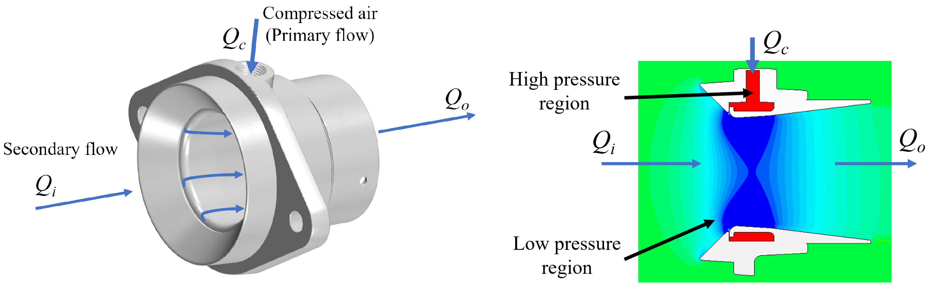
Regardless of how the primary flow is generated, the working principle of air amplifiers is the same. On air-supplied air amplifiers, the process is as follows: The high-pressure flow is first injected into an annular chamber near the inflow region (see Figure 1), where it is distributed and reoriented for its ejection through a thin ring gap at high speed, producing the high-momentum primary flow. This high-speed jet is expelled towards the intake surface, where it adheres due to the Coanda effect. Essentially, the Coanda effect is the tendency of a fluid jet to induce a low-pressure region in its surroundings, leading to the entrainment of nearby fluid. When the jet flows in proximity to a surface, the entrainment of fluid between them generates suction, deflecting the jet over the surface to which it remains attached. This effect also enables the jet to follow adjacent curved surfaces, as in the case of the air amplifier. Subsequently, the jet expands towards the outlet. As a result of this flow expansion, a low-pressure area is created in the inflow region, which induces a high-volume entrained air flow into the amplifier chamber, the secondary flow. The combination of primary and secondary flows is directed towards the outlet of the device, providing the so-called “amplifier effect” with respect to the injected primary flow.
In terms of an analysis of their performance, several works that address the impact of the main geometrical parameters on the performance of air amplifiers can be found in the literature, most of them from a numerical approach. There is a consensus that the most critical parameters are the width of the injection gap, , and the total pressure of the injected air [1,11,13,14,15,18,20,21,22]. The higher the injected air pressure, the higher the primary and secondary flow rates. Regarding the gap width, there is an optimal value that maximizes the amplifier factor. A variable gap width controlled by piezoelectric actuators is analyzed to achieve an optimal gap width. Other geometrical parameters have also been investigated, in particular [23] focused on the influence of the air amplifier outlet diffusion angle, together with the sensitivity of the device performance to the aspect ratio of inflow and outflow areas.
Some of these numerical approaches have been supported by an experimental measurement of flow observables on commercial air amplifiers that are in operation. Among other works, several pressure transducers and a flow mass meter were used in [22], while the authors in [14] supplemented the static pressure measurements with a particle image velocimetry (PIV) analysis of the flow field.
The variability and sensitivity of the geometrical parameters are not negligible and require a combination of experimental and numerical data for a robust correlation of the results obtained. In addition, the aforementioned works have focused on the characterization of air amplifiers that work isolated or in “blowing mode”, that is, to provide a uniform jet flow. The potential of these devices operating in ”suction mode”, as some manufacturers recommend [24], has not been fully investigated. In this work, a combination of numerical and experimental techniques is employed to characterize a commercial air amplifier device, exploring three operating conditions (isolated, “blowing”, and ”suction” modes) and the influence of direct geometrical scaling of the device, while keeping the injection gap and pressure line limitations. Volumetric mass flow rates are obtained experimentally by means of an internationally standardized flow meter, ensuring the replicability of the results.
2. Air Amplifier Setup
The industrial air amplifier considered here is the EXAIR Super Air Amplifier 120024, hereinafter referred to as ESAA. The ESAA is made up of two separate body parts that, when assembled, create a cylindrical duct. The first, on which the external fittings are mounted, contains the inlet section of the duct and a screwed intake for the pressurized flow, connected to an annular stagnation chamber that ends in an annular slot. The second part is screwed into the first one, allowing for an adjustment in the aperture of the aforementioned slot (see Figure 1).
The following sub-indexes are used to identify the different sections: is the inlet amplifier section, is the outlet amplifier section, and is the compressed air inlet section. The reference frame is mounted on the axisymmetric axis of the circular section of the secondary flow of the amplifier.
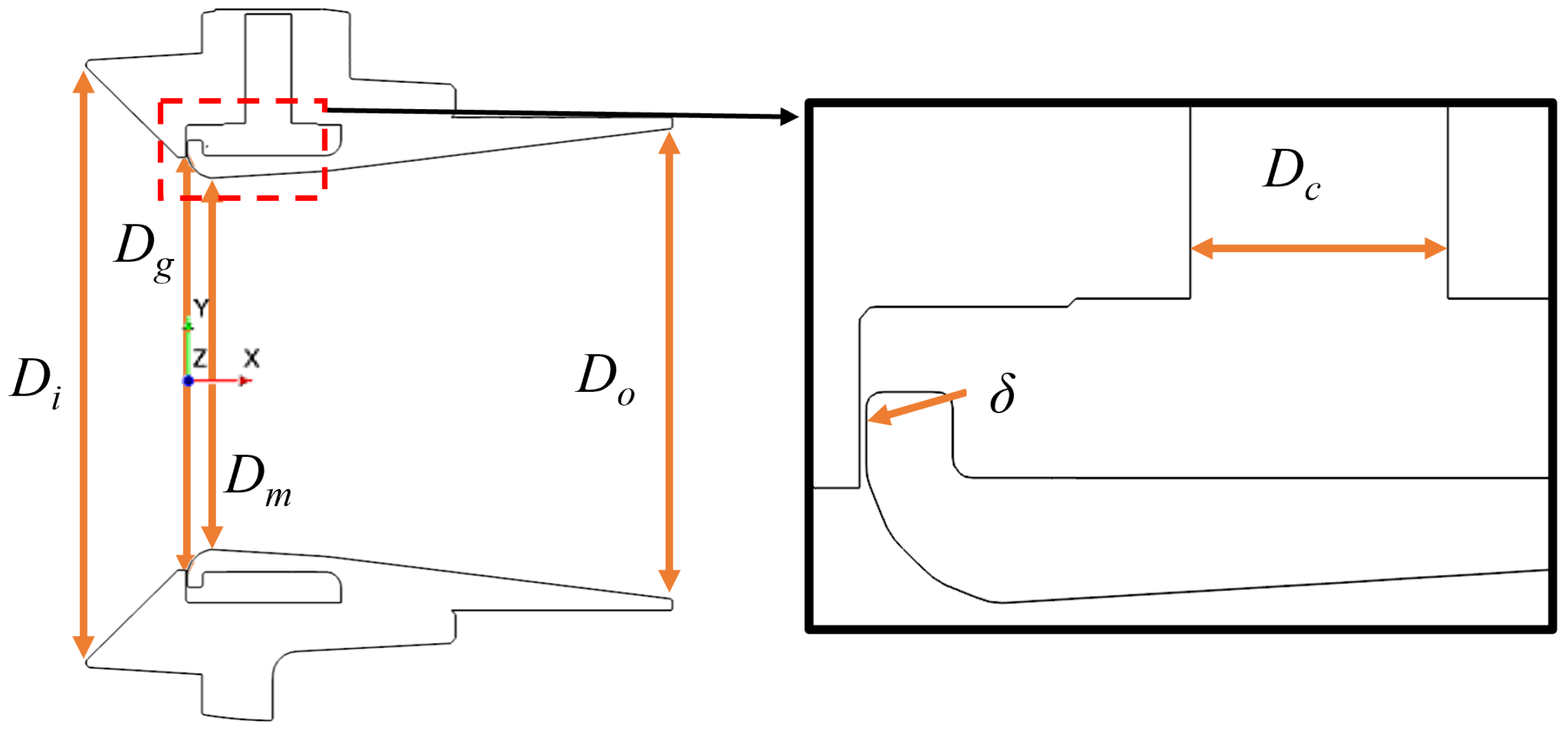
As sketched in Figure 1, two inflow sections and one outflow section are identified. A primary pressurized flow characterized by its volumetric flow rate and static pressure ( and , respectively) is first introduced into an annular chamber through the compressed air inlet section, , with an inner diameter . This primary flow is then accelerated through a thin ring nozzle, the aperture of which is defined by the gap parameter . The flow is tangentially ejected, remaining attached along the intake thanks to a Coanda profile, which directs the flow to the outlet, preventing boundary layer separation. Transfer of momentum from the primary jet flow towards the axis of symmetry occurs through viscous effects, and a low-pressure area is created at the center line of the inlet section , with diameter . This pressure drop produces an entrainment of induced flow rate, . The combination of the two incoming flows results in the formation of the secondary flow, which is expelled through the outlet section , with diameter , at a flow rate of . Downstream from the outlet section, secondary and primary flows are mixed due to the persistence of a high turbulent intensity. The clearance distance that defines the Coanda nozzle gap, , is one of the critical parameters in the geometry of the air amplifier (see Figure 2), as it can limit the injected mass flow due to blockage effects (this is elaborated in Section 5.3.1). Main dimensions are depicted in Figure 2. Axis X is aligned with the axis of symmetry and the main direction of the flow, and Y and Z define the main aximuthal plane. Two additional parameters are defined to characterize the air amplifier: the minimum diameter of the section in the secondary flow area, , and the diameter of the section where the Coanda nozzle is located, , with this last one being used to compute the non-dimensional mass flow. The main dimensions of the air amplifier model used are listed in Table 1.
The performance of an air amplifier is usually measured by the volumetric flow rate (or amplification factor) as . The amplification factor reflects the impact of the primary flow on the entrainment of the secondary flow and can be complemented by the mass flow rate measured in the outlet section or the outflow mass flow rate as follows:
where is the air density in the respective section indicated by the subscript.
The flow regime remains defined by the Reynolds and Prantdl numbers. The local Reynolds number in a characteristic section may be defined by the passing massflow, , and the section diameter, D:
where is the fluid viscosity. The Prandtl number is defined as follows:
where is the specific heat capacity at constant pressure and k is the air thermal conductivity computed through the Sutherland’s law. All parameters consider a constant reference temperature. In what follows, a constant value of was considered. While varying depending on the flow velocity across the air amplifier, the Reynolds number based on the inner diameter of the device takes values of . Finally, the Mach number is defined as follows:
where U is the velocity magnitude and is the speed of sound.
Depending on the pressure boundary conditions, as the primary flow follows the curved surface of the Coanda profile, expansion and compression waves might appear; consequently, flow compressibility effects should be considered. In this regard, the non-dimensional mass flow through the Coanda nozzle is monitored to study blockage effects, given by the following expression:
where R is the gas constant; is the reference temperature; is the compressed air pressure; and is the area of the Coanda nozzle throat, which represents the minimum cross-sectional area at the Coanda nozzle.
Mass Flow Measurement Procedure
On the evaluation of the entrained flow, , which ultimately defines the amplification factor of the device, several methodologies can be used. Measurement of internal or volumetric mass flows is normally carried out by industrial devices, via mass flow meters of different kinds. However, empirically determining the flow entrained by the air amplifier carries additional complications. In circular-section ducts, an appropriate acquisition of pressure data under stationary conditions may be used to accurately calculate the mass flow going through the duct. With this aim, a contraction on the duct is installed down/upstream from possible perturbations, forming a so-called “Venturi-tube”. The Venturi-tube is formed by a conic-convergent section, followed by a straight cylindrical part, and finally connected to a conic-different section. The dimensions and measurements of these sections are not arbitrary. In particular, in this work, the Spanish UNE-EN ISO 5167 standard [25] has been followed. This standard establishes the general principles for the measurement procedures and mass flow calculations, defining the requirements, dimensions, and installation of a Venturi-tube for measurement, together with the limits for the flow conditions and tube dimensions.
The contraction of the Venturi-tube is preceded by a long constant section pipe, along which static pressure taps are strategically placed in a cross pattern (see Section 3.3). The pipe connects to a diametrical section contraction in which the flow is accelerated and the static pressure is measured at its lowest value, allowing for the pressure drop generated by the contraction to be obtained. The flow and pipe characteristics, together with the corresponding pressure drop values, can be used to determine the mass flow that passes through the contraction following the UNE-En ISO 5167 standard.
Combining the mass flow measurements at the Venturi tube contraction with instrumental data from the high-pressure line of the air amplifier, the amplification factor of the device can be characterized and evaluated.
Finally, for repeatability and a better comparison of numerical and experimental results, we clarify the units used for the volumetric flow rate in this work. Standard liter per minute (SLPM) is a unit of volumetric flow rate of a gas at standard conditions for temperature and pressure (STP), which is most commonly practiced in the United States, whereas European practice revolves around normal liter per minute (NLPM) units. The conversions between each volume flow metric are calculated using the following relations:
Equation (6) can be reformulated to be based on the flow density, as follows:
3. Experimental Setup
This section contains a description of the experimental setup used to characterize the three air amplifier configurations tested: blowing, suction, and isolated. Its content is divided into five parts: a description of the high-pressure line used to feed the air amplifier, followed by the manufacturing and assembly details of the Venturi tube, and ending with three subsections regarding the instrumentation setup used during the experiments on the different analyses and the air amplifier airflow adjustments.
3.1. Primary Flow Pressure Line
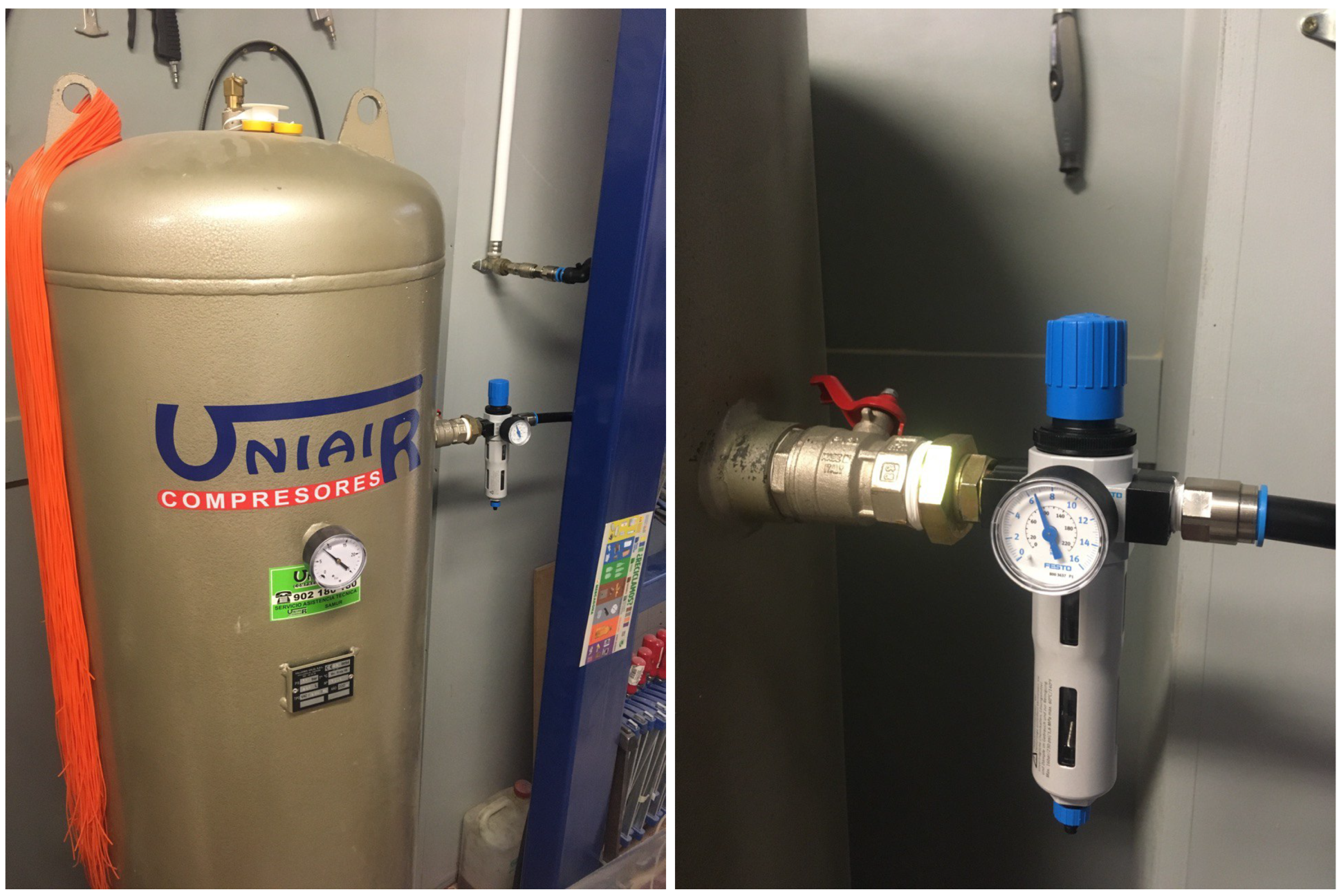
The experiments were carried out at the Montegancedo Campus facilities of IDR/UPM. A high-pressure line was installed along the different sections of the facility, fed from a reservoir tank with adjustable output pressure, and maintained by an air compressor (see Figure 3). The reservoir tank has a volume of 300 L, compressing the enclosed air to 9.5 bar. A pressure regulator device equipped with an air filter is located at the outlet of the tank, ensuring constant output pressure during the use of compressed air. Quick-release fittings located along the facility allow for the connection and use of the line for the instrumentation and hardware needed to build and run the experiments for the models during the aerodynamic analyses.
Constant-diameter fittings and an internal diameter of the piping of 15 mm were used, reducing the length of the tubing to approximately 2 m. Ending the piping, instrumentation was installed to characterize the high-pressure flow feeding the air amplifier:
- A PFD-202-20 volumetric mass flow measurement device, with a flow rate range from 100 to 2000 NLPM and a diameter section of 15 mm, was chosen to determine the mass flow entering the air amplifier. Following the specifications of the air amplifier manufacturer, a maximum volumetric mass flow of 700–800 NLPM was expected. The PFD-202-20 was designed for clean compressed air, has a resolution of 5 NLPM and a maximum operating pressure of 1 MPa, and allows for cumulative flow rate measurements. Measurements are given in NLPM units.
- A ball valve (with minimal pressure loss when fully opened) was placed downstream from the flow measurement device, ensuring that no disturbances were made on the measurements.
- A CKD digital pressure sensor (PPX Series) provided static pressure measurements at the high-pressure inlet of the air amplifier.
In the calculations of the mass flow rate, a constant room and reservoir temperature was assumed. The density of the compressed and entrained flow was thus calculated by assuming air as an ideal gas and only dependent on the local pressure, considering isotropic gas expansions.
3.2. Manufacturing and Assembly of the Venturi Tube
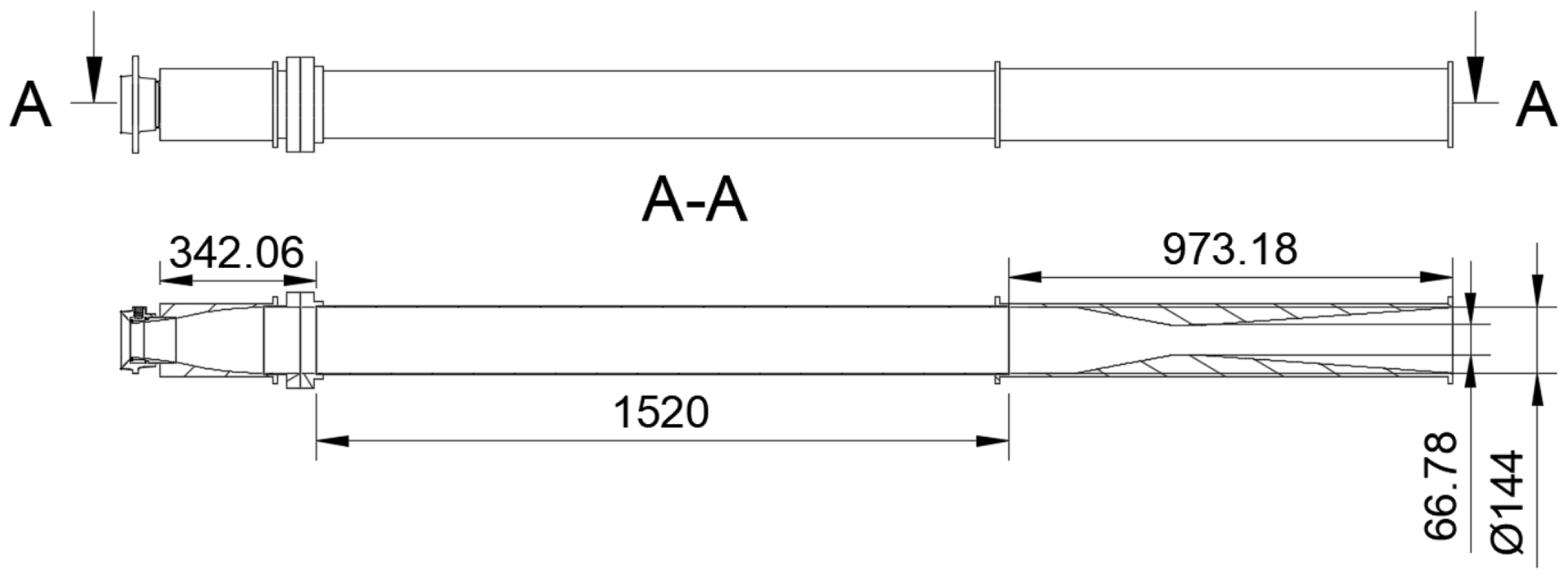
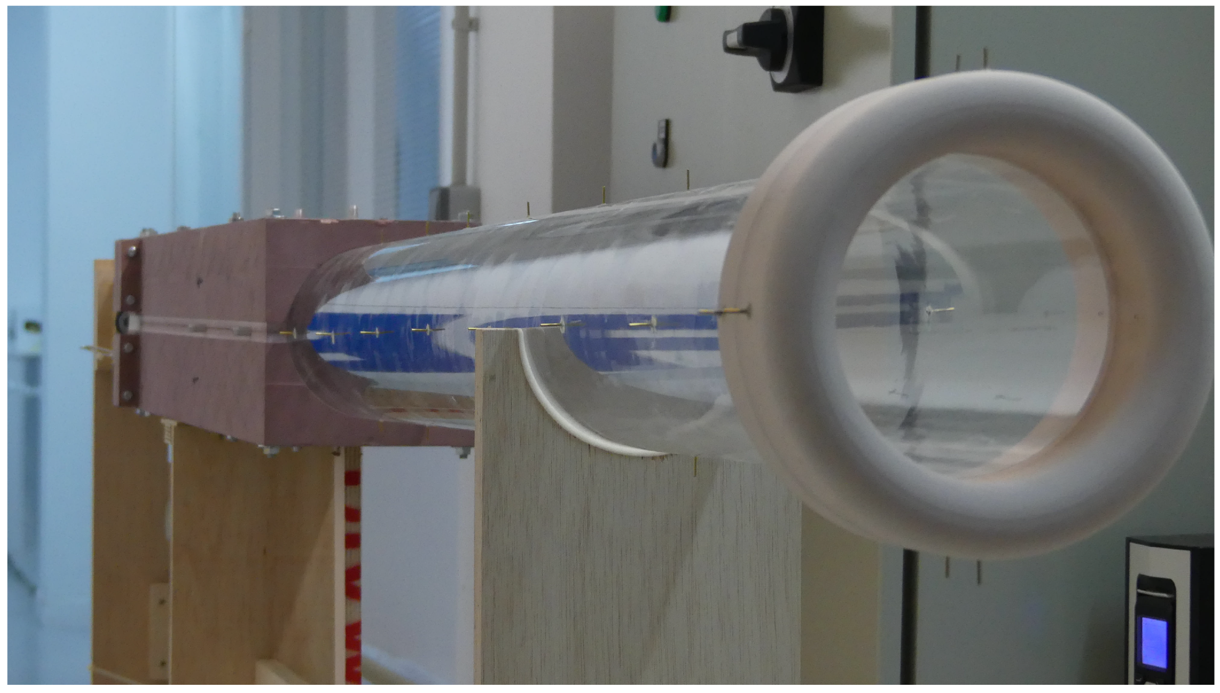
The Venturi tube used to measure entrained flow adheres to the UNE-En ISO 5167 standard, with its key dimensions detailed in Figure 4. In accordance with these standards, it is required to establish a distance upstream from the constriction to ensure uniform and attached flow conditions. Consequently, a constant cross-section pipe was positioned upstream from the Venturi location. This section utilizes a methacrylate plastic tube, while the variable cross-sections are milled into Necuron, a high-density polyurethane material with excellent physical properties (see Figure 5, Figure 6).
Two additional parts were custom-designed and computer numerical control (CNC)-milled in Necuron to properly fit the air amplifier up- or downstream from the Venturi, to evaluate the two different working configurations of the device. The operating setup of the blowing mode, where the air amplifier is located upstream from the Venturi tube, and the suction mode, where the device is placed downstream from the restriction, are depicted in Figure 7. Each additional part is attached to the tube only when fitting is required.
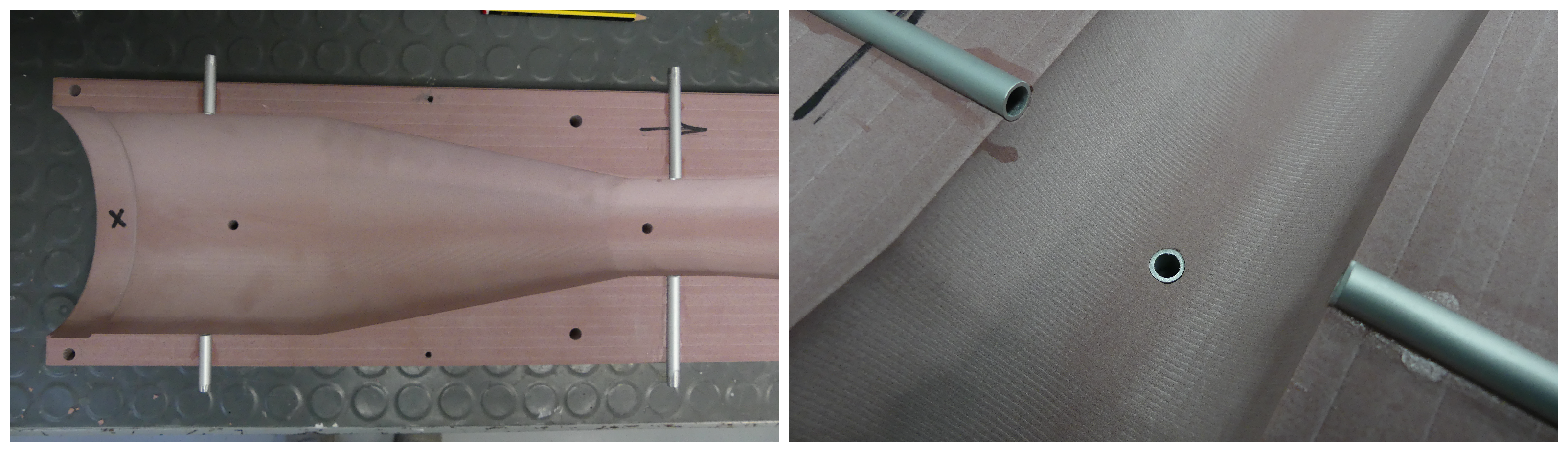
The UNE-En ISO 5167 standard not only provides dimensions for the maximum wall angle or constriction distances but also provides specifications for the pressure tap diameter inside the Venturi tube constriction. As shown in Figure 8, larger diameter inserts were placed where the pressure tap would be located, ensuring proper measurement of the inner pressure in the tube.
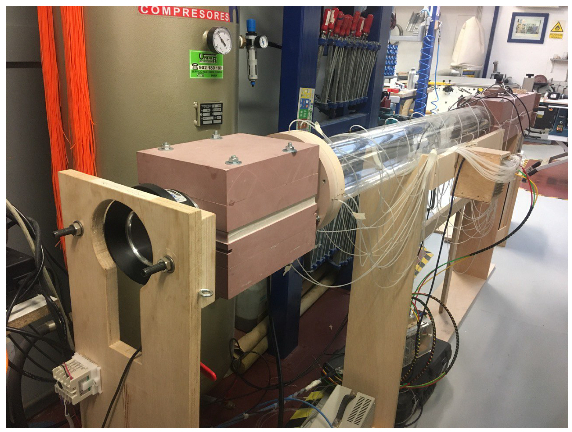
The final assembly was mounted on a rigid structure that kept the different parts aligned and in place throughout the experimental campaign, also facilitating the repositioning and adjustments needed on the air amplifier for the different analyses. Figure 9 shows a general view of the entire setup during the experiments.
3.3. Venturi Tube Instrumentation
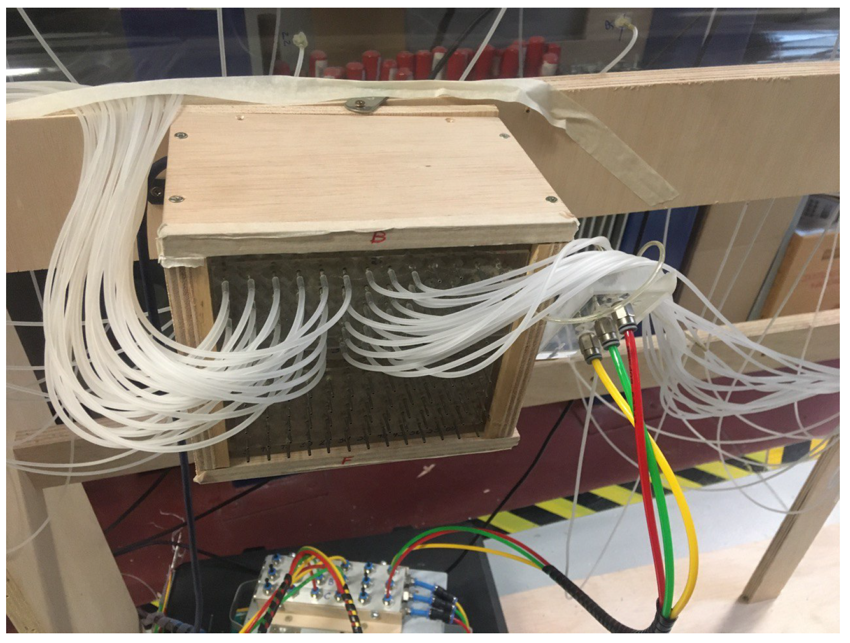
A total of 44 pressure taps were placed along the methacrylate tube and the Venturi tube constriction, to evaluate the mass flow through the air amplifier and to provide reference data for numerical correlation. The taps were distributed in ten stations in groups of four along the tube and Venturi, allowing the averaging of the pressure values at each station. Each pressure tap was connected to a hydraulic line and finally connected to the data acquisition system. The lines all had the same lengths, which were minimized to avoid data interference. The data acquisition system consists of an electronic pressure scanning module (model ZOC33/64PxX2, from SCANIVALVE Corporation), with a maximum range of 2.5 kPa and an accuracy of 0.15% (of the full scale). The pressure acquisition setup is shown in Figure 10. At each experiment, 4000 samples were taken at a rate of 200 Hz, providing 20 s of testing time. The acquisition was started before the opening of the valve to capture the transient effects and to evaluate the stabilization of the flow inside the Venturi tube at each analysis. Further post-processing was required to select an appropriate window of the acquired data to perform a time-averaging and statistical analysis.
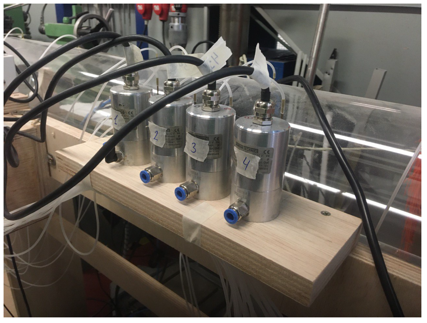
Additional pressure transducers were installed to measure the pressure difference in the constriction section. Four Sensor Technics differential pressure transducers (see Figure 11) with a maximum range of kPa, ran simultaneously with Scanivalve sensors to provide data on the pressure drop/jump across the Venturi tube in all tested configurations.
3.4. Wake Velocity Measurements
The velocity profile of the wake was explored using constant temperature anemometry (CTA) of a vertical array of points, repeated at several downstream locations of the isolated air amplifier. CTA is a measurement technique based on the cooling effect of a flow on a preheated body [26]. On the basis of a previous and accurate calibration (which considers the probe mounting and cables used on the analyses), CTA provides high-precision continuous velocity time series. In these analyses, a triaxial hot wire probe (DANTEC DYNAMICS 55P95) was used to measure velocity components on a three-axis reference system. The hot wire probe can acquire data at frequencies up to 400 kHz, with minimum and maximum speeds of 0.05 and 200 m/s, respectively.
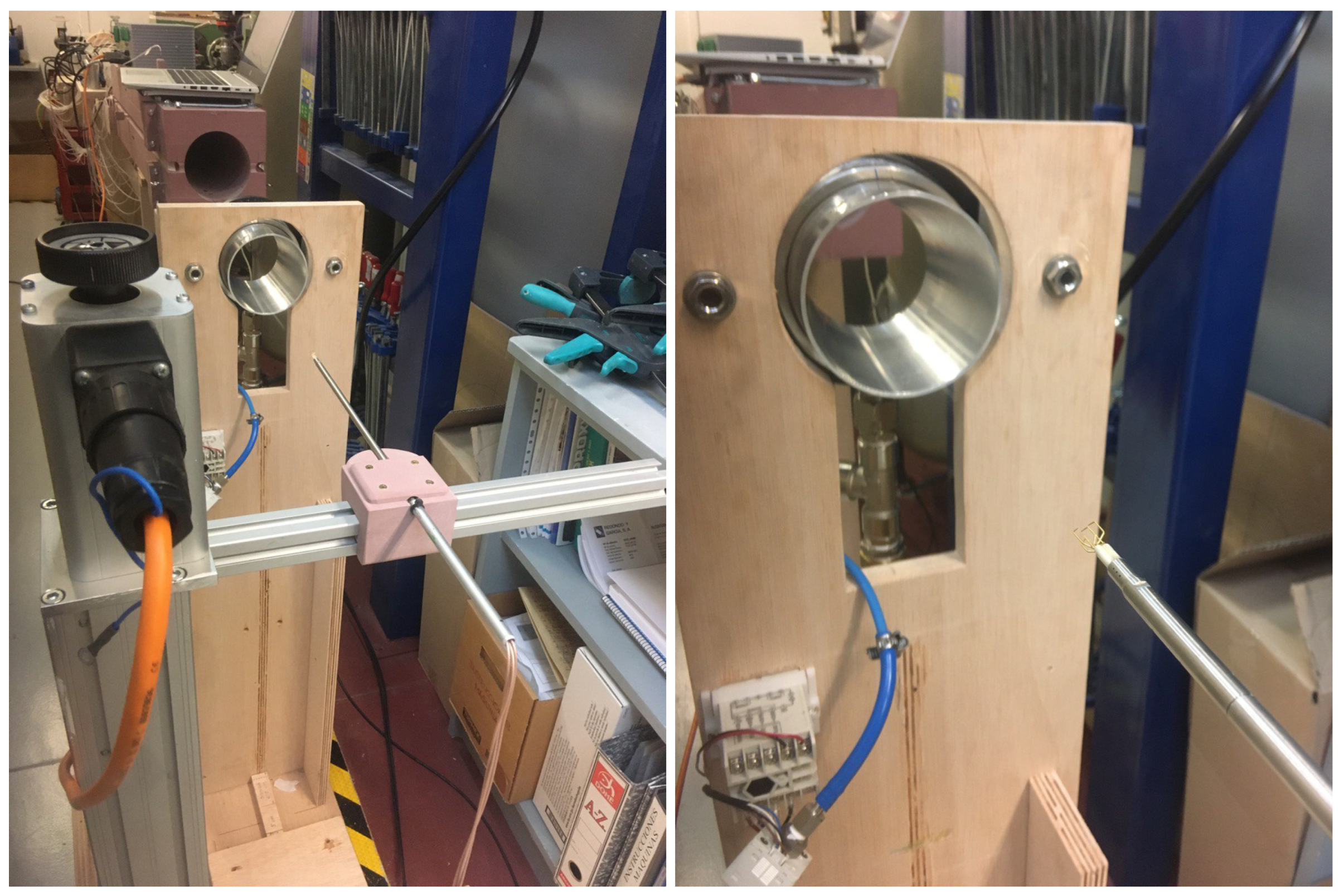
The probe was fitted to a DANTEC DYNAMICS probe support and attached to an ISEL one-axis positioning system (see Figure 12), which is remotely controlled with a location precision of . The positioning system setup was explicitly manufactured for air amplifier analyzes, ensuring adequate positioning of the ISEL system at the different downstream positions of the wake.
The Coanda nozzle gaps were manually adjusted to 0.23 mm, 0.15 mm, and 0.08 mm, following the gap apertures suggested by the manufacturer. This was achieved by using feeler gauges and careful manual adjustment of the screw. In these analyses, the expected uncertainty of the gap value, given by the gauge tolerances, was on the order of 0.01 mm.
Varying the total pressure upstream from the pressure line, a compressed air pressure variation was analyzed, with an approximate range (varying between the different gap configurations) of the total pressure at the air amplifier inlet from MPa to MPa. Note that the upper limit of the pressure range differs from the numerical analyses, as it was limited by the facility constraints.
4. Numerical Methodology
The numerical simulations were performed with the CAD geometry of the ESAA obtained through a reverse engineering process, consisting of a 3D model scanner with a Handyscan Black Elite device. Once the point cloud data were gathered, additional polygonal meshing was performed to define the CAD model surfaces.
The performance of the air amplifier was evaluated for a wider range of pressurized flows, ranging from MPa to 1 MPa. Additionally, we analyzed different geometric parameters to evaluate the technical feasibility of the air amplifier to achieve a higher entrained flow.
4.1. Governing Equations and Boundary Conditions
Let us consider the steady three-dimensional turbulent compressible fluid equations, closing the system with the turbulence model [27]. This eddy viscosity turbulence model has provided very good results when comparing the numerical data with the experimental data of air amplifiers [13,22], although other authors [14] have successfully implemented the Realizable model [28]. Additionally, assuming the air as an ideal gas (i.e., ), the continuity, momentum, and energy equations for a steady, compressible, and turbulent flow are as follows:
where is the fluid density, is the fluid velocity in the i direction, p is the fluid pressure, is the turbulent deviation of the fluid velocity, and T is the fluid temperature. Compressibility effects cannot be neglected, and thus, the energy equation cannot be decoupled from the mass and momentum equations.
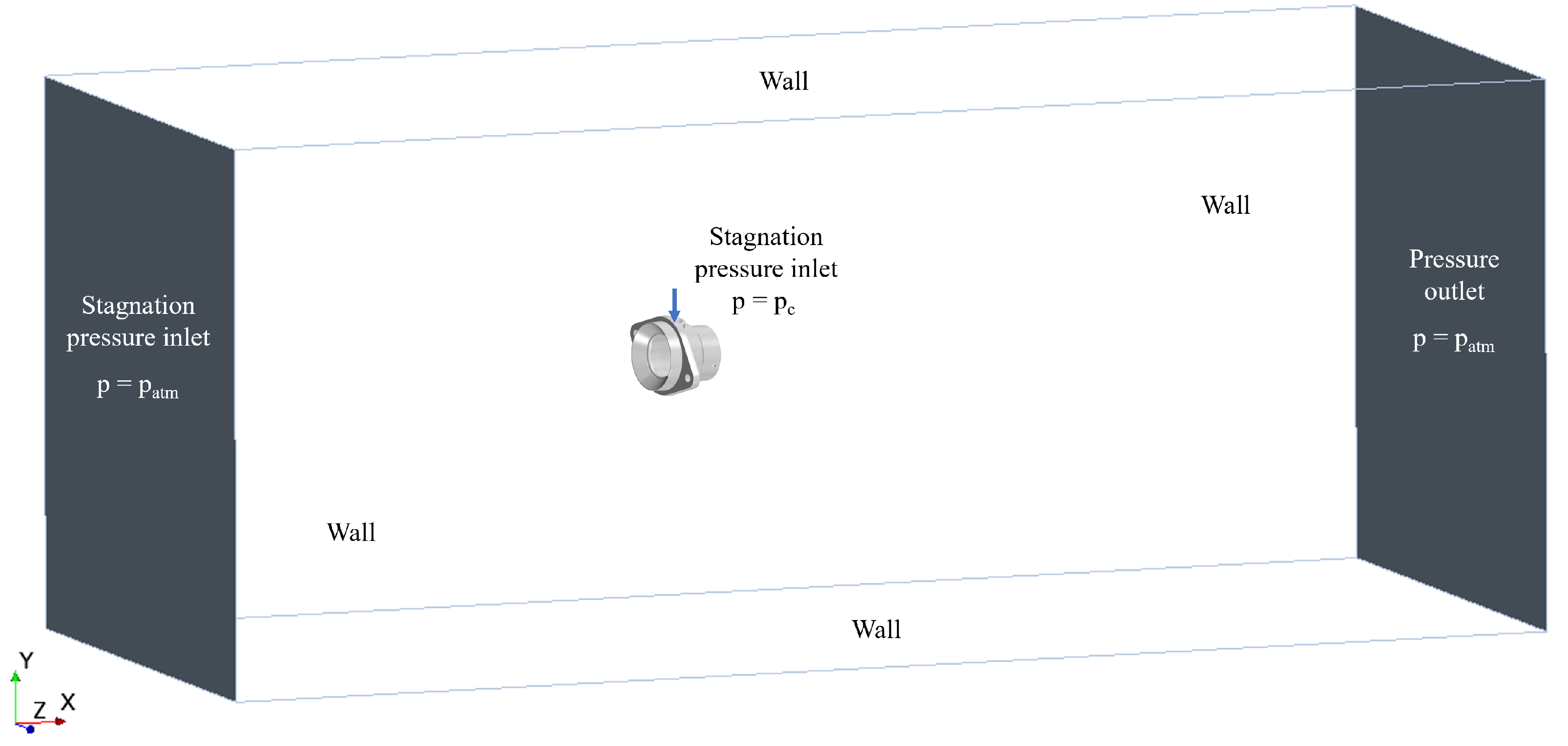
The computational domain extends further from the device in all three dimensions to avoid external boundary conditions’ interactions with the numerical results. A schematic description of the volumetric domain for the isolated air amplifier and the far field boundary conditions of the problem is given in Figure 13. The stagnation pressure inlet conditions are fixed upstream from the device, and static pressure conditions are fixed at the outlet, setting an atmospheric pressure, , at both sections. The difference between them is that the inflow is treated as a stagnation section, where the fluid is at rest, while a flow velocity field is allowed in the outflow section. The upper, lower, lateral, and air amplifier walls are solid walls where no slip boundary conditions are imposed. In the suction and blowing configurations, the Venturi geometry is added to the computational domain, where the walls are also imposed as a no slip boundary condition. The pressurized air inlet of the air amplifier is modeled as a stagnation pressure inlet boundary condition, with . Finally, we assume that all boundaries are thermally isolated , with the only exception of the reference temperature of K, which is imposed at the inlet section.
The STAR-CCM+ software is used to solve the stationary fluid problem using finite-volume discretization. STAR-CCM+ is a complete engineering software package capable of solving the compressible Navier–Stokes equations for turbulent flows. A semi-implicit method, known as the SIMPLE algorithm, is used to handle the velocity–pressure coupling of the Navier–Stokes equations and to calculate primitive variables such as density, pressure, temperature, and velocity at the steady state. For these steady simulations, an iterative process is used to ensure that the steady-state condition is satisfied with low residuals.
4.2. Grid Convergence
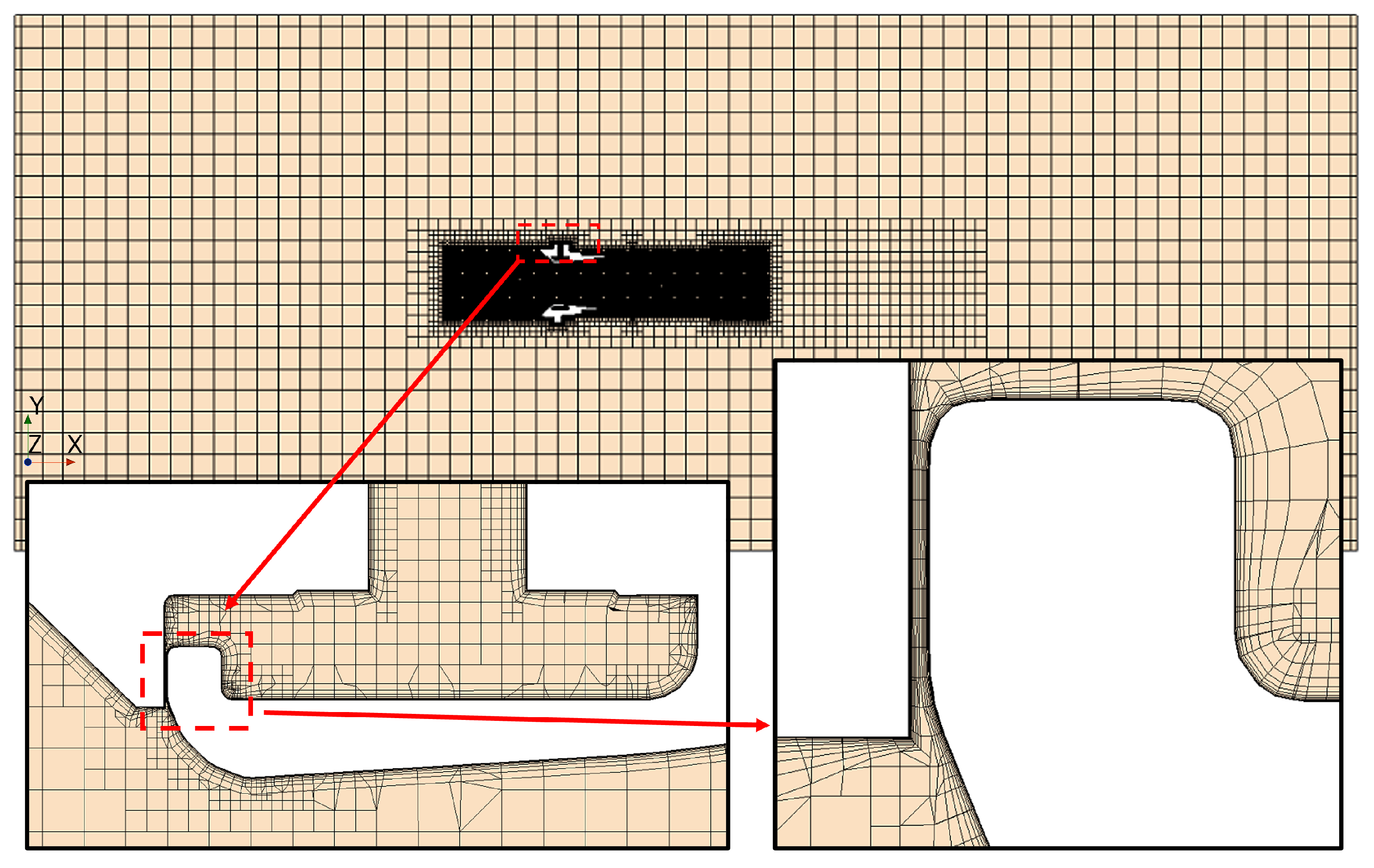
A mesh sensitivity analysis was performed to avoid dependence of the observables (i.e., the amplification factor) with respect to spatial resolution. For this particular study, the compressed air inlet pressure was set at MPa and the clearance parameter was set to = 0.23 mm. Four different hexaedral meshes (named ) were generated, all of them satisfying enough wall normal resolution to comply with a criterion to ensure a proper solution of the full boundary layer. An overview of the spatial discretization, together with a close view of the most conflictive regions, is depicted in Figure 14. The relative error between the different grids is computed with the following expression:
The results of the three-dimensional analyzes are gathered in Table 2. For the two finest meshes, and , the calculated amplification ratio varies below a relative error of 2%. Therefore, to balance the computational load and accuracy demand, grid was used during the simulations.
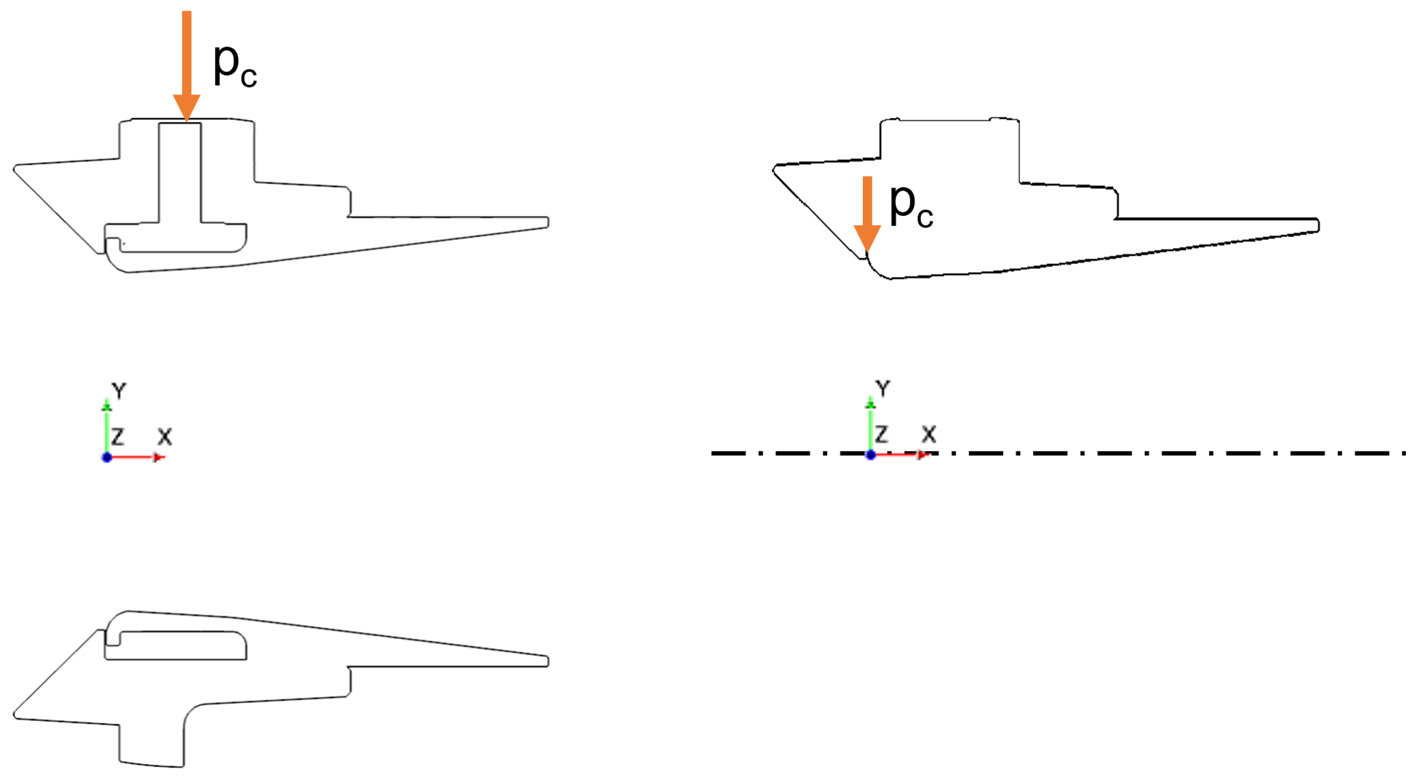
4.3. Axisymmetric Setup
The use of an axisymmetric model is based on the assumption that, above an inlet total pressure of MPa, the air amplifier works under sonic conditions in the injection gap, with the nozzle flow choked. Assuming operational configurations above this value, it can be assumed that the influence of the upstream flow information will not affect the flow downstream from the gap. Thus, eliminating the pneumatic line of primary flow and the inner stagnation chamber of the air amplifier from the numerical simulations allows for a significant simplification of the simulation and hence a considerable reduction in the associated computational cost. Instead of using the three-dimensional Navier–Stokes equations (see Equations (8)–(10)), we use the cylindrical representation of the compressible Navier–Stokes equations, assuming no azimuthal velocity for the axisymmetric flow. The geometry and boundary conditions are similar to those considered in the three-dimensional setup, except that the compressed pressure inlet is located at the injection gap and an axisymmetry boundary condition is applied on the axis of radial symmetry (see Figure 15). This setup allows for faster numerical convergence of the flow solutions and reduced computational time: 48 h (3D model) vs. 0.5 h (axisymmetric model).
This configuration is used in Section 5.3.3 in the study of the sensitivity of the air amplifier performance to the ratio defined by the width of the injection gap, , and the diameter of the minimum section in the secondary flow area, .
5. Results
The results are presented here in four distinguished parts. First, Section 5.1.1and Section 5.1.2 contain the evaluation of the mass flow rate across the air amplifier under downstream and upstream operating conditions, defined in Section 3 as blowing and suction configurations. Subsequently, a correlation between the experimental and numerical data serves as a validation test by comparing the wake profiles produced by an isolated air amplifier obtained during the experimental campaign (Section 5.2), followed by a numerical characterization of the air amplifier performance under different input conditions. A wide range of primary flow pressure values, , and Coanda nozzle gaps, , are explored in Section 5.3.1. With the help of numerical simulations, this study delves into the comprehensive characterization of an air amplifier, with the aim of providing valuable information on its flow patterns, operational parameters, and sensitivity to geometric variations. Finally, the scaling effects of the air amplifier are explored numerically in Section 5.3.3, investigating the limitations and potential of these devices.
5.1. Experimental Characterization
5.1.1. Blowing Mode: Analysis of the Flow Entrained from an Upstream Location
In this configuration (see Figure 7), a Venturi tube-mounted piping system is installed downstream from the air amplifier. The flow is absorbed from the atmosphere and discharged into the straight section of the Venturi tube.
Varying the inlet total pressure coming from the compressed air tank from 0.25 MPa to 0.70 MPa, clearance gap values of mm, 0.15 mm, and 0.23 mm were experimentally analyzed, with a total of 20 operating points collected. The gaps were manually adjusted by employing feeler gauges.
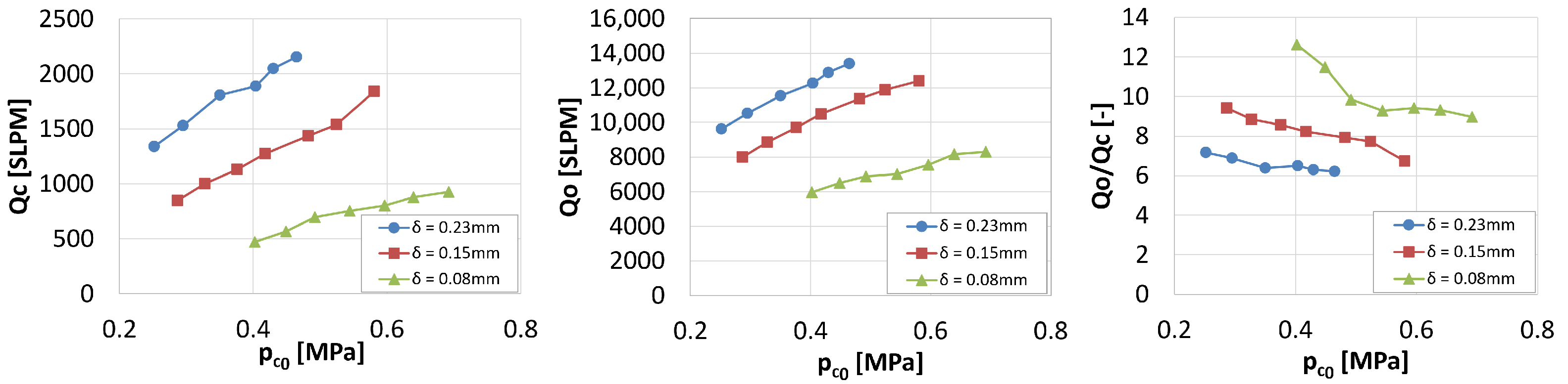
Figure 16(left and middle) depicts, respectively, the high-pressure line and the entrained volumetric mass flow rates, given in SLPM units. According to the results, both mass flows follow a linear trend with respect to the inlet total pressure, together with a direct relation between the mass flow value and the gap width .
Finally, Figure 16(right) reflects the effect of the gap width on the device amplification factor, which tends to increase as the gap decreases. However, the effect of the inlet total pressure is the opposite: the amplification factor decreases with a certain linearity as the inlet total pressure increases until it loses this linearity and remains almost constant. This effect is more noticeable as the size of the gap decreases.
5.1.2. Suction Mode: Analysis of the Flow Entrained from a Downstream Location
In this configuration (see Figure 7), the Venturi tube is fitted with an additional part downstream from the restriction section, in order to fit the upper part of the ESAA, ensuring that only air passing through the Venturi tube is entrained by the device. The flow is discharged to the atmosphere as a free jet.
The inlet total pressure was again varied from 0.35 to 0.70 MPa, and the same clearance gaps were analyzed as in Section 5.1.1. Finally, a total of 18 operating points were collected.
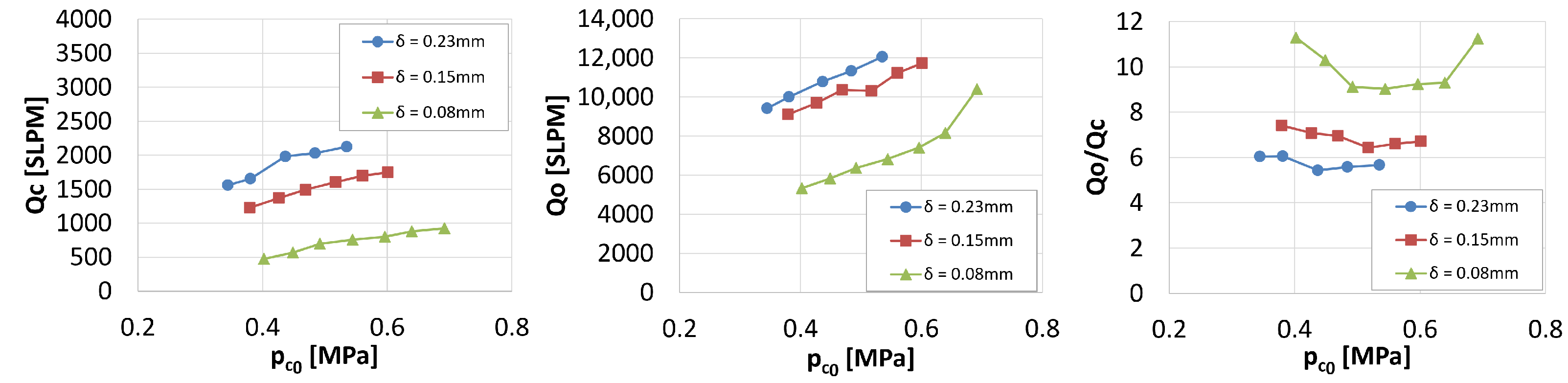
Figure 17(left) reflects the dependence of the injected volumetric mass flow, , on the total pressure provided by the high-pressure line. Differences between configurations with the same gap are believed to be due to the effects of manual adjustment of the screw. Under this operating condition, smaller gaps require a much higher total pressure to provide the same mass flow through the air amplifier.
The aforementioned observations also hold true for the examination of the entrained volumetric mass flow, , shown in Figure 17(middle), where the errors in the manual adjustment of the air amplifier gap seem to have a greater impact than the one observed on the high-pressure mass flow. A linear trend of the entrained mass flow with respect to the inlet total pressure was observed, without signs of mass flow limiting among the evaluated operating points. However, at the last measured point ( MPa), linearity was lost in the entrained volumetric mass flow, which also affected the amplification factor. The results reflect the extreme sensitivity of the entrained mass flow to changes in the nozzle gap, while at the same time show robustness on the performance of the air amplifier, which always maintains the same behavior despite the enlargement of the minimal outflow area.
Finally, Figure 17(right) shows the relation between the entrained and injected volumetric mass flows, also referred to as the amplification factor. Similar to the manufacturer’s tendency [24], the experimental measurements carried out at IDR/UPM facilities show a certain linearity as the inlet total pressure increases until it loses this linearity and remains almost constant. Smaller gaps provide higher amplification factors, reaching values above .
5.2. Experimental–Numerical Correlation
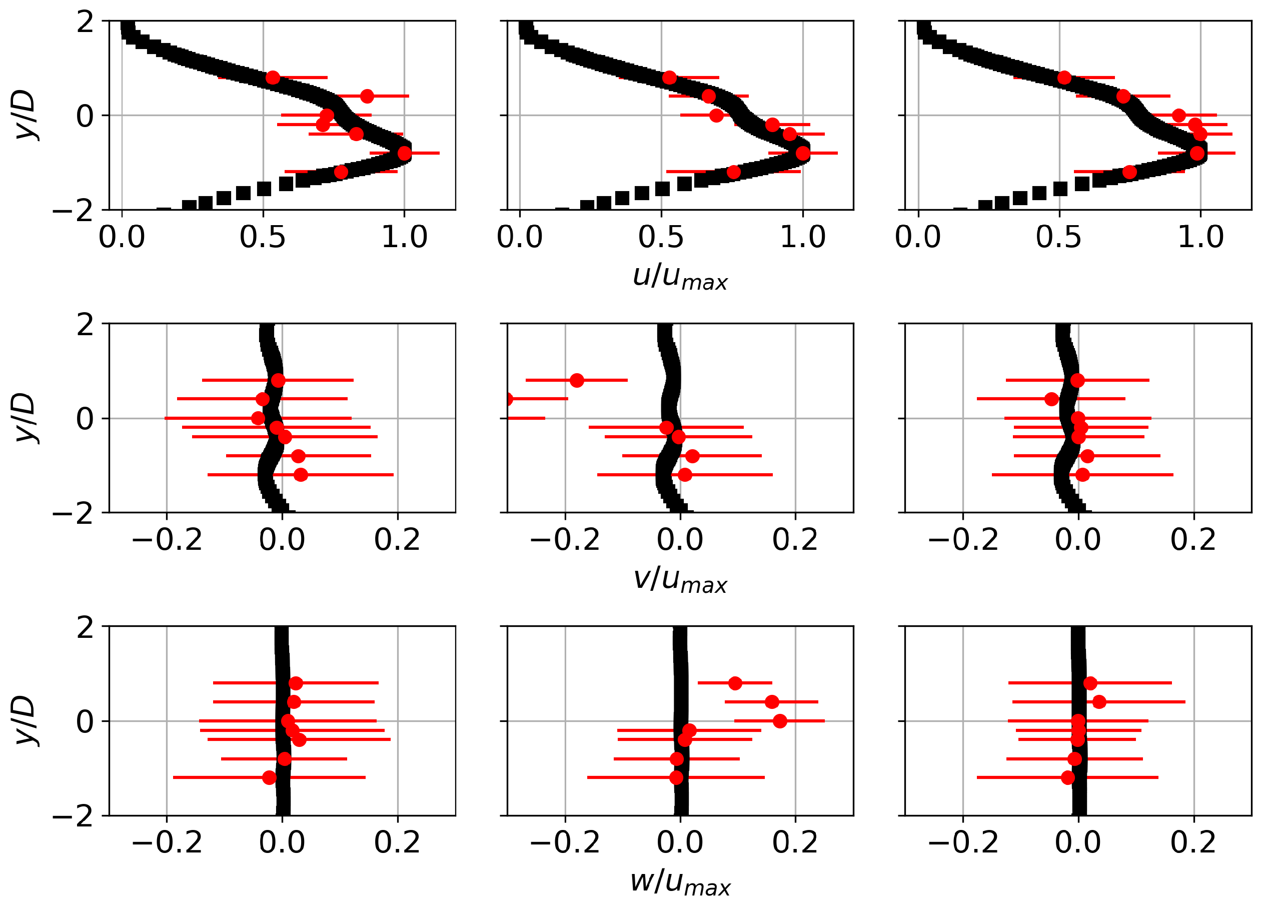
Numerical results in 3D are compared with the experimental data collected by the CTA measurements on a vertical array with seven points of the wake at three different downstream locations located 2.5, 3.5, and 4.5 outlet diameters downstream from the ESAA. Both experimental and numerical results were measured for an isolated air amplifier using a gap of mm and an inlet total pressure of approximately MPa. Figure 18 shows the agreement of the velocity profiles in different sections (, , and ).
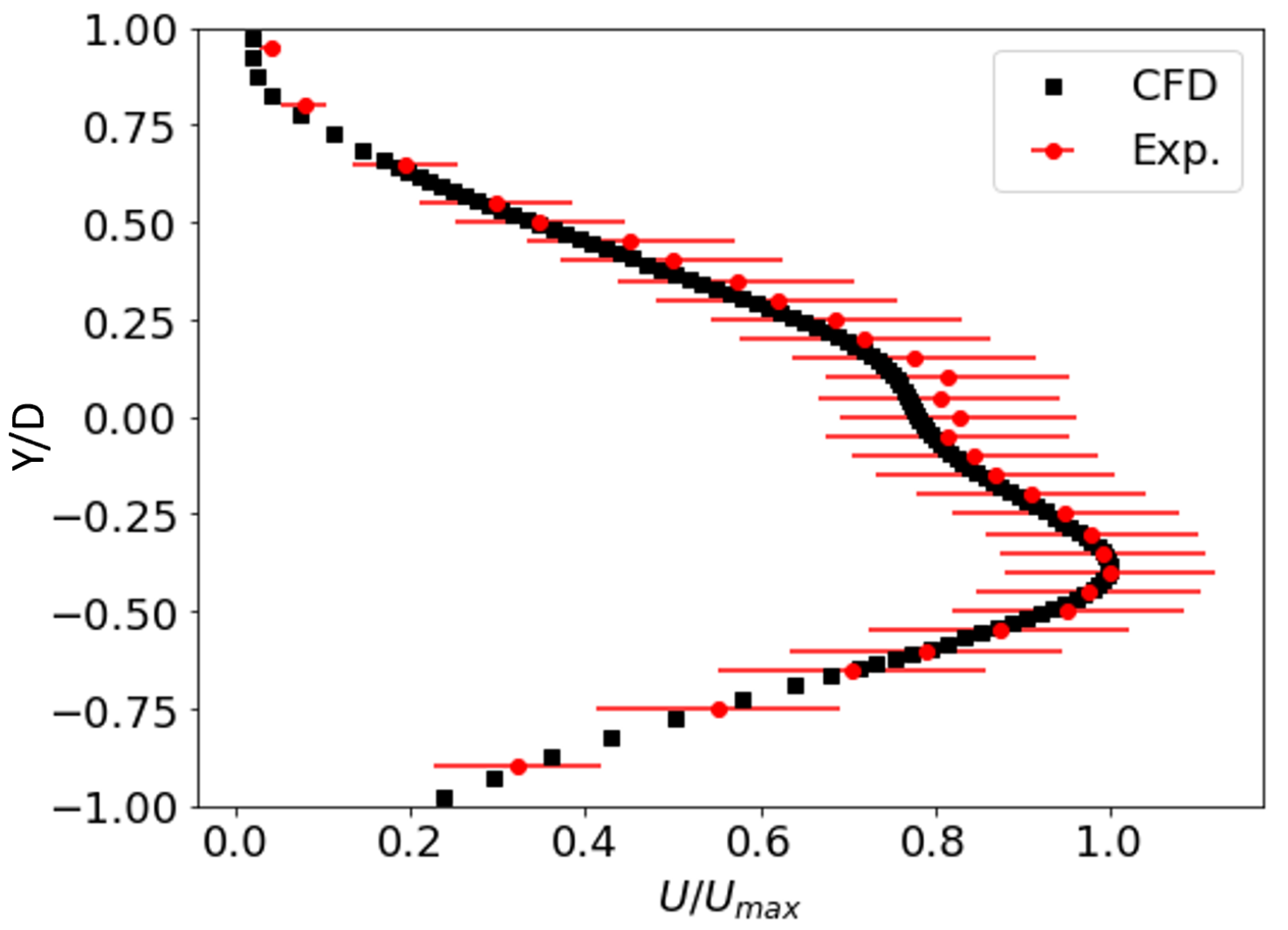
The profiles demonstrate the development of flow asymmetry relative to the central axis, likely attributed to a nonhomogeneous stagnation pressure distribution within the inner ring chamber of the air amplifier. Finally, experimental measurements with further transversal refinement were made in section and compared to the CFD data (see Figure 19), showing a great agreement between the experimental and numerical results.
5.3. Numerical Characterization
5.3.1. Flow Pattern Analysis
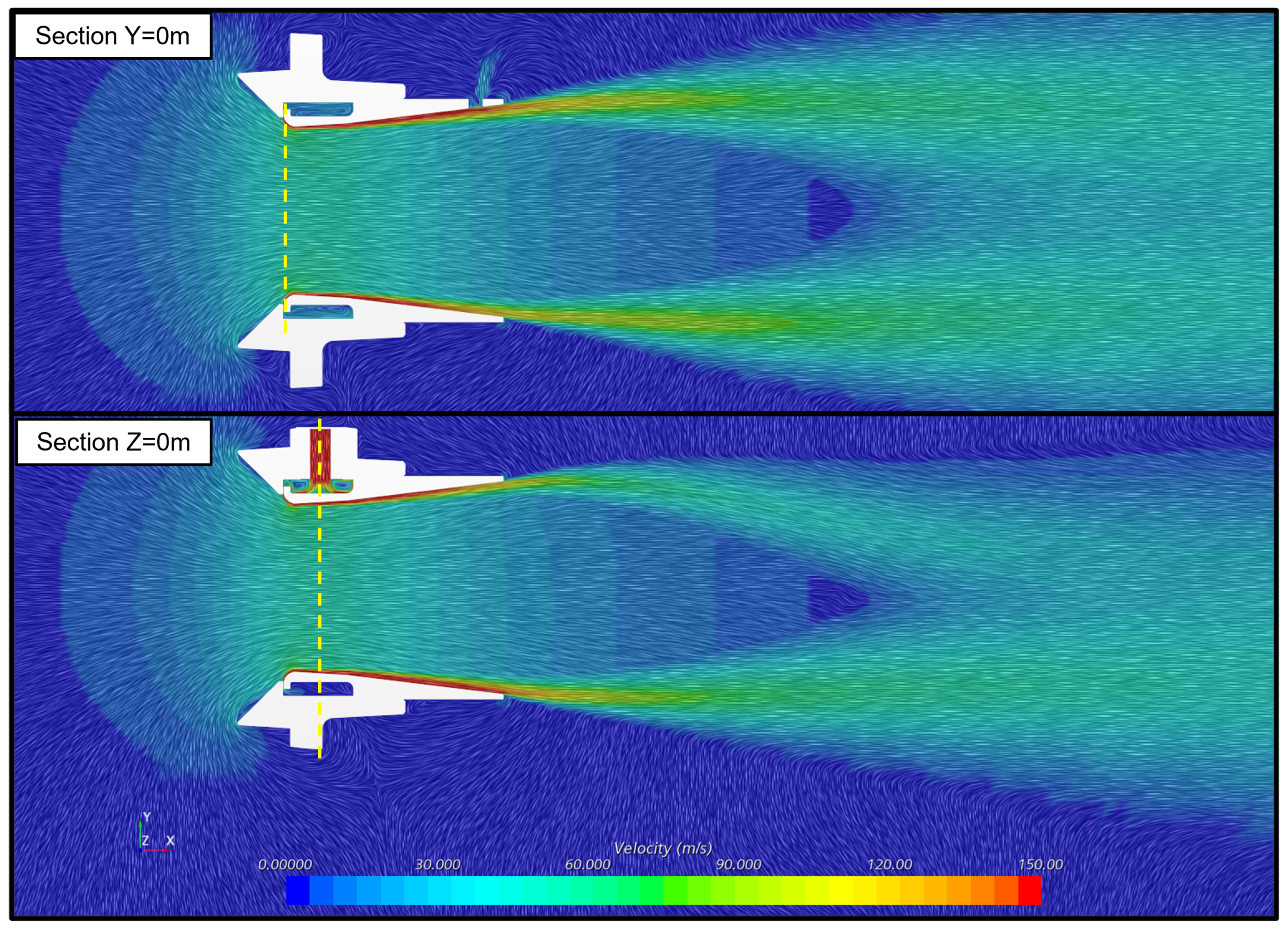
A general perspective of the flow pattern through the air amplifier is shown in Figure 20, where streamline vectors are superimposed on velocity magnitude contours on the planes m (mid-plane of high-pressure line injection) and m (mid-cross-sectional plane). In section m, we found a symmetric flow pattern, dominated by the shear layers caused by the high velocity tangential flow. However, in section m, the flow becomes asymmetric with respect to the central axis, probably due to a non-homogeneous stagnation pressure distribution in the inner ring chamber of the air amplifier. This asymmetry was also observed in the wake profile analyses, as shown in Figure 19.
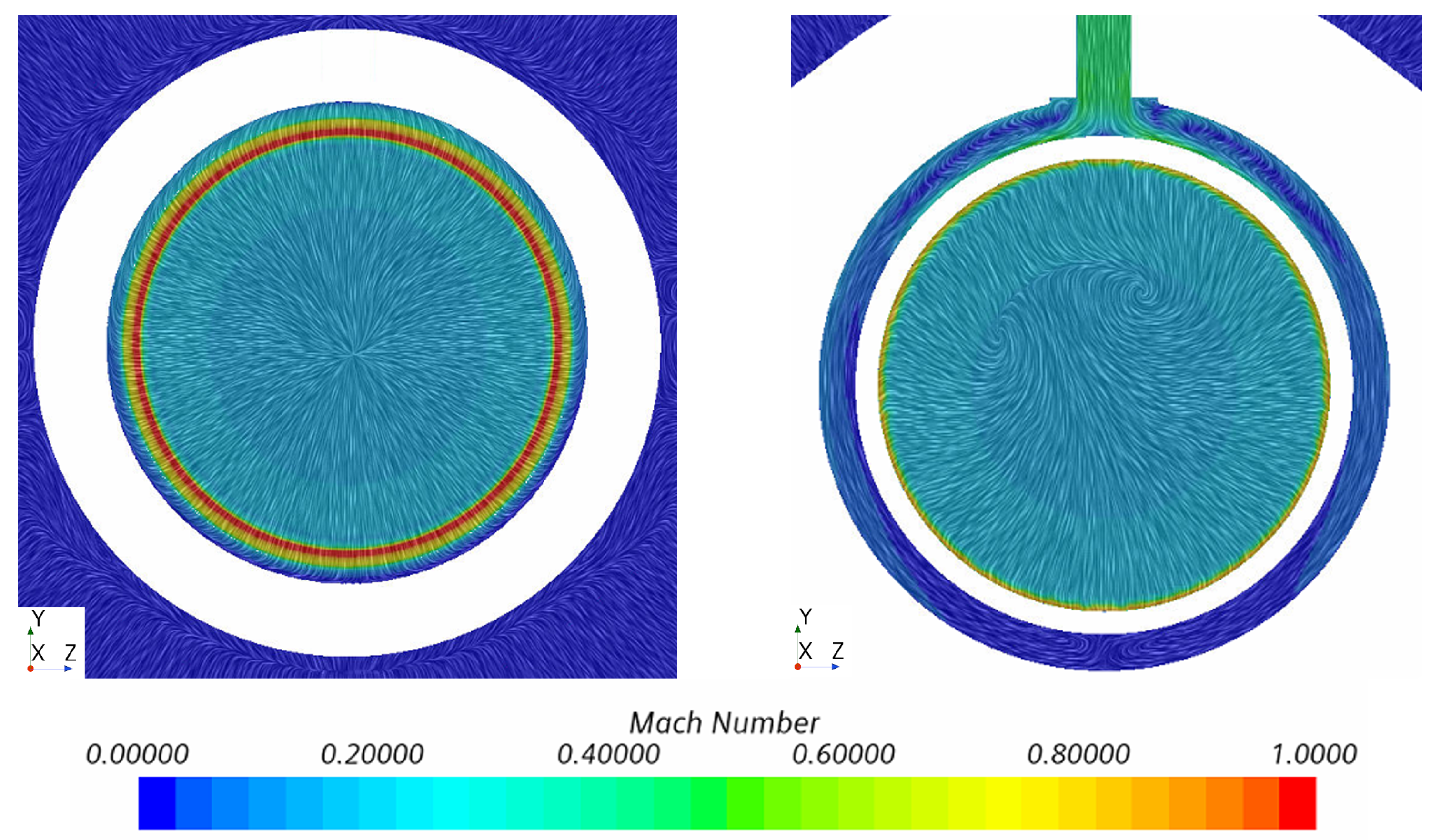
Transverse slides of the flow solution through the air amplifier are gathered in Figure 21 for the planes m and m. The first depicts the flow pattern at the Coanda nozzle gap section, while the latter comprises the primary flow inlet section. A non-uniform velocity profile reflects how the flow progresses along the inner ring producing a non-symmetric flow.
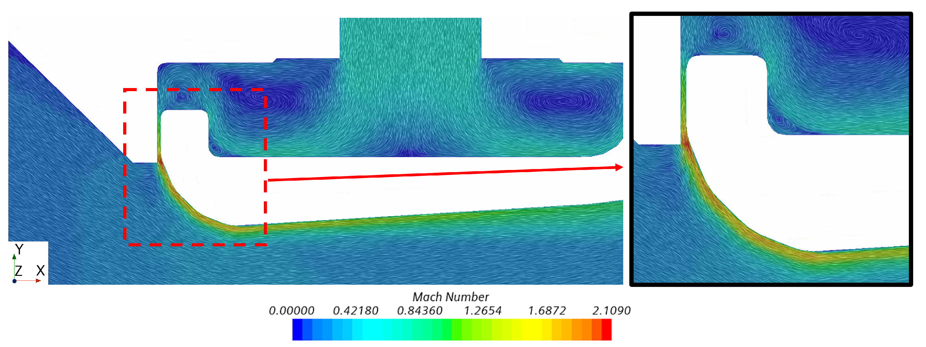
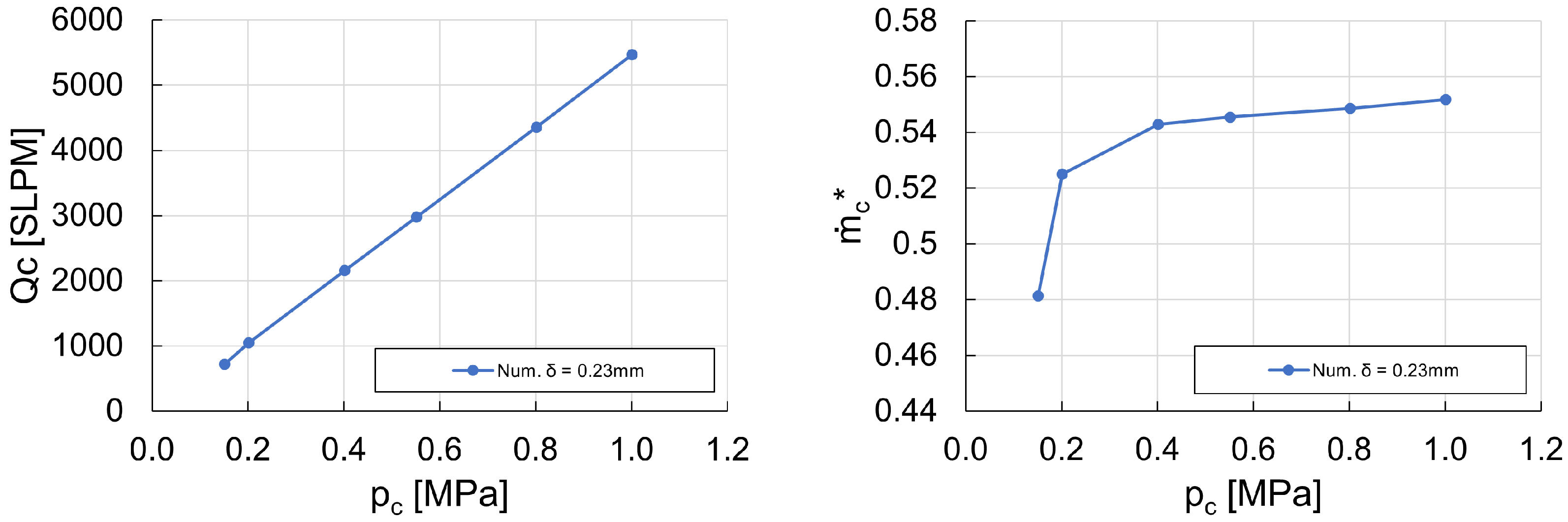
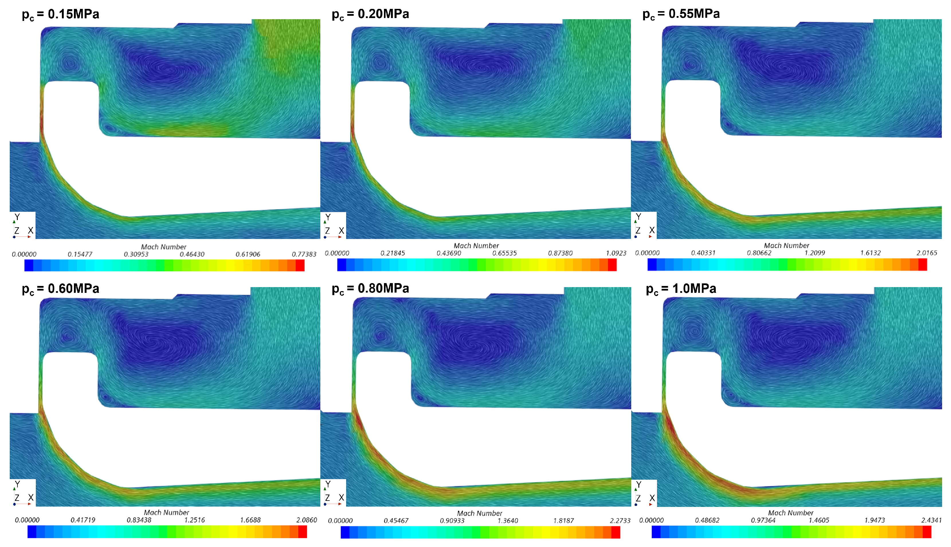
Figure 22 depicts a zoomed view around the injection gap, where the flow through the gap region appears choked near the outlet region. The following increase in the sectional area accelerates the flow to local Mach number values of , with the tangential flow maintaining a supersonic velocity throughout the curved Coanda profile. The effect of this blockage phenomenon is detailed in Figure 23. The linear evolution of the primary volumetric mass flow rate is plotted against the primary flow pressure from MPa to 1 MPa for an injection gap of mm in Figure 23(left), similar to the trend found in the experimental results. However, the blockage effect is shown in Figure 23(right), where the non-dimensional mass flow (see Equation (5)) is plotted against . For small values of the primary flow pressure, there is a large growth in , which finally saturates as a normal shock wave develops in the gap region. Except for the smallest pressure value evaluated, MPa, a region of supersonic flow is observed in the gap region. A clear saturation trend is appreciated, with the non-dimensional mass flow varying approximately by 5% for the pressure range MPa. Note that the saturation achieved is not fully comprehensive due to the impact of viscous effects and the influence of the boundary layer in this confined area. This differs from the ideal flow theory seen in divergent–convergent nozzles, where the saturation is absolute. The development of the supersonic region along the Coanda surface as increases is collected in Figure 24, where Mach number contours for several flow solutions depict the compressibility effects near the gap region.
5.3.2. Analysis of the Effect of the Injection Gap
The analyses performed reveal a high sensitivity of the amplification factor of the air amplifier with respect to the injection clearance gap . This parameter is crucial for the performance of the air amplifier, as it passively limits the flow rate, directly affecting its efficiency.
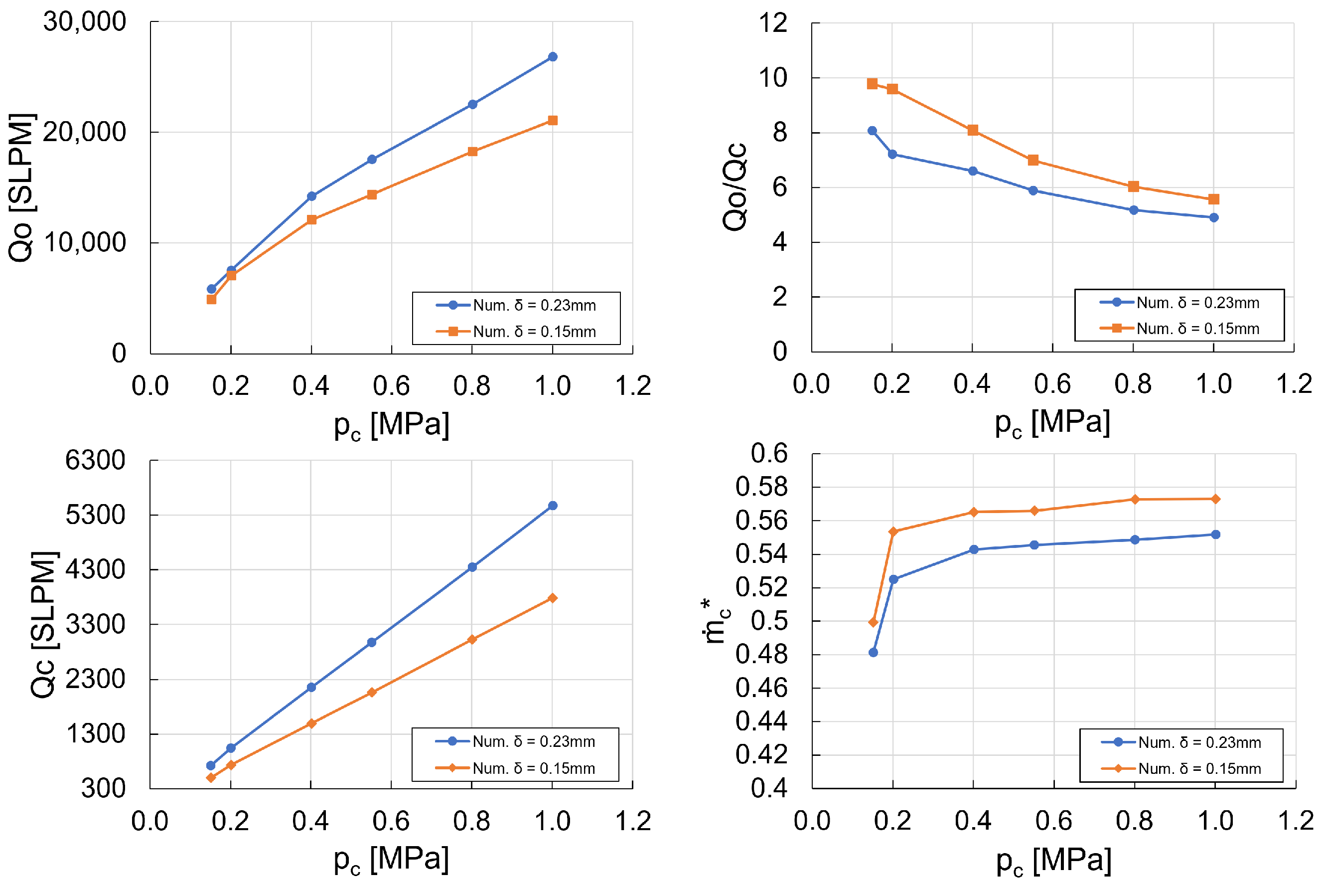
Two different gaps were analyzed, namely 0.15 mm and 0.23 mm. Figure 25 depicts, for both values of , the variation in the primary volumetric flow rate, ; the outlet volumetric flow rate, ; the volumetric outlet/primary flow ratio rate, ; and the non-dimensional mass flow rate, . Note that both volumetric flows decrease with , albeit following distinct trends. A ratio of 1.2 is observed for , while values of 1.5 are recovered for . This difference in ratios provides a higher amplification ratio when the air gap distance decreases. The non-dimensional mass flow rate plots indicate similar blockage effects for both values, saturating as supersonic flow develops in the gap region. Furthermore, with the discretization used, supersonic flow appears in the pressure range MPa for both values of .
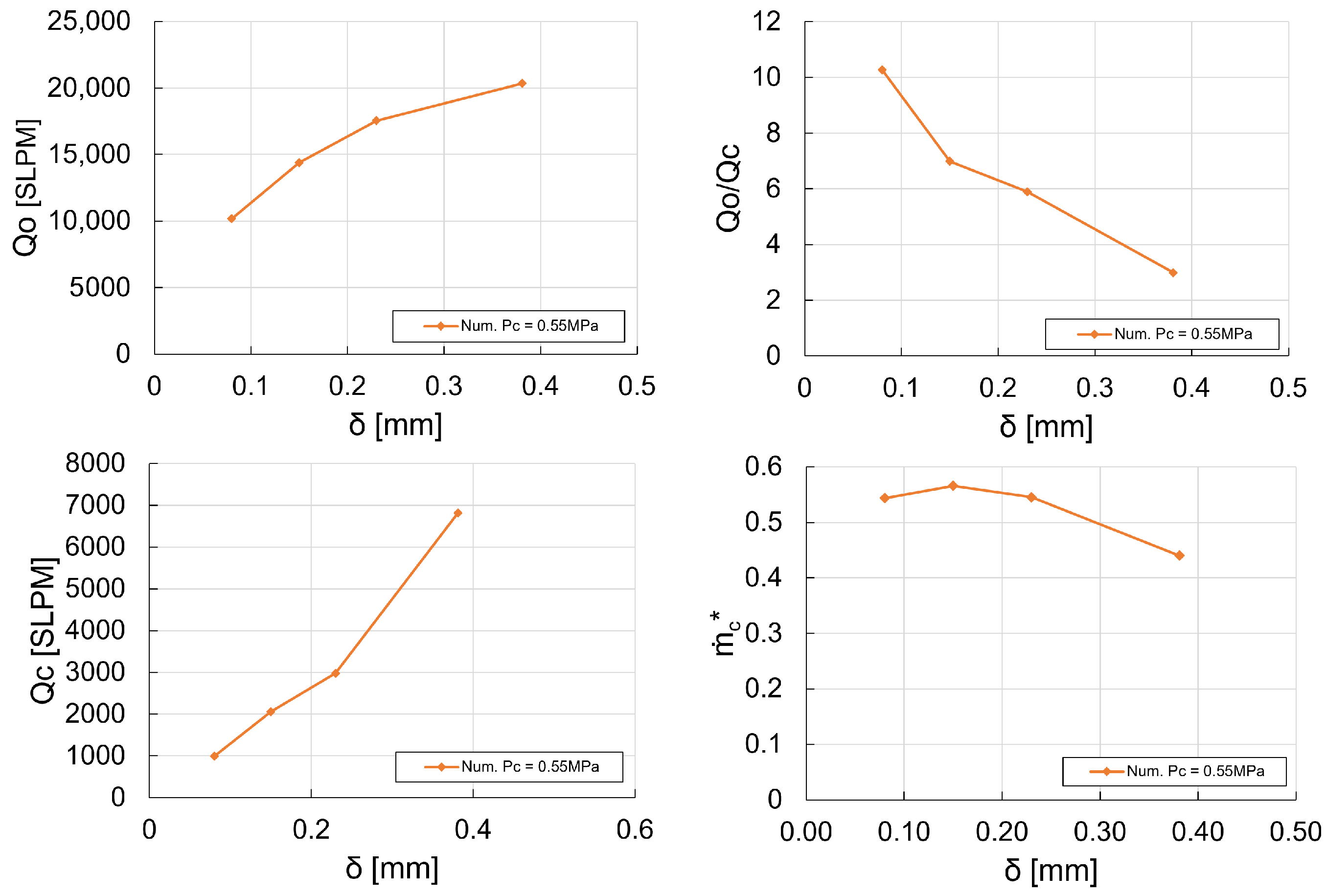
A wider range of values is explored for a fixed value of the primary flow upstream pressure, MPa. In Figure 26, the volumetric flow and the non-dimensional primary mass ratio are represented against the clearance distance , from mm to mm. The volumetric outflow and primary flow rate increase with the clearance gap. This leads to a decreasing trend in the volumetric flow ratio as the primary volumetric increases more drastically than the global outflow. Finally, the evolution of the non-dimensional mass flow indicates a saturation behavior for low values.
5.3.3. Geometry Sensitivity Study
For certain applications, it could be interesting to increase the amount of secondary mass flow. It can be magnified not only by increasing the high pressure value, , but also by scaling the entrainment area. Fixing the clearance gap, , and modifying other geometrical parameters allows us to explore the effects of scaling the air amplifier device.
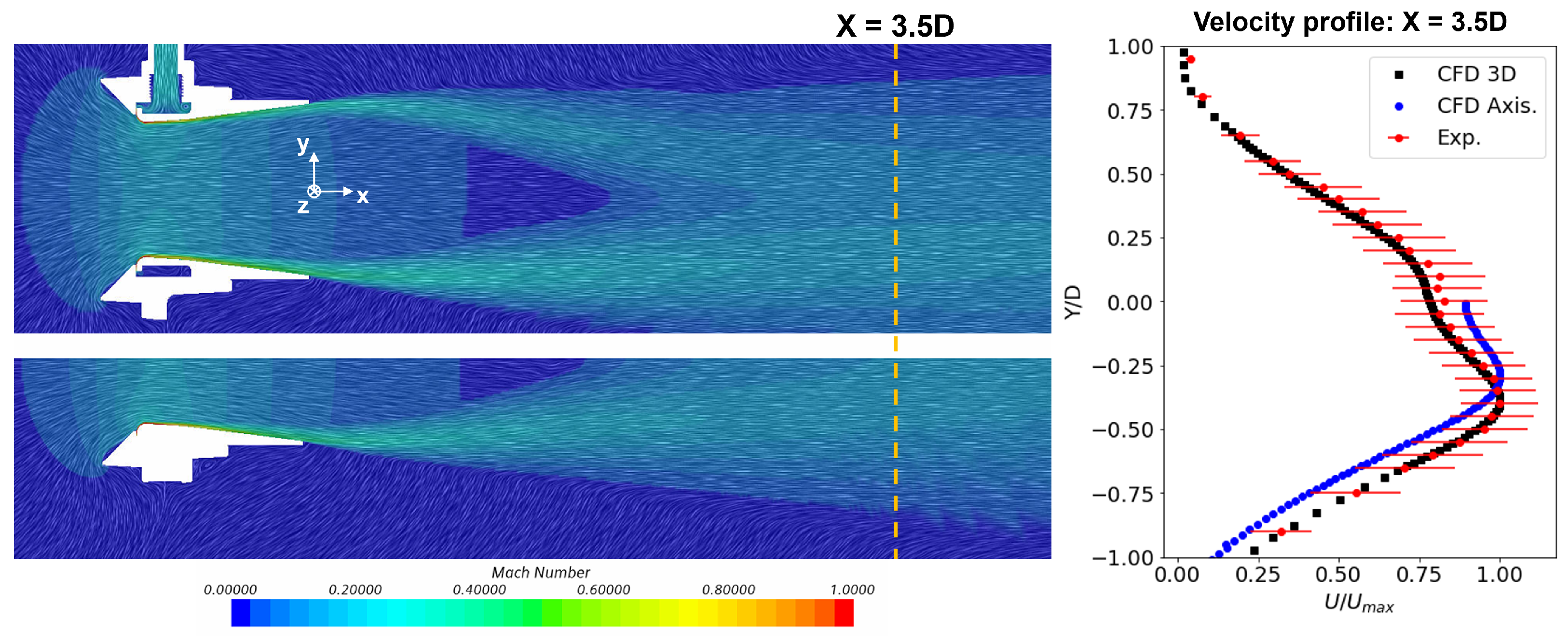
This study was conducted by employing axisymetric numerical simulations, as enunciated in Section 4.3. Comparing both the three-dimensional and the axisymmetric setup, the observed asymmetric behavior of the flow is lost in the axisymmetric simulations. However, the velocity profile recovered for the simplified model reproduces a similar trend and scaling compared to the 3D model, as shown in Figure 27 with MPa and mm. In Figure 27(left), Mach number contours are shown for a transversal slice ( m) of the 3D numerical simulation and compared with those obtained with the simplified axisymmetric one. Despite the loss in the slight asymmetric behavior, both show an excellent agreement. In Figure 27(right), velocity profiles measured at 3.5 diameters downstream from the air amplifier outlet are depicted, and experimental results are compared with numerical data for both the 3D and the simplified simulation. The variation in the results, which eliminate the non-symmetry, lands within the confidence interval defined by the standard deviation of the experimental measurements. To complete the analysis of different geometric parameters to evaluate the technical feasibility of the air amplifier to achieve a higher entrained flow, we therefore use the axisymmetric numerical setup to improve the computational cost.
Considering a fixed value of mm, three different values of the inlet total pressure, , and the amplifier inner diameter, , were considered. The set of studied cases is gathered in Table 3, with the first line being the original dimensions of the air amplifier. While increasing these geometrical or flow parameters leads to an increment in the injected and entrained mass flows, a saturation value of the amplification factor is eventually reached. For an scaled inner diameter, successive increments of the inlet total pressure do indeed produce larger entrained mass flows, but this does not translate into a better performance of the air amplifier. Comparing the nondimensional parameters in Table 3, however, may suggest a linear relationship between the aspect ratio defined by the internal diameter and the clearance gap, /, and the amplification factor, . Exploring larger values of / for different values offers a consistent behavior. A growing linear trend eventually reaches a clear maximum, with a later saturation of the amplification factor that rapidly decays. The maximum occurs for aspect ratio values between 1800 and 2000, independently of the gap size, which afterward shows a decreasing trend. These results are collected in Table 4. The air amplifier performance is based on its entrainment capability, which is related to the dragging effect of the pressure driven flow created by the annular jet. Thus, as the nozzle moves away from the axis of symmetry, the perturbation effects decay.
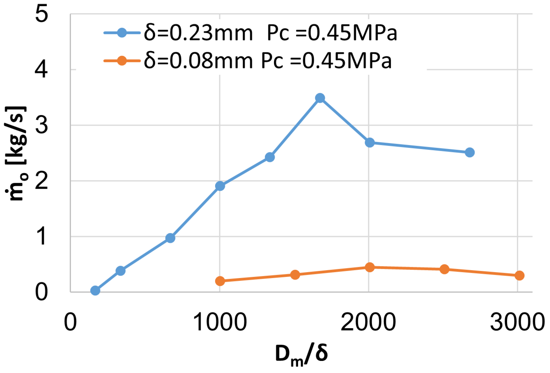
Interestingly, this relationship depends on the fixed gap size. Larger gaps present a maximum value of the total (injected+entrained) mass flow for aspect ratio values smaller than those observed for thinner gaps. This has been reflected in Figure 28, where gaps of mm and mm are compared. The observed behavior with a better performance of the smaller nozzle gap configurations (see Section 5.3.2) is consistent when the amplifier is scaled.
6. Conclusions
The performance evaluation of an industrial air amplifier involved comprehensive experimental and numerical analyses. The findings reveal that while both the injected and entrained mass flows increased linearly with the total pressure at the injection line, they exhibited different trends. Consequently, the amplification factor eventually reaches saturation, showing no further improvement when subjected to high input mass flows. Similarly, increasing the Coanda nozzle gap of the primary flow results in a linear growth in entrained mass flow, but these gains are penalized with a rapid decrease in efficiency. Thicker injection gaps result in lower amplification factors. This should be taken into consideration when the industrial application of the air amplifier requires displacement of large mass flows. These results are consistent in both modes of operation of the device, with these being either aspirating or blowing (depending on how the air amplifier is connected to an upstream or downstream piping system). However, the amplification factor observed during the experimental characterization showed higher values when working in the blowing mode, specially for larger nozzle gap sizes.
Scaling the air amplifier for greater total mass flows also led first to a saturating condition, followed by a decay in the air amplifier performance. By characterizing the aspect ratio defined by the internal diameter of the device and the clearance gap of the nozzle, how the total mass flows was observed, and the amplification factor reached a point beyond saturation, with a clear maximum, after which there was a significant decay in its values. This effect was also dependent on the nozzle gap size, with saturation occurring for higher values of the aspect ratio when thinner gaps were considered. An increase in volumetric mass flow was observed when the device was scaled, but it was more related to an increase in the outflow area rather than an increment on the flow velocity. As the flow entrainment is caused by the pressure drop caused by the flow displacement across the device, ultimately generated by the transfer of momentum from the annular jet towards the axis of symmetry, increasing the inner diameter would eventually produce a decay in the aforementioned effects.
These results underscore the sensitivity of air amplifiers to operating conditions and emphasizes the importance of tailoring the setup and sizing of the device to meet specific technical requirements. Considering the rapid decay in performance as the injected high-pressure mass flow increased, it is crucial to carefully consider the energy balance required for operating air amplifiers.
Author Contributions
A.M.-C. and M.C.-M. formulated the research plan and conceptualized the analyses, with support from S.M.-C. The numerical analyses were carried out by M.C.-M. and L.G. L.G. conducted a formal analysis of the numerical dataset, overseeing the employed methodology and managing resources, while M.C.-M. implemented and developed the validation, calculation, and interpretation of numerical results. The experimental studies were executed by A.M.-C. and S.M.-C., who equally contributed to the preparation and supervision of model manufacturing, conceptualization of the employed methodology, and data acquisition. M.C.-M. obtained the financial support for the project leading to this publication. A.M.-C. took charge of the original draft of the manuscript, with all authors participating in the final review and editing process. All authors have read and agreed to the published version of the manuscript.
Funding
This project has received funding from Airbus Operations Limited under the CDTI PTA (Programa Tecnológico Aeronáutico) 2021 program under grant agreement PTAG-20211002: Plan Tecnológico Aeronáutico ZERO (PTA_ZERO).
Institutional Review Board Statement
Not applicable.
Informed Consent Statement
Not applicable.
Data Availability Statement
The data presented in this study are available on request from the corresponding author.
Acknowledgments
The authors gratefully acknowledge the “Centro de Supercomputación y Visualización de Madrid” (CESVIMA) and Universidad Politécnica de Madrid for providing the computing resources on the Magerit Supercomputer.
Conflicts of Interest
The funders had no role in the design of the study; in the collection, analyses, or interpretation of data; in the writing of the manuscript; or in the decision to publish the results.
References
- Rubinetti, D.; Iranshahi, K.; Onwude, D.; Nicolaï, B.; Xie, L.; Defraeye, T. Electrohydrodynamic air amplifier for low-energy airflow generation—An experimental proof-of-concept. Front. Energy Effic. 2023, 1, 1140586. [Google Scholar] [CrossRef]
- Dai, H.K.; Huang, W.; Fu, L.; Lin, C.H.; Wei, D.; Dong, Z.; You, R.; Chen, C. Investigation of pressure drop in flexible ventilation ducts under different compression ratios and bending angles. Build. Simul. 2021, 14, 1251–1261. [Google Scholar] [CrossRef]
- Coanda, H. Propelling Device. US Patent 2,108,652, 5 February 1938. [Google Scholar]
- Morison, J.; Smith, D. Calculation of an Axisymmetric Turbulent Wall Jet over a Surface of Convex Curvature. Intl. J. Heat Fluid Flow 1984, 5, 139–148. [Google Scholar] [CrossRef]
- Smith, D.; Gilchrist, A. The Compressible Coanda Wall Jet—An Experimental Study of Jet Structure and Breakaway. Intl. J. Heat Fluid Flow 1987, 8, 156–164. [Google Scholar] [CrossRef]
- Gilchrist, A.; Smith, D. Compressible Coanda Wall Jet: Predictions of Jet Structures and Comparison with Experiment. Intl. J. Heat Fluid Flow 1988, 9, 99–107. [Google Scholar] [CrossRef]
- Smith, D.; Senior, P. The Effect of Base Steps and Axisymmetry on Supersonic Jets over Coanda Surfaces. Intl. J. Heat Fluid Flow 1994, 15, 291–298. [Google Scholar] [CrossRef]
- Kim, H.; Raghunathan, S.; Setoguchi, T.; Matsuo, S. Experimental and numerical studies of supersonic coanda wall jets. In Proceedings of the 38th Aerospace Sciences Meeting and Exhibit, Berlin, Germany, 14 September–9 October 2000; p. 814. [Google Scholar] [CrossRef]
- Ameri, M. An Experimental and Theoretical Study of Coanda Ejectors. Ph.D. Thesis, Case Western Reserve University, Cleveland, OH, USA, 1993. [Google Scholar]
- Wallace, J.; Choong, C. Fan Heater. US Patent D672,023 S, December 4, 2012. [Google Scholar]
- Rubinetti, D.; Iranshahi, K.; Onwude, D.I.; Xie, L.; Nicolaï, B.; Defraeye, T. An in-silico proof-of-concept of electrohydrodynamic air amplifier for low-energy airflow generation. J. Clean. Prod. 2023, 398, 136531. [Google Scholar] [CrossRef]
- Alimohammadi, S.; Persoons, T. A Novel Linear Air Amplifier Technology to Replace Rotary Fans in Data Center Server Rack Cooling. In Proceedings of the 26th International Workshop on Thermal Investigations of ICs and Systems (THERMINIC), Berlin, Germany, 14 September–9 October 2020; pp. 1–6. [Google Scholar] [CrossRef]
- Oude Essink, E.H.; Persoons, T.; Alimohammadi, S. Parametric Investigation of Inlet Pressure and Diffuser Angle Impact on Adjustable Air Amplifier Performance. In Proceedings of the 2022 28th International Workshop on Thermal Investigations of ICs and Systems (THERMINIC), Dublin, Ireland, 28–30 September 2022; pp. 1–6. [Google Scholar] [CrossRef]
- Mo, S.; Wang, P.; Gao, R.; Chen, S.; Li, S. CFD-Based Numerical Simulation on the Combined Spraying Dust Suppression Device. Atmosphere 2022, 13, 1543. [Google Scholar] [CrossRef]
- Carlini, M.; Mennuni, A.; Rotondo, M.; Morelli, S. Numerical Simulation of Innovative Air Capture Systems Based on Bladeless Technology with Coandă effect. J. Fluid Flow Heat Mass Transf. 2022, 9, 1–9. [Google Scholar] [CrossRef]
- Sang-Hoon, S.; Ran-Hui, K.; Sang-Min, K.; Nam-Hoon, L.; Jin-Kyu, P. Effect of landfill in-situ aeration with novel air amplifier: A case study. Environ. Eng. Res. 2023, 28, 230051. [Google Scholar] [CrossRef]
- Dixon, R.B.; Muddiman, D.C.; Hawkridge, A.M.; Fedorov, A. Probing the Mechanisms of an Air Amplifier Using a LTQ-FT-ICR-MS and Fluorescence Spectroscopy. J. Am. Soc. Mass Spectrom. 2007, 18, 1909–1913. [Google Scholar] [CrossRef] [PubMed]
- Robichaud, G.; Dixon, R.B.; Potturi, A.S.; Cassidy, D.; Edwards, J.R.; Sohn, A.; Dow, T.A.; Muddiman, D.C. Design, modeling, fabrication, and evaluation of the air amplifier for improved detection of biomolecules by electrospray ionization mass spectrometry. Int. J. Mass Spectrom. 2011, 300, 99–107. [Google Scholar] [CrossRef] [PubMed]
- Jurčíček, P.; Liu, L.; Zou, H. Numerical simulation of Monte Carlo ion transport at atmospheric pressure within improved air amplifier geometry. Int. J. Ion Mobil. Spectrom. 2014, 17, 157–166. [Google Scholar] [CrossRef]
- Kim, H.D.; Rajesh, G.; Setoguchi, T.; Matsuo, S. Optimization study of a Coanda ejector. J. Therm. Sci. 2006, 15, 331–336. [Google Scholar] [CrossRef]
- Lee, J.M.; Cho, M.Y.; Hong, C.K.; Yoon, S.M.; Kim, H.S.; Kim, Y.J. Effect of Coanda nozzle clearance on the flow characteristics of air amplifier. In Proceedings of the 2014 ISFMFE—6th International Symposium on Fluid Machinery and Fluid Engineering, Wuhan, China, 22 October 2014; pp. 1–6. [Google Scholar] [CrossRef]
- Oude Essink, E.H.; Persoons, T.; O’Brien, G.; Alimohammadi, S. Numerical Investigation of Adjustable Air Amplifiers as an Alternative to Fans in Data Centre Servers. In Proceedings of the 2022 21st IEEE Intersociety Conference on Thermal and Thermomechanical Phenomena in Electronic Systems (iTherm), San Diego, CA, USA, 1 May 2022–3 June 2022; pp. 1–6. [Google Scholar] [CrossRef]
- Lee, J.M.; Jo, Y.S.; Kim, S.M.; Kim, Y.J. Effect of Aspect Ratios on the Performance Characteristics of Air Amplifier. Volume 1A: Symposia, Part 2. In Proceedings of the Fluids Engineering Division Summer Meeting, Seoul, South Korea, 26–31 July 2015. [Google Scholar] [CrossRef]
- Exair Web Catalog 31 Air Amplifiers. 2022. Available online: https://www.pneuma.pl/wp-content/uploads/2017/08/AirAmplifiers.pdf (accessed on 5 January 2022).
- ISO 5167-3:2003; Medición del Caudal de Fluidos Mediante Dispositivos de Presión Diferencial Intercalados en Conductos en Carga de SeccióN Transversal Circular. AENOR: Madrid, Spain, 2003.
- Comte-Bellot, G. Hot-Wire Anemometry. Annu. Rev. Fluid Mech. 1976, 8, 209–231. [Google Scholar] [CrossRef]
- Menter, F. Zonal two equation k-ω turbulence models for aerodynamic flows. In Proceedings of the 23rd Fluid Dynamics, Plasmadynamics, and Lasers Conference, Orlando, FL, USA, 6–9 July 1993; p. 2906. [Google Scholar] [CrossRef]
- Shih, T.H.; Liou, W.W.; Shabbir, A.; Yang, Z.; Zhu, J. A new k-ε eddy viscosity model for high reynolds number turbulent flows. Comput. Fluids 1995, 24, 227–238. [Google Scholar] [CrossRef]
Figure 1.
Sketch of the EXAIR Super Air Amplifier 120024 operation (left) and static pressure contours on an operating condition (right).
Figure 1.
Sketch of the EXAIR Super Air Amplifier 120024 operation (left) and static pressure contours on an operating condition (right).

Figure 2.
Geometrical parameters air amplifier geometry (left) and detailed view of the compressed flow inner duct and the Coanda nozzle gap clearance (right).
Figure 2.
Geometrical parameters air amplifier geometry (left) and detailed view of the compressed flow inner duct and the Coanda nozzle gap clearance (right).

Figure 3.
Air tank (left) and details of its outflow pressure regulation control (right).

Figure 4.
Main dimensions of the Venturi tube (in mm).

Figure 5.
Assembly of the Venturi tube parts and methacrylate tube.

Figure 6.
Detail of the CNC milled Venturi tube constriction (left) and the air amplifier fitting (right).
Figure 6.
Detail of the CNC milled Venturi tube constriction (left) and the air amplifier fitting (right).

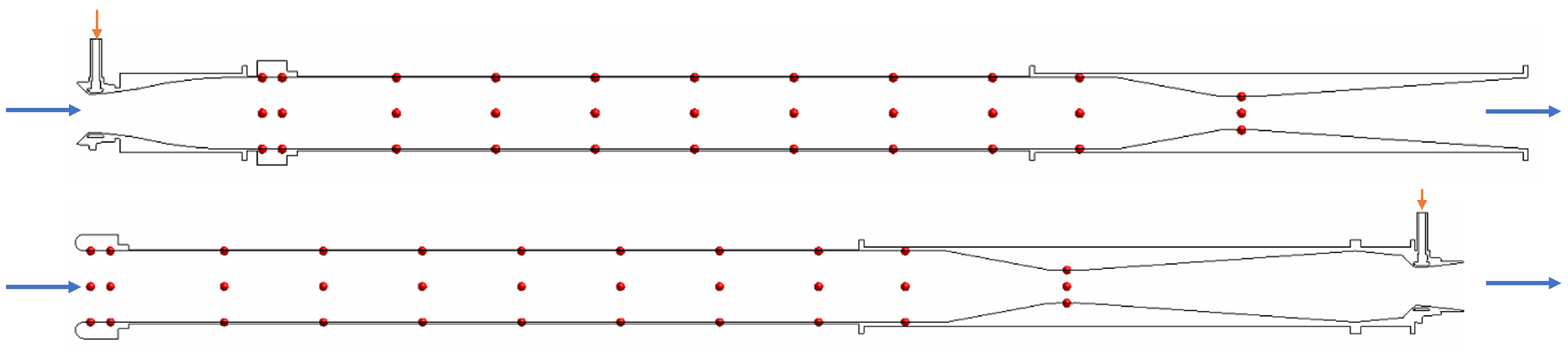
Figure 7.
Experimental configurations based on the air amplifier location with respect to the Venturi tube constriction. Blowing mode (upper image) and suction mode (lower image). The locations of the pressure taps are marked with red dots, and the blue arrow indicates the flow direction.
Figure 7.
Experimental configurations based on the air amplifier location with respect to the Venturi tube constriction. Blowing mode (upper image) and suction mode (lower image). The locations of the pressure taps are marked with red dots, and the blue arrow indicates the flow direction.

Figure 8.
Details of the pressure tap inserts inside the Venturi tube.

Figure 9.
Full experimental blowing setup for the mass flow measurement.

Figure 10.
Electronic pressure scanning module and pressure line array.

Figure 11.
Differential pressure transducers used on the Venturi tube constriction section.

Figure 12.
Hot wire measurement setup (left) and three-component probe close-up view (right).

Figure 13.
Sketch of the computational domain and boundary conditions considered for the isolated case.
Figure 13.
Sketch of the computational domain and boundary conditions considered for the isolated case.

Figure 14.
Three different levels of detail of the mesh at section m.

Figure 15.
Geometry comparison between 3D (left) and axisymmetric (right) model.

Figure 16.
Blowing mode. High-pressure line volumetric mass flow, ; entrained volumetric mass flow, ; and amplification factor , against the total pressure measured at the inlet of the air amplifier .
Figure 16.
Blowing mode. High-pressure line volumetric mass flow, ; entrained volumetric mass flow, ; and amplification factor , against the total pressure measured at the inlet of the air amplifier .

Figure 17.
Suction mode. High-pressure line volumetric mass flow, ; entrained volumetric mass flow, ; and amplification factor , against the total pressure measured at the inlet of the ESAA .
Figure 17.
Suction mode. High-pressure line volumetric mass flow, ; entrained volumetric mass flow, ; and amplification factor , against the total pressure measured at the inlet of the ESAA .

Figure 18.
Wake velocity profile at three downstream transversal sections (from left to right columns, , , and , respectively). Streamwise (u), crossed-vertical (v) and crossed-horizontal (w) velocities are plotted from numerical (■) and experimental () tests, including experimental standard deviation.

Figure 19.
Comparison of numerical and refined experimental velocity profiles at downstream section . Mean values of streamwise velocity are plotted from numerical (■) and experimental () tests. Red lines depict the standard deviation of the experimental data.
Figure 19.
Comparison of numerical and refined experimental velocity profiles at downstream section . Mean values of streamwise velocity are plotted from numerical (■) and experimental () tests. Red lines depict the standard deviation of the experimental data.

Figure 20.
Velocity magnitude streamlines at section m (top) and m (bottom).

Figure 21.
Line integral convolution colored by local Mach number values at sections m (left) and m (right).
Figure 21.
Line integral convolution colored by local Mach number values at sections m (left) and m (right).

Figure 22.
Mach number contours depicting supersonic regime across the injection gap and the Coanda profile. Flow data from simulations performed for MPa.
Figure 22.
Mach number contours depicting supersonic regime across the injection gap and the Coanda profile. Flow data from simulations performed for MPa.

Figure 23.
Primary volumetric flow (left) and non-dimensional mass flow (right) at different primary flow pressure . Gap clearance of mm.
Figure 23.
Primary volumetric flow (left) and non-dimensional mass flow (right) at different primary flow pressure . Gap clearance of mm.

Figure 24.
Mach number at different primary flow pressure when the clearance is mm.

Figure 25.
Variation in the outlet volumetric flow rate (top-left), outlet/primary flow rate ratio (top-right), primary volumetric flow rate (bottom-left), and non-dimensional mass flow (bottom-right) for different values of the clearance distance value .
Figure 25.
Variation in the outlet volumetric flow rate (top-left), outlet/primary flow rate ratio (top-right), primary volumetric flow rate (bottom-left), and non-dimensional mass flow (bottom-right) for different values of the clearance distance value .

Figure 26.
Variation in the outlet volumetric flow rate (top-left), outlet/primary flow rate ratio (top-right), primary volumetric flow rate (bottom-left), and non-dimensional mass flow (bottom-right) for different values of the clearance distance with MPa.
Figure 26.
Variation in the outlet volumetric flow rate (top-left), outlet/primary flow rate ratio (top-right), primary volumetric flow rate (bottom-left), and non-dimensional mass flow (bottom-right) for different values of the clearance distance with MPa.

Figure 27.
Comparison of the numerical results obtained for a 3D and an axisymmetric simulation with MPa and mm. Contours of flow Mach number are shown in the left image for both cases, together with streamwise velocity distributions in the right image. The experimental data include the standard deviation of the measured values.

Figure 28.
Variation in the total (injected+entrained) mass flow, , with the relation between the inlet diameter and the gap width, , for two different gap values at MPa.
Figure 28.
Variation in the total (injected+entrained) mass flow, , with the relation between the inlet diameter and the gap width, , for two different gap values at MPa.


Table 1.
Dimensions of the air amplifier.
| Dimension [mm] | |
|---|---|
| 9.525 | |
| 121.3 | |
| 97.42 | |
| 76.50 | |
| 86.00 | |
| [0.08, 0.15, 0.23, 0.38] |
Table 2.
Grid convergence process and volumetric flow ratio relative error.
| Grid | Reference Grid Size [mm] | Number of Elements | [%] | |
|---|---|---|---|---|
| 5 | 622,536 | 21.22 | - | |
| 2.5 | 2,784,133 | 24.06 | 11.8 | |
| 1.25 | 9,025,234 | 23.62 | 1.9 | |
| 0.625 | 15,103,121 | 23.90 | 1.2 |
Table 3.
Results of the air amplifier geometry scaling.
| [MPa] | [mm] | [m] | / | [kg/s] | [kg/s] | [SLPM] | [SLPM] | |
|---|---|---|---|---|---|---|---|---|
| 0.45 | 0.23 | 0.0765 | 334 | 0.05 | 0.38 | 2380 | 18,142 | 7.6 |
| 0.45 | 0.23 | 0.3060 | 1338 | 0.17 | 2.42 | 8275 | 114,205 | 13.8 |
| 0.45 | 0.23 | 0.3825 | 1673 | 0.22 | 3.49 | 10,343 | 164,024 | 15.8 |
| 0.60 | 0.23 | 0.3825 | 1673 | 0.28 | 4.68 | 13,247 | 220,177 | 16.6 |
| 0.80 | 0.23 | 0.3825 | 1673 | 0.42 | 5.68 | 16,996 | 267,168 | 15.7 |
Table 4.
Variation in the total (injected+entrained) mass flow, , with the relation between the inlet diameter and the gap width, , for two different gap values and MPa.
Table 4.
Variation in the total (injected+entrained) mass flow, , with the relation between the inlet diameter and the gap width, , for two different gap values and MPa.
| [mm] | [m] | / | [kg/s] | [kg/s] | [SLPM] | [SLPM] | |
|---|---|---|---|---|---|---|---|
| 0.23 | 0.0383 | 167 | 0.026 | 0.031 | 1219 | 1478 | 1.2 |
| 0.0765 | 334 | 0.051 | 0.386 | 2381 | 18,142 | 7.6 | |
| 0.1530 | 669 | 0.097 | 0.974 | 4568 | 45,819 | 10.0 | |
| 0.2295 | 1003 | 0.148 | 1.910 | 6963 | 89,853 | 12.9 | |
| 0.3060 | 1338 | 0.176 | 2.428 | 8275 | 114,205 | 13.8 | |
| 0.3825 | 1673 | 0.220 | 3.487 | 10,344 | 164,025 | 15.9 | |
| 0.4590 | 2007 | 0.253 | 2.687 | 11,916 | 126,403 | 10.6 | |
| 0.6120 | 2677 | 0.314 | 2.513 | 14,758 | 118,216 | 8.0 | |
| 0.08 | 0.0765 | 1004 | 0.015 | 0.199 | 693 | 9368 | 13.5 |
| 0.1148 | 1506 | 0.021 | 0.313 | 981 | 14,729 | 15.0 | |
| 0.1530 | 2008 | 0.026 | 0.446 | 1240 | 20,986 | 16.9 | |
| 0.1913 | 2510 | 0.031 | 0.413 | 1481 | 19,434 | 13.1 | |
| 0.2295 | 3012 | 0.033 | 0.301 | 1557 | 14,159 | 9.1 |
Disclaimer/Publisher’s Note: The statements, opinions and data contained in all publications are solely those of the individual author(s) and contributor(s) and not of MDPI and/or the editor(s). MDPI and/or the editor(s) disclaim responsibility for any injury to people or property resulting from any ideas, methods, instructions or products referred to in the content. |
© 2024 by the authors. Licensee MDPI, Basel, Switzerland. This article is an open access article distributed under the terms and conditions of the Creative Commons Attribution (CC BY) license (https://creativecommons.org/licenses/by/4.0/).
Share and Cite
MDPI and ACS Style
Chávez-Módena, M.; Martinez-Cava, A.; Marín-Coca, S.; González, L. Numerical and Experimental Characterization of a Coanda-Type Industrial Air Amplifier. Appl. Sci. 2024, 14, 1524. https://doi.org/10.3390/app14041524
AMA Style
Chávez-Módena M, Martinez-Cava A, Marín-Coca S, González L. Numerical and Experimental Characterization of a Coanda-Type Industrial Air Amplifier. Applied Sciences. 2024; 14(4):1524. https://doi.org/10.3390/app14041524
Chicago/Turabian StyleChávez-Módena, Miguel, Alejandro Martinez-Cava, Sergio Marín-Coca, and Leo González. 2024. "Numerical and Experimental Characterization of a Coanda-Type Industrial Air Amplifier" Applied Sciences 14, no. 4: 1524. https://doi.org/10.3390/app14041524
Note that from the first issue of 2016, this journal uses article numbers instead of page numbers. See further details here.