
New Empirical Laws in Geosciences: A Successful Proposal
by
 , , , and
Jesús Díaz-Curiel
1,* ,
,
Bárbara Biosca
1,
Lucía Arévalo-Lomas
1,
David Paredes-Palacios
2 and
María Jesús Miguel
3 1
Department of Energy and Fuels, School of Mines and Energy, Universidad Politécnica de Madrid, C/Ríos Rosas 21, 28003 Madrid, Spain
2
Department of Geological and Mining Engineering, School of Mines and Energy, Universidad Politécnica de Madrid, C/Ríos Rosas 21, 28003 Madrid, Spain
3
Spanish Ministry of Science and Innovation, Paseo de la Castellana 162, 28046 Madrid, Spain
*
Author to whom correspondence should be addressed.
Appl. Sci. 2023, 13(18), 10321; https://doi.org/10.3390/app131810321
Submission received: 14 July 2023
/
Revised: 8 September 2023
/
Accepted: 12 September 2023
/
Published: 14 September 2023
Abstract
:The importance of empirical versus theoretical laws is a controversial issue in many scientific fields, the latter being generally accepted and the relevance of which is not discussed here. As in other areas, there are well-known theoretical and empirical formulas in geosciences that do not adequately represent the reality of a given phenomenon. Quantitative comparison of geophysical and petrophysical results with data from the other multiple fields that comprise the geosciences compels a high exigency to avoid discontinuities in existing relationships. However, the proposal of new empirical laws that more accurately reflect a given phenomenon is often considered insufficient to contradict existing formulas. The aim of this work is to defend the development of new empirical laws by showing that they constitute a true model of analysed behaviour if certain criteria are followed. This defence is especially needed when non-linearisable functions are required to fit the empirical data. To achieve this aim, this study shows the established algebraic function as a function of a single variable, whose main advantage is its application to phenomena of a geological nature that show two differentiated behaviours as the variable x is increased. A series of five examples of different phenomena related to geosciences is selected to demonstrate the level of accuracy that new empirical laws can reach in contrast to the widely accepted historical relationships.
1. Introduction
Contrary to theoretical laws, which are generally accepted, the new empirical laws in geosciences that disagree with existing concepts and formulas often face more objections to being accepted by the research community, thus reflecting a certain reluctance to accept these types of laws. In the authors’ experience, concerns about the new empirical relationships have not arisen due to the omission of any relevant variable suggesting a limited understanding of the phenomenon under study but expressly due to their discordance with the existing ones. The main criticism of new empirical laws is often dependent on the existence of previous relationships whose results differ from those obtained using the presented laws. Further criticism arises when the new empirical law is not presented in the form of a well-known function such as linear, power, or exponential (polynomial functions are not included because of the difficulty of assigning them a physical sense), which is seemingly interpreted as if something is hidden or mysterious. New empirical laws often encounter dogmatic criticism, as no arguments about the erroneous basis for the development of the new formula are presented, and the goodness of obtained fit or high correlation between the proposed function and empirical data are frequently ignored in the peer review process, even when superior to those of existing laws.
Establishing a simple algebraic function that is shown to encompass several very different phenomena in geological media leads to milestones with respect to the functions conventionally used to fit them. Phenomena in which the gradient of a variable y varies gradually with the independent variable x generally tries to fit power or exponential functions (both linearisable) unless prior knowledge is available to facilitate the use of a specific function. However, there are many cases in practice in which the empirical data do not adequately fit these types of functions but correspond to two different behaviours dependent on the variation of the independent variable. This study presents a new type of single variable function, named the function of double asymptote, which allows the acceptance of new empirical laws, unlike other more complex processes such as the one shown in Godoy et al. [1], and those showing a single asymptote are usually studied using the empirical Hurst’s law [2]. A function of double asymptote of a single variable is one that presents an infinite approximation to a straight line (horizontal, vertical, or oblique), i.e., an asymptotic behaviour, at two different values, and these functions have been called y2A(x). If fitting a comprehensive data series to a function of double asymptote y2A(x) is substantially better, it implies that the phenomenon under analysis responds to two different behaviours. The examples presented here show how an existing expression may not be useful for covering a geological reality.
The aim of this work is to demonstrate that it is, today, possible and necessary to develop mathematical expressions that faithfully represent some of the many phenomena that occur in different fields of geosciences. If a new relationship is obtained from empirical data and meets certain requirements (stated below), this law should be accepted despite its results contrasting with those of previous models. The need to develop these new empirical laws arises because the existing relationships are restricted due to poor fit, continuity problems, lack of meaning beyond the analysed range, or other deficiencies.
This study is focused on the development of empirical laws as a possible analytical (mathematical) solution to a given phenomenon in geosciences. Defending the possibilities of empirical laws does not imply being against theoretical laws, nor is the intention to evaluate the bases, tools, methods, and theoretical developments. In this study, it is considered that analytical solutions in general, and empirical laws in particular, should aim to avoid discontinuities, except when analysing physically discontinuous phenomena. Hence, added to the above objective is the proposition that the new empirical laws should continuously reflect the behaviour of natural media involving two distinct processes that do not conform to conventional mathematical expressions of fit. One of the reasons for defending empirical laws in complex phenomena lies in the fact that the step from the infinitesimal theoretical formulation to the behaviour at a macroscopic scale (characteristic in geosciences) involves the statistical generalisation of many variables, which does not always conclude in an analytical expression.
This work affirms that it is still necessary to investigate certain phenomena in geosciences in order to obtain new empirical laws that represent their behaviour. The y2A(x) functions presented in this study demonstrate their usefulness in obtaining empirical laws that accurately fit the empirical data. The applied character of the presented examples supports the validity and use of empirical laws that allow a more realistic reflection of the main characteristics of the phenomena analysed.
This work begins by framing the diatribe between empirical and theoretical laws, the diversity of physical aspects that make up the geosciences, and the difference between more descriptive (e.g., case studies) and methodological advances in this field, although these aspects may also be found in other scientific fields. Some criteria are provided for outlining function fitting to empirical data. The process by which the most appropriate function is selected is not presented for each case because this search requires a tremendously broad catalogue of diverse functions. The study then focuses on showing the established function type, named functions of double asymptote y2A(x), specifically designed to model natural phenomena involving two different behaviours depending on changes in a single variable x. Some empirical relationships developed and published by authors in recent years in sufficiently differentiated fields: petrophysics [3], fluid flow in porous media [4], geotechnics [5], nuclear magnetic resonance [6], and spread of radioactive emissions [7] are presented as examples. In the discussion, some possible generic objections against the development of new empirical relationships are presented.
2. Materials and Methods
2.1. Theoretical Laws Versus Empirical Laws
Scientific laws can be described as reasonings that determine a univocal relationship between different parameters or properties of an analysed medium or process, and they can generally be represented by a mathematical expression. Theoretical laws are generally considered to be those that enunciate a certain principle that relates to these properties or are based on other general laws and accepted principles. Conversely, empirical laws are based on empirical data, and the criterion for generating the function that relates the analysed variables simply involves data fitting to a certain function. Nevertheless, an empirical law can facilitate the subsequent development of a theoretical law.
The qualification of “laws” given to these relationships applies to phenomena that involve a great generality, e.g., Newton’s second law, and those whose impact is limited to a specific field, e.g., Darcy’s law [8] for water flow in semi-permeable porous media and Archie’s first law [9] in petrophysics. A conventional way for accordingly differentiating laws is to qualify the former as universal laws. The labelling of laws is generally reserved for equations in which an analysed relationship between different parameters is established for the first time. Although once established, these relationships typically undergo improvements of their applied coefficients; they must not be considered as new laws. In other cases, certain definitions may change the final expression of an established law; for example, Poiseuille’s law [10] was determined before the definition of viscosity.
Interestingly, relationships of great interest are not always formalised as laws. As an example, starting from empirical values, Sundberg [11] established that the ratio between the resistivities of a solid porous medium ρ0 and fluid that fills its pores ρW presents a constant value, which was initially called the resistivity factor and later the formation factor F. Archie [9] later empirically determined that F = 1/Øm, where Ø is the porosity of the analysed medium and m is its characteristic parameter, which would eventually be referred to as the cementation exponent. Apart from the confusion involved in the naming of this exponent, because it does not solely depend on the presence of cement in the analysed medium, this relationship is known in petrophysics as Archie’s first law. However, the establishment of the formation factor was not attributed to the character of a law, even though this factor is an intrinsic parameter of geological media and provides considerably greater characterisation.
The application range of a given relationship must also be considered to qualify an obtained law. Although the qualification as a law for empirical laws is relative—and somewhat pretentious—compared with universal laws, it can be said that a relationship is considered a law when it is applicable to a large number of cases in a given field. For example, although water is considered a reference fluid and NaCl is a characteristic ionic bonding compound, the relationship between conductivity (σ) in μS/cm and concentration (CC) in g/cm3 of a NaCl solution in water, given by CC(NaCl) = σ2/[1500·(σ + 500)] [12] should not be considered an empirical law because this relationship does not hold for other salts.
An objection that is often posed to new empirical laws is their lack of theoretical basis, even though some empirical laws have achieved recognition similar to that of theoretical laws. The most recognised example is the law of universal gravitation. However, a fact that offsets the importance of empirical laws is that some of the most recognised theoretical equations have arisen from one or more empirical laws, as in the case of Maxwell’s equations for electromagnetic fields, which combines the previous laws of Ampere, Gauss, and Faraday. A similar phenomenon occurs with the equation of transport in fluid media, which combines the laws of Newton on viscosity (1687), Darcy (1856), and Fick (1955), among others, although the consideration of the different included phenomena involves the addition of empirical relationships that regulate each phenomenon. In some cases, the requirement of a theoretical basis has led to an initial error in the application of previous laws, generally by considering the applicability of the model they represent. One example is the case in which the equations of flow in straight capillaries are considered to govern flow in porous geological media, which have been shown to be inappropriate for isotropic homogeneous media [13].
The degree of objection to new empirical laws and the requirement of theoretical justification depends, to a large extent, on the specific characteristics of each scientific field. Some particularities within the geosciences are therefore discussed in the following section.
2.2. Knowledge-Based Approaches in Geosciences
Research in geoscience, as in other scientific fields, involves two types of contributions to knowledge, in which case studies are differentiated from those that develop new methods or whose results are generalisable. The first type of contribution presents specific data of a study area that were not previously known (e.g., cartography, basin descriptions, and seismic sections). The other type of contribution presents a novel technique for obtaining data, new algorithms for data processing or interpretation, or new reasoning on the obtained data that explains why the data behave in an observed manner. Among the latter, there are investigations in which principles and rules that govern the analysed phenomenon, typically constituting theoretical laws, are deduced based on theoretical reasoning. There are also investigations in which relationships are developed to estimate a certain property of an analysed process as a function of some other properties based on the observed data, possessing a degree of predictive capacity, and these are used to establish empirical laws.
The particularities presented in this work on empirical laws refer to studies in which these rules are materialised in the form of a mathematical relationship between analysed variables or parameters, such as density as a function of depth or porosity as a function of grain size distribution. The described difference is independent of its greater or lesser significance. There have thus been great contributions to geological knowledge that did not require a mathematical relationship, such as the explanation of continental movement via plate tectonics.
As in many scientific fields, another widespread way to achieve the aforementioned predictive nature in geoscience involves mathematical modelling using finite element or finite difference methods, the main limitation of which is that they must be considered for each specific case. The theoretical starting point is sometimes limited when applying these techniques; for example, in the Monte Carlo modelling of radioactive spreading in subsoil, the effect of accumulation is not considered [7]. The same occurs in the modelling of flow in porous media when considering a tortuosity expression that does not reflect the real tortuosity [13].
2.3. Criteria for the Development of Empirical Laws
For a given phenomenon, there may be several functions with similar fits to the empirical data. The selection of a fitting function thus becomes the key that determines the quality of the obtained law in many cases. Functions that can be used to generate empirical relationships range from simple proportionality to progressively more complex expressions (e.g., explicit relationships of the friction factor in rough pipes to fit the non-analytical-resoluble Colebrook equation [14] for rough pipes). In this sense, although there is no universal principle according to which aspect of nature must be governed by simple relationships, the search for empirical relationships that reflect natural behaviour must have this aim, at least in principle.
The simplest functions are linear or linearisable functions (exponential and logarithmic) [15,16,17,18], which are often used owing to the ease by which their coefficients are obtained, and the use of polynomial functions is also common [19,20]. Nevertheless, it must be noted that a possible physical meaning is difficult to assign to polynomials with an order higher than 2, except for those that correspond to the powers of binomials. The presentation of an empirical law of this type is generally not disputed because of its inclusion in well-known calculation codes (e.g., MS Excel©, Version 1808, Office 2019), even though these functions are often meaningless beyond the applied range. In contrast, in the authors’ experience, strong reluctance is common when a non-typical function is used, even if the resulting goodness of fit to the empirical data is higher using the new empirical law or if an existing relationship is not contradicted.
One consideration that must be faced before searching for a mathematical relationship that reflects a given process is the continuities and discontinuities that may exist in that process. Although the aesthetics of continuity is undeniable, certain discontinuous properties are common in natural media. A characteristic example is the phase transitions of water from solid to liquid and liquid to gas. Another not-so-well-known example is the flow regime transition of water between laminar and turbulent flow.
Some of the empirical relationships presented in this study only aimed to achieve the best fit to the empirical data without presenting, at first glance, an explanatory sense of the phenomenon. Example 4, shown below, is one such case that presents a new permeability relationship as a function of porosity in granular media and involves multiple factors. The developed law explains what actually occurs in nature rather than investigating how each involved variable affects that relationship. However, the obtained empirical law can facilitate the further development of a theoretical law.
A key aspect of the development of a new empirical law must be the validation of its results with empirical data. However, paradoxical cases are found in the literature. For example, the Kozeny equation [21] for estimating intrinsic permeability as a function of average grain size in porous media was developed, according to its author, for granular media with grains of the same size. However, it has been used as a validation of later models applied to media with different grain sizes. It is known that if the grain size distribution widens, the permeability decreases. In Díaz-Curiel et al. [22], a modification of this equation includes the grain size gradation coefficient, validated with the most recognised empirical data. The authors do not know how to explain the validation of the multitude of subsequent publications in which new equations were developed to estimate the permeability of media with different grain sizes and in which the Kozeny equation was used to validate their results.
Another example would be the equation established by Kleinberg and Horsfield [23] to describe the total nuclear magnetic resonance curve as a function of the three relaxation mechanisms (bulk B, surface S, and diffusion D) in all the pores of a granular medium. Although all the studies on this process agree that they are processes that occur in parallel, this equation proposed the analytical solution of this curve as the integral of the product of the exponentials corresponding to the three mechanisms. In Díaz-Curiel et al. [24], it was shown that this approach was incorrect because, among other reasons, it is contrary to the inverse Laplace decomposition with which the total resonance curve is solved according to all studies on this process (except that of the aforementioned equation and subsequent publications). This equation leads to the inference that the relaxation times fulfil the relation 1/T = 1/TB + 1/TS + 1/TD. The permeability values obtained using the last relation are very different from those obtained with the inverse Laplace decomposition analysis. Likewise, we do not know how to explain the empirical validations shown in the many publications in which it is used.
2.3.1. Limitations When Establishing Empirical Laws
The correct development of an empirical law must involve a physical sense of the established functional dependence, indicating which parameter depends on the rest of the variables. The fact that a function h(g) can be expressed in the form g(h) does not indicate that the latter reflects the dependence that occurs in nature. For example, the relation of fluid viscosity to its temperature does not imply that temperature depends on viscosity. Similarly, with respect to a fluid flowing through the pores of a porous medium, the fact that the cation exchange capacity (CEC) of the grains depends on the medium permeability does not imply that permeability depends on the CEC.
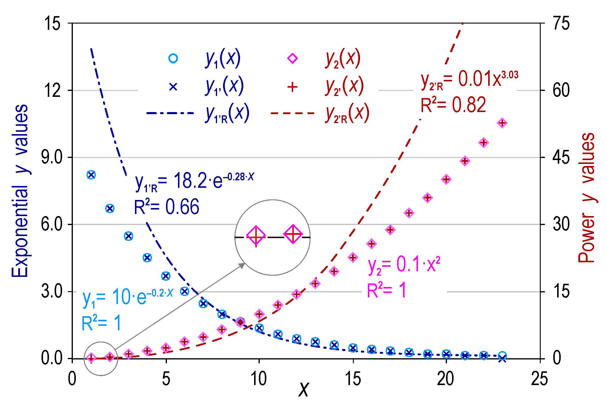
One of the empirical law limitations is the possibility of using different functions that reach a similar degree of deviation with respect to the empirical data. In this process, it should be considered that the use of goodness-of-fit indicators to evaluate a relationship to a set of empirical data (e.g., correlation coefficient, mean deviation, R2) may have limitations. For example, the least squares criterion to determine the fit coefficients of a linearisable function to a set of data, in which the variable x involves both very high and very low values, can provide fit coefficients that constitute a function that greatly deviates from the data if there is a significant disparity in one of the lowest values. To show this effect, consider two series of 23 data points, y1(x) = 10·exp(−0.2·x), and y2(x) = 0.1·x2 with (x = 1, …, 23), and two other series y1’(x) and y2’(x) with the same values except for an anomalous point of the lowest y values, for example, y1’(23) = 0.0001 (or another very close to zero) instead of 0.1 and y2’(1) = 0.0001 instead of 0.1. Figure 1 shows that the fitting functions y1’R(x) and y2’R(x) obtained using least squares to the y1’(x) and y2’(x) series substantially differ from y1(x) and y2(x).
The evaluation criteria for the goodness-of-fit relationship, which accounts for the number of measurements (e.g., the use of deviation σn−1 versus the standard deviation), should not be ignored. The indicator used in error minimisation processes should also be considered for cases involving a single variable or multiple variables by solving the Jacobian matrix, which is formed by the partial derivatives of the results with respect to the variables. Linear convergence that involves the absolute value of the difference can thus lead to different results than those obtained using a curved convergence, which involves the conventional least squares criterion (i.e., the root of the squared differences).
In a similar sense, the use of scales of a differentiated range (i.e., choice of axes) for parameters is not only a question of graphic representation but that the goodness of fit obtained using different criteria (e.g., regression coefficient R2) can lead to inaccurate results. For example, the relation between Young’s modulus of the ground ES and dynamic modulus ED (i.e., obtained from seismic propagation velocities) presents strong dispersion, which is seemingly eliminated if ES/ED is plotted against ED in a logarithmic scale.
Furthermore, there are other procedures that the authors consider to be inappropriate for determining empirical laws. For example, the result of multiplying or dividing an existing relationship by a factor does not strictly result in the establishment of a new law but rather a modification of the previous law. In other cases, it is used as an incorrect criterion that the new relationship is dimensionally consistent with a previous one (note that it is not a classical procedure of dimensional analysis).
2.3.2. Process for Obtaining Formulas
The first step to obtaining a certain empirical law is to analyse the geometry of the trends shown by the empirical data, for example, by paying attention to the number of curvatures, whether they show an increasing or decreasing trend, and whether they show asymptotic trends when the variable approaches lower or upper limit values or both. The logic of behaviour must be included in this process. For example, it is reasonable to consider that the porosity of a granular medium involving equidimensional grains is higher than that of a medium involving heterogeneous grain sizes, which can fill the remaining pores between those of a larger size, independently of whether this is confirmed by the empirical results.
After analysing the empirical data characteristics, a function that shows a similar aspect must be chosen. For non-harmonic behaviour, this step requires some knowledge on simple algebraic expressions. In this sense, the use of the trial-and-error method to select an initial ratio function should not be ruled out. Once a function is chosen, which should preferably contain few coefficients, the optimal value of these coefficients will be chosen to achieve the best fit to the empirical data, in which minimum deviation (i.e., adopting coefficients that minimise the difference between the fit function and empirical data) is an important criterion. This process can be performed using known codes, such as the MS Excel© solver function.
Although the individual steps to reach each formula are not shown in the different examples of empirical laws presented here, a common subsequent process has been searching secondary relationships for the coefficients of that first formula. For example, after analysing the trend of the empirical viscosity data of some silty-clay muds as a function of temperature (T), an ordinate determined at T ≥ 0 °C and an asymptotic decrease when T→100 °C was observed; thus, the most relevant function appears to be a decreasing exponential η(T) = a·exp(−b·T), where a and b are fitting coefficients. However, an adequate fit to the data cannot be achieved using any set of coefficients despite obtaining an acceptable regression coefficient (R2 = 0.93). Applying logarithms, it can be seen that the dependence of the data on temperature, with the exception of the constant value ln(a), shows that a power function explains the observed behaviour better. The chosen relationship for which the minimum deviation coefficients are calculated is η(T) = n1·exp(−n2·Tn3). An empirical relationship that more adequately describes that dependence (R2 = 0.99) is thus given as η(T) = 1.8·exp(−0.044·T0.85) by Díaz-Curiel [25]. However, this relationship cannot be considered a law, despite its usefulness in determining the changes in mud viscosity with temperature in water and oil wells, because the analysed fluid has somewhat specific characteristics.
2.4. A Fruitful Type of Double-Asymptotic Functions
The main reason for elaborating a new empirical relationship is the lack of a previous theoretical basis for presupposing the dependence of a parameter y on the values of an independent variable x. In some cases, the choice of function type has a theoretical explanation, such as exponential functions that solve the proportionality y ∝ x at differential level dy/dx = kC·y, which is the basis of many natural phenomena, where kC is a constant characteristic of the analysed phenomenon. However, in other phenomena that seem to show similar behaviour (e.g., growth attenuation in many living organisms), the empirical data do not properly fit exponential functions. In such cases, the choice of a function type only involves the generalised knowledge of certain simple functions. Thus, in addition to linear behaviour, cases in which the gradient of y varies gradually with x are generally applied to attempt to fit power or exponential (linearisable) functions. However, there are many cases in practice in which the empirical data do not adequately fit these types of functions. This study, therefore, considers it valuable to present a new type of simple function suitable for the acceptance of new empirical laws, as briefly stated in the introduction.
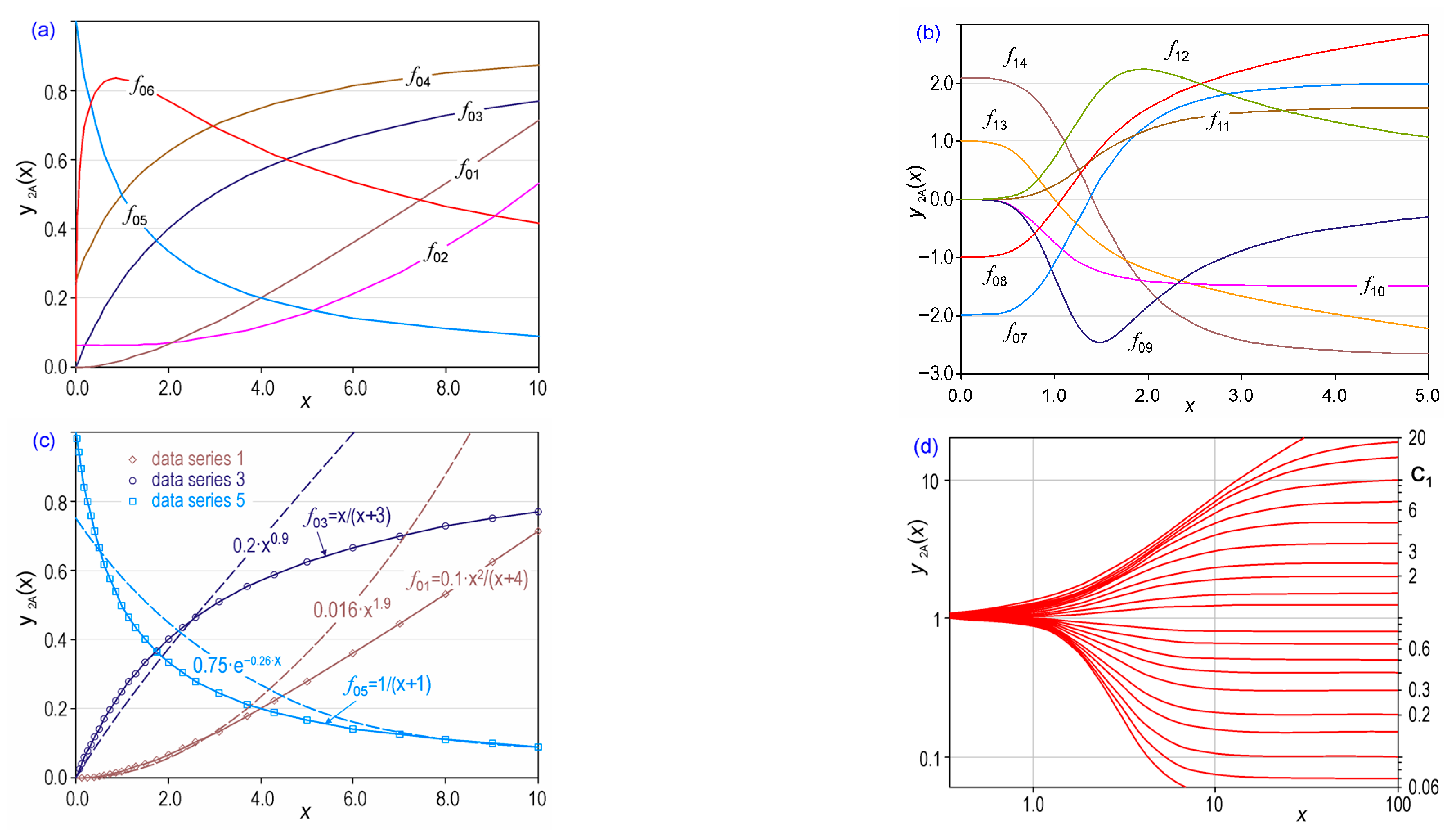
Among the many possible functions to choose from, a type of algebraic relationship defined for positive values of x is presented, which in this study are called functions of double asymptote y2A(x) because they exhibit asymptotic behaviour when the x values tend to 0 or infinity. The general form of these functions is:
Figure 2c shows that some curves with apparently exponential or power aspects clearly better fit to a function y2A(x), which reflect a variation of a determined gradient up to a given value of x and a different later gradient. Thus, despite obtaining high R2 values, the data series of function f01 do not fit a power function with a power greater than 1 (y = 0.016·x1.9, R2 = 0.99), those of function f03 do not fit a power function with a power less than 1 (y = 0.2·x0.9, R2 = 0.99), and those of function f05 do not fit an exponential function (y = 0.75·e0.26·x, R2 = 0.90).
Different asymptotic values can be obtained using different combinations of coefficients. Figure 2b shows some cases in which the two asymptotes are horizontal. It is also possible to obtain different asymptotic behaviours, such as from positive to horizontal, from horizontal to positive, and from negative to horizontal (Figure 2a). Furthermore, it is possible to fit x values with wide variation ranges, different curvatures (concave/convex), or where the inflexion point occurs at very different x values by varying the coefficients on these functions of double horizontal asymptote y2A(x). Even within this subtype, a suitable fit for different data sets can be achieved by varying the coefficients of the function. Figure 2d shows an example of the different behaviours captured by the function y2A(x) when all of the exponents are equal and c2 = c3; thus, the asymptotes on the left and right are y = 1 and y = c1, respectively.
The fit to a function y2A(x) is interesting because it may lead to a more theoretical law in the sense that it models an analysed parameter in a more diverse way than that corresponding to a single dependence, with this analysis and the subsequent one not being a purely theoretical development. This implies that if the fit to a function of double asymptote y2A(x) is substantially better than when using a power asymptote, the analysed phenomenon responds to two different behaviours, starting from the value of x at which the transition occurs (see examples 1 and 5); or if the two asymptotes have opposite directions, the analysed behaviour is also physically opposite (see example 4).
We should point out that the number of degrees of freedom of the function y2A(x) depends on the geometry of the phenomenon to be fitted since the key to the y2A(x) function is its ability to fit complex natural behaviours such as those reflected in the examples shown in this study, while maintaining the asymptotic values expected from the phenomena analysed. The general expression of the function y2A(x), including five fitting coefficients, does not mean that the resulting empirical relationship in each case maintains the five coefficients or degrees of freedom. Thus, in the application examples presented in Section 3, in which the function y2A(x) is fitted to empirical data or to existing empirical formulas (maintaining the physical sense they already had), its degrees of freedom are reduced by determining the specific fitting coefficients in each example. In the example of Figure 3, the existing equation to determine the influence q2 of the width (B) of the foundation footing on the allowable soil load, which was the standardised disjunctive expression: [=1 if B < 1.2; ={(B + 0.3)/B}2 if B > 1.2], is passed from the three coefficients of freedom of that equation to the five of the continuous equation of Figure 3. Regarding the transition from the standardised linear equation (1 + 0.33 − D/B), with two coefficients of freedom, to determine the influence of embedment (D/B) with D being the depth of the foundation, it is passed to the three coefficients of freedom of the q3 equation in Figure 3, which limits a relationship that tends to infinity. In simpler behaviours, Figure 2c shows that f03 has two fitting coefficients (such as the potential function obtained by root mean square (RMS)), and f05 has two fitting coefficients (such as the exponential function obtained by RMS).
3. Examples of New Empirical Laws from y2A(x)
Although the developed relationships have already been published in specialised journals in geosciences [3,4,5,6,7], it is important to note that the intention of presenting examples is not to review the published works but, rather, to show the physical scope of the algebraic function y2A(x) in different phenomena. In each example, the limitations of the existing relationships and a brief description of the contribution of the new formulas are included.
3.1. Allowable Soil Pressure in Geotechnics
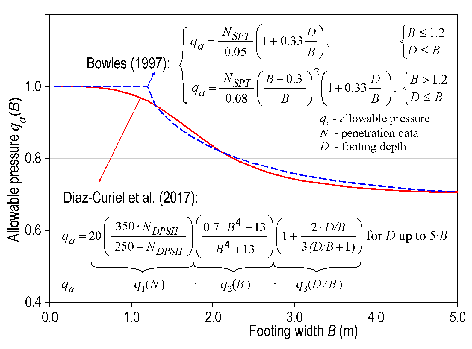
In civil engineering, the resistance of the ground to footing foundations is important for the construction of road structures and buildings. The so-called allowable soil pressure qa is conventionally used to characterise this geomechanical resistance. This parameter provides the pressure which the foundation footings (indeed, the ground) can withstand according to a target structure and without exceeding the subsidence limit determined in the standard formulation (e.g., 25 mm settlement in Part 2 of Eurocode 7 for geotechnical design). This standard also includes the widespread Bowles relation [26], which relates qa with penetrometric data N, footing radio B, and embedment D as the standard equation. However, these standard equations have two flaws. (1) Two different expressions are required depending on the footing dimensions, which involve unnatural discontinuities. (2) These equations are only valid up to a depth that is limited by the footing width. The empirical data from which the conventional relationships are derived show that the ground subsidence gradually changes from a relatively constant behaviour to a critical value from which the ground tends asymptotically to a different constant value. This can lead to the conclusion that the footing is supported on the ground up to a certain size but sinks into the ground beyond that size, resulting in a different response behaviour. From a theoretical point of view, it would, therefore, be possible to search for a function that reflects both behaviours with a corresponding continuous transition between them.
To adequately resolve these issues, Díaz-Curiel et al. [5] modified the standard formula for calculating the allowable pressure value as a function of footing width, among other variables. Figure 3 shows the comparison between the resulting curve from the two existing relationships with discontinuous gradients and the resulting curve from the new single relationship with continuous gradients. This new formulation also makes it possible to establish a single parameter q1(N) that includes a new relationship between NSPT (obtained by the standard penetration test in boreholes) and the more extensively used NDPSH (obtained by the dynamic penetration test). This parameter is independent of footing and reflects the terrain characteristics that affect its allowable pressure. A new relationship q3(D/B) was also developed to evaluate the variation of the allowable pressure for appreciably greater depths than the footing width. Thus, correcting the continuous increasing linear expression (1 + 0.33·D/B) from Terzaghi and Peck [27], established for D < B, on the influence of D/B for allowable pressure values. The three relationships q1(N), q2(B), and q3(D/B) were developed using the y2A(x) function.
3.2. Nuclear Magnetic Resonance Soundings
The application of nuclear magnetic resonance (NMR) is widely accepted in many fields (e.g., medicine), and its application and validity for the characterisation of geological media have increased in recent decades. Apart from the technological advances that have allowed its implementation, NMR values allow estimating some properties of the subsurface, such as porosity and permeability. The most relevant formulation is the one that allows an estimation of medium permeability from the free porosity Ømr obtained using NMR, , where C is an adjustment factor, t1 is the NMR relaxation time, and p is an exponent with two possible values. These two values come from the fact that the relationship knmr(Ø,t1) has two distinct sources: (1) a theoretical–empirical origin [28], which concludes that p = 1; and (2) a purely empirical character [29], which concludes that the best fit is obtained for p ≈ 4. Clearly, the selection of either exponent value radically alters the obtained results; thus, the values of C vary by several orders of magnitude, which greatly reduces the application of the NMR technique for estimating permeability.
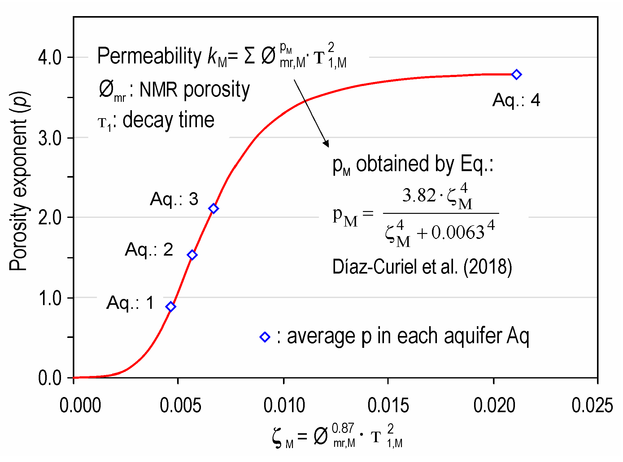
Under the hypothesis that this exponent is a characteristic parameter of each geological medium, Díaz-Curiel et al. [6] resolved this limitation by developing an empirical relationship to obtain this exponent in unconsolidated detrital media. The exponents that yield a minimum deviation with respect to the directly measured hydraulic data were obtained for each aquifer using the empirical data of 23 magnetic resonance soundings measured in four detrital aquifers of four continental basins. Because the p values do not correlate well with any of the parameters provided by the NMR technique, a new variable ζM was defined: , where Ømr,M and t1,M denote the average Ømr and t1 values in each aquifer, respectively, and h is an adjustment coefficient close to 1. ζM provides a high correlation (R2 = 0.95) with the empirical data, and the fitting to a monotonic function reaches a maximum for h = 0.87. The developed function of double asymptote (Figure 4) presents a mean deviation of 1.5%. The function of double asymptote obtained thus provides the expected asymptotic values, which would not have been otherwise obtained using linearisable functions. The determination of h and the coefficients of the developed relationship in other geological media will allow this relationship to be applicable to any porous lithology; thus, it could be considered a general empirical law or its application range is limited to unconsolidated detrital formations.
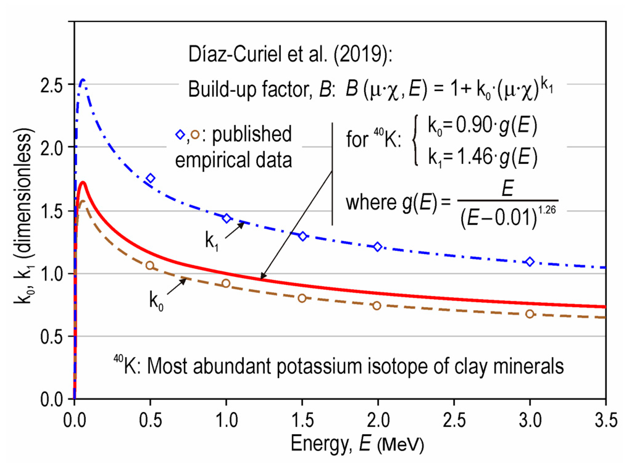
3.3. Correction of Gamma-Ray Well Logs
The knowledge of natural radioactivity is important not only for localising radioactive mineral deposits for nuclear energy use but also for quantifying the percentage of clay contained in many sedimentary formations, which strongly influences the medium permeability. A representative case of subsurface characterisation involves the measurement of gamma radioactivity in boreholes.
Radioactive nuclides undergo a series of collisions with each other and other particles in a medium during their displacement. This produces two different effects: (1) attenuation when the particles are transformed in these collisions and (2) build-up in certain spatial areas owing to the trajectory deviations. The geometry of the source-detector system also affects the measurements, whose correction is conventional in laboratory processes. However, the environmental conditions are highly variable when measuring natural radioactivity in boreholes. Thus, empirical charts were used until 2018 for each set of environmental conditions and probes.
This led to the development of several empirical relationships to quantify the attenuation and accumulation that occurs in cylindrical sources towards their interior (axis). In this case, the empirical relationships developed by Díaz-Curiel et al. [7] not only provided analytical expressions to obtain the clay content but also implemented the accumulation effect, which had not been previously considered. This effect was not addressed in studies that attempted to establish a solution using Monte Carlo modelling, which focused on empirical relationships to obtain the effective distances for application in the radiation attenuation and accumulation equations when propagating through a cylindrical medium from the outside to the inside. That work concluded with formulas fitted to the historically used empirical charts. In addition to the application in wells, the relationships developed for this geometry in their inverse form are of great interest in the study of geological repositories of radioactive waste containers. However, these are admittedly specific applications.
Nevertheless, in the procedure of arriving at these relationships, an empirical relationship must be included to reflect the sharp reduction to zero of the radioactive build-up as a function of energy at very low energies (Figure 5). Although the energy values of radioactive nuclides in nature are considerably higher than 0.1 MeV, without this consideration, the energy dependence would establish that the accumulation of radiation grows asymptotically toward ∞ when approaching very low energies, which has no physical meaning.
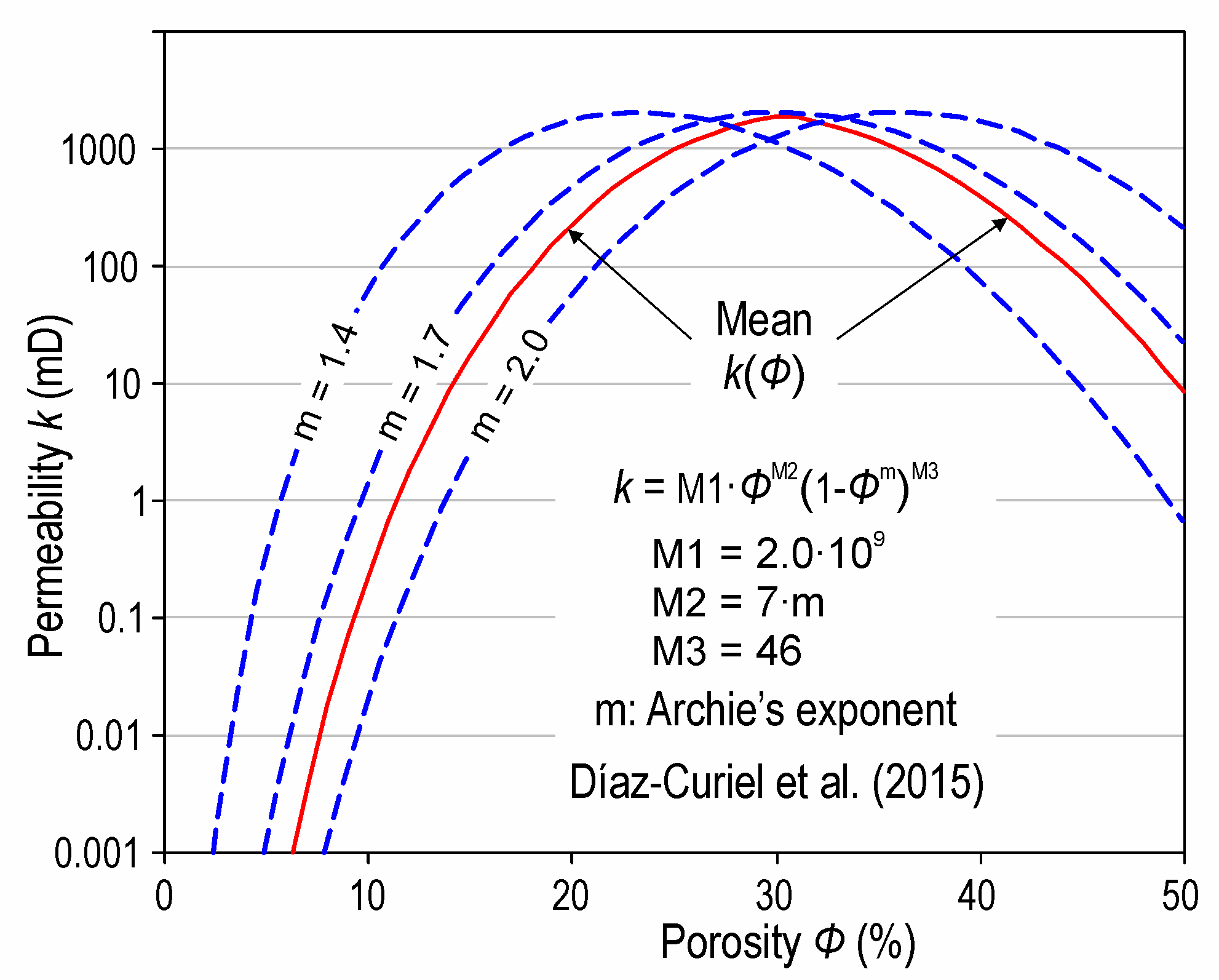
3.4. Porosity/Permeability Relationship in Granular Porous Media
The relationship between permeability (k) and porosity (Ø) in natural porous media is an important foundation in petrophysics. For granular media, in particular, porosity values mostly range between 0% and 50%, with ~25% representing a very significant structural difference between cemented and unconsolidated media. Prior to 2015, there were two ways to understand the k(Ø) relationship. In the petroleum field, the general idea was that porosity and permeability are positively correlated in granular media, which was reflected in a large number of publications on cemented rocks. However, in the field of hydrogeology, it was widely known that the correlation is negative in unconsolidated granular media. This disagreement was not resolved even though one of the most accepted relationships for estimating permeability is the equation of Kozeny [21], according to which the permeability of a medium of smaller grain size (clay–silt) is lower than those in media with larger grain sizes (sand–gravel). It should be noted that both cemented media with low Ø and unconsolidated media with high Ø have smaller grain sizes.
A continuous relationship was presented in Díaz-Curiel et al. [3] that encompasses cemented to unconsolidated formations (Figure 6) and is a function of a well-known parameter in petrophysics: the exponent m of the porosity in Archie’s first law (F = 1/Øm). This exponent is referred to as the cementation coefficient owing to the large number of publications in the petroleum literature, even though it also applies to unconsolidated formations. In this case, the developed fitting function has vertical asymptotes for Ø = 0 and Ø = 1 and is thus a modified y2A(Ø) formula.
This is a good example to understand to what extent an existing expression, a model based on ideal configurations, or laboratory measurements limited to specific lithologies may or may not be useful to cover a geological reality. That would be the case where the variety of behaviours can only be expressed by relationships from a completely empirical point of view. It should be noted that some lithologies have characteristics that strongly differ from those of most granular formations, such as certain volcanic rocks (e.g., pumice) and karst formations (e.g., fractured limestone).
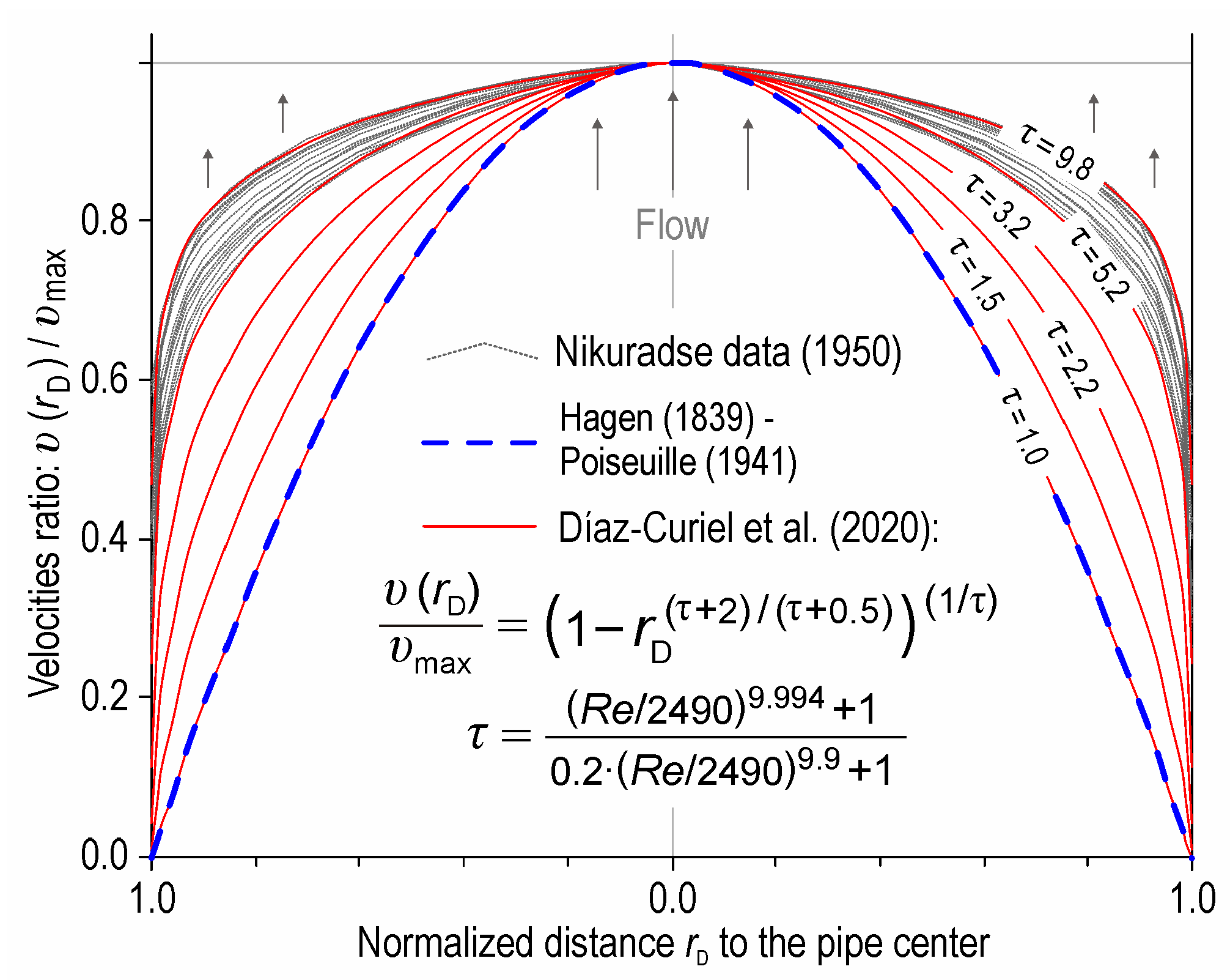
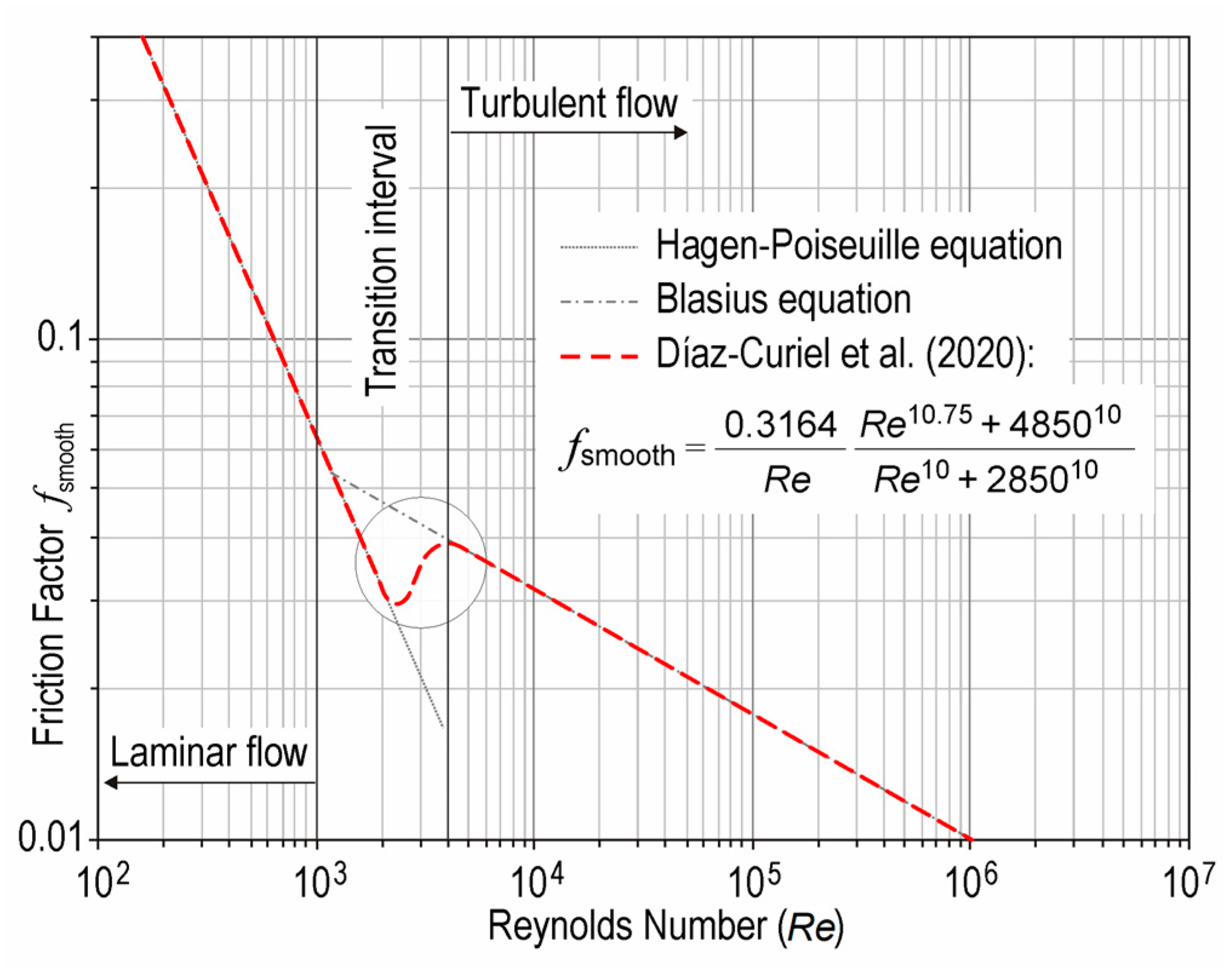
3.5. Continuous Relationship for Laminar Flow to Turbulent in Hydraulics
The importance of the flow characteristics of water and hydrocarbons is recognised for all transport networks through circular conduits (pipes). The capillary model is the most commonly used approach to understand flow behaviour in the geological porous media of the subsoil. Knowledge of the relations governing these flows through circular channels is a crucial aspect that presents a particularly differentiated behaviour between low-velocity (laminar) and high-velocity (turbulent) regimes. The transition interval between these two flow regimes is neither a strictly continuous step nor discontinuous. In laminar flow, the fluid advances homogeneously along the channel length and width; when the flow is completely turbulent, the fluid becomes homogeneously disordered. Spatial and temporal heterogeneities arise within the transition interval, and different results can be obtained from instantaneous images or punctual measurements. The formulation applied until 2020 relatively disregarded the transition interval between these regimes, particularly its effects on two crucial parameters for hydraulic calculations: (1) the ratio of the axial distribution of the flow velocity inside the pipes to velocity in the axis v(rD)/vmax (the velocity law), and (2) the friction factor in smooth pipes fsmooth, for which there were no applicable relationships in the transition interval between the two flows. In Díaz-Curiel et al. [4], relationships for both parameters were presented for the velocity law as a function of the turbulence exponent τ (Figure 7) and for the friction factor as a function of the Reynolds number Re (Figure 8). Thus, the previous transition interval ambiguity of the conventional equations was solved, providing expressions that continuously reflect the fluid flow behaviour for any regime.
The main problem we encountered was that, in general, the characterisation of the transition interval had been underestimated. This contrasts with the fact that the interpolation between laminar and turbulent flow is supported from an experimental point of view in the classical and most recent widespread studies, and its convenience was predicted by well-known authors (referred to in that publication). Although, in this case, the two generated laws show that both phenomena can be represented by a double-asymptote dependence, the one shown by the velocity law is particular because it deals with the radial behaviour of the friction attenuation phenomenon as a function of the distance to the wall.
4. Discussion
Considering that the y2A(x) functions do not consist of functions of multiple non-periodic inflexions but involve two distinct trends along the x-axis, the way used to assume that such a mathematical expression is able to reflect these two trends has been to show a series of examples of which this double behaviour is known in geosciences and in which the fit obtained is sufficiently precise.
Next, some possible concerns about the development of new empirical relationships are discussed. This discussion does not include debates on each of the presented examples, as the differences with existing relationships were added in each of the corresponding publications.
A first possible objection might be that only in a relatively small number of cases the empirical relationship between two or more parameters is purely based on the observation of a statistical correlation. However, the above representative cases of empirical relationships between two quantities have already shown, based on the observation of a statistical correlation and the criteria for its development detailed in Section 2, to improve certain existing relationships, and nowhere in this study is it claimed that this occurs in all cases. In some phenomena that occur in geological environments, the number of variables may be very high. Theoretically, quantifying the effect of each is then very complex, making it necessary first to consider the existence of relationships that comprise the entire set of data (see [3]).
A possible second reproach might be that deviations between empirical data and existing relationships derived from well-known theoretical models are attributable to the lack of knowledge of some involved parameters. However, it would be lax to use this argument to dismiss the new empirical relationships rather than the existing theoretical equations unless it were true that this is the case in the new relationships rather than in the existing ones. By way of example, it might be thought that there is a one-to-one relationship between permeability and porosity in fractured rocks such that the deviations between empirical data and existing relationships would be due to a lack of knowledge of the statistical distribution of fractures and their extent and connectivity. However, it is known that there is no unique dependence between permeability and porosity, so it is that assumption that fails in this case. Conversely, if in the development of a new empirical relationship, the formation factor of a fractured rock is considered to comprise these overlooked variables, this should lead to the acceptance of this new law, even if it is empirical in origin. Indeed, it may be that such dependence has not been analysed to date for fractured rocks, as is the case of the porosity/permeability relationship in granular porous media shown in this study.
The third possible disapproval might be that empirical laws allow comparing substantially different phenomena from a physical point of view, such as the correlation between strength features and stress–strain behaviour. In the case of the relationship between strength and Young’s modulus in soils, these may appear to be two substantially different phenomena to those that do not consider the degradation of this characteristic with respect to the load to which a soil is subjected. The same may be said for the relationship between NSPT (dynamic penetration data) and seismic wave velocities (vS and vP) in soils, which are different phenomena, as they consider very different degrees of deformation. However, if it is considered that the deformation of the modulus with load in granular soils follows an evolution closely related to the granulometric grading coefficient, a correlation relationship can be found between NSPT and vs. and vP that involves these two degrees of deformation (see [5]). In other words, the new empirical law would establish that in soils, degradation of static moduli with strength remains statistically correlated with the granulometric grading coefficient.
In the case of existing empirical relationships, even those based on partial theoretical knowledge of a studied phenomenon, an anticipated discrepancy might be the argument that their replacement with new relationships that have no theoretical basis might not be appropriate, even when the latter provides a better data fit. In this regard, it should be noted that the aim of this study is not to criticise theoretical laws but to point out the possibilities of empirical laws in some cases. In fact, partial knowledge of a given phenomenon may have caused some theoretical laws to diverge from the empirical data. One such case, even including the development of a theorem [33], would be not considering the accumulation in the dispersion of gamma radiation inside the wells, producing results far from the empirical values for large well diameters (see [7]). Another case would be the misconception produced in the conventional expression of the formation factor F* for clay-containing media. Waxman and Smits [34], starting from σ0 = kx·σc + ky·σw, where σ0, σc, and σw are the conductivities of a sample, clay exchange cations, and salt solution in equilibrium, respectively, and kx and ky are the appropriate geometric factors. Then, they assumed that the geometric factor is the inverse of the formation factor (according to their equation, kx = ky = 1/F*). This is not appropriate, as the formation factor would vary with, for example, the length of the sample (see [3]).
Finally, a possible objection might be that the function of double asymptote y2A(x) is independent of the mechanics of the underlying phenomenon and does not provide any information in this regard. First, this objection would rule out the interest for calculations in industrial applications of having a suitable relationship that allows a much more precise calculation of the parameter value under analysis, as in the case of the admissible pressure in buildings or the determination of the flow velocity that minimises the transport cost in macro-installations such as refineries. Secondly, it has already been stated in this study that obtaining a well-adjusted empirical formula allows, by itself, the search for and development of appropriate theoretical formulas. That is, starting from a function of double asymptote y2A(x), algebraic operations can be performed that transform this function into the product or sum of two different functions that reflect the two behaviours established in the developed y2A(x) function. This is especially valid if the ranges of the domain under consideration are representative of the whole phenomenon and if the asymptotic trends are the expected ones, as in the examples shown in this study. It should be borne in mind that many of the theoretical-empirical relationships are based on an improperly applied theoretical analogue, and it is precisely the fact of developing an analytical relationship of empirical origin that makes it possible to think that the model is incorrect. This occurs, for example, in the case of tortuosity, both for having conventionally used a relationship that has nothing to do with the real tortuosity of the flow and for having used the straight capillary model, which is not applicable in isotropic granular media (see [13]). Thus, the existing equations for granular media derived from the Poiseuille equation [10] should not be considered an adequate theoretical development, and nor should Maxwell’s model for mixtures of suspended particles have been applied to solid media (see [13]). For all these, it is precisely the fact of developing an analytical relation of empirical origin that makes it possible to think that the existing model is incorrect. It is finally interesting to note that there are other functions of double asymptote that have already been accepted by the fact that they have already been applied, such as, for example, the functions derived from the logistic law [35].
5. Conclusions
The presented examples affirm that it is still necessary to investigate certain phenomena in geosciences to obtain new empirical laws that synthesise their dependencies and behaviour. The main differences in the presented formulas compared with the results of previous research in the literature are included in the background and discussion sections of the related papers. In some of the presented examples, the previous equations are quite a few years old, which shows that there may be certain reservations about entering into scientific debates in these types of cases, which is a contradiction, given that science advances precisely by questioning our knowledge.
The empirical laws presented in this paper demonstrate that the y2A(x) functions faithfully reflect the behaviour of certain geoscience phenomena, accurately fitting with the empirical data. The applied character of the presented examples supports the validity of the empirical laws. When such laws are well established, they can be used to minimise the influence of measurement errors, more realistically reflect the main characteristics of analysed phenomena, and ultimately determine possible theoretical laws.
The remaining question would be to find a theoretical explanation that justifies that this function comes from considering a double behaviour as the value of the analysed parameter increases, regardless of whether arguments are presented on the physics of these differentiated trends.
Author Contributions
Conceptualization, J.D.-C.; methodology, J.D.-C.; validation, J.D.-C. and L.A.-L.; formal analysis, J.D.-C. and B.B.; resources, L.A.-L., D.P.-P. and M.J.M.; writing—original draft preparation, J.D.-C., B.B. and L.A.-L.; writing—review and editing, D.P.-P. and M.J.M.; visualization, J.D.-C. and D.P.-P.; supervision, J.D.-C.; funding acquisition, J.D.-C. and B.B. All authors have read and agreed to the published version of the manuscript.
Funding
Part of this study was supported by the “Comunidad de Madrid” Regional Government of Madrid, Spain, grant number CARESOIL-CM P2018/EMT-4317.
Institutional Review Board Statement
Not applicable.
Informed Consent Statement
Not applicable.
Data Availability Statement
Not applicable.
Conflicts of Interest
The authors declare no conflict of interest.
References
- Godoy, V.A.; Napa-García, G.F.; Gómez-Hernández, J.J. Ensemble smoother with multiple data assimilation as a tool for curve fitting and parameter uncertainty characterization: Example applications to fit nonlinear sorption isotherms. Math. Geosci. 2022, 54, 807–825. [Google Scholar] [CrossRef]
- Nigmatullin, R.; Dorokhin, S.; Ivchenko, A. Generalized Hurst Hypothesis: Description of Time-Series in Communication Systems. Math 2021, 9, 381. [Google Scholar] [CrossRef]
- Díaz-Curiel, J.; Biosca, B.; Miguel, M.J. Geophysical Estimation of Permeability in Sedimentary Media with Porosities from 0 to 50%. OGST—Rev. D’ifp Energ. Nouv. 2015, 71, 18. [Google Scholar] [CrossRef]
- Díaz-Curiel, J.; Miguel, M.J.; Caparrini, N.; Biosca, B.; Arévalo-Lomas, L. Improving some Basic Relationships of Pipe Hydraulics. Application for Processing Flowmeter Logs in Water Wells. Flow Meas. Instrum. 2020, 72, 101698. [Google Scholar] [CrossRef]
- Díaz-Curiel, J.; Rueda-Quintero, S.; Biosca, B.; Doñate-Matilla, G. Advance in the penetrometer test formulation to estimate allowable pressure in granular soils. Acta Geotech. 2017, 12, 1119–1127. [Google Scholar] [CrossRef]
- Díaz-Curiel, J.; Biosca, B.; Doñate-Matilla, G.; Rueda-Quintero, S. Estimation of hydraulic transmissivity from MRS by varying the porosity exponent, in detrital aquifers of the Iberian Peninsula. Near Surf. Geophys. 2018, 16, 401–410. [Google Scholar] [CrossRef]
- Díaz-Curiel, J.; Miguel, M.J.; Biosca, B.; Medina, R. Environmental correction of gamma ray logs by geometrical/empirical factors. J. Pet. Eng. 2019, 173, 462–468. [Google Scholar] [CrossRef]
- Darcy, H. Détermination des Lois D’écoulement de l’eau a Travers le Sable. Les Fontaines Publiques de la Ville de Dijon, Appendis, Note D; Dalmont, V., Ed.; Paris, France, 1856; pp. 590–594. [Google Scholar]
- Archie, G.E. Introduction to petrophysics of reservoir rocks. AAPG Bull. 1950, 34, 943–961. [Google Scholar]
- Poiseuille, J.L. Recherches Expérimentales sur le Mouvement des Liquides dans les Tubes de Très-Petits Diamètres; Imprimerie Royale: Tournai, Belgium, 1844. [Google Scholar]
- Sundberg, K. Effect of impregnating waters on electrical conductivity of soils and rocks. Trans. Am. Inst. Min. Met. Eng. 1932, 97, 367–391. [Google Scholar]
- Díaz-Curiel, J. Theory and Practice of Geophysical Prospecting; 2000; ISBN 978-84-692-7448-4. [Google Scholar]
- Díaz-Curiel, J.; Biosca, B.; Arévalo-Lomas, L.; Miguel, M.J. Failure of the Conventional Expression of Tortuosity in Granular Porous Solids. Surv. Geophys. 2021, 42, 943–960. [Google Scholar] [CrossRef]
- Colebrook, C.F. Turbulent flow in pipes with particular reference to the transition region between the smooth and rough pipe laws. J. Inst. Civil Eng. 1939, 11, 133–156. [Google Scholar] [CrossRef]
- Di Maio, R.; Piegari, E. Water storage mapping of pyroclastic covers through electrical resistivity measurements. J. Appl. Geophy. 2011, 75, 196–202. [Google Scholar] [CrossRef]
- Di Maio, R.; Piegari, E.; Todero, G.; Fabbrocino, S. A combined use of Archie and van Genuchten models for predicting hydraulic conductivity of unsaturated pyroclastic soils. J. Appl. Geophy. 2015, 112, 249–255. [Google Scholar] [CrossRef]
- He, M.M.; Pang, F.; Wang, H.T.; Zhu, J.W.; Chen, Y.S. Energy dissipation-based method for strength determination of rock under uniaxial compression. Shock Vib. 2020, 2020, 8865958. [Google Scholar] [CrossRef]
- Tisato, N.; Madonna, C.; Saenger, E.H. Attenuation of seismic waves in partially saturated Berea sandstone as a function of frequency and confining pressure. Front. Earth Sci. 2021, 9, 641177. [Google Scholar] [CrossRef]
- Nigmatullin, R.R.; Bataleva, E.A.; Nepeina, K.S.; Matiukov, V.E. Quality control of the initial magnetotelluric data: Analysis of calibration curves using a fitting function represented by the ratio of 4th-order polynomials. Measurement 2023, 216, 112914. [Google Scholar] [CrossRef]
- Yu, Y.; Loskot, P. Polynomial Distributions and Transformations. Measurement 2023, 11, 985. [Google Scholar] [CrossRef]
- Kozeny, J. Uber die kapillare leitung des wassers im boden-aufstieg versickerung und anwendung auf die bewässerung, Sitzungsberichte der Wiener Akademie der Wissenschaften. Math. Naturwiss (Abt. IIa) 1927, 136, 271–306. [Google Scholar]
- Díaz-Curiel, J.; Miguel, M.J.; Biosca, B.; Arévalo-Lomas, L. New granulometric expressions for estimating permeability of granular drainages. Bull. Eng. Geol. Environ. 2022, 81, 397. [Google Scholar] [CrossRef]
- Kleinberg, R.L.; Horsfield, M.A. Transverse relaxation processes in porous sedimentary rock. J. Magn. Reson. (1969) 1990, 88, 9–19. [Google Scholar] [CrossRef]
- Díaz-Curiel, J.; Biosca, B.; Arévalo-Lomas, L.; Miguel, M.J.; Loayza-Muro, R. On the Validity of the Relationship 1/T= 1/TB+ 1/TS+ 1/TD in NMR Techniques with Regards to Permeability Estimation of Natural Porous Media. Front. Earth Sci. 2021, 9, 688686. [Google Scholar] [CrossRef]
- Díaz-Curiel, J. Interpretación y correlación automáticas de diagrafías geofísicas. Aplicación a la hidrogeología en el sur de la Cuenca del Duero. Ph.D. Thesis, Universidad Politécnica de Madrid, Madrid, Spain, 1995. [Google Scholar] [CrossRef]
- Bowles, J.E. Foundation Analysis and Design, 5th ed.; McGraw-Hill: Singapore, 1997. [Google Scholar]
- Terzaghi, K.; Peck, R.B. Soil Mechanics in Engineering Practice, 2nd ed.; Wiley: New York, NY, USA, 1967. [Google Scholar]
- Seevers, D.O. A nuclear magnetic method for determining the permeability of sandstones. In Proceedings of the Transactions on SPWLA 7th Annual Logging Symposium, Houston, TX, USA, 9–13 June 1966. [Google Scholar]
- Kenyon, W.E.; Day, P.I.; Straley, C.; Willemsen, J.F. A three-part study of NMR longitudinal relaxation properties of water-saturated sandstones. SPE Form. Eval. 1988, 3, 622–636. [Google Scholar] [CrossRef]
- Nikuradse, J. Gesetzmässigkeiten der Turbulenten Strömung in Glatten Rohren. In Forschung auf dem Gebiete des Ingenieurwesens, No. 356; Laws of Turbulent Flow in Smooth Pipes; VDI: Berlin, Germany, 1932; Volume 3, pp. 1–76. [Google Scholar]
- Hagen, G. Über Die Bewegung des Wassers in engen zylindrischen Röhren [About the Movement of Water in Narrow Cylindrical Pipes]. Poggendorfs Ann. Phys. Und Chem. 1839, 16, 423–442. [Google Scholar] [CrossRef]
- Blasius, H. Das Ähnlichkeitsgesetz bei Reibungsvorgängen in Flüssigkeiten [The law of similarity in friction processes in fluids]. Forschungs-Arbeit des Ingenieur-Wesens. In Mitteilungen über Forschungsarbeiten auf dem Gebiete des Ingenieurwesens: Insbesondere aus den Laboratorien der Technischen Hochschulen; Springer: Berlin/Heidelberg, Germany, 1913; p. 131. [Google Scholar] [CrossRef]
- Wahl, J.S. Gamma Ray Logging. Geophysics 1983, 48, 1536–1550. [Google Scholar] [CrossRef]
- Waxman, M.H.; Smits, L.J.M. Electrical conductivities in oil bearing shaly sands. Soc. Pet. Eng. J. 1968, 243, 107–122. [Google Scholar] [CrossRef]
- Derron, M.H.; Jaboyedoff, M. Preface LIDAR and DEM techniques for landslides monitoring and characterization. Nat. Hazards Earth Syst. Sci. 2010, 10, 1877–1879. [Google Scholar] [CrossRef]
Figure 1.
Limitation of fitting functions using least squares: (○) 23 data points obtained from the exponential function y = 10·e−0.2x, (×) the same data series except for a very outlier y at the lowest x, and (−·−·−) fitting function to the (×) series; (◊) 23 data points obtained from the power function y = 0.1·x2, (+) the same data series except for a very outlier y at the lowest x, and (- - -) fitting function obtained by least squares to (+) series.

Figure 2.
Examples of functions y2A(x): (a) Cases with one principal curvature (concave or convex). (b) Cases with two or more curvatures. (c) Plot of data series from which the functions f01, f03, y f05 in (a) are obtained in addition to the exponential or potential best fit to root mean square (RMS) curves. (d) Cases with equal exponents equal and c2 = c3.

Figure 3.
Allowable pressure qa of soils according to Bowles [26] (dashed line) and according to Díaz-Curiel et al. [5] (solid line).

Figure 4.
Porosity exponent to estimate permeability using the NMR technique [6].
Figure 4.
Porosity exponent to estimate permeability using the NMR technique [6].

Figure 5.
Radioactivity build-up factor for a mass attenuation coefficient μ and effective distance χ [7].
Figure 5.
Radioactivity build-up factor for a mass attenuation coefficient μ and effective distance χ [7].

Figure 6.
Porosity/permeability relationship in granular porous media for Ø = 0–50% [3].
Figure 6.
Porosity/permeability relationship in granular porous media for Ø = 0–50% [3].

Figure 7.
Velocity profile of fluid flow in capillaries for different turbulence exponents τ according to Díaz-Curiel et al. [4] (red lines), Nikuradse [30] data (grey lines), and velocity profile for laminar flow since the Hagen–Poiseuille [10,31] equation (blue dashed line).

Figure 8.
Friction factor of fluid flow in smooth-walled capillaries since Díaz-Curiel et al. [4] (red line), according to the Hagen–Poiseuille [10,31] equation for laminar flow (dashed grey line), and according to Blasius [32] for turbulent flow (dotted grey line).


| f01 | f02 | f03 | f04 | f05 | f06 | f07 | f08 | f09 | f10 | f11 | f12 | f13 | f14 | |
|---|---|---|---|---|---|---|---|---|---|---|---|---|---|---|
| c1 | 0.1 | 0.04 | 1.0 | 1.0 | - | 2.5 | 2.0 | 1.5 | −8.0 | −1.5 | 1.6 | 5.4 | −1.0 | −2.7 |
| z1 | 2.0 | 2.5 | 1.0 | 1.0 | - | 0.3 | 4.0 | 4.0 | 4.0 | 4.0 | 4.0 | 4.0 | 4.0 | 4.0 |
| c2 | - | 1.0 | - | 0.5 | 1.0 | - | −7.0 | −2.0 | - | - | - | - | 1.0 | 10.5 |
| z3 | 1.0 | 1.0 | 1.0 | 1.0 | 1.0 | 1.0 | 4.0 | 3.6 | 6.0 | 4.0 | 4.0 | 5.0 | 3.5 | 4.0 |
| c3 | 4.0 | 15.6 | 3.0 | 2.0 | 1.0 | 2.0 | 3.5 | 2.0 | 5.1 | 1.0 | 5.1 | 6.6 | 1.0 | 5.1 |
Disclaimer/Publisher’s Note: The statements, opinions and data contained in all publications are solely those of the individual author(s) and contributor(s) and not of MDPI and/or the editor(s). MDPI and/or the editor(s) disclaim responsibility for any injury to people or property resulting from any ideas, methods, instructions or products referred to in the content. |
© 2023 by the authors. Licensee MDPI, Basel, Switzerland. This article is an open access article distributed under the terms and conditions of the Creative Commons Attribution (CC BY) license (https://creativecommons.org/licenses/by/4.0/).
Share and Cite
MDPI and ACS Style
Díaz-Curiel, J.; Biosca, B.; Arévalo-Lomas, L.; Paredes-Palacios, D.; Miguel, M.J. New Empirical Laws in Geosciences: A Successful Proposal. Appl. Sci. 2023, 13, 10321. https://doi.org/10.3390/app131810321
AMA Style
Díaz-Curiel J, Biosca B, Arévalo-Lomas L, Paredes-Palacios D, Miguel MJ. New Empirical Laws in Geosciences: A Successful Proposal. Applied Sciences. 2023; 13(18):10321. https://doi.org/10.3390/app131810321
Chicago/Turabian StyleDíaz-Curiel, Jesús, Bárbara Biosca, Lucía Arévalo-Lomas, David Paredes-Palacios, and María Jesús Miguel. 2023. "New Empirical Laws in Geosciences: A Successful Proposal" Applied Sciences 13, no. 18: 10321. https://doi.org/10.3390/app131810321
Note that from the first issue of 2016, this journal uses article numbers instead of page numbers. See further details here.