
Validation of a Qualification Procedure Applied to the Verification of Partial Discharge Analysers Used for HVDC or HVAC Networks


 , , , , , , ,
Abstract
:1. Introduction
2. Description of the Qualification Procedure of PD Analysers Diagnostic Tools Used for the Insulation Condition of HVDC and HVAC Grids
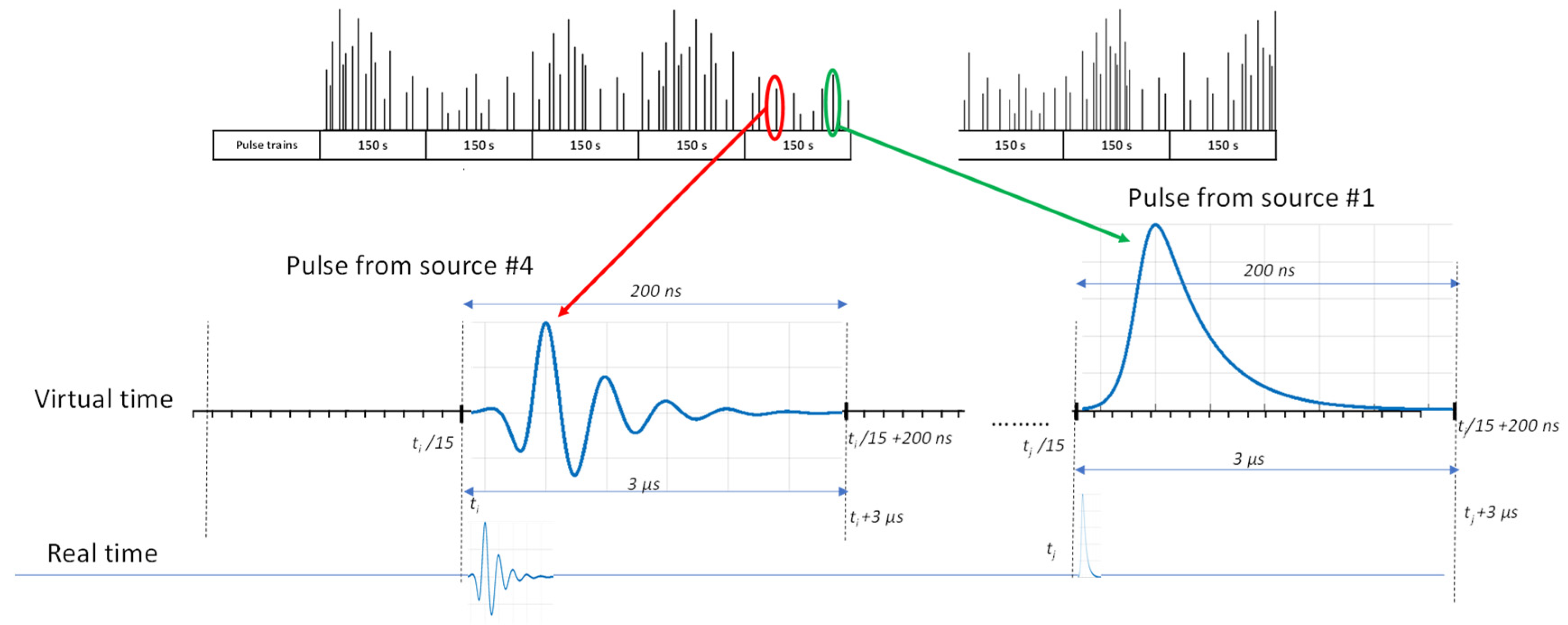
2.1. Reference PD Pulses and Pulsating Noise Trains
2.1.1. PD Pulse Trains in GIS, Cable Systems, and AIS under HVAC Stress
2.1.2. PD Pulse Trains in GIS, Cable Systems, and AIS under HVDC Stress
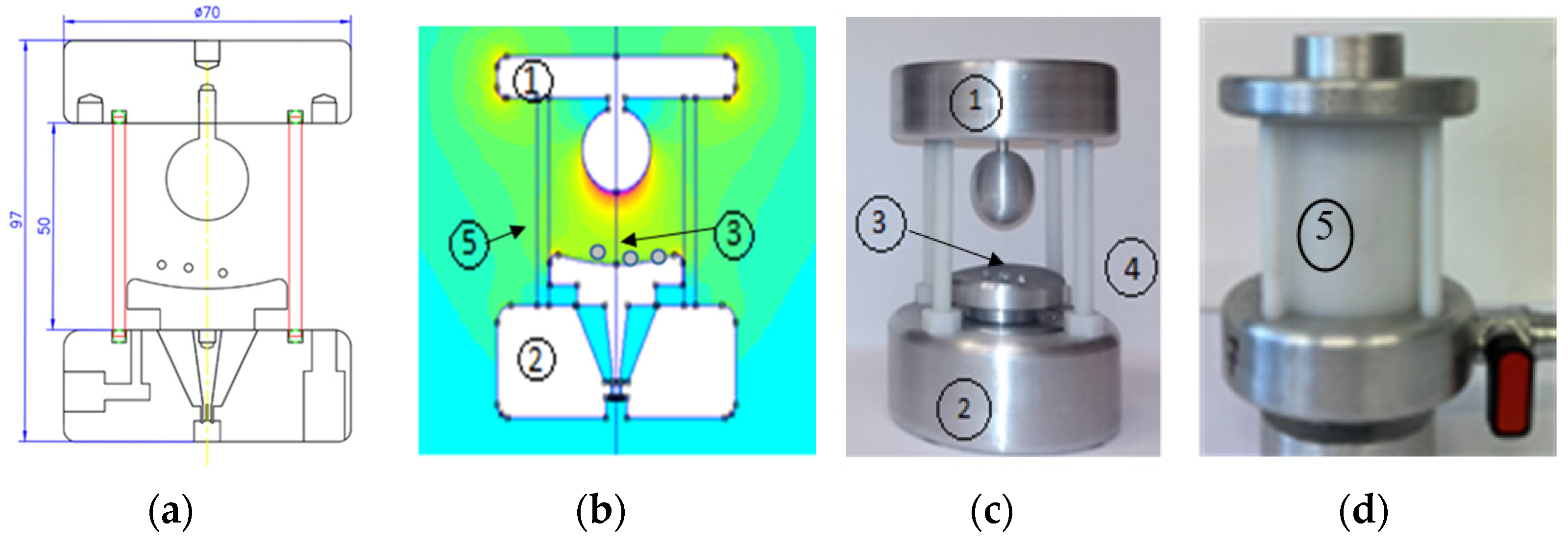
2.1.3. PD Pulse Trains in a Semiconductor Junction Representative of Converters
2.1.4. Noise Pulsating Signals
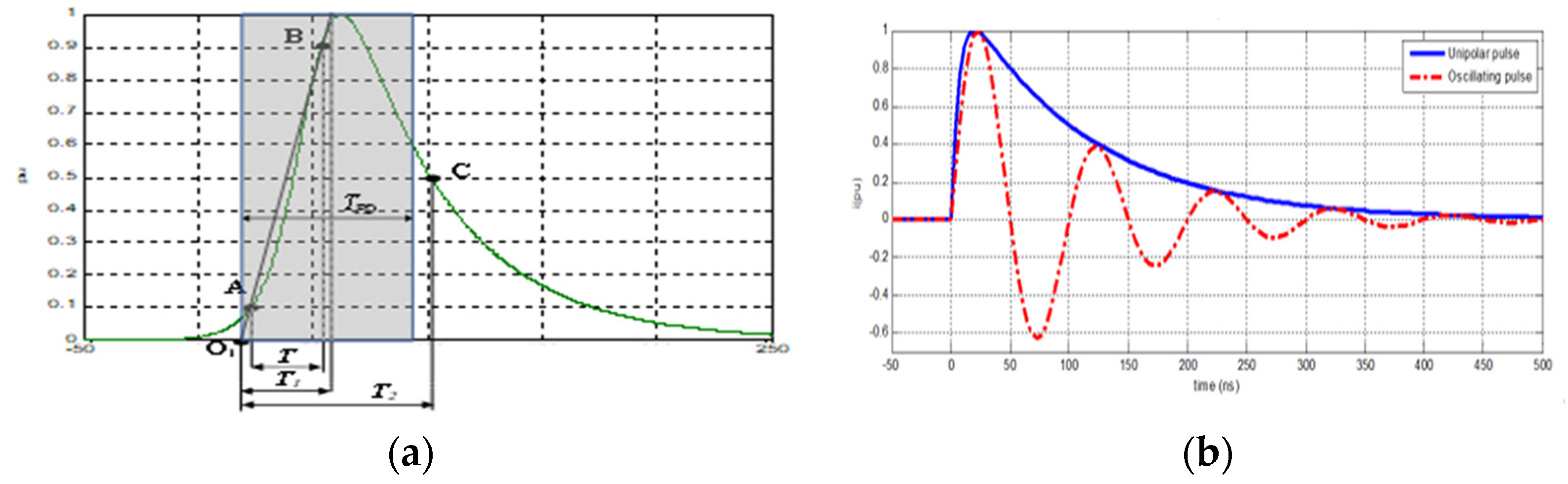
2.1.5. PD Pulse Waveforms
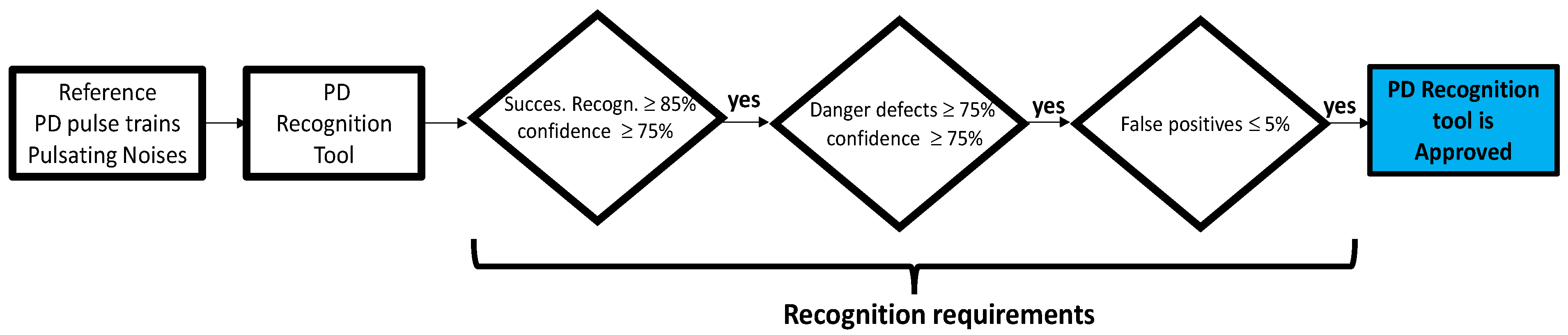
2.2. PD Recognition Test
Requirements to Approve an AI Recognition Tool
2.3. PD Clustering Test
2.3.1. AC Clustering Test
2.3.2. DC Clustering Test
2.3.3. Requirements to Approve an AI Clustering Tool
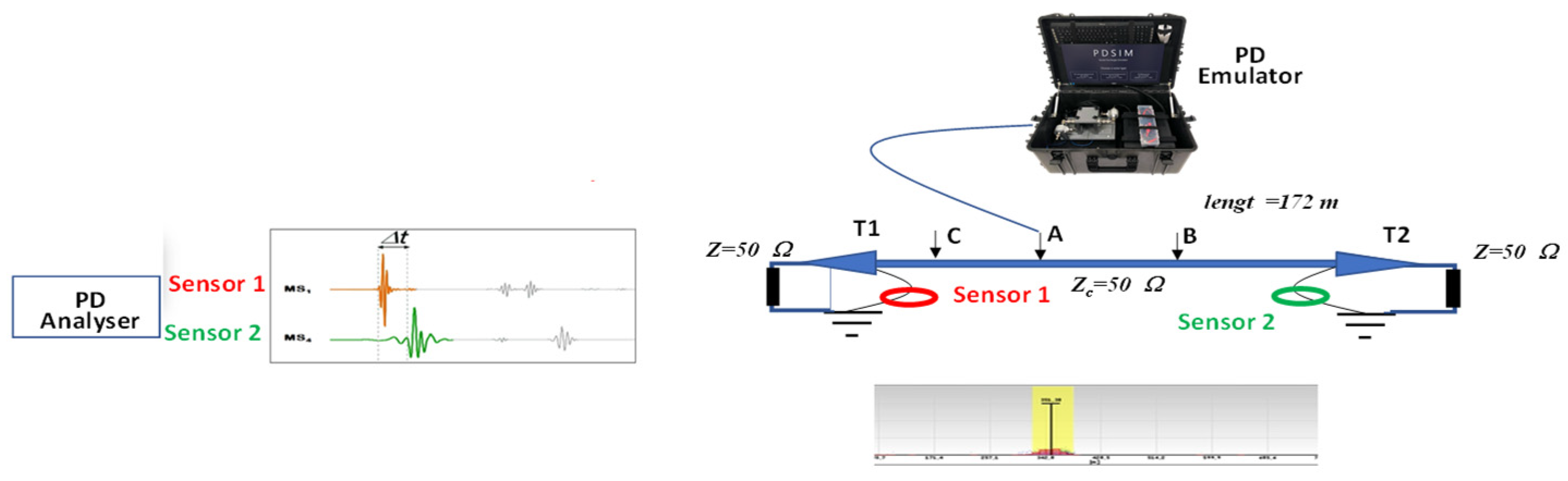
2.4. PD Location Tests for HV Cable Systems
3. PD Recognition Tools for HVAC Insulation Defects Used for a Round Robin Test
3.1. ACR1 Recognition Tool
3.2. ACR2 Recognition Tool
4. PD recognition Tools for HVDC Insulation Defects Used
4.1. DCR1 Recognition Tool
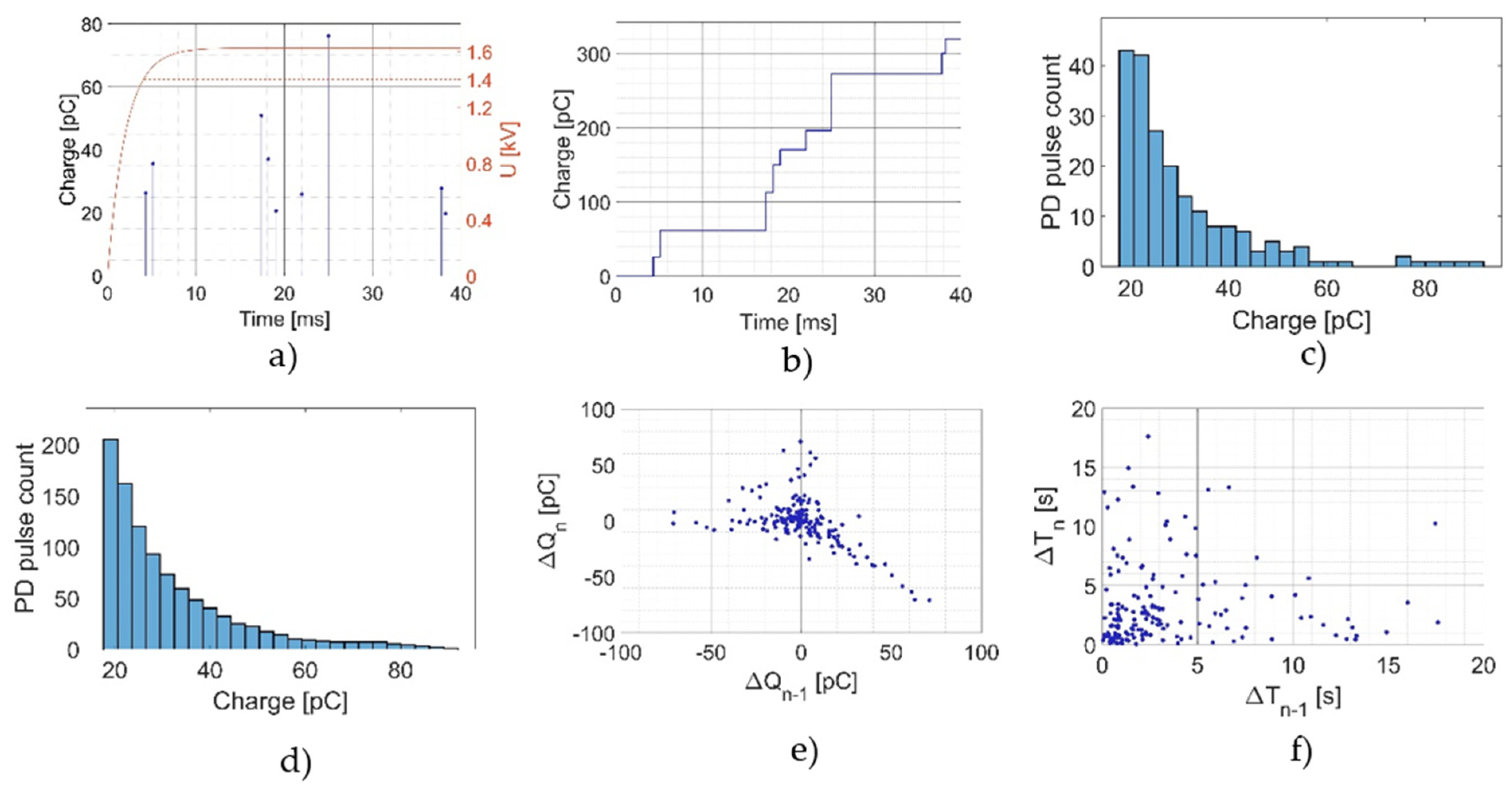
- Δtn−1 vs. Δtn;
- Δqn−1 vs. Δqn;
- PD histogram of charge intervals;
- Amplitude vs. time (PD event train);
- A number of derived quantities were obtained for each test cell, including;
- Maximum, mean, minimum, and standard deviation of amplitude, Δtn, Δqn;
- Kurtosis and skewness.
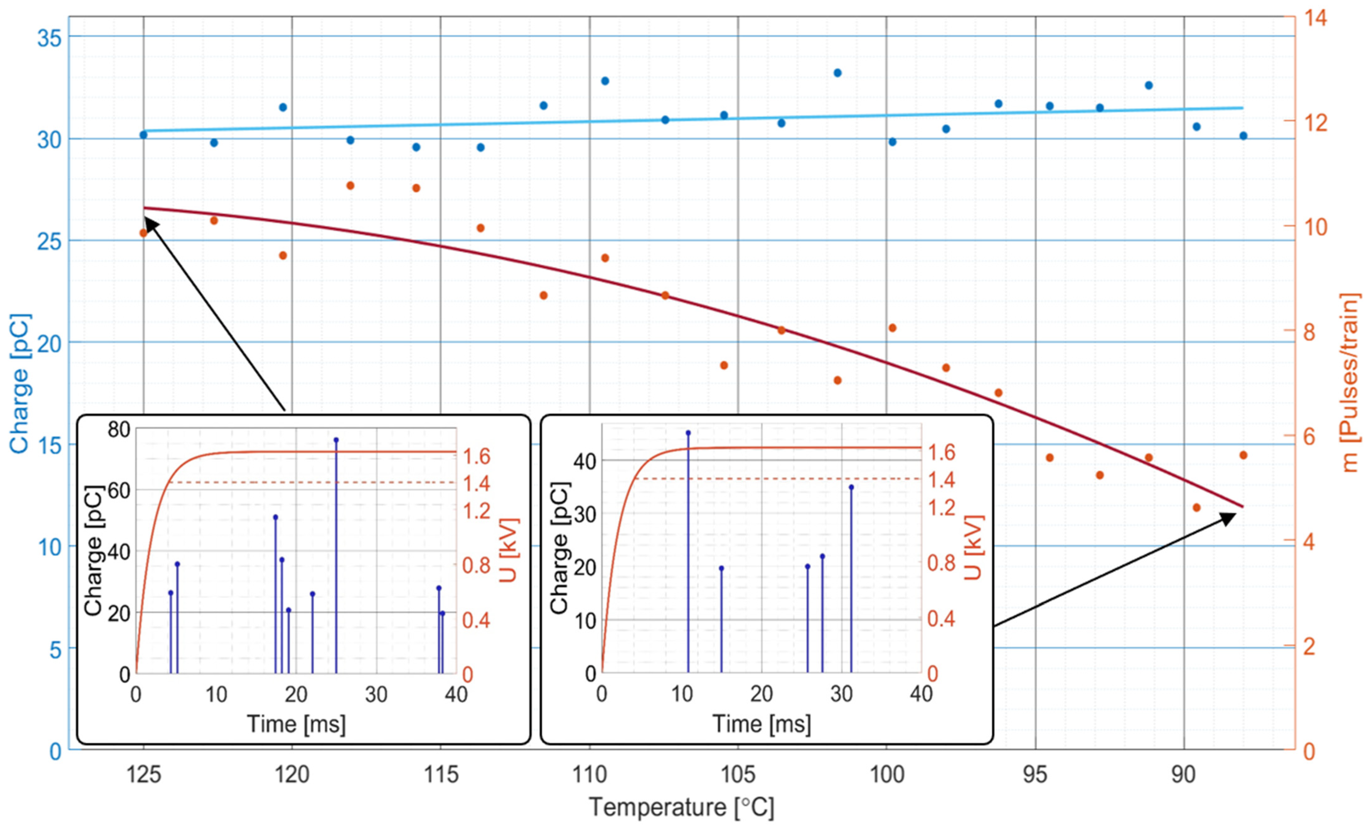
- Number of pulses (high/low),
- Applied voltage,
- Histogram shape (visual interpretation of kurtosis and skewness),
- Visual interpretation of cluster shapes (∆qn−∆qn−1 and ∆tn−∆tn−1),
- Repetitiveness of data (systematic noise).
4.2. DCR2 Recognition Tool
5. Clustering Tools
5.1. C1 Clustering Tool
5.2. C2 Clustering Tool
5.3. Technical Description of a Clustering Tool to Be Applied in the DC Clustering Test
6. Description of the Round Robin Results
6.1. PD Recognition Test Used in the Round Robin Test
6.2. PD Clustering Test
6.3. Results of PD Location Tests
7. Conclusions
Author Contributions
Funding
Institutional Review Board Statement
Informed Consent Statement
Data Availability Statement
Conflicts of Interest
References
- Sahoo, R.; Karmakar, S. Investigation of electrical tree growth characteristics and partial discharge pattern analysis using deep neural network. Electr. Power Syst. Res. 2023, 220, 109287. [Google Scholar] [CrossRef]
- Garnacho, F.; Khamlichi, A.; Álvarez, F.; Ramírez, A.; Vera, C.; Rovira, J.; Simón, P.; Camuñas, A.; Arcones, E.; Ortego, J. Best practices for Partial Discharge Monitoring of HVDC Cable Systems and Qualification Tests. CIGRE Sci. Eng. A Scopus Regist. Mag. (CSE) 2023, 27, 1335–2426. [Google Scholar]
- Álvarez, F.; Garnacho, F.; Ortego, J.; Sánchez-Urán, M.A. Application of HFCT and UHF sensors in on-line partial discharge measurements for insulation diagnosis of high voltage equipment. Sensors 2015, 15, 7360–7387. [Google Scholar] [CrossRef] [PubMed] [Green Version]
- IEC TS 62478:2016; High Voltage Test Techniques—Measurement of Partial Discharges by Electromagnetic and Acoustic Methods. TC 42 High-Voltage and high-Current Test Techniques. International Electrotechnical Commission (IEC) Standards: Geneva, Switzerland, 2016.
- Mashikian, M.S.; Bansal, R.; Northrop, R.B. Location and characterization of partial discharge sites in shielded power cables. IEEE Trans. Power Deliv. 1990, 5, 833–839. [Google Scholar] [CrossRef]
- Steennis, F.; Wagenaars, P.; van der Wielen, P.; Wouters, P.; Li, Y.; Broersma, T.; Harmsen, D.; Bleeker, P. Guarding MV cables on-line: With travelling wave based temperature monitoring, fault location, PD location and PD related remaining life aspects. IEEE Trans. Dielectr. Electr. Insul. 2016, 23, 1562–1569. [Google Scholar] [CrossRef]
- Alvarez, F.; Ortego, J.; Garnacho, F.; Sanchez-Uran, M.A. A clustering technique for partial discharge and noise sources identification in power cables by means of waveform parameters. IEEE Trans. Dielectr. Electr. Insul. 2016, 23, 469–481. [Google Scholar] [CrossRef] [Green Version]
- Perpiñán, O.; Sánchez-Urán, M.A.; Álvarez, F.; Ortego, J.; Garnacho, F. Signal analysis and feature generation for pattern identification of partial discharges in high-voltage equipment. Electr. Power Syst. Res. 2013, 95, 56–65. [Google Scholar] [CrossRef] [Green Version]
- 19ENG02 FutureEnergy “Metrology for future energy transmission” EURAMET H2020 Project, EMPIR Program, 2020-2023.
- Zhang, B.; Ghassemi, M.; Zhang, Y. Insulation Materials and Systems for Power Electronics Modules: A Review Identifying Challenges and Future Research Needs. IEEE Trans. Dielectr. Electr. Insul. 2021, 28, 290–302. [Google Scholar] [CrossRef]
- Mitic, G.; Lefranc, G. Localization of Electrical-Insulation and Partial-Discharge Failures of IGB Modules. IEEE Trans. Ind. Appl. 2002, 38, 175–180. [Google Scholar] [CrossRef]
- Ghassemi, M. PD measurements, failure analysis, and control in high-power IGBT modules. High Voltage 2018, 3, 170–178. [Google Scholar] [CrossRef]
- IEC 61287-1:2014; Power converters installed on board rolling stock—Part 1: Characteristics and test methods.
- Koltunowicz, W.; Plath, R. Synchronous multi-channel PD measurements. IEEE Trans. Dielectr. Electr. Insul. 2008, 15, 1715–1723. [Google Scholar] [CrossRef]
- Wang, Y.; Chen, P.; Zhao, Y.; Sun, Y. A Denoising Method for Mining Cable PD Signal Based on Genetic Algorithm Optimization of VMD and Wavelet Threshold. Sensors 2022, 22, 9386. [Google Scholar] [CrossRef] [PubMed]
- Ma, X.; Zhou, C.; Kemp, I.J. Automated wavelet selection and thresholding for PD detection. IEEE Electr. Insul. Mag. 2002, 18, 37–45. [Google Scholar] [CrossRef]
- De Oliveira, H.; Chaves, L.; Cunhas, T.; Vasconcelos, F.H. Partial discharge signal denoising with spatially adaptive wavelet thresholding and support vector machines. Electr. Power Syst. Res. 2011, 81, 644–659. [Google Scholar]
- Kyprianou, A.; Lewin, P.L.; Efthimiou, V.; Stavrou, A.; Georghiou, G.E. Wavelet packet denoising for online partial discharge detection in cables and its application to experimental field results. Meas. Sci. Technol. 2006, 17, 2367–2379. [Google Scholar] [CrossRef] [Green Version]
- Cavallini, A.; Montanari, G.C.; Puletti, F.; Contin, A. A new methodology for the identification of PD in electrical apparatus: Properties and applications. IEEE Trans. Dielectr. Electr. Insul. 2005, 12, 203–215. [Google Scholar] [CrossRef]
- Ardila-Rey, J.A.; Martínez-Tarifa, J.M.; Robles, G.; Rojas-Moreno, M.V. Partial discharge and noise separation by means of spectral-power clustering techniques. IEEE Trans. Dielectr. Electr. Insul. 2013, 20, 1436–1443. [Google Scholar] [CrossRef]
- Sánchez, A.; Garnacho, F. Requirements of Artificial Intelligence Platform addressed to Automatic Assessment of Insulation Condition of Indoor and Outdoor Installations through Partial Discharge Monitoring. CIGRE Sci. Eng. A Scopus Regist. Mag. (CSE) 2023, 27, 1–14. [Google Scholar]
- Delft University of Technology, PDFlex. 2023. Available online: http://pdflex.ewi.tudelft.nl/ (accessed on 20 November 2022).
- Rodrigo Mor, A.; Castro Heredia, L.C.; Muñoz, F. New clustering techniques based on current peak value, charge and energy calculations for separation of partial discharge sources. IEEE Trans. Dielectr. Electr. Insul. 2017, 24, 340–348. [Google Scholar]
- Álvarez, F.; Ortego, J.; Garnacho, F.; Sánchez-Urán, M.A. Advanced techniques for on-line PD measurements in high voltage systems. In Proceedings of the 2014 ICHVE International Conference on High Voltage Engineering and Application, Poznan, Poland, 8–11 September 2014; pp. 1–4. [Google Scholar] [CrossRef]


| Grid Part | Representative Defect | PRPD Pattern |
|---|---|---|
| GIS | Moving particles in SF6 |  |
| Surface in SF6 |  | |
| Protrusion in SF6 |  | |
| Floating potential in SF6 |  | |
| Cavity in a spacer |  | |
| CABLE | Cavity in a cable |  |
| Internal Surface |  | |
| AIS | Corona |  |
| Surface in air |  | |
| Floating potential in air |  |
| Defect | Polarity | Nº Trains | Figures per DP Pulse Train | 0–50 s | 50–150 s | ||||||
|---|---|---|---|---|---|---|---|---|---|---|---|
| m (Pulses) | q (pC) | qa (nC) | I (pA) | m (Pulses) | n (p/s) | I (pA) | m (Pulses) | n (p/s) | |||
| Cavity | (+) | 538 | 11.1 | 75.2 | 0.8 | 15.3 | 10.2 | 0.2 | 0.95 | 1.3 | 0.0126 |
| (−) | 569 | 8.8 | 72.0 | 0.6 | 11.6 | 8.0 | 0.2 | 0.78 | 1.1 | 0.0108 | |
| Floating | (+) | 371 | 3.4 | 899.5 | 3.1 | 59.9 | 3.3 | 0.1 | 0.90 | 0.1 | 0.0010 |
| (−) | 195 | 3.2 | 1108.5 | 3.6 | 70.6 | 3.2 | 0.1 | 0.27 | 0.0 | 0.0002 | |
| Corona | (+) | 657 | 110,718.5 | 7115.6 | 787,829.1 | 5,252,194.1 | 36,906.2 | 738.1 | 5,252,194.1 | 73,812.3 | 738.1 |
| (−) | 609 | 1,611,509.5 | 272.1 | 438,558.0 | 2,923,720.0 | 537,169.8 | 10,743.4 | 2,923,720.0 | 1,074,339.6 | 10,743.4 | |
| Surface | (+) | 427 | 93.4 | 560.9 | 52.4 | 349.3 | 31.1 | 0.6 | 349.3 | 62.3 | 0.6 |
| (−) | 343 | 124.0 | 312.5 | 38.7 | 258.2 | 41.3 | 0.8 | 258.2 | 82.6 | 0.8 | |
| Apparent Charge of Individual PD Pulses | Accumulated Apparent Charge | Charge Intervals PD Histogram | Charge Monotonous Decreasing PD Histogram | ∆qn vs. ∆qn−1 | ∆tn vs. ∆tn−1 | |
|---|---|---|---|---|---|---|
| Cavity |  |  |  |  |  |  |
| Floating Potential |  |  |  |  |  |  |
| Corona |  |  |  |  |  |  |
| Surface |  |  |  |  |  |  |
| impulse noise |  |  |  |  |  |  |
| Time Domain | Frequency Domain | |
|---|---|---|
| Raw data (PD pulse + global noise) |  |  |
| Non-pulsating noise component |  |  |
| Pulse components (Pulsating noise + PD pulses) |  |  |
| Noise Examples | Time Domain (20 ms) | Frequency Domain | PRPD Pattern |
|---|---|---|---|
| Wind Plant |  |  |  |
| PLC in a MV grid |  |  |  |
| DC converter |  |  |  |
| Cavity | Surface | Corona | Floating | Noise |
|---|---|---|---|---|
 |  |  |  |  |
 |  |  |  |  |
 |  |  |  |
| Pulse Waveforms# | Double Exponential PD Pulse TPD (ns) | F (MHz) | fc-3dB (MHz) | Pulse Waveform |
|---|---|---|---|---|
| Pulse #1 | 75 | 3 | 12.2 |  |
| Pulse #2 | 75 | 6 | 21.7 |  |
| Pulse #3 | 75 | 12 | 43.7 |  |
| Pulse #4 | 75 | 20 | 93.9 |  |
| Case# | Corona | Surface | Floating | Cavity | Pulsating Noise #1 | Pulsating Noise #2 |
|---|---|---|---|---|---|---|
| Case #1 AC | 25% Pulse #1 | 50% Pulse #2 | 75% Pulse #3 | 100% Pulse #4 | ||
| Case #2 AC | 25% Pulse #4 | 50% Pulse #1 | 100% Pulse #2 | 75% Pulse #3 | ||
| Case #3 AC | 25% Pulse #3 | 50% Pulse #4 | 75% Pulse #1 | 100% Pulse #2 | ||
| Case #4 AC | 50% Pulse #2 | 25% Pulse #3 | 100% Pulse #4 | 75% Pulse #1 | ||
| Case #5 AC | 50% Pulse #1 | 25% Pulse #2 | 75% Pulse #3 | 100% Pulse #4 | ||
| Case #6 AC | 50% Pulse #4 | 25% Pulse #1 | 100% Pulse #2 | 75% Pulse #3 | ||
| Case #7 AC | 50% Pulse #4 | 25% Pulse #3 | 75% Pulse #1 | 100% Pulse #2 | ||
| Case #8 AC | 50% Pulse #2 | 25% Pulse #3 | 100% Pulse #4 | 75% Pulse #1 | ||
| Case #9 AC | 25% Pulse #1 | 50% Pulse #2 | 75% Pulse #3 | 100% Pulse #4 | ||
| Case #10 AC | 25% Pulse #4 | 50% Pulse #1 | 100% Pulse #2 | 75% Pulse #3 | ||
| Case #11 AC | 50% Pulse #4 | 25% Pulse #3 | 75% Pulse #1 | 100% Pulse #2 | ||
| Case #12 AC | 25% Pulse #3 | 50% Pulse #2 | 100% Pulse #4 | 75% Pulse #1 | ||
| Case #1 DC + | 50% Pulse #1 | 25% Pulse #2 | 75% Pulse #3 | 100% Pulse #4 | ||
| Case #2 DC − | 50% Pulse #1 | 25% Pulse #2 | 75% Pulse #3 | 100% Pulse #4 |
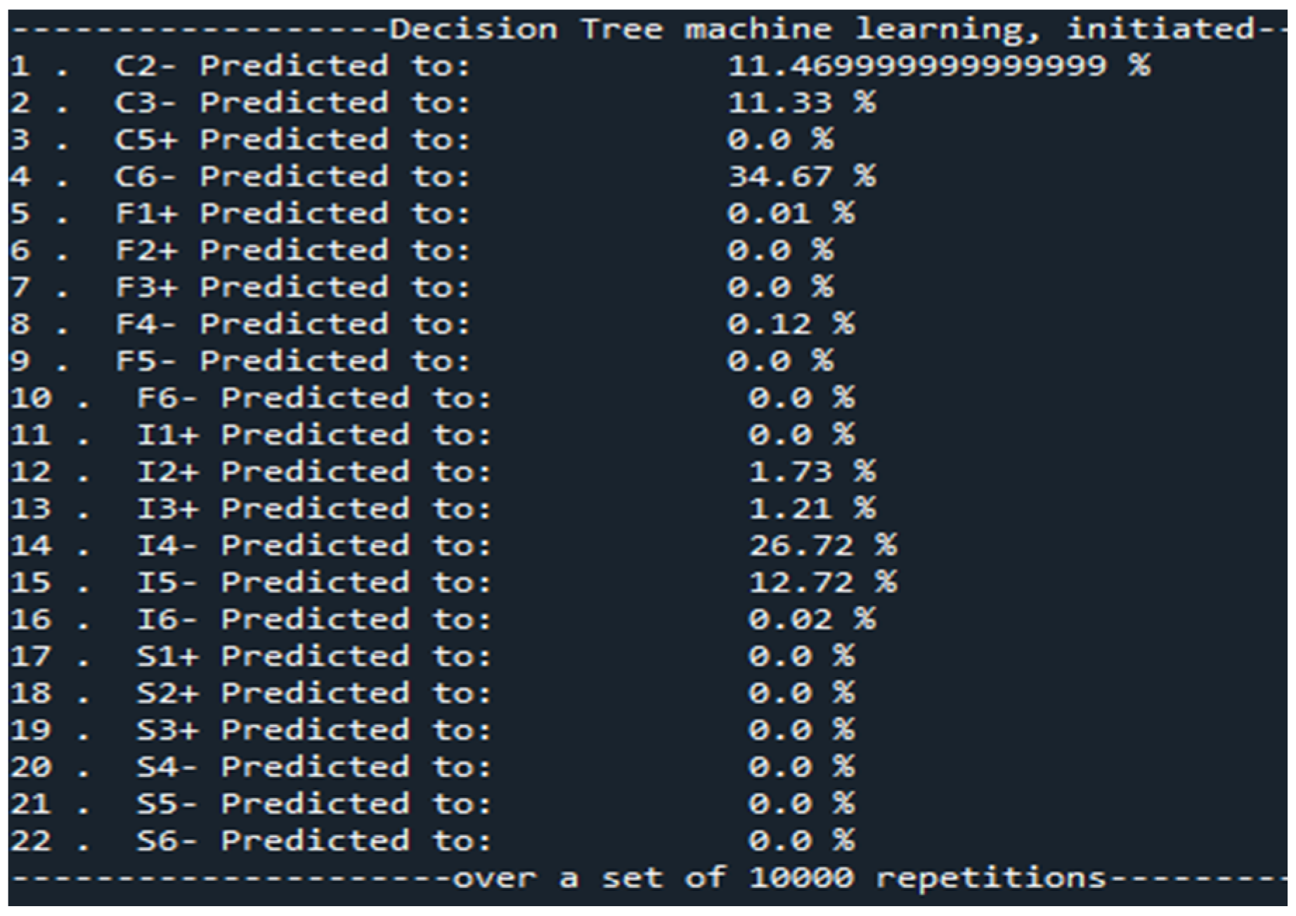
| Defect | Method | Classification |
|---|---|---|
| 4/14 | Visual | Corona (high confidence) |
| Combined test cells | Corona (90.6%) Surface (8%) Floating (0.6%) Cavity (0.73%) | |
| Segregated text cells | Negative corona test cell C6− (98.9%) | |
| Final | Corona | |
| 12/14 | Visual | Surface (low confidence) Noise (high confidence) |
| Combined test cells | Corona (56.0%) Surface (8.1%) Floating (0%) Cavity (31.6%) | |
| Segregated text cells | Positive corona test cell C5+ (6.01%) Positive floating test cell F2+ (31.7%) Negative cavity (internal) test cell I4− (26.32%) Negative cavity (internal) test cell I5− (34.58%) | |
| Final | Noise |
| Case | AC | DC (+) | DC (−) | ||||||
|---|---|---|---|---|---|---|---|---|---|
| Real | ACR1 | ACR2 | Real | DCR1 | DCR2 | Real | DCR1 | DCR2 | |
| 1 | Cavity | Cavity (98%) | Cavity (91%) | Surface | Cavity (48%) | Surface (99%) | Floating | Floating (84%) | Floating (97%) |
| 2 | Corona | Corona (99%) | Corona (99%) | Cavity | Cavity (67%) | Cavity (89%) | Surface | Noise | Surface (97%) |
| 3 | Floating | Floating (99%) | Floating (98%) | Corona | Corona (82%) | Corona (95%) | Noise | Noise | Corona (45%) |
| 4 | Noise | Floating (46%) | Noise (100%) | Floating | Floating (83%) | Floating (95%) | Corona | Corona (91%) | Corona (97%) |
| 5 | Surface | Surface (90%) | Surface (100%) | Cavity | Cavity (83%) | Cavity (99%) | Floating | Floating (84%) | Floating (98%) |
| 6 | Floating | Floating (97%) | Floating (84%) | Noise | Noise | Noise (81%) | Cavity | Cavity (65%) | Cavity (99%) |
| 7 | Corona | Surface (61%) | Corona (100%) | Surface | Surface (57%) | Surface (79%) | Surface | Noise | Surface (95%) |
| 8 | Cavity | Cavity (99%) | Cavity (100%) | Floating | Floating (87%) | Floating (95%) | Cavity | Cavity (83%) | Cavity (98%) |
| 9 | Surface | Surface (96%) | Surface (100%) | Corona | Corona (82%) | Corona (100%) | Corona | Corona (78%) | Corona (100%) |
| 10 | Cavity | Cavity (99%) | Cavity (100%) | Surface | Cavity (63%) | Surface (94%) | Floating | Floating (78%) | Floating (78%) |
| 11 | Noise | Noise (49%) | Noise (100%) | Noise | Noise | Noise (97%) | Cavity | Cavity (67%) | Cavity (99%) |
| 12 | Corona | Corona (98%) | Corona (97%) | Cavity | Cavity (68%) | Cavity (98%) | Noise | Noise | Noise (72%) |
| 13 | Surface | Cavity (54%) | Surface (100%) | Corona | Corona (78%) | Corona (98%) | Corona | Corona (86%) | Corona (100%) |
| 14 | Floating | Floating (100%) | Floating (99%) | Floating | Floating (100%) | Floating (98%) | Surface | Noise | Surface (94%) |
| AC Cases | Clustering Tool | Corona | Floating | Surface | Cavity | Noise #1 | Noise #2 |
| 1 | C1 | 49% | 100% | 100% | |||
| 2 | 31% | 99% | 100% | ||||
| 3 | 46% | 63% | 97% | ||||
| 4 | 80% | 74% | 100% | ||||
| 5 | No detected | 99% | 100% | ||||
| 6 | 48% | −96% Floating | −100% Surface | 99% | |||
| 7 | 100% | 99% | 99% | ||||
| 8 | 100% | Floating 85% | 100% | ||||
| 9 | 90% | 90% | 100% | ||||
| 10 | No detected | 99% | 99% | ||||
| 11 | 99% | No detected | 99% | ||||
| 12 | 99% | 97% | 99% | ||||
| Mean | 68.7% | 42.3% | 97.7% | 77.2% | 13.0% | 82.8% | 99.3% |
| 1 | C2 | No detected | 100% | 100% | |||
| 2 | 99% | 100% | 100% | ||||
| 3 | 100% | 100% | 100% | ||||
| 4 | No detected | 61% | 100% | ||||
| 5 | 100% | 100% | 99% | ||||
| 6 | 99% | 98% | 100% | ||||
| 7 | 100% | 100% | 100% | ||||
| 8 | 100% | 100% | 100% | ||||
| 9 | 100% | 100% | 97% | ||||
| 10 | 100% | 100% | 100% | ||||
| 11 | 100% | 100% | 95% | ||||
| 12 | 100% | 100% | 99% | ||||
| Mean | 93.0% | 66.3% | 100.0% | 93.5% | 99.7% | 99.2% | 99.2% |
| DC Cases | Clustering Tool | Corona | Floating | Surface | Cavity | Noise #1 | Noise #2 |
| DC (+) | C1 | 90% | 79% | 68% | 70% | ||
| DC (−) | 84% | 98% | 92% | 73% | |||
| Mean | 83.8% | 90.0% | 84.0% | 79.0% | 98.0% | 80.0% | 71.5% |
| DC (+) | C2 | 93% | 81% | 81% | 96% | ||
| DC (−) | 90% | 97% | 100% | 100% | |||
| Mean | 91.6% | 93.0% | 90.0% | 81.0% | 97.0% | 90.5% | 98.0% |
| Location Error (m) or (%) | |||||||
|---|---|---|---|---|---|---|---|
| Distance to T1 (m) | L1 | L2 | L3 | L4 | L5 | Max | |
| C | 24 m | −1.0 m | 1.0 m | −0.7 m | +1.1 m | −1.0 m | +1.1 m |
| A | 92 m | −0.43% | 0.00% | 0.19% | 1.63% | 0.05% | 1.63% |
| B | 117 m | 0.51% | 0.00% | 0.06% | 1.20% | 0.27% | 1.20% |
| Max ABS (ε) (m) | 1.0 m | 1.0 m | 0.7 m | 1.1 m | 1.0 m | 1.1 m | |
| Max ABS (ε) (%) | 0.51% | 0.00% | 0.20% | 1.60% | 0.30% | 1.63% | |
Disclaimer/Publisher’s Note: The statements, opinions and data contained in all publications are solely those of the individual author(s) and contributor(s) and not of MDPI and/or the editor(s). MDPI and/or the editor(s) disclaim responsibility for any injury to people or property resulting from any ideas, methods, instructions or products referred to in the content. |
© 2023 by the authors. Licensee MDPI, Basel, Switzerland. This article is an open access article distributed under the terms and conditions of the Creative Commons Attribution (CC BY) license (https://creativecommons.org/licenses/by/4.0/).
Share and Cite
Vera, C.; Garnacho, F.; Klüss, J.; Mier, C.; Álvarez, F.; Lahti, K.; Khamlichi, A.; Elg, A.-P.; Rodrigo Mor, A.; Arcones, E.; et al. Validation of a Qualification Procedure Applied to the Verification of Partial Discharge Analysers Used for HVDC or HVAC Networks. Appl. Sci. 2023, 13, 8214. https://doi.org/10.3390/app13148214
Vera C, Garnacho F, Klüss J, Mier C, Álvarez F, Lahti K, Khamlichi A, Elg A-P, Rodrigo Mor A, Arcones E, et al. Validation of a Qualification Procedure Applied to the Verification of Partial Discharge Analysers Used for HVDC or HVAC Networks. Applied Sciences. 2023; 13(14):8214. https://doi.org/10.3390/app13148214
Chicago/Turabian StyleVera, Carlos, Fernando Garnacho, Joni Klüss, Christian Mier, Fernando Álvarez, Kari Lahti, Abderrahim Khamlichi, Alf-Peter Elg, Armando Rodrigo Mor, Eduardo Arcones, and et al. 2023. "Validation of a Qualification Procedure Applied to the Verification of Partial Discharge Analysers Used for HVDC or HVAC Networks" Applied Sciences 13, no. 14: 8214. https://doi.org/10.3390/app13148214