On a Novel Approach to Correcting Temperature Dependencies in Magnetic Observatory Data

Abstract

High-quality geomagnetic measurements are widely used in both fundamental research of the magnetic field and numerous industrial applications. However, vector data measured by fluxgate sensors show a dependency on temperature due to sensitive coil core material and components of the sensor electronics. Here, we propose a new method for detecting and eliminating temperature dependence in magnetic observatory data. The method is designed to correct temperature drifts in variation vector magnetometer measurements when preparing quasi-definitive data according to an INTERMAGNET standard. A special feature of the method is the semi-automatic adjustment of localization intervals for temperature correction, which prevents boundary jumps and discontinuities in the course of sequential data processing over long intervals. The conservative nature of the approach implies the minimization of the original data amount subjected to correction. The described method is successfully applied in the routine monthly preparation of quasi-definitive data of the Saint Petersburg Observatory (IAGA-code SPG) and can be efficiently introduced at other magnetic observatories worldwide.

1. Introduction

The study of the nature of the Earth’s magnetic field (EMF) and the development of mathematical models to describe it are inseparable from improvements in methods for measuring and processing geomagnetic data. Despite a constant increase in the quantity and quality of measurements performed by research satellites in near-Earth space, ground-based continuous magnetic field measurements are still the most accurate and long-term series of observations of secular changes in the EMF [1,2]. The organization of the first magnetic observatories goes back to Carl Friedrich Gauss, who, as the founder of the EMF modelling method, realized the need for continuous observations of the EMF in specially equipped magnetic observatories. A major step towards building a global observation network was the International Geophysical Year (IGY), during which more than 1000 magnetic observatories were launched around the world [3]. The system of World Data Centers established during the IGY became the prototype of modern data repositories and anticipated the idea of distributed storage and exchange of scientific information [4]. The growing scientific and applied importance of high precision geomagnetic observations led to the foundation of the INTERMAGNET international network of magnetic observatories in 1991, which now includes about 130 observatories worldwide [1]. One of the main aims of the network was to ensure the high reliability of the accumulated geomagnetic data achieved by introducing new methods of measurement quality control, multistep reconciliation, and supplementing measurements with metadata. Since the formation of INTERMAGNET, the quality criteria for the network’s observation data [5] have become the de facto standard for use in modelling the Earth’s main magnetic field [6]. Highly accurate models are essential for both fundamental research in geophysics and space physics, as well as applications such as global satellite navigation [7], support for directional drilling [8,9,10], and many others. In order to achieve the required accuracy of observations, magnetic observatories are placed in locations free of local magnetic anomalies and away from sources of electromagnetic noise, such as roads, railways, and power lines.

The main measuring instrument of the magnetic observatory is a vector three-component magnetometer (variometer), which allows to measure variations of the total magnetic induction vector B. Obtaining the vector B total components from the variometer data is done by adding baseline values to the variations [11,12,13]. Observatories calculate baseline values based on absolute measurements, which are performed manually 1–2 times per week. One known disadvantage of the variometer is the temperature drift of the readings [14,15]. The temperature dependencies of a fluxgate sensor are often caused by temperature-dependent variations in the magnetic susceptibility of the material from which the coil cores are made. In addition, the temperature-dependent components of the sensor electronics also contribute to temperature drifts [16,17]. In order to reduce the drift effect, variometers are installed in thermostatically controlled pavilions that maintain the daily variation in sensor temperature at 1–2 °C. Such stability is difficult to achieve over the entire calendar year due to the dramatic summer and winter temperature variations. Magnetic observatories located in sharply continental climates are affected by annual variations of outdoor temperatures from −40 °C to +30 °C. Maintaining a stable sensor temperature in such conditions becomes problematic, especially due to the limited power supply in areas of distant observatories. Absolute measurements allow correcting temperature distortions on seasonal or monthly scales, while correcting daily or weekly scale distortions is a non-trivial task when preparing the definitive data [18,19].

According to INTERMAGNET, quasi-definitive data are processed geomagnetic data with no difference of more than 5 nT from definitive data of the given observatory [5]. In contrast to definitive data, which become available to the scientific community more than one year after the measurement, quasi-definitive data are produced within a one month delay [20]. Such data are extremely important for updating magnetic field models on a timely basis and calibration of satellite observations [21]. This paper proposes a new method of temperature correction tested in the preparation of quasi-definitive data of the INTERMAGNET Saint Petersburg Observatory (IAGA code SPG) [22,23,24]. In addition to temperature correction, the full data processing cycle also involves the removal of jumps and spikes from the magnetometer recordings [25]. However, the corresponding algorithms are out of the scope of the present paper.

2. Existing Approaches to Assessing the Quality of Observatory Data

In the manual for long-term magnetic observations [9], temperature correction of data is one of the stages of processing component variations recorded at observatories. In [16], it was experimentally shown that the temperature coefficient of the sensor depends not only on the physical principle of the magnetic field measurement, but also on the variometer design. In addition, the temperature dependence of the electronic components of the signal amplifiers and analog-to-digital converters can have a significant effect on the measurements. All these factors lead to temperature drifts of the vector variometers comparable to the required EMF measurement accuracy for building main field models. In order to control the long-term stability of variometer readings, magnetic observatories continuously record the modulus of the total EMF vector using proton- or Overhauser-type scalar magnetometers [26], which are least affected by temperature. A key indicator of the quality of magnetic observatory measurements is the difference between the full vector modulus calculated from variometer data F(v) and the full vector modulus measured by a scalar magnetometer F(s):

$$G=F\left(v\right)-F\left(s\right).$$

(1)

This value is called deltaF (G record), and it has been provided by INTERMAGNET observatories along with definitive data sets since 2009 [5]. Ideally, G values are in the range of −0.5 to 0.5 nT during periods of low geomagnetic activity, but can reach ±1–2 nT during periods of strong geomagnetic disturbances.

Since modern variometers are not capable of measuring the full values of the EMF components with a sufficient absolute accuracy [27], regular absolute measurements, supplementing the variations with baseline values, are an integral part of the observatory operation. Absolute measurements are made manually with a declinometer/inclinometer with a single-component fluxgate sensor (DIflux) fixed on the optical axis. The results are the values of the total components of the EMF vector at the time of the measurement t₀. The observed baseline values at time t₀ are:

$$X_b\left(t_0\right)={X\left(t_0\right)-X}_v\left(t_0\right),$$

(2)

$$Y_b\left(t_0\right)={Y\left(t_0\right)-Y}_v\left(t_0\right),$$

(3)

$$Z_b\left(t_0\right)={Z\left(t_0\right)-Z}_v\left(t_0\right),$$

(4)

where X_v, Y_v, and Z_v are variations of the EMF vector recorded by the variometer, with the addition of some offsets providing |G| values within 5 nT.

Thus, the baseline values are nothing more than variometer calibration corrections that eliminate long-term drifts. The stability of the baseline values and baseline-dependent G record throughout the year is a basic indicator of the quality of the data provided by the observatory [28,29].

Temperature correction in observatory data processing can be accomplished in two ways. The most obvious way to reduce the influence of temperature is to adjust the temperature of the sensor using active (heating) and passive (thermal insulation) temperature control. In one way or another, all INTERMAGNET magnetic observatories maintain a constant temperature inside the variation pavilion. However, this method does not allow for the complete elimination of temperature variations in sharply continental and arctic climates due to considerable temperature variations both on seasonal and diurnal scales. When processing variometer data, the temperature dependence can be eliminated automatically by adding daily baseline values to the variations. However, in some cases, this procedure fails due to an insufficient frequency of the baseline values compared to the temperature variation frequencies. In these cases, a local temperature correction becomes necessary.

3. Temperature Dependence in Data from the Saint Petersburg Observatory

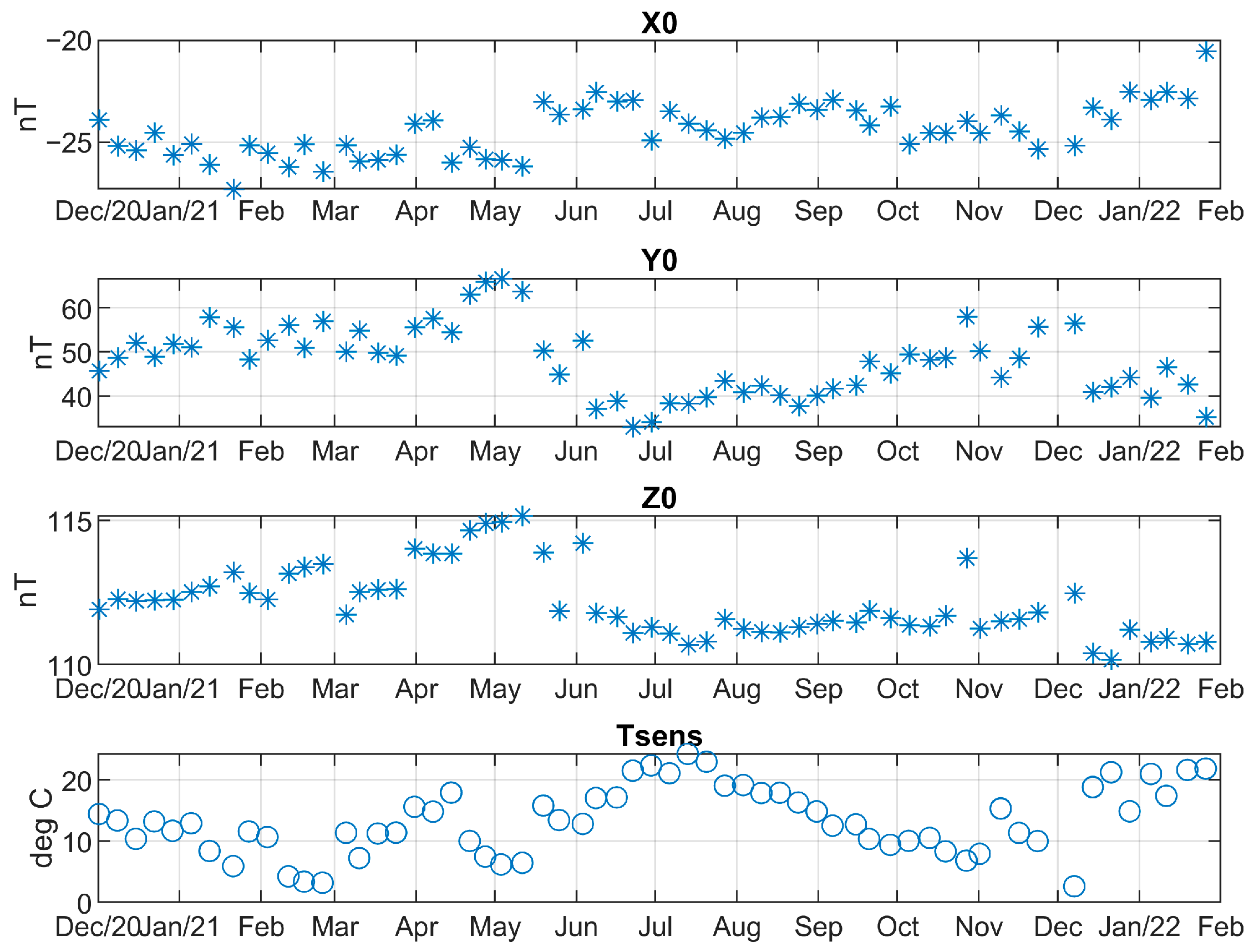
This section presents the most characteristic examples of the correlation between the G record and variometer sensor temperature, hereafter referred to as temperature dependencies, which one may observe in unadjusted 1-min data from the SPG observatory for various months of 2021. Figure 1 shows the observed variometer baseline values and the sensor temperature values at the time of the absolute measurements. Note that sharp temperature fluctuations in January–May and November–December 2021 led to jumps in the baseline values.

3.1. Typical Temperature Dependence in February 2021

Temperature dependencies most often occur when the behavior of the temperature plot during a month does not have a more or less constant downward or upward trend, but rather has a pronounced minimum or maximum—in other words, has a non-monotonous character during the month. In 2021, such a temperature trend is the most evident in February 2021, as shown in Figure 2.

In the example above, the G record clearly correlated with the temperature plot; as a result, a long-period component was added to the significant short-period G variations of small amplitude in this month. The situation looked especially critical at the beginning of the month when, due to the indicated effect, G values reached 0.6 nT, which exceeded the value of 0.5 nT adopted in observatory practice. The vertical lines in the figure mark the moments of fulfillment of absolute measurements. Still, applying these measurements through the observed baseline values did not lower G at the beginning of the month. The reason for this was that the daily baseline values were calculated by interpolating the observed baseline values, which were generated about once a week, with a smoothing spline. This function did not account for non-monotonous temperature variations between absolute measurements, which in turn led to undesirable distortions in the G graph.

3.2. Temperature Dependence in June 2021 when the Spline Breaks

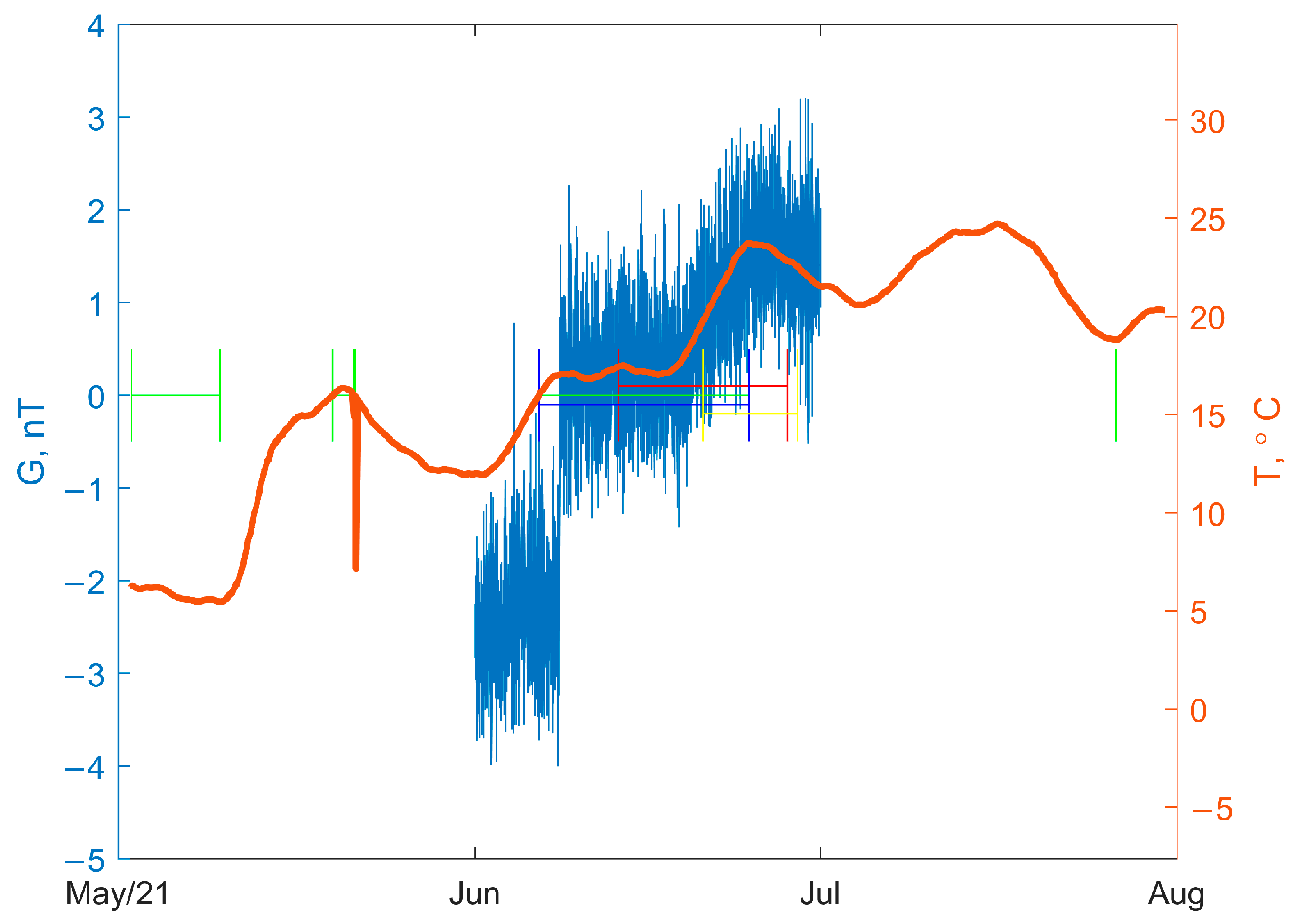
In early June 2021, there was a jump in the SPG data due to technical reasons, which led to a jump in the G plot as well. This plot, together with the variometer sensor temperature plot, are shown in Figure 3. The jumps in G in this case were usually corrected with a “break” of the baseline spline.

In this case, however, there was a visually evident similarity between G and the ascending segment of the temperature plot at the time of the data jump. Moreover, the absolute observations, marked by the second left vertical line in Figure 3, were made after the jump in the data. Taken together, this combination of factors led to the fact that, without the special temperature correction described in the next section, it was only possible to eliminate this jump by artificially inserting additional baseline values intraday. Such an approach was not stipulated by the INTERMAGNET standards, which required absolute measurements not more than once a day, so special justification should be provided when transmitting the definitive data to the INTERMAGNET. Such an insertion is also very time consuming to implement and, therefore, in general is highly undesirable. The need for a special temperature correction is also instigated due to the apparent temperature dependence G observed in the second half of June (Figure 3), during which the temperature plot, just as in February, had ascending and descending branches.

3.3. Temperature Dependence in November 2021 during a Magnetic Storm

On 4–5 November 2021, there was a fairly strong geomagnetic storm, which was reflected by the value of the planetary geomagnetic activity index Dst = −105 nT. Figure 4 shows the G and temperature plots of the variometer sensor of the SPG observatory during this storm. It is evident from the figure that the change in G values during the magnetic storm was caused by nothing other than an increase in temperature in the variation pavilion.

The INTERMAGNET requirements allowed a brief excess of the G threshold deviation of 0.5 nT during the geomagnetic storms. However, in this case, a segment with a peak amplitude of ~3 nT had a long duration (more than 4 days). It was caused by a local temperature change rather than by rapid magnetic field variations during a geomagnetic storm. Accordingly, such data without temperature correction were not reliable.

3.4. Temperature Dependence in December 2021 with an Abnormally Large Seasonal Temperature Change

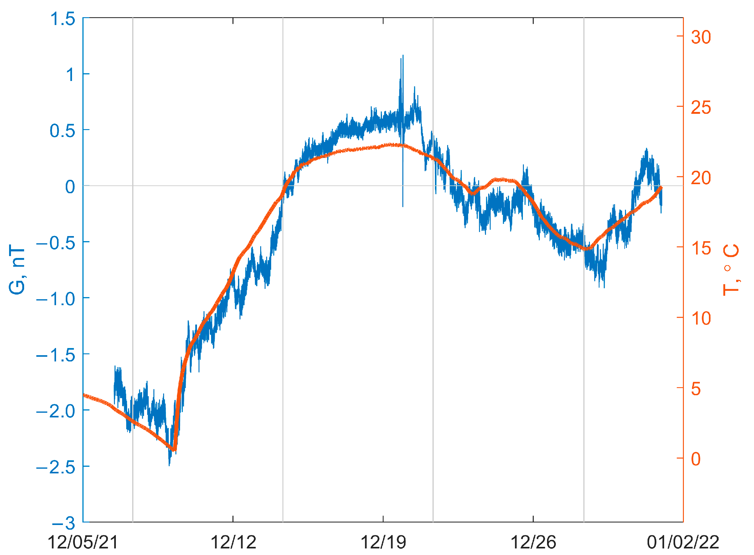
Throughout almost the entire November 2021, the outside temperature at the SPG observatory was fairly flat and positive between 3 and 5 °C. However, at the end of the month, it dropped first to −3 °C, and in early December even lower, reaching −14 and −17 °C on 5 and 6 December, respectively. Then, by 12–13 December the outside temperature returned to 0 °C and remained at this level until about 19 December, when it dropped again, and by the end of the month it was back to 0 °C again.

All this also affected the inside temperature measured at the variometer sensor, which is shown in Figure 5. In turn, this led to significant deviations in the G plot under reduced temperatures on 7 December 2021 and its high correlation with the temperature plot, despite making absolute observations on that day (first vertical line in Figure 5).

The temperature-dependent deviations of G from their usual permissible values during the first 12 days of December turned out to be too large, and the G plot itself was no longer a criterion of the quality of the obtained data, but a scaled and shifted temperature plot. As in the case of the data for February of the same year, adjusting the G plot by discarding the observed baseline values was unsuccessful due to the impossibility of accounting for intraday temperature variations. While the February 2021 G plot shown in Figure 2 was somehow acceptable as a criterion for the quality of the quasi-definitive data [21], the December 2021 G plot shown in Figure 5 cannot be evidence of the reliability of the obtained data.

4. Temperature Correction of Data

The examples discussed in the previous section clearly indicated the need for temperature correction of the obtained data. This section describes the proposed algorithm for such correction built in the course of routine processing of measurements from the Saint Petersburg Observatory. This algorithm includes four steps: (1) calculation of temperature correlations, (2) localization of temperature dependencies, (3) correction of variations, and (4) recalculation of baseline values. When determining the correlation between variometer readings and temperature, the G plots shown in Figure 2, Figure 3, Figure 4 and Figure 5 were not applicable because they depended on the baseline values, while the latter depended on the variometer readings, which just need to be corrected. Therefore, a centered G-mean(G) plot was considered instead of G to construct the correlation. The correlation was determined using the least square method, which resulted in two coefficients a and b, at which the graph a + bT(t), where T is temperature and t is time, lied closest to the graph G(t)-mean(G). The steps of the algorithm operation are illustrated below for each of the examples from the previous section.

The vector measurements of the magnetic field were performed with a 1 s sampling rate, so the data of the scalar magnetometer, which measures the magnetic field every 3 s, were piecewise linearly interpolated and resampled with a period of 1 s. The algorithm for the temperature drift reduction was designed for analyzing 1-s geomagnetic data supplemented with constant offsets. In this section, all presented plots are based on these data, in contrast to the previous section, which illustrated 1-min baseline corrected measurements.

4.1. Data for February 2021

To find the correlation coefficients a and b, we first manually specified time intervals at which approximations should be performed. Entering the interval for the correction manually enabled the minimization of the range of data correction, so fairly good data were not affected. The text file spt.txt was used to specify such intervals. Figure 2 showed that in this case, the correlation should be searched for almost the entire month. Therefore, for February 2021, the interval in the spt.txt file was set by the line

“2021-02-01 03:00:00; 2021-02-28 17:00:00”.

The resulting a + bT was shown in Figure 6 as an orange graph. Note that due to the G-mean(G) alignment, the graph of a + bT was also unbiased. The extension of the graph a + bT in both directions by 1 month was necessary for the second step of temperature correction—that is, the localization of temperature dependencies.

Why is localization done? Step 3 of the temperature correction implied the subtraction of the a + bT plot found in the previous step from the variometer readings. However, due to the complexity of temperature dependencies, the correlation of the G-mean(G) and a + bT plots was not universal—so, for example, the dependence found for February could no longer be applied even in March. Thus, this dependence was always local—i.e., applied to a fixed time interval. Accordingly, the values of a + bT would only be subtracted from the variometer readings within the time interval where the dependence was still valid. However, if the values at the ends of the interval were non-zero, then there would inevitably be discontinuities in the corrected readings at the boundaries when merging with data from adjacent measurement intervals. Localization meant defining time intervals for which two conditions were fulfilled: a unified temperature dependence was valid inside; a + bT took zero values at the boundaries. Such intervals were found programmatically. In Figure 6 they were marked with green; their ends corresponded to points of the a + bT transition through 0 (the algorithm marks other special fragments in green as well, which will be described later). Thus, correcting the variometer readings on the green interval in the central part of Figure 6 would not lead to data discontinuities on its boundaries.

A second text file spc.txt was used to specify all localization parameters and temperature dependencies required for the algorithm operation. For example, if the data of February 2021 were analyzed, the user entered the following line into the spc.txt file:

“a2021-02; 2021-02-01 00:00:00; 2021-03-01 00:00:00”.

In this line, the first letter “a” denoted the automatic localization mode; it was followed by the year and month for which the correction was performed, and after the semicolon it was followed by two dates, accurate to the second, corresponding approximately to the beginning and end of the segment of interest. The algorithm converted this string into the string

“a2021-02; 2021-02-08 21:48:00; 2021-02-26 03:00:00; −0.8665; 0.1621”.

In this line, the automatically defined start and end dates were the closest to the boundaries of the green segment in Figure 6. The automatically determined localization interval was indicated in blue in Figure 6. At the end of the line, there were the coefficients a and b of the temperature correlation determined in the first step.

Note that the automatically determined interval started from February 8. Thus, the fragment of the data for February 1–8, which was characterized by strong distortions in the G plot (see Figure 2) due to the temperature dependence of the obtained measurements, remained unaccounted. In order to account for it, the manual mode of setting temperature correction parameters was used. In this case, we took advantage of the fact that in January, the a + bT dependence character was close to that in February (Figure 6). By setting the correlation search interval equal to two months at once (1 January–1 March 2021), we determined the new correlation coefficients: a = −0.9195 and b = 0.1240. Concurrently, the right end of the green segment for February moved from 2021-02-26 03:00:00 to 2021-02-27 01:44:00. All the newly obtained information must be added to the spc.txt file as the line

“m2021-02; 2021-02-01 00:00:00; 2021-02-27 01:44:00; −0.9195; 0.1240”,

where “m” stands for the manual localization mode. The manually set localization interval started from 1 February and was shown by the yellow segment in Figure 6. When going over 1 February, the merging with the January data must be ensured. For this purpose, the temperature correction of the January data was performed with the unified correlation coefficients a = −0.9195 and b = 0.1240. As mentioned above, it was sufficient to correct only a fragment of the data starting from the last transition of a + bT through zero in January—i.e., for the interval from January 20 to February 1 (Figure 6).

Once the spc.txt file was generated, it was used directly for temperature correction, including the recalculation of component variations, observed and daily baseline values, and then G. The recalculation of variations at each time point t was done by including a VC(t) correction term into the standard calculation, which is derived as follows. If time moment t does not fall within the localization intervals presented in the spc.txt file, the variometer readings for that time moment are not corrected. For variometer readings falling in time into the localization interval i, the VC(t) is calculated by the formula

$$VC\left(t\right)=a_i+b_i{T}_t,$$

(5)

where a_i and b_i are the correlation coefficients for the localization interval i and T_t is the temperature at time t.

Then, the vector length from the variometer readings at time t is calculated:

$$VA\left(t\right)=\sqrt{Xv{\left(t\right)}^2+Yv{\left(t\right)}^2+Zv{\left(t\right)}^2.}$$

(6)

Finally, the values X_v(t), Y_v(t), and Z_v(t) of the variometer readings at time t are corrected using the formulas

$${Xv\left(t\right)}^{*}=Xv\left(t\right)\left(1-\frac{VC\left(t\right)}{VA\left(t\right)}\right),$$

(7)

$${Yv\left(t\right)}^{*}=Yv\left(t\right)\left(1-\frac{VC\left(t\right)}{VA\left(t\right)}\right),$$

(8)

$${Zv\left(t\right)}^{*}=Zv\left(t\right)\left(1-\frac{VC\left(t\right)}{VA\left(t\right)}\right).$$

(9)

The updated values X_v(t)^∗, Y_v(t)^∗, and Z_v(t)^∗ are then used instead of the values X_v(t), Y_v(t), and Z_v(t) in the standard calculations of the observed and daily baseline values and G.

Figure 7 shows, in blue, the plot of G for February 2021 calculated from the corrected variometer readings taking into account the original baseline values. It still had a slight drift in the first half of the month, which was eliminated by recalculating the observed baseline values (in this case, from the absolute measurements made on February 3 and 11). Graph G for February 2021 derived from the fully corrected data is shown in orange in Figure 7.

4.2. Data for June 2021

The G-mean(G) plot for June 2021 after correcting May data is shown in Figure 8. The difficulty with this case was that this graph contained a jump on 8 June, so only its left or right side could be corrected using a single interval. However, it should be noted that the graph a + bT from mid-May crossed zero on May 16 and June 8, precisely in the vicinity of the jump in the data. Thus, the 1–8 June data correction was successfully implemented in the course of the temperature correction of the May 2021 data, using an extended localization interval up to the June break point. The result is the constancy of the G-mean(G) plot for 1–8 June in Figure 8 (here, the plot was still biased from zero, as centered G variations with constant offsets were considered).

The problem thus boiled down to adjusting the data in June after the jump. From 8 to 13 June, the temperature was kept constant (see the scale on the right in Figure 8), which did not require a temperature correction. The temperature correction from 13 June 2021 was complicated by the fact that in the second half of June, the graph a + bT (Figure 8) went upwards, deviating strongly from zero, and remained in this zone throughout July 2021. Consequently, in this case, it was not possible to match the temperature corrections in June and July by analogy with the mechanism described above for the January–February data.

This situation was among those in which the localization interval cannot be bound to the points of the a + bT transition through zero. In this case, the algorithm provided the following procedure. At the end of the localization interval, where such binding was missing, an additional extension was formed, on which a smooth merging with the neighboring data fragment was further performed. The overall localization interval was thereby split into the following segments: the left-hand extension LS (if merging was required on the left), the inner segment IS, and the right-hand extension RS (if merging was required on the right). For proper merging, the inner boundary of the extension (i.e., the right end of the LS segment and/or the left end of the RS segment) must correspond to the point of a local extremum on the a + bT function. All such extrema located outside the area of the a + bT transition through zero were automatically marked by the algorithm. In Figure 6 and Figure 8, they corresponded to the ends of the green segments. The outer boundary of extension (i.e., the left end of the LS segment and/or the right end of the RS segment) where the correction should reduce to zero was determined by the nearest date of the absolute measurement. Within the IS segment, the correction was carried out as usual. On extension, the merging was performed by reducing the correction term to zero linearly (the formula is given for the RS segment):

$$VC\left(t\right)=VC\left(t\right)\left(1-\frac{t-t_0}{t_1-t_0} \right),$$

(10)

where VC(t) is the correction term at time t; t₀, t₁ are the left and right boundaries of the RS segment, respectively (for the LS segment, the calculations were similar).

As discussed above, in our case, such a merging was only required on the right side. In Figure 8, the most appropriate boundaries for the IS segment were defined by the central green interval—its left end coincided with the a + bT zero crossing, while the right end corresponded to the local extreme of a + bT (2021-06-21 19:40:00), being the left boundary of the RS segment. The right boundary of the RS segment corresponded to the right end of the red interval (2021-06-29 00:00:00).

When calculating the correlation coefficients on the IS segment, the following values were obtained by the algorithm: a = −3.9925 and b = 0.2019. Their previous values corresponding to the a + bT plot in Figure 8 were a = −3.385 and b = 0.2119. As a result, the graph a + bT shifted down by δa = −3.385 + 3.9925 = 0.6075 relative to its position in Figure 8. The coefficient b also changed insignificantly by δb = 0.2119 − 0.2019 = 0.01. As a result, the left boundary of the IS segment corresponding to the transition through 0 of the new graph a + bT shifted to the right at the time 2021-06-20 19:40:00. The obtained correlation parameters and the localization interval were manually set in the spc.txt file as follows:

“m2021-06;2021-06-20 19:40:00; 2021-06-21 19:40:00 * 2021-06-29 00:00:00; −3.9925; 0.2019”.

Here, the two time stamps separated by an asterisk denoted the RS segment boundaries.

So, with this line assignment in the spc.txt file for June 2021, the temperature correction was performed only on the rather short localization interval depicted in Figure 8 by the yellow segment. After the jump in the G-mean(G) plot and outside this interval, the temperature correction was performed successfully by a daily smoothed baseline.

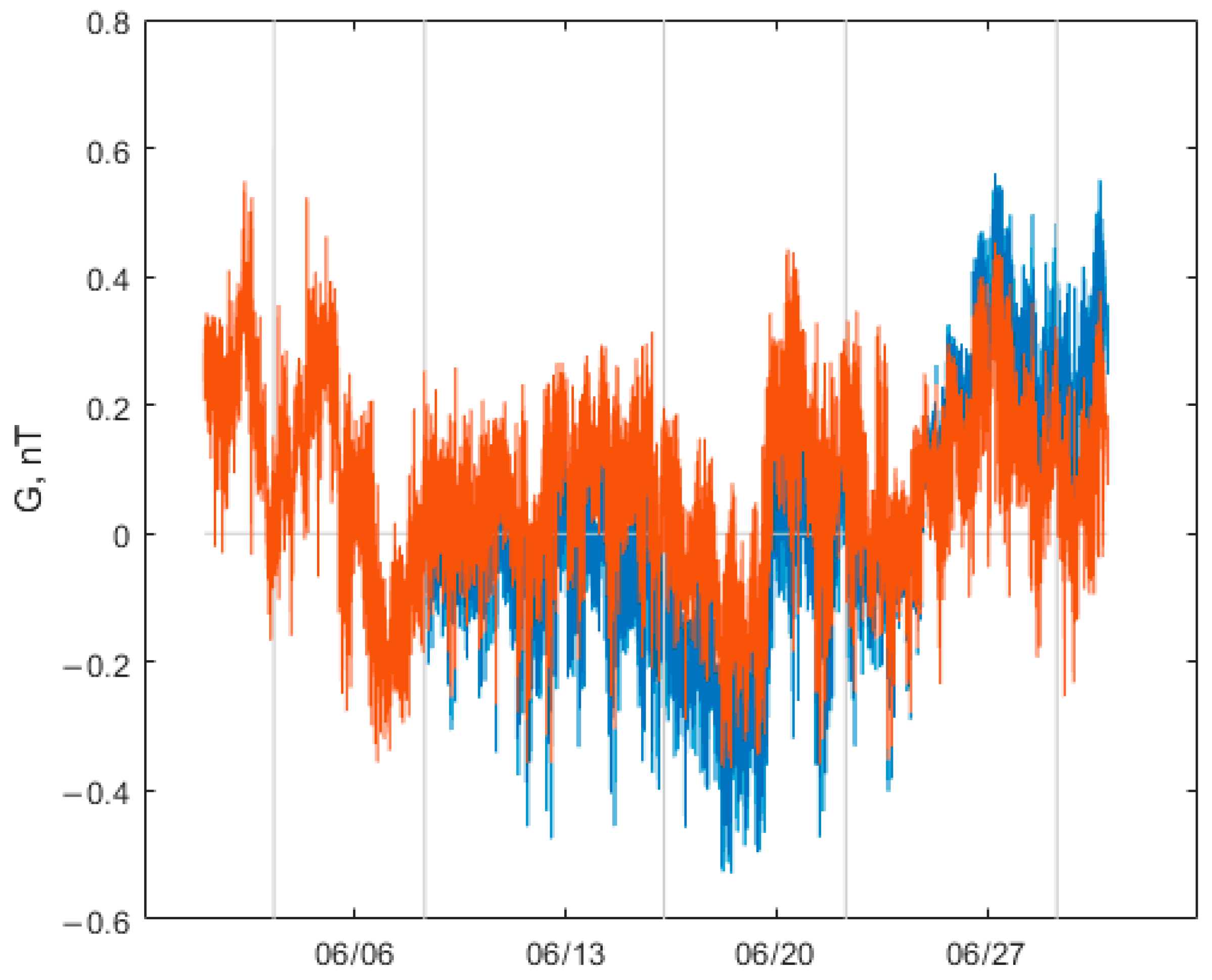
Figure 9 shows the G graph based on the adjusted variations, but original baseline values, in June 2021 (blue color). As in February, some biases in its behavior still remained. These were corrected by computing the new observed baseline values, here referring to the absolute measurements of 16, 22, and 29 June 2021. The final graph G, based on the fully recalculated data for June 2021, is shown in orange in Figure 9.

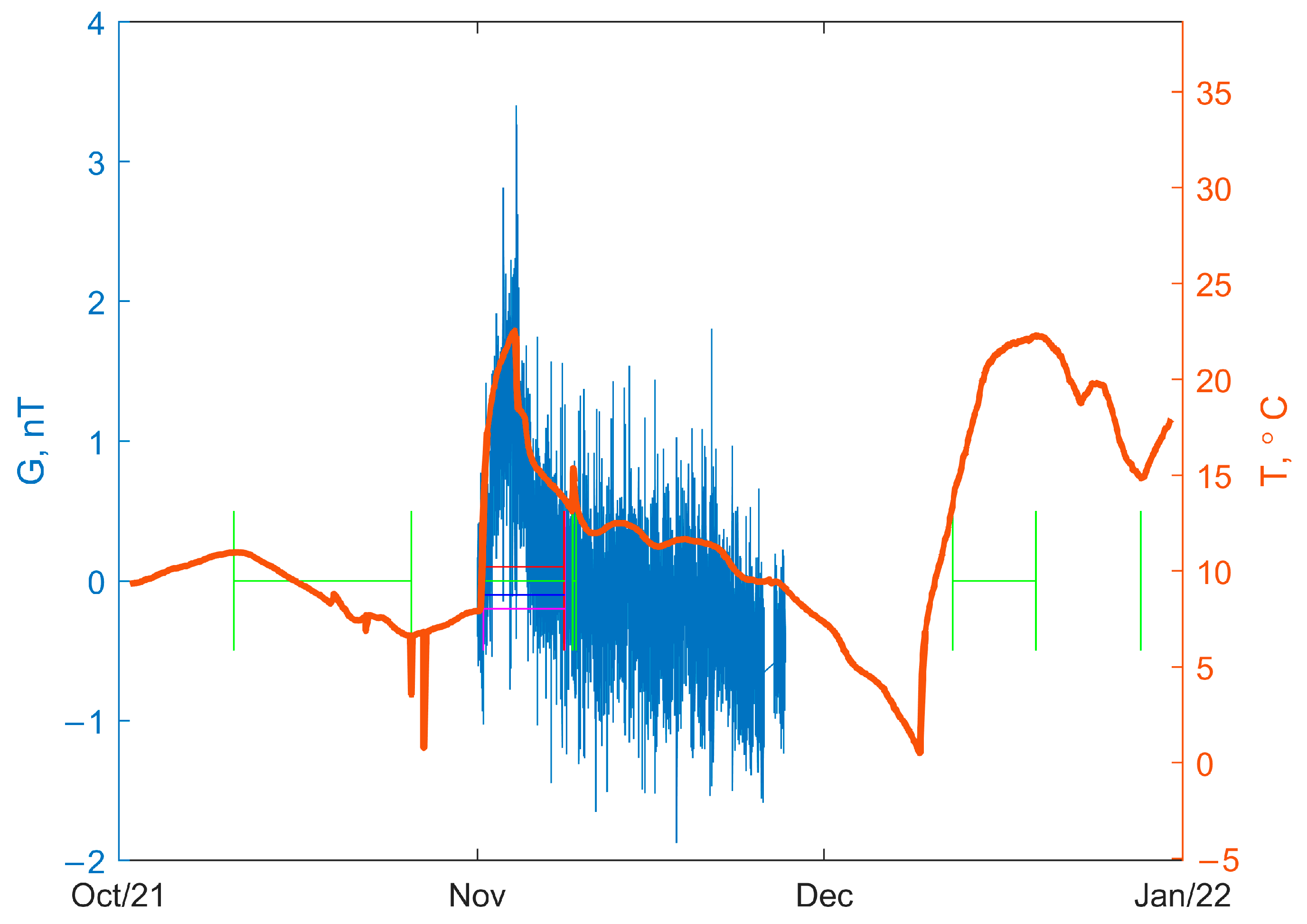
4.3. Data for November 2021

The G-mean(G) plot for November 2021 is shown in Figure 10. It is characterized by a bell-shaped form at the beginning of the month during a magnetic storm. The graph then tends to decrease towards the end of the month, which correlates well with temperature. Typically, such a constant trend is eliminated by the standard application of a daily smoothed baseline. However, the graph G, without the temperature correction shown earlier in Figure 4, demonstrated that the trend is not fully eliminated by the standard procedure, so a temperature correction at the end of the month is still desirable.

From the end of November, the a + bT graph went into a negative-value area, and by December 9, it rapidly returned to zero. Extending the November localization interval to this date, similar to that of May 2021, would result in a jump at the starting point of December’s temperature correction. If one moved in the opposite direction, from December to November, the graph of a + bT somehow crossed zero during November. Thus, a more accurate removal of a downward slope of the G-mean(G) graph at the November–December transition would be provided while correcting the December data over the localization interval extended to the left.

Thus, the temperature correction in November was just about the elimination of the bell-shaped segment of the G-mean(G) graph at the start of the month. For that, we first specified the reference interval in the spt.txt file for November 2021 as

“2021-11-01 11:15:00; 2021-11-08 12:00:00”.

In Figure 10, this reference interval was shown as a red segment; its choice corresponded to the best approximation of the G-mean(G) bell shape by the correlated temperature graph a + bT. Afterwards, we set in the spc.txt file the automatic mode and the approximate position of the boundaries of the localization interval, for example, by simply transferring the reference interval from the spt.txt file:

“a2021-11; 2021-11-01 11:15:00; 2021-11-08 12:00:00”.

As a result of the algorithm execution, this string is converted into a string

“a2021-11; 2021-11-01 13:36:00; 2021-11-08 15:37:00; −2.1844; 0.1600”,

which contains the defined exact localization interval and the correlation coefficients. In Figure 9, this interval was depicted, as in the previous examples, by a blue segment. In this case, its ends exactly coincided with the ends of the centrally located green segment, denoting the points of transition of the graph a + bT through 0 before and after the “bell” in the graph G-mean(G).

The G plot for November 2021 after the temperature correction of the variation data is shown in blue in Figure 11. Due to the use of the former baseline values, the graph contains a clear artificial positive trend in the range of absolute measurements on 9 November. As before, its elimination was provided by recalculating the baseline values using the corrected variation data. The final graph G for November 2021 is shown in orange.

4.4. Data for December 2021

The impact of temperature on the behavior of the G-mean(G) graph is most visible in December 2021 (Figure 12). However, in terms of temperature correction, this case turned out to be fairly straightforward.

The G-mean(G) graph correlated well with the temperature graph throughout the month, so in the spt.txt file, the reference interval is set to a whole month:

“2021-12-01 00:00:00; 2022-01-01 00:00:00”.

As usual, this interval was indicated in Figure 12 by a red segment, and the green segments marked possible correction interval limits. Obviously, for December 2021, the automatic mode for the localization interval selection was well suited, as it ensured that the a + bT graph crossed zero at its ends. Thus, the approximate beginning of the interval could be the vicinity of the right-hand boundary of the green segment located in Figure 12 at the beginning of November after the bay of the a + bT graph. The approximate end of the interval could be the vicinity of the left-hand boundary of the green segment going from December 2021 to January 2022. As a result of the algorithm execution, the corresponding line in the spc.txt file will be overwritten as

“a2021-12; 2021-11-05 14:20:00; 2021-12-29 09:21:00; −2.1600; 0.1346”.

The automatically chosen localization interval in Figure 12 was shown in blue and ran from 5 November to 29 December 2021, covering almost two months. Notably, it intersected with the localization interval for November 2021 (see previous sub-section) from 5–8 November, so at the intersection, the correction procedure accounted for both intervals. For variometer readings falling within this intersection, the VC(t) correction term is

$$VC\left(t\right)=\sum _i{(a}_i+b_i{T}_t),$$

(11)

where i is the ordinal numbers of the overlapping localization intervals.

Figure 13 shows plots G for December 2021 derived from the temperature adjusted variations only (in blue), and the recalculated baseline values (in orange).

5. Discussion

In the previous sections, we demonstrated applications of the temperature correction algorithm using the most typical examples revealed in February, June, November, and December 2021. The first and second examples demonstrated the algorithm capabilities under significant temperature variations, which one may observe regularly. The third and fourth examples demonstrated the difficulties of data correction under increased geomagnetic activity conditions and sharp extreme temperature fluctuations. In total, a temperature correction procedure was performed in 10 out of 12 months in 2021, all except August and October.

The algorithm execution was comprised of the following stages:

1. Calculation of the linear regression coefficients for the temperature recordings to fit the G plot and markup of the raw data within the user-defined interval;

2. Specification of the data segment and mode for data correction by the user based on the markup results (stage 1);

3. Correction of the data according to the temperature coefficients (stage 1) and mode (stage 2), which guaranteed a smooth merging of the corrected data with the previously processed data segments. The application of the described algorithm in the course of preparation of quasi-definitive data of the Saint Petersburg Observatory enabled the prompt elimination of temperature driven distortions of the full EMF vector components. Such distortions included both local temperature drifts and jumps at daily boundaries associated with abrupt changes in temperature.

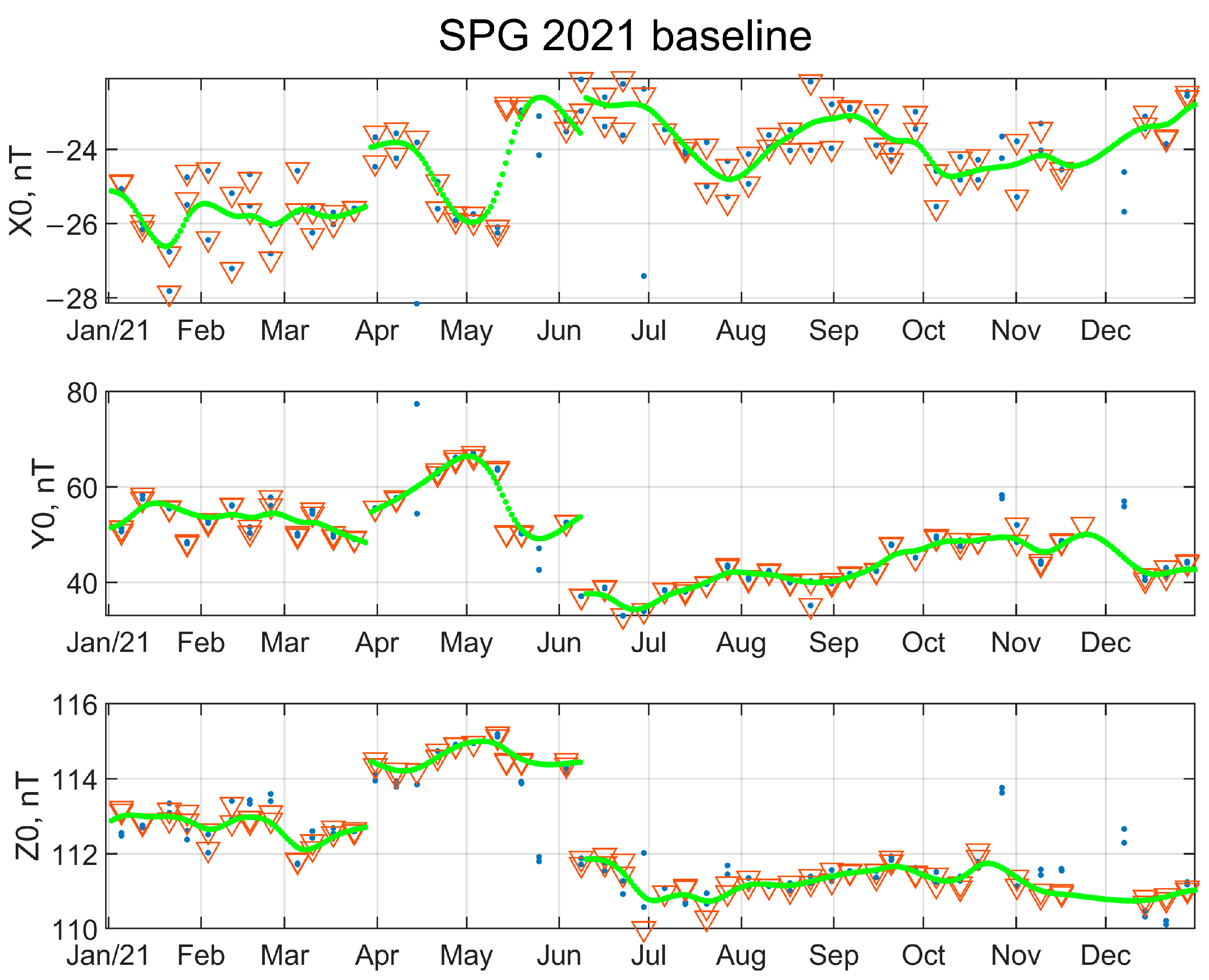
It should be noted that the described approach was based on the principle of minimal interference with the original data. Thus, temperature corrections affected less than 25% of the variation data in 2021, which entailed recalculation of only 10 observed baseline values out of 47. Figure 14 shows a comparative plot of the original baseline values marked by the blue dots and those corrected using the described algorithm (red triangles). The isolated points of the original baseline values are outliers due to measurement errors or instrumental effects. As seen from Figure 14, substantial corrections have mostly affected only the data intervals discussed in the article. The corrected data from the Saint Petersburg Observatory, together with data from the Klimovskaya Observatory [30,31], were used in [32] for detection of the most recent geomagnetic jerk, which indicated the efficiency of the proposed method and high reliability of the obtained data.

Correction of temperature-driven distortions in geomagnetic measurements is crucial in observatory practice, and the geomagnetic community makes efforts to tackle this problem [18,19]. However, a method proposed in [18] implied the correction of the yearly data set at the stage of definitive data production. Our approach was capable to correct data on a monthly basis, which makes quasi-definitive data available promptly. An approach reported in [19] was based on the comparison with other observatory data and required a dense enough network of observatories. Our method did not involve data from other observatories in any way, so it only crunched data from a single observatory under consideration.

Many other environmental observation instruments are subjected to temperature drifts, so it is a common problem in data quality control (e.g., [33,34]). However, the proposed method for the measurement correction was adapted to the combination of two sensors (fluxgate and Overhauser proton) specifically designed for magnetic observations and based on different physical principles. This combination enabled revealing distortions in each other’s data. Therefore, the method was barely applicable to correcting measurements from other type of sensors.

References

- Love, J.J.; Chulliat, A. An international network of magnetic observatories. Eos Trans. Am. Geophys. Union 2013, 94, 373–374. [Google Scholar] [CrossRef]
- Soloviev, A.A. Some challenges of geomagnetism addressed with the use of ground and satellite observations. Russ. Geol. Geophys. 2023, 45–60. [Google Scholar] [CrossRef]
- Lyubovtseva, Y.S.; Gvishiani, A.D.; Soloviev, A.A.; Samokhina, O.O.; Krasnoperov, R.I. Sixtieth anniversary of the International Geophysical Year (1957–2017)–contribution of the Soviet Union. Hist. Geo-Space Sci. 2020, 11, 157–171. [Google Scholar] [CrossRef]
- Korsmo, F.L. The Origins and Principles of the World Data Center System. Data Sci. J. 2009, 8, IGY55–IGY65. [Google Scholar] [CrossRef]
- St-Louis, B. INTERMAGNET Technical Reference Manual, version 5.0.0; INTERMAGNET Operations Committee and Executive Council: Ottawa, ON, Canada, 2020; p. 146. [Google Scholar]
- Alken, P.; Thébault, E.; Beggan, C.D.; Amit, H.; Aubert, J.; Baerenzung, J.; Bondar, T.N.; Brown, W.J.; Califf, S.; Chambodut, A.; et al. International Geomagnetic Reference Field: The thirteenth generation. Earth Planets Space 2021, 73, 49. [Google Scholar] [CrossRef]
- Petrie, E.J.; King, M.A.; Moore, P.; Lavallée, D.A. Higher-order ionospheric effects on the GPS reference frame and velocities. J. Geophys. Res. 2010, 115, 148–227. [Google Scholar] [CrossRef] [Green Version]
- Soloviev, A.A.; Sidorov, R.V.; Oshchenko, A.A.; Zaitsev, A.N. On the need for accurate monitoring of the geomagnetic field during directional drilling in the Russian Arctic, Izvestiya. Phys. Solid Earth 2022, 58, 420–434. [Google Scholar] [CrossRef]
- Gvishiani, A.D.; Lukianova, R.Y. Estimating the influence of geomagnetic disturbances on the trajectory of the directional drilling of deep wells in the Arctic region. Izv. Phys. Solid Earth 2018, 54, 554–564. [Google Scholar] [CrossRef]
- Gvishiani, A.D.; Lukianova, R.Y.; Soloviev, A.A. Geomagnetic field analysis and directional drilling accuracy problem in the Arctic region. Gorn. Zhurnal 2015, 10, 94–99. [Google Scholar] [CrossRef] [Green Version]
- Rasson, J.L. About Absolute Geomagnetic Measurements in the Observatory and in the Field; Publication Scientifique et Technique N 040; L’Institut Royal Metrologique de Belgique: Brussel, Belgium, 2005. [Google Scholar]
- Xin, C.J.; Shen, W.R.; Li, Q.H.; Tian, W.T. The comparison and analysis of the baseline values of null method and offset method. Seismol. Geomagn. Obs. Res. 2003, 24, 77–80. [Google Scholar]
- Zhang, S.Q.; Yang, D.M. Study on the stability and accuracy of baseline values measured during the calibrating time intervals. Data Sci. J. 2011, 10, IAGA19–IAGA24. [Google Scholar] [CrossRef]
- Primdahl, P. The fluxgate magnetometer. J. Phys. E Sci. Instrum. 1979, 12, 241–253. [Google Scholar] [CrossRef]
- Jankowski, J.; Sucksdorff, C. Guide for Magnetic Measurements and Observatory Practice; IAGA: Warsaw, Poland, 1996; pp. 225–232. [Google Scholar]
- Csontos, A.; Hegymegi, L.; Heilig, B. Temperature tests on modern magnetometers. Publ. Inst. Geophys. Pol. Acad. Sci. 2007, 99, 171–177. [Google Scholar]
- Ripka, P. Magnetic Sensors and Magnetometers, 2nd ed.; Artech House: Norwood, MA, USA, 2021; 416p, ISBN 1630817430/9781630817435. [Google Scholar]
- Janošek, M.; Butta, M.; Vlk, M.; Bayer, T. Improving Earth’s Magnetic Field Measurements by Numerical Corrections of Thermal Drifts and Man-Made Disturbances. J. Sens. 2018, 2018, 1804092. [Google Scholar] [CrossRef]
- He, Z.; Hu, X.; Teng, Y.; Zhang, X.; Shen, X. Data agreement analysis and correction of comparative geomagnetic vector observations. Earth Planets Space 2022, 74, 29. [Google Scholar] [CrossRef]
- Peltier, A.; Chulliat, A. On the feasibility of promptly producing quasi-definitive magnetic observatory data. Earth Planets Space 2010, 62, e5–e8. [Google Scholar] [CrossRef] [Green Version]
- Soloviev, A.A.; Peregoudov, D.V. Verification of the geomagnetic field models using historical satellite measurements obtained in 1964 and 1970. Earth Planets Space 2022, 74, 187. [Google Scholar] [CrossRef]
- Sidorov, R.V.; Soloviev, A.A.; Krasnoperov, R.I.; Kudin, D.V.; Grudnev, A.A.; Kopytenko, Y.A.; Kotikov, A.L.; Sergushin, P. Saint Petersburg magnetic observatory: From Voeikovo subdivision to INTERMAGNET certification. Geosci. Instrum. Methods Data Syst. 2017, 6, 473–485. [Google Scholar] [CrossRef] [Green Version]
- Soloviev, A.A.; Kopytenko, Y.A.; Kotikov, A.L.; Kudin, D.V.; Sidorov, R.V. 2017 Definitive Data from Geomagnetic Observatory Saint Petersburg (IAGA Code: SPG): Minute Values of X, Y, Z Components and Total Intensity F of the Earth’s Magnetic Field; ESDB Repository; GCRAS: Moscow, Russia, 2020. [Google Scholar] [CrossRef]
- Soloviev, A.A.; Kopytenko, Y.A.; Kotikov, A.L.; Kudin, D.V.; Sidorov, R.V.; Matveev, M.N. 2020 Definitive Data from Geomagnetic Observatory Saint Petersburg (IAGA Code: SPG): Minute Values of X, Y, Z Components and Total Intensity F of the Earth’s Magnetic Field; ESDB Repository; GCRAS: Moscow, Russia, 2021. [Google Scholar] [CrossRef]
- Kudin, D.V.; Soloviev, A.A.; Sidorov, R.V.; Starostenko, V.I.; Sumaruk, Y.P.; Legostaeva, O.V. Advanced production of quasi- definitive magnetic observatory data of the INTERMAGNET standard. Geomagn. Aeron. 2021, 61, 54–67. [Google Scholar] [CrossRef]
- Khomutov, S.Y.; Kusonsky, O.A.; Rasson, J.L.; Sapunov, V.A. The Using of the Absolute Overhauser Magnetometers POS-1 in Observatory Practice: The Results of the First 2.5 Years. In Proceedings of the XI IAGA Workshop on Geomagnetic Observatory Instruments, Data Acquisition and Processing: Book of Abstracts, Kakioka, Japan, 9–12 November 2004. [Google Scholar]
- Korepanov, V.; Marusenkov, A. Fluxgate magnetometers design peculiarities. Surv. Geophys. 2012, 33, 1059–1079. [Google Scholar] [CrossRef] [Green Version]
- Lesur, V.; Heumez, B.; Telali, A.; Lalanne, X.; Soloviev, A.A. Estimating error statistics for Chambon-la-Forêt observatory definitive data. Ann. Geophys. 2017, 35, 939–952. [Google Scholar] [CrossRef] [Green Version]
- Soloviev, A.A.; Lesur, V.; Kudin, D.V. On the feasibility of routine baseline improvement in processing of geomagnetic observatory data. Earth Planets Space 2018, 70, 16. [Google Scholar] [CrossRef]
- Soloviev, A.A.; Dobrovolsky, M.N.; Kudin, D.V.; Sidorov, R.V. Minute Values of X, Y, Z Components and Total Intensity F of the Earth’s Magnetic Field from Geomagnetic Observatory Klimovskaya (IAGA Code: KLI); ESDB Repository; Geophysical Center of the Russian Academy of Sciences: Moscow, Russia, 2015. [Google Scholar] [CrossRef]
- Soloviev, A.A.; Sidorov, R.V.; Krasnoperov, R.I.; Grudnev, A.A.; Khokhlov, A.V. Klimovskaya: A New Geomagnetic Observatory. Geomagn. Aeron. 2016, 56, 342–354. [Google Scholar] [CrossRef]
- Soloviev, A.A.; Kudin, D.V.; Sidorov, R.V.; Kotikov, A.L. Detection of the 2020 Geomagnetic Jerk Using near Real-Time Data from the “St. Petersburg” and “Klimovskaya” Magnetic Observatories. Dokl. Earth Sci. 2022, 507, 925–929. [Google Scholar] [CrossRef]
- Owens, D.; Abeysirigunawardena, D.; Biffard, B.; Chen, Y.; Conley, P.; Jenkyns, R.; Kerschtien, S.; Lavallee, T.; MacArthur, M.; Mousseau, J.; et al. The Oceans 2.0/3.0 Data Management and Archival System. Front. Mar. Sci. 2022, 9, 806452. [Google Scholar] [CrossRef]
- Chatzievangelou, D.; Aguzzi, J.; Scherwath, M.; Thomsen, L. Quality Control and Pre-Analysis Treatment of the Environmental Datasets Collected by an Internet Operated Deep-Sea Crawler during Its Entire 7-Year Long Deployment (2009–2016). Sensors 2020, 20, 2991. [Google Scholar] [CrossRef]
Figure 1.
Observed baseline values of the three components (top three plots) and variometer sensor temperature (hourly means, bottom plot) at the time of absolute measurements at the Saint Petersburg Observatory (SPG) in 2021.
Figure 2.
Plots of G (blue) and variometer sensor temperature (orange) based on 1-min data in February 2021. Vertical lines indicate moments of absolute measurements.
Figure 3.
Graphs of G (blue) and the variometer sensor temperature (orange) based on 1-min data in June 2021. Vertical lines indicate moments of absolute measurements.
Figure 4.
Graphs of G (blue) and variometer sensor temperature (orange) based on 1-min data over 1–28 November 2021. Vertical lines indicate moments of absolute measurements.
Figure 5.
Graphs of G (blue) and variometer sensor temperature (orange) based on 1-min data in December 2021. Vertical lines indicate moments of absolute measurements.
Figure 6.
Correlation and intervals of adjustment application (localization) in February 2021. The graduation for the G-mean(G) (blue) and a + bT (orange) plots is shown on the left; the graduation on the right reflects the corresponding scale of temperature changes. Differently colored segments denote the data intervals used for localization (see explanations in text).
Figure 7.
Plots G for February 2021 after correction of variometer readings (blue) and the subsequent correction of the baseline values (orange). The vertical lines indicate when the absolute measurements are made.
Figure 8.
Correlation and localization in June 2021. Notations are the same as in Figure 6.
Figure 9.
Plots G for June 2021 after correction. Notations are the same as in Figure 7.
Figure 10.
Correlation and localization in November 2021. Notations are the same as in Figure 6.
Figure 11.
Plots G for November 2021 after correction. Notations are the same as in Figure 7.
Figure 12.
Correlation and localization in December 2021. Notations are the same as in Figure 6.
Figure 13.
Plots G for December 2021 after correction. Notations are the same as in Figure 7.
Figure 14.
Observed baseline values before (blue dots) and after (red triangles) the temperature correction, as well as interpolated daily baseline values (green dots) for X, Y, and Z components recorded at the SPG observatory in 2021.
Disclaimer/Publisher’s Note: The statements, opinions and data contained in all publications are solely those of the individual author(s) and contributor(s) and not of MDPI and/or the editor(s). MDPI and/or the editor(s) disclaim responsibility for any injury to people or property resulting from any ideas, methods, instructions or products referred to in the content. |
© 2023 by the authors. Licensee MDPI, Basel, Switzerland. This article is an open access article distributed under the terms and conditions of the Creative Commons Attribution (CC BY) license (https://creativecommons.org/licenses/by/4.0/).
Share and Cite
MDPI and ACS Style
Kudin, D.; Soloviev, A.; Matveev, M.; Shevaldysheva, O. On a Novel Approach to Correcting Temperature Dependencies in Magnetic Observatory Data. Appl. Sci. 2023, 13, 8008. https://doi.org/10.3390/app13148008
AMA Style
Kudin D, Soloviev A, Matveev M, Shevaldysheva O. On a Novel Approach to Correcting Temperature Dependencies in Magnetic Observatory Data. Applied Sciences. 2023; 13(14):8008. https://doi.org/10.3390/app13148008
Chicago/Turabian StyleKudin, Dmitry, Anatoly Soloviev, Mikhail Matveev, and Olga Shevaldysheva. 2023. "On a Novel Approach to Correcting Temperature Dependencies in Magnetic Observatory Data" Applied Sciences 13, no. 14: 8008. https://doi.org/10.3390/app13148008
Note that from the first issue of 2016, this journal uses article numbers instead of page numbers. See further details here.