
Clutter Suppression Algorithm with Joint Intrinsic Clutter Motion Errors Calibration and Off-Grid Effects Mitigation in Airborne Passive Radars
Abstract
:1. Introduction
- (i)
- We develop a new sparse model of MP clutter and joint optimization problems by considering ICM-MP fluctuation.
- (ii)
- We propose a joint optimization algorithm for improving the MP clutter suppression performance when ICM-MP fluctuation exists, where the local search technique is incorporated to mitigate off-grid effects.
- (iii)
- The calibration step is efficiently performed, and we discuss the feasibility of the proposed algorithm from practical implementation and computational efficiency perspectives.
2. Related Work
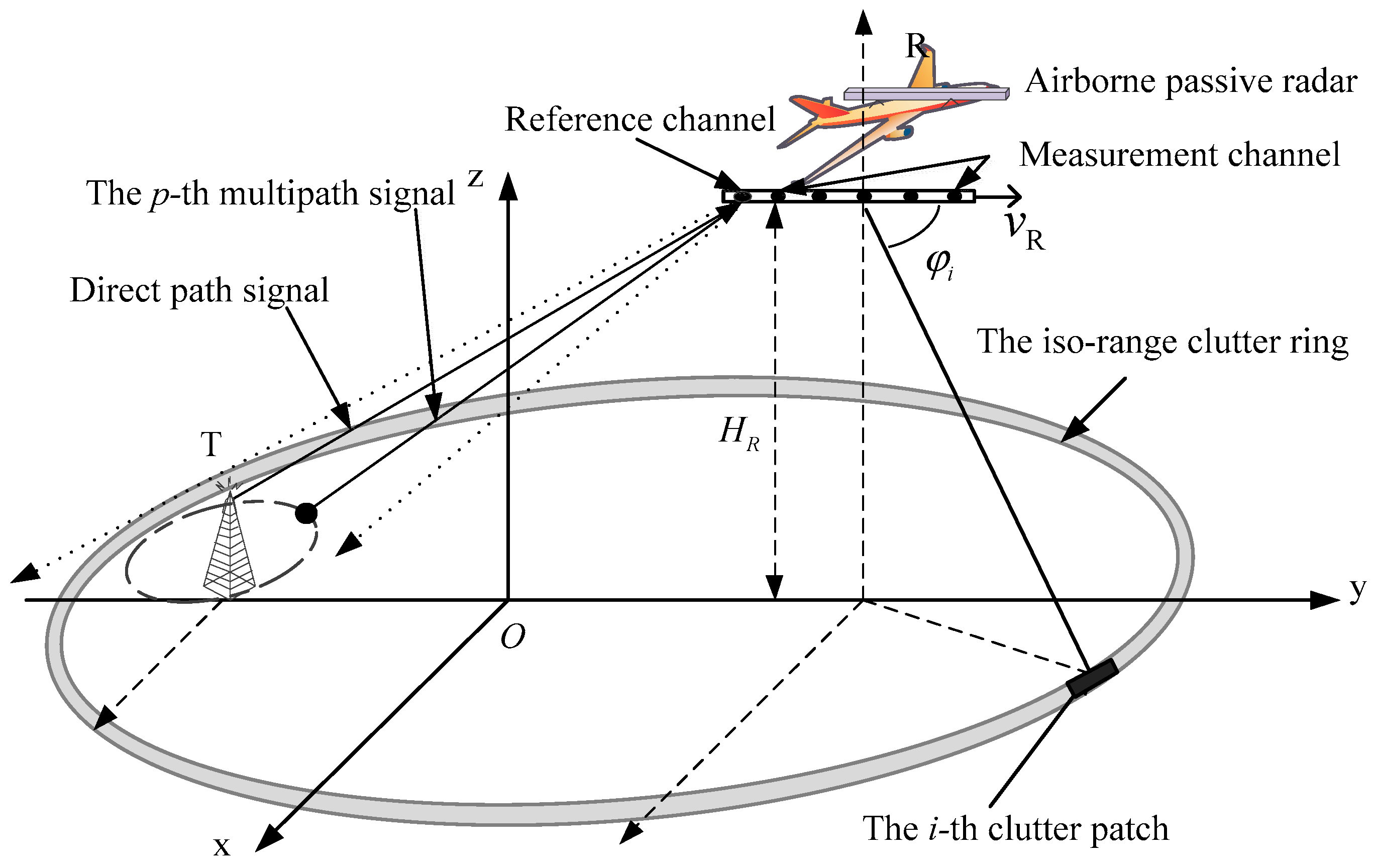
3. Signal Model
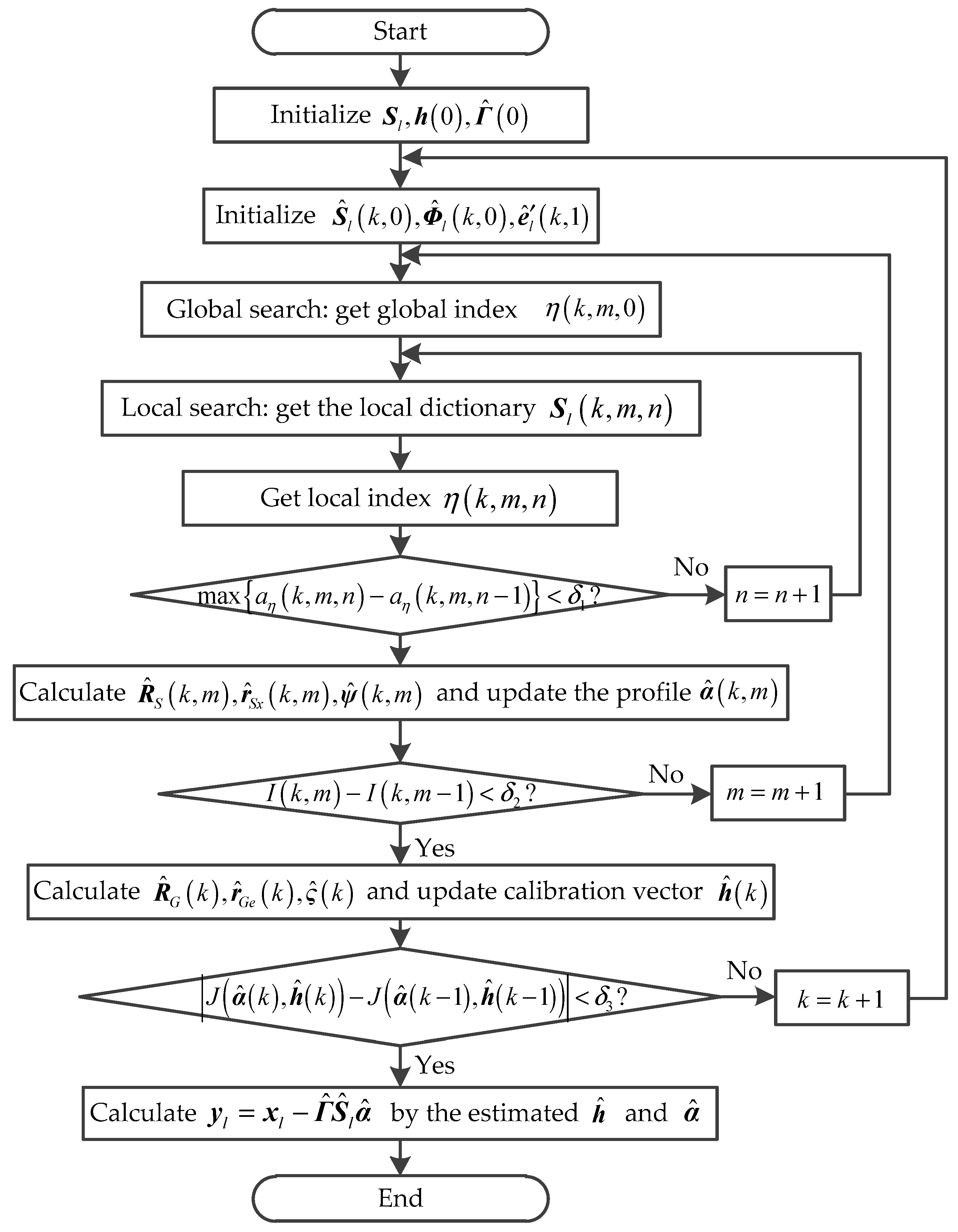
4. Proposed MP Clutter Suppression Algorithm Based on Joint Optimization
4.1. Review of the Existing Optimization Problem in SRA and LSA
4.2. The Motivation of the Proposed Joint Optimization Algorithm
4.3. The Proposed Joint Optimization Algorithm
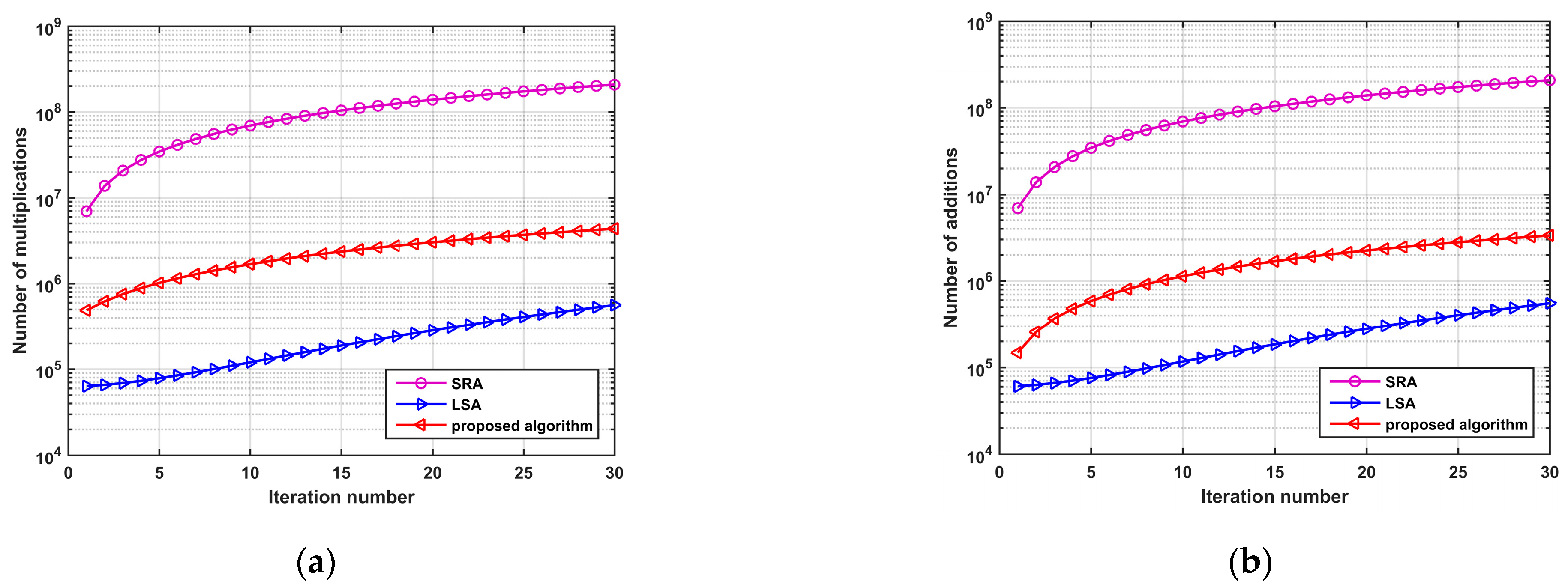
4.4. Analyses of Computational Complexity
5. Simulations and Performance Analyses
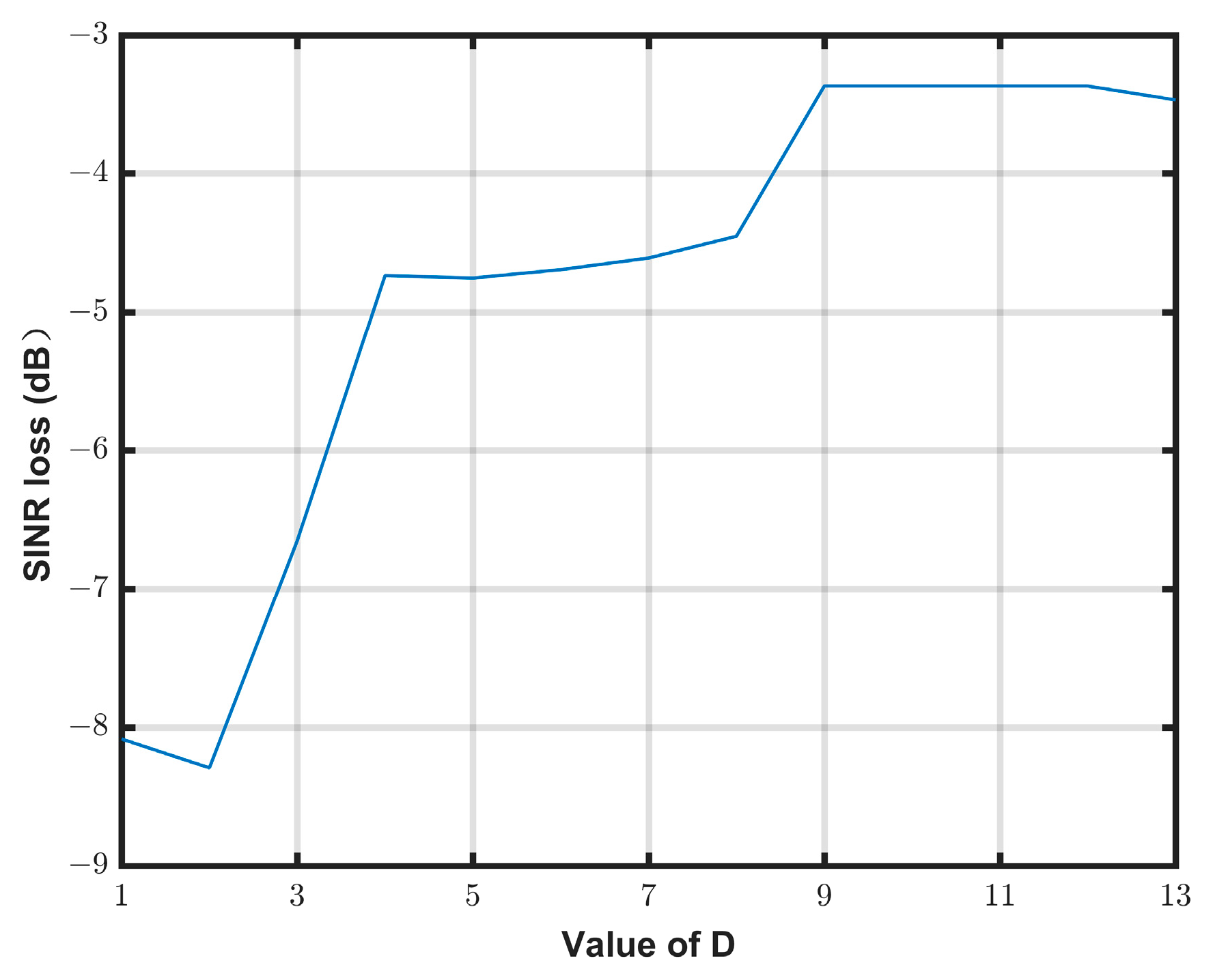
5.1. Selection of the Number of Snapshots D
5.2. Setting of the Alternation Threshold
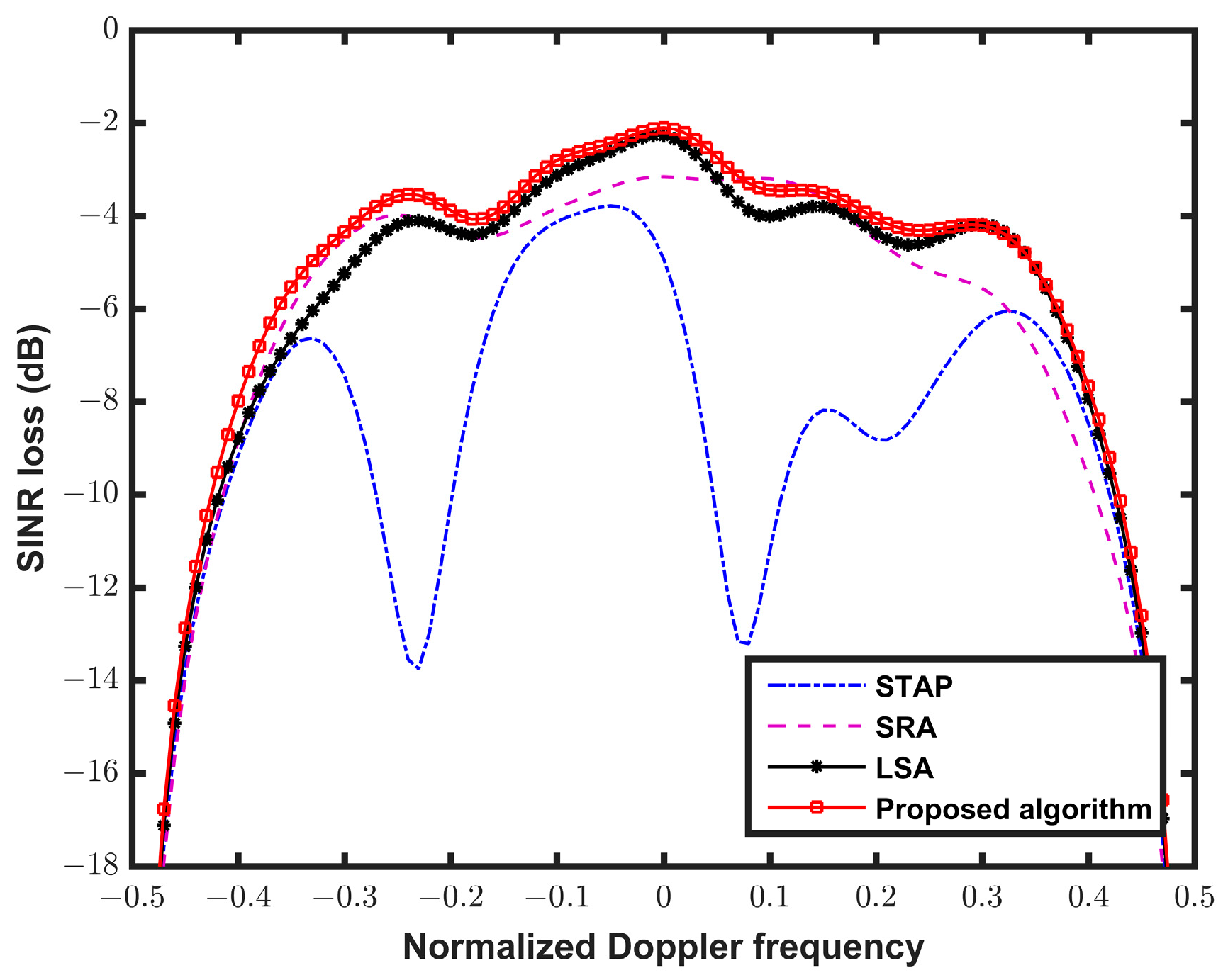
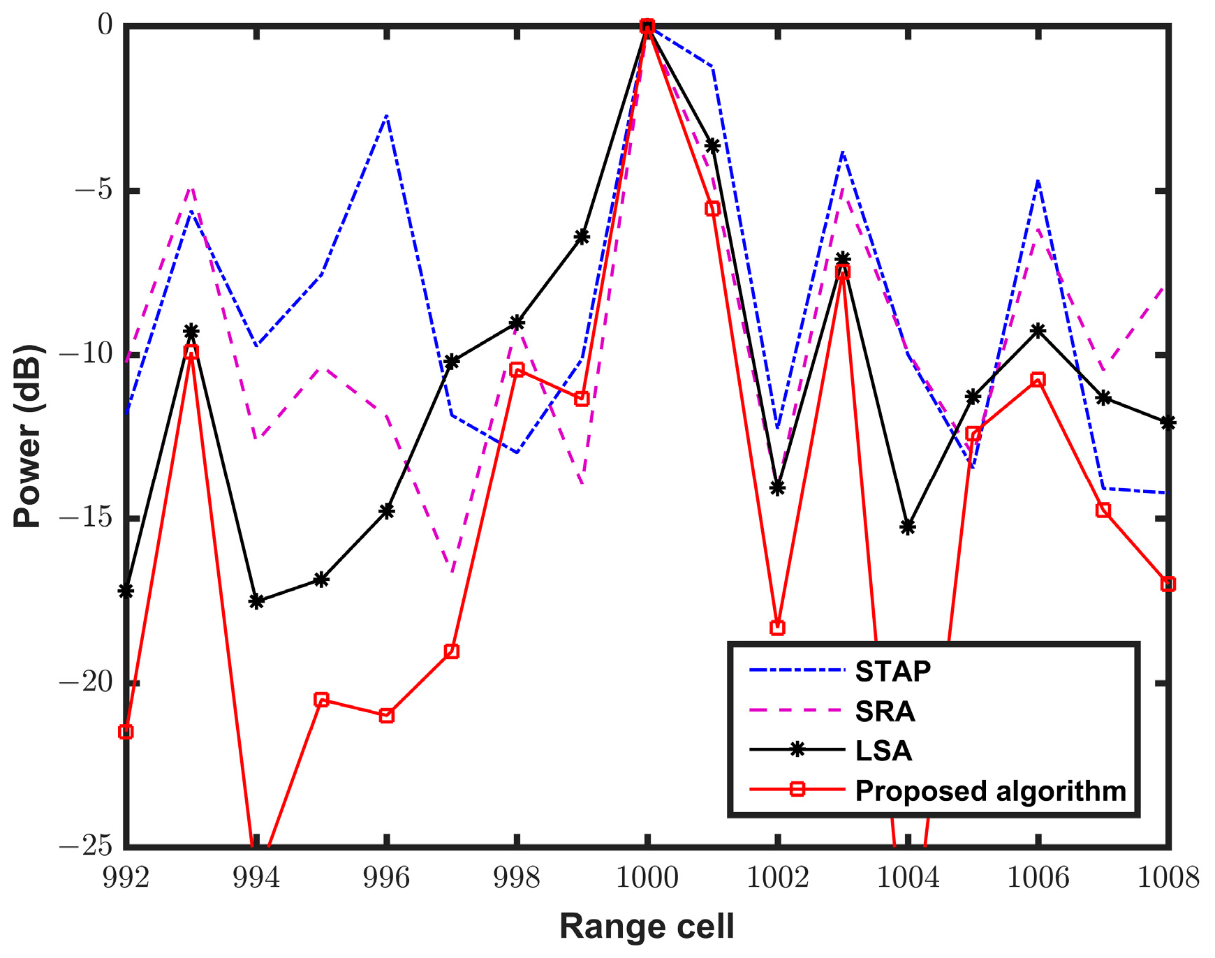
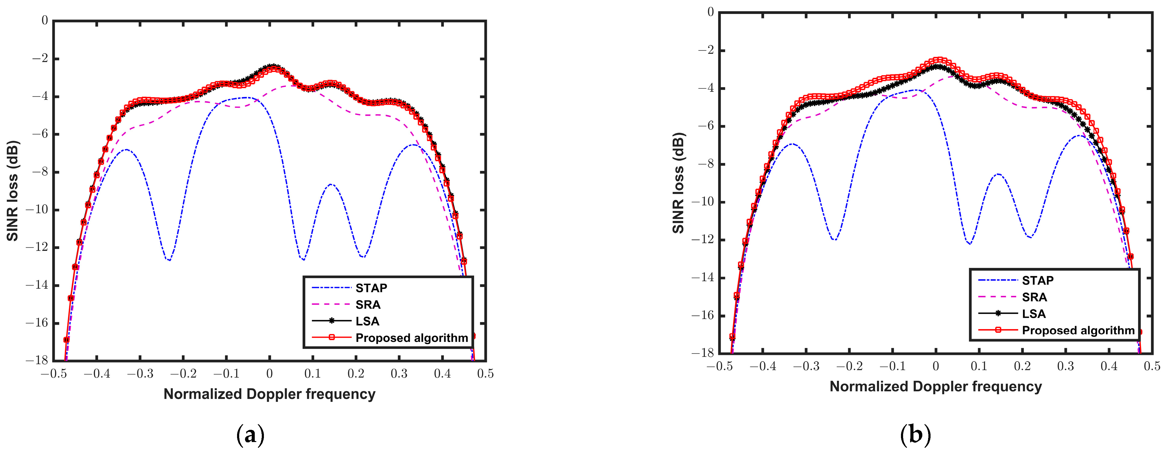
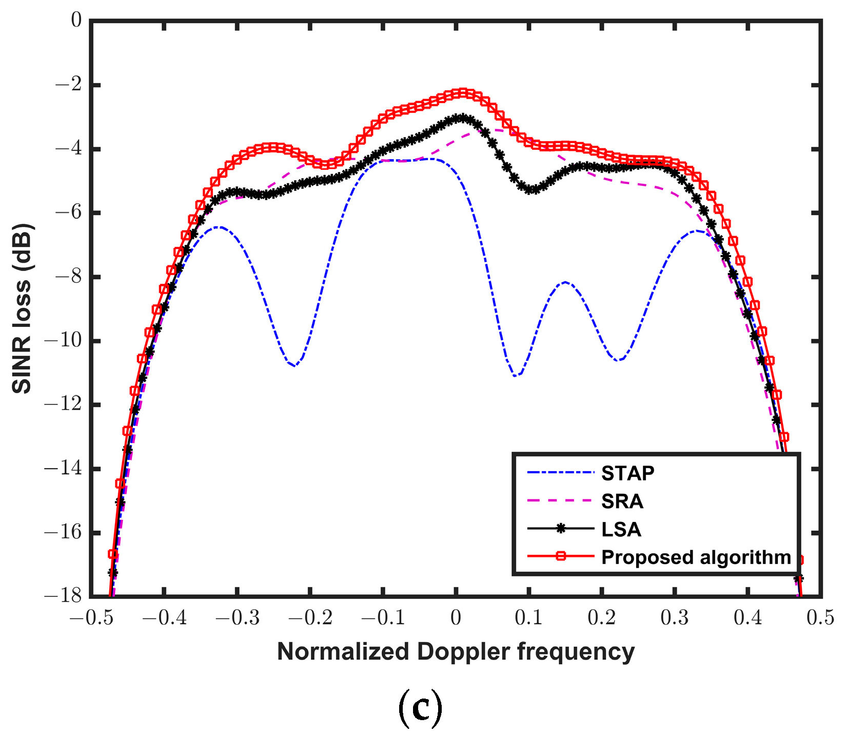
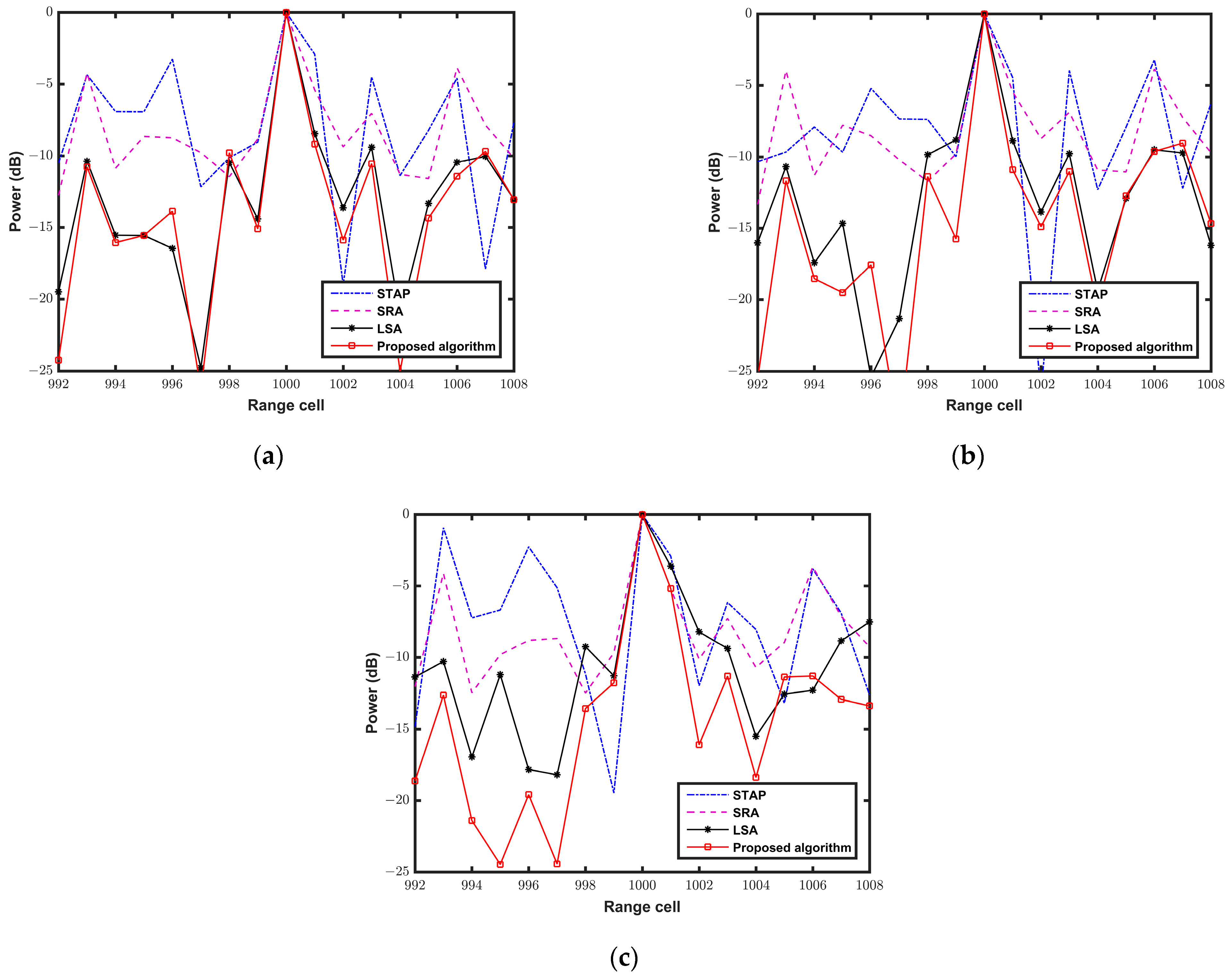
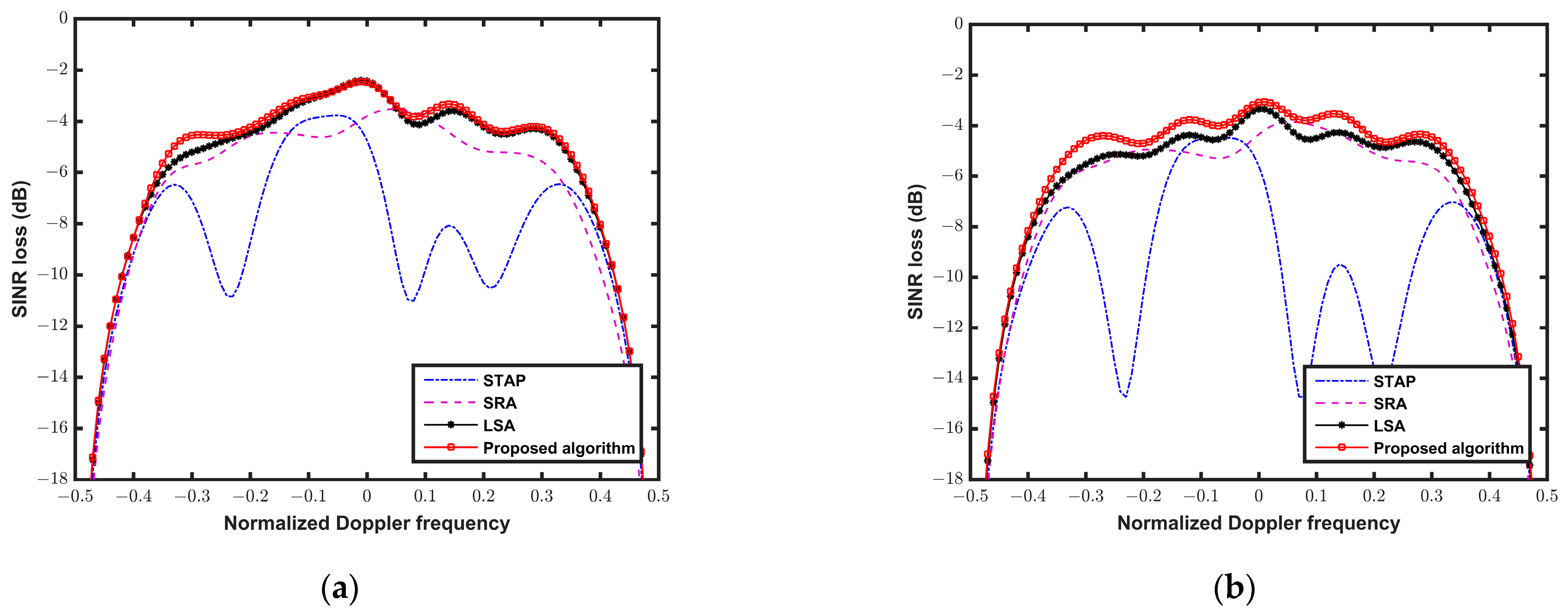
5.3. Comparison with the Exiting Methods
6. Conclusions
Author Contributions
Funding
Institutional Review Board Statement
Informed Consent Statement
Data Availability Statement
Conflicts of Interest
References
- Malanowski, M.; Rytel-Andrianik, R.; Kulpa, K.; Stasiak, K.; Ciesielski, M.; Kulpa, J. Geometric clutter analysis for airborne passive coherent location radar. IEEE Trans. Geosci. Remote Sens. 2022, 60, 5116314. [Google Scholar] [CrossRef]
- Tan, D.K.P.; Lesturgie, M.; Sun, H.; Lu, Y. Space–time interference analysis and suppression for airborne passive radar using transmissions of opportunity. IET Radar Sonar Navig. 2014, 8, 142–152. [Google Scholar] [CrossRef]
- Wojaczek, P.; Colone, F.; Cristallini, D.; Lombardo, P. Reciprocal-Filter-Based STAP for Passive Radar on Moving Platforms. IEEE Trans. Aerosp. Electron. Syst. 2019, 55, 967–988. [Google Scholar] [CrossRef]
- Rosenberg, L.; Duk, V. Land clutter statistics from an airborne passive bistatic radar. IEEE Trans. Geosci. Remote Sens. 2022, 60, 5104009. [Google Scholar] [CrossRef]
- Sui, J.; Wang, J.; Zuo, L.; Gao, J. Cascaded least square algorithm for strong clutter removal in airborne passive radar. IEEE Trans. Aerosp. Electron. Syst. 2022, 58, 679–696. [Google Scholar] [CrossRef]
- Brown, J.; Woodbridge, K.; Griffiths, H.; Stove, A.; Watts, S. Passive bistatic radar experiments from an airborne platform. IEEE Aerosp. Electron. Syst. Mag. 2012, 27, 50–55. [Google Scholar] [CrossRef]
- Sui, J.; Wang, J.; Zuo, L.; Gao, J. Multistage least squares algorithms for clutter suppression in airborne passive radar based on subband operation. IEEE Trans. Aerosp. Electron. Syst. 2023, 59, 1893–1909. [Google Scholar] [CrossRef]
- Deng, Y.; Wang, J.; Luo, Z.; Guo, S. Cascaded suppression method for airborne passive radar with contaminated reference signal. IEEE Access 2019, 7, 50317–50329. [Google Scholar] [CrossRef]
- Guo, S.; Wang, J.; Ma, H.; Wang, J. Modified blind equalization algorithm based on cyclostationarity for contaminated referent signal in airborne PBR. Sensors 2020, 20, 788. [Google Scholar] [CrossRef]
- Deng, Y.; Zhang, S.; Zhu, Q.; Zhang, L.; Li, W. Clutter suppression methods based on reduced-dimension transformation for airborne passive radar with impure reference signals. J. Appl. Remote Sens. 2021, 15, 016514. [Google Scholar] [CrossRef]
- Deng, Y.; Li, W.; Zhang, S.; Wang, F.; Xiao, W.; Cui, Z. Clutter suppression method for off-grid effects mitigation in airborne passive radars with contaminated reference signals. Sensors 2021, 21, 6339. [Google Scholar] [CrossRef]
- Ward, J. Space-Time Adaptive Processing for Airborne Radar. In Proceedings of the IEE Colloquium on Space-Time Adaptive Processing, London, UK, 6 April 1998. [Google Scholar]
- Klemm, R. Principles of Space-Time Adaptive Processing, 3rd ed.; Institute of Electical Engineering: London, UK, 2006. [Google Scholar]
- Mevin, W.L.; Showman, G.A. An approach to knowledge-aided covariance estimation. IEEE Trans. Aerosp. Electron. Syst. 2006, 42, 1021–1042. [Google Scholar] [CrossRef]
- Liu, M.; Zou, L.; Yu, X.; Zhou, Y.; Wang, X.; Tang, B. Knowledge aided covariance matrix estimation via gaussian Kernel function for airborne SR-STAP. IEEE Access 2020, 8, 5970–5978. [Google Scholar] [CrossRef]
- Riedl, M.; Potter, L.C. Multimodel shrinkage for knowledge-aided space-time adaptive processing. IEEE Trans. Aerosp. Electron. Syst. 2018, 54, 2601–2610. [Google Scholar] [CrossRef]
- Hu, J.; Li, J.; Li, H.; Li, K.; Liang, J. A novel covariance matrix estimation via cyclic characteristic for STAP. IEEE Geosci. Remote Sens. Lett. 2020, 17, 1871–1875. [Google Scholar] [CrossRef]
- Liu, C.; Wang, T.; Zhang, S.; Ren, B. A clutter suppression algorithm via weighted l2−norm penalty for airborne radar. IEEE Signal Process. Lett. 2022, 29, 1522–1525. [Google Scholar] [CrossRef]
- Zhou, Y.; Wang, L.; Chen, X.; Wen, C.; Jiang, B.; Fang, D. An improving EFA for clutter suppression by using the persymmetric covariance matrix estimation. Circuits Syst. Signal Process. 2018, 37, 4136–4149. [Google Scholar] [CrossRef]
- Cui, N.; Duan, K.; Xing, K.; Yu, Z. Beam-space reduced-dimension 3D-STAP for nonside-looking airborne radar. IEEE Geosci. Remote Sens. Lett. 2022, 19, 3506505. [Google Scholar] [CrossRef]
- Shen, S.; Tang, L.; Nie, X.; Bai, Y.; Zhang, X.; Li, P. Robust space time adaptive processing methods for synthetic aperture radar. Appl. Sci. 2020, 10, 3609. [Google Scholar] [CrossRef]
- Shen, M.; Zhu, D.; Zhu, Z. Reduced-rank space-time adaptive processing using a modified projection approximation subspace tracking deflation approach. IET Radar Sonar Navig. 2009, 3, 93–100. [Google Scholar] [CrossRef]
- Huang, P.; Zou, Z.; Xia, X.; Liu, X.; Liao, G. A novel dimension-reduced space–time adaptive processing algorithm for spaceborne multichannel surveillance radar systems based on spatial–temporal 2-D sliding window. IEEE Trans. Geosci. Remote Sens. 2022, 60, 5109721. [Google Scholar] [CrossRef]
- Shi, J.; Xie, L.; Cheng, Z.; He, Z.; Zhang, W. Angle-Doppler channel selection method for reduced-dimension STAP based on sequential convex programming. IEEE Comm. Lett. 2021, 25, 3080–3084. [Google Scholar] [CrossRef]
- Chen, W.; Xie, W.; Wang, Y. Short-range clutter suppression for airborne radar using sparse recovery and orthogonal projection. IEEE Geosci. Remote Sens. Lett. 2022, 19, 3500605. [Google Scholar] [CrossRef]
- Xie, L.; He, Z.; Tong, J.; Zhang, W. A recursive angle-Doppler channel selection method for reduced-dimension space-time adaptive processing. IEEE Trans. Aerosp. Electron. Syst. 2020, 56, 3985–4000. [Google Scholar] [CrossRef]
- Yang, Z.; de Lamare, R.C.; Li, X. L1-regularized STAP algorithms with a generalized sidelobe canceler architecture for airborne radar. IEEE Trans. Signal Process. 2012, 60, 674–686. [Google Scholar] [CrossRef]
- Wang, X.; Yang, Z.; Huang, J.; de Lamare, R.C. Robust two-stage reduced-dimension sparsity-aware STAP for airborne radar with coprime arrays. IEEE Trans. Signal Process. 2020, 68, 81–96. [Google Scholar] [CrossRef]
- Li, X.; Yang, X.; Wang, Y.; Duan, K. Gridless sparse clutter nulling STAP based on particle swarm optimization. IEEE Geosci. Remote Sens. Lett. 2022, 19, 4023205. [Google Scholar] [CrossRef]
- Zhang, W.; An, R.; He, N.; He, Z.; Li, H. Reduced dimension STAP based on sparse recovery in heterogeneous clutter environments. IEEE Trans. Aerosp. Electron. Syst. 2020, 56, 785–795. [Google Scholar] [CrossRef]
- Hu, Z.; Wang, W.; Dong, F. A low-complexity MIMO radar STAP strategy for efficient sea clutter suppression. IEEE Geosci. Remote Sens. Lett. 2022, 19, 4024105. [Google Scholar] [CrossRef]
- Cui, N.; Xing, K.; Yu, Z.; Duan, K. Tensor-based sparse recovery space-time adaptive processing for large size data clutter suppression in airborne radar. IEEE Trans. Aerosp. Electron. Syst. 2023, 59, 907–922. [Google Scholar] [CrossRef]
- Duan, K.; Chen, H.; Xie, W.; Wang, Y. Deep learning for high-resolution estimation of clutter angle-Doppler spectrum in STAP. IET Radar Sonar Navig. 2022, 16, 193–207. [Google Scholar] [CrossRef]
- Zou, B.; Wang, X.; Feng, W.; Zhu, H.; Lu, F. DU-CG-STAP method based on sparse recovery and unsupervised learning for airborne radar clutter suppression. Remote Sens. 2022, 14, 3472. [Google Scholar] [CrossRef]
- Yang, Z.; Qin, Y.; de Lamare, R.C.; Wang, H.; Li, X. Sparsity-based direct data domain space-time adaptive processing with intrinsic clutter motion. Circuits Syst. Signal Process. 2017, 36, 219–246. [Google Scholar] [CrossRef]
- Yang, Z.; Li, X.; Wang, H.; Fa, R. Knowledge-aided STAP with sparse-recovery by exploiting spatio-temporal sparsity. IET Signal Process. 2016, 10, 150–161. [Google Scholar] [CrossRef]
- Gu, Y.; Wu, J.; Fang, Y.; Zhang, L.; Zhang, Q. End-to-end moving target indication for airborne radar using deep learning. Remote Sens. 2022, 14, 5354. [Google Scholar] [CrossRef]
- Duan, K.; Liu, W.; Duan, G.; Wang, Y. Off-grid effects mitigation exploiting knowledge of the clutter ridge for sparse recovery STAP. IET Radar Sonar Navig. 2018, 12, 557–564. [Google Scholar] [CrossRef]
- Ma, Z.; Liu, Y.; Meng, H.; Wang, X. Sparse recovery-based space-time adaptive processing with array error self-calibration. Electron. Lett. 2014, 50, 952–954. [Google Scholar] [CrossRef]
- Yang, Z.; de Lamare, R.C.; Liu, W. Sparsity-based STAP using alternating direction method with gain/phase errors. IEEE Trans. Aerosp. Electron. Syst. 2017, 53, 2756–2768. [Google Scholar]


| Parameter | Value |
|---|---|
| Number of spatial elements | 10 |
| Number of temporal pulses | 10 |
| Antenna array | Side-looking array |
| inter-channel spacing | |
| Pulse repetition interval | 2.5 ms |
| Platform velocity | 100 m/s |
| Number of clutter patches in each range cell | 181 |
| Range cell index of target | 1000 |
| Normalized Doppler frequency of target | −0.28 |
| Signal-to-noise ratio of target | 0 dB |
| Index | True 1 | True 2 | True 3 | Ghost 1 | Ghost 2 | Ghost 3 |
|---|---|---|---|---|---|---|
| Real atoms | [3, 0.23] | [4, −0.08] | [9, −0.22] | [6, 0.46] | [7, 0.15] | [8, −0.16] |
| LSA | [3, 0.234] | [4, −0.0795] | [9, −0.2164] | [6, 0.4738] | [7, 0.1773] | [1, 0.05] |
| Proposed method | [3, 0.2328] | [4, −0.0805] | [9, −0.218] | [6, 0.4727] | [7, 0.1758] | [8, −0.1797] |
| 0.2 | 0.6 | 1.0 | 1.4 | 1.8 | |
|---|---|---|---|---|---|
| SRA (dB) | −5.046 | −5.032 | −5.097 | −5.104 | −5.096 |
| LSA (dB) | −4.451 | −4.827 | −5.115 | −5.481 | −5.668 |
| Proposed algorithm (dB) | −4.278 | −4.321 | −4.318 | −4.432 | −4.417 |
| MDR Value (dB) | −15 | −19 | −23 | −27 | −31 |
|---|---|---|---|---|---|
| SRA (dB) | −5.321 | −5.032 | −4.957 | −4.915 | −4.876 |
| LSA (dB) | −5.228 | −4.867 | −4.565 | −4.348 | −4.084 |
| Proposed algorithm (dB) | −4.656 | −4.444 | −4.268 | −4.032 | −4.081 |
Disclaimer/Publisher’s Note: The statements, opinions and data contained in all publications are solely those of the individual author(s) and contributor(s) and not of MDPI and/or the editor(s). MDPI and/or the editor(s) disclaim responsibility for any injury to people or property resulting from any ideas, methods, instructions or products referred to in the content. |
© 2023 by the authors. Licensee MDPI, Basel, Switzerland. This article is an open access article distributed under the terms and conditions of the Creative Commons Attribution (CC BY) license (https://creativecommons.org/licenses/by/4.0/).
Share and Cite
Deng, Y.; Pei, Z.; Li, W.; Jiang, D. Clutter Suppression Algorithm with Joint Intrinsic Clutter Motion Errors Calibration and Off-Grid Effects Mitigation in Airborne Passive Radars. Appl. Sci. 2023, 13, 5653. https://doi.org/10.3390/app13095653
Deng Y, Pei Z, Li W, Jiang D. Clutter Suppression Algorithm with Joint Intrinsic Clutter Motion Errors Calibration and Off-Grid Effects Mitigation in Airborne Passive Radars. Applied Sciences. 2023; 13(9):5653. https://doi.org/10.3390/app13095653
Chicago/Turabian StyleDeng, Yaqi, Zhengwang Pei, Wenguo Li, and Dongchu Jiang. 2023. "Clutter Suppression Algorithm with Joint Intrinsic Clutter Motion Errors Calibration and Off-Grid Effects Mitigation in Airborne Passive Radars" Applied Sciences 13, no. 9: 5653. https://doi.org/10.3390/app13095653