
GEOBIA and Vegetation Indices in Extracting Olive Tree Canopies Based on Very High-Resolution UAV Multispectral Imagery

 ,
,  ,
,  ,
,  ,
,  ,
,  ,
,  and
and 
Abstract
:
1. Introduction
2. Materials and Methods
2.1. Study Area
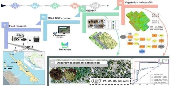
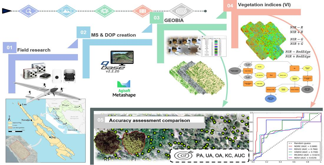
2.2. The Methodological Framework
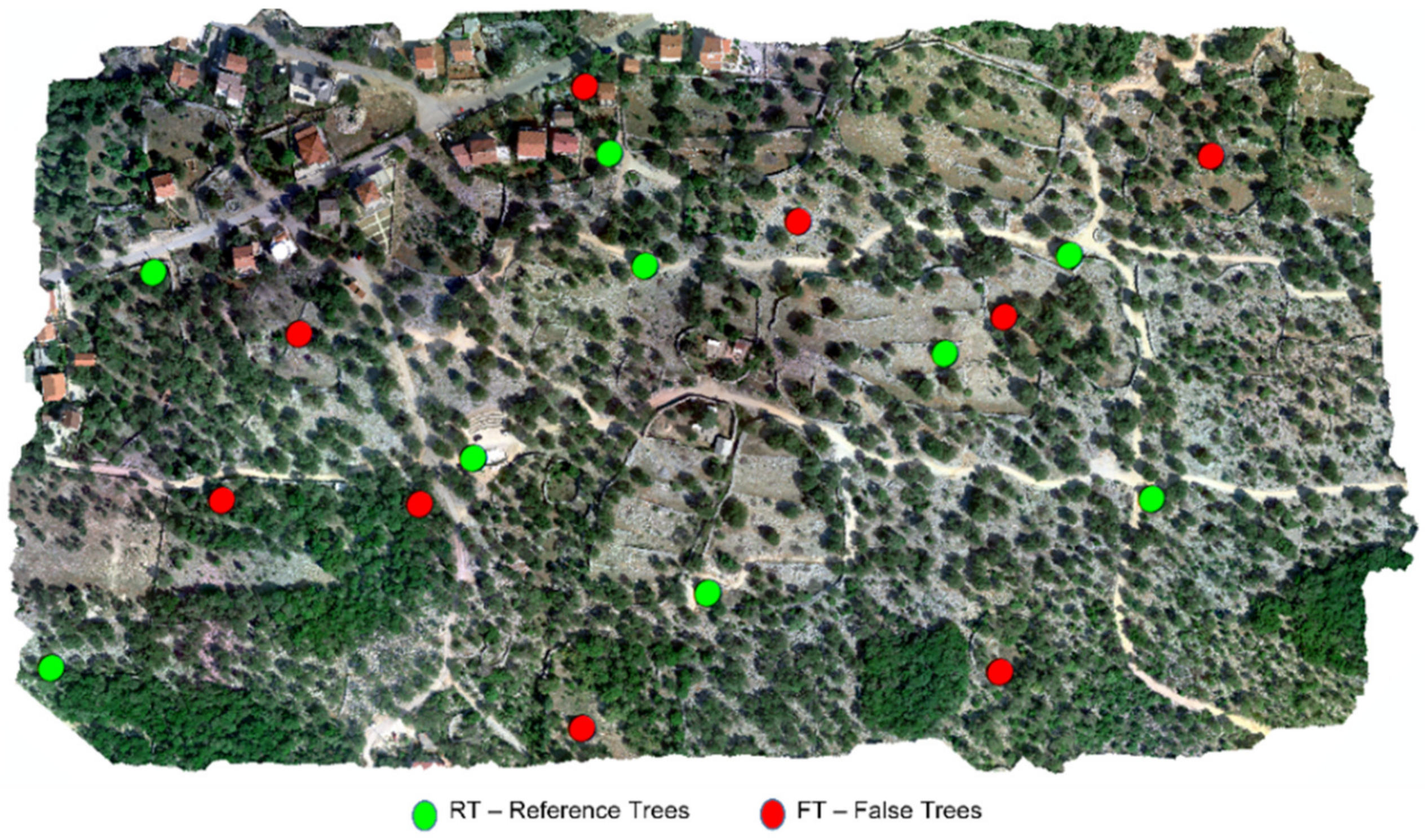
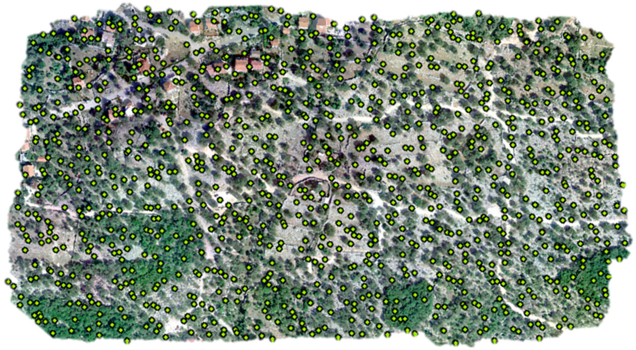
2.3. Field Research
2.4. Data Acquisition
2.5. UAV Imagery Processing
2.6. GEOBIA
2.6.1. MS Bands Layout
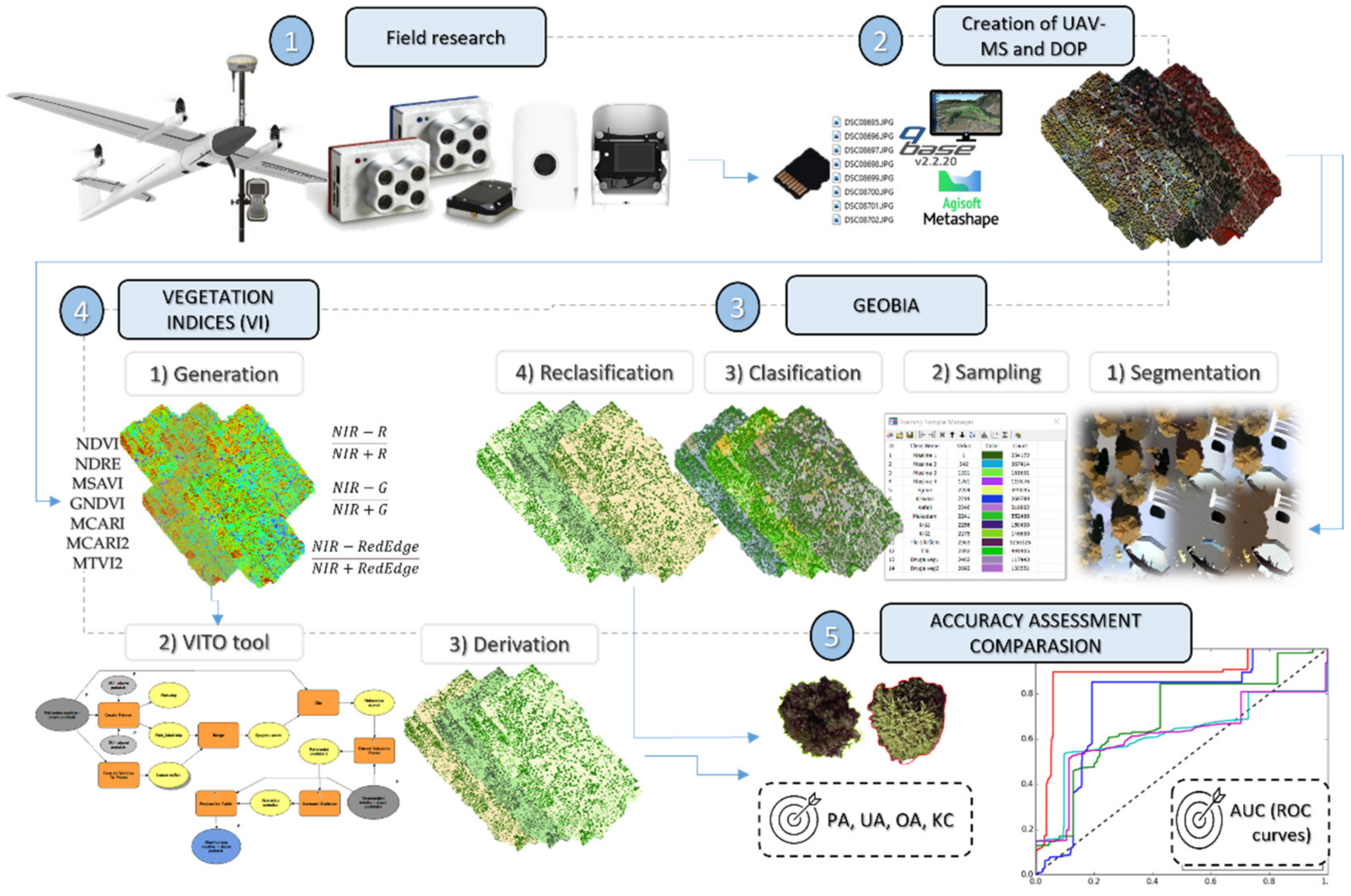
2.6.2. Segmentation
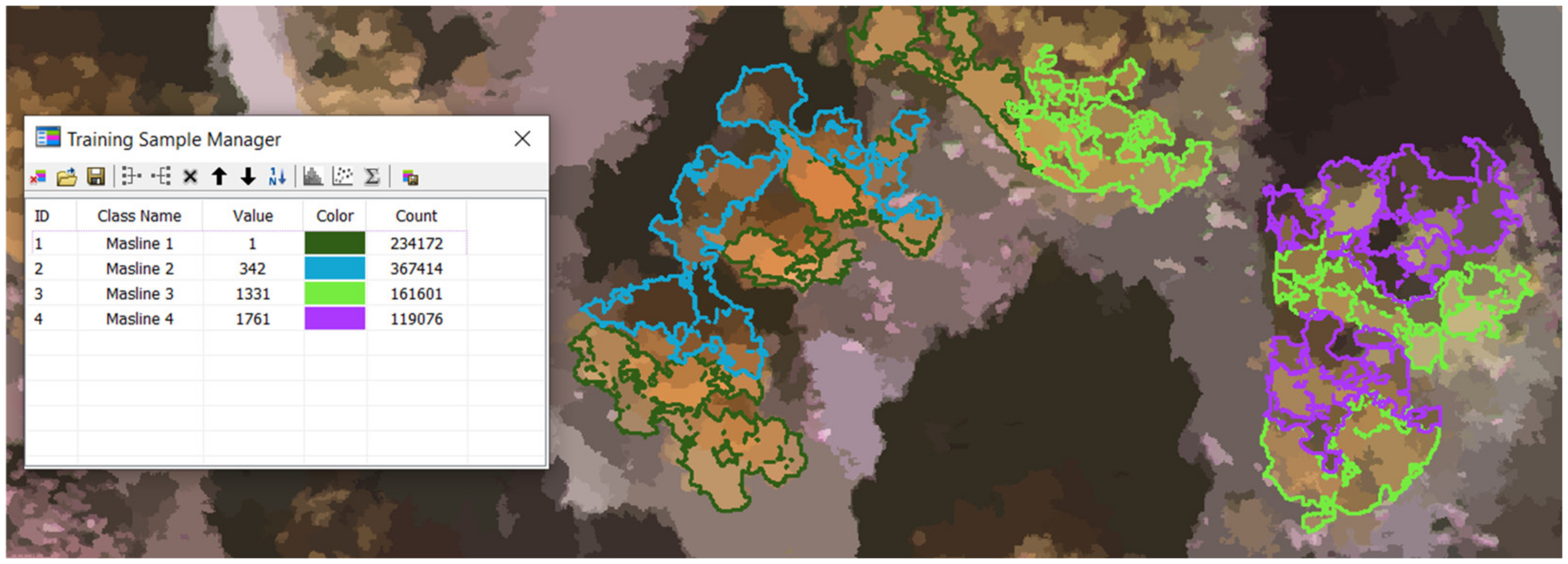
2.6.3. Test Samples
2.6.4. Classification
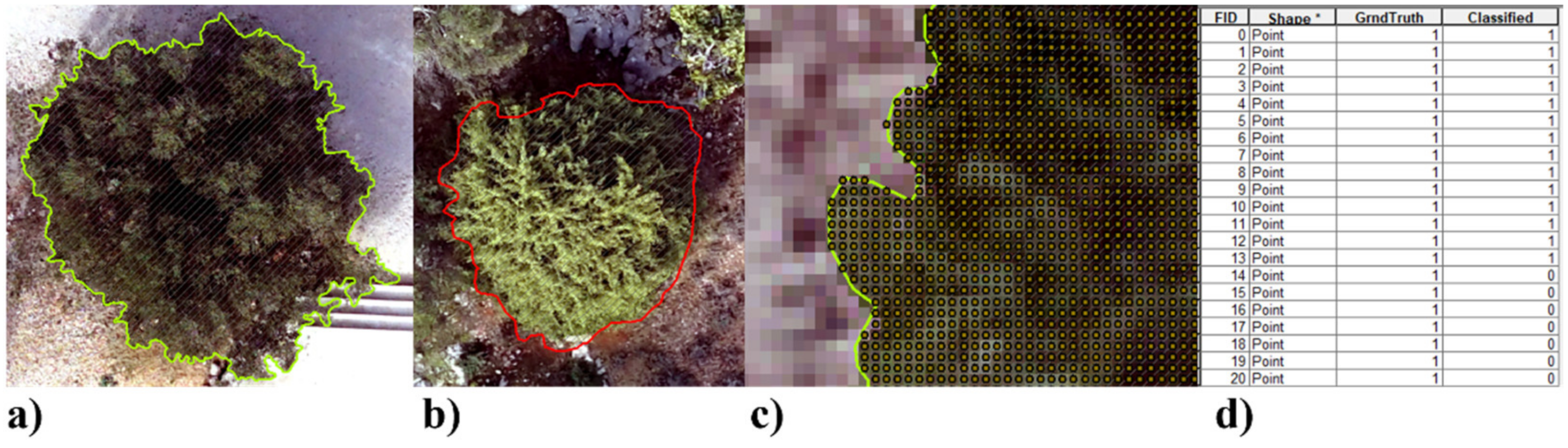
2.6.5. Accuracy Assessment
2.7. Vegetation Indices (VI)
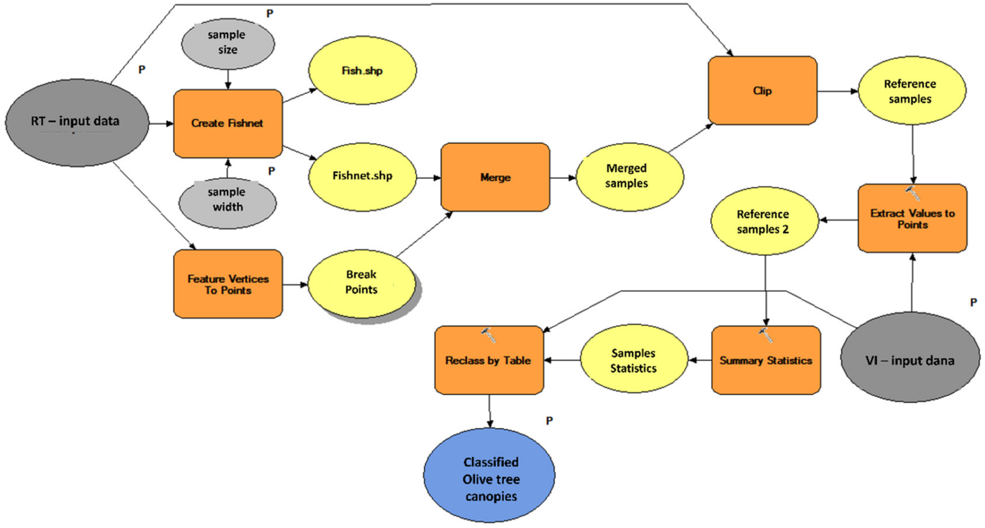
2.7.1. VITO Tool
2.7.2. Accuracy Assessment
2.8. Comparison of Classification Approaches
3. Results and Discussion
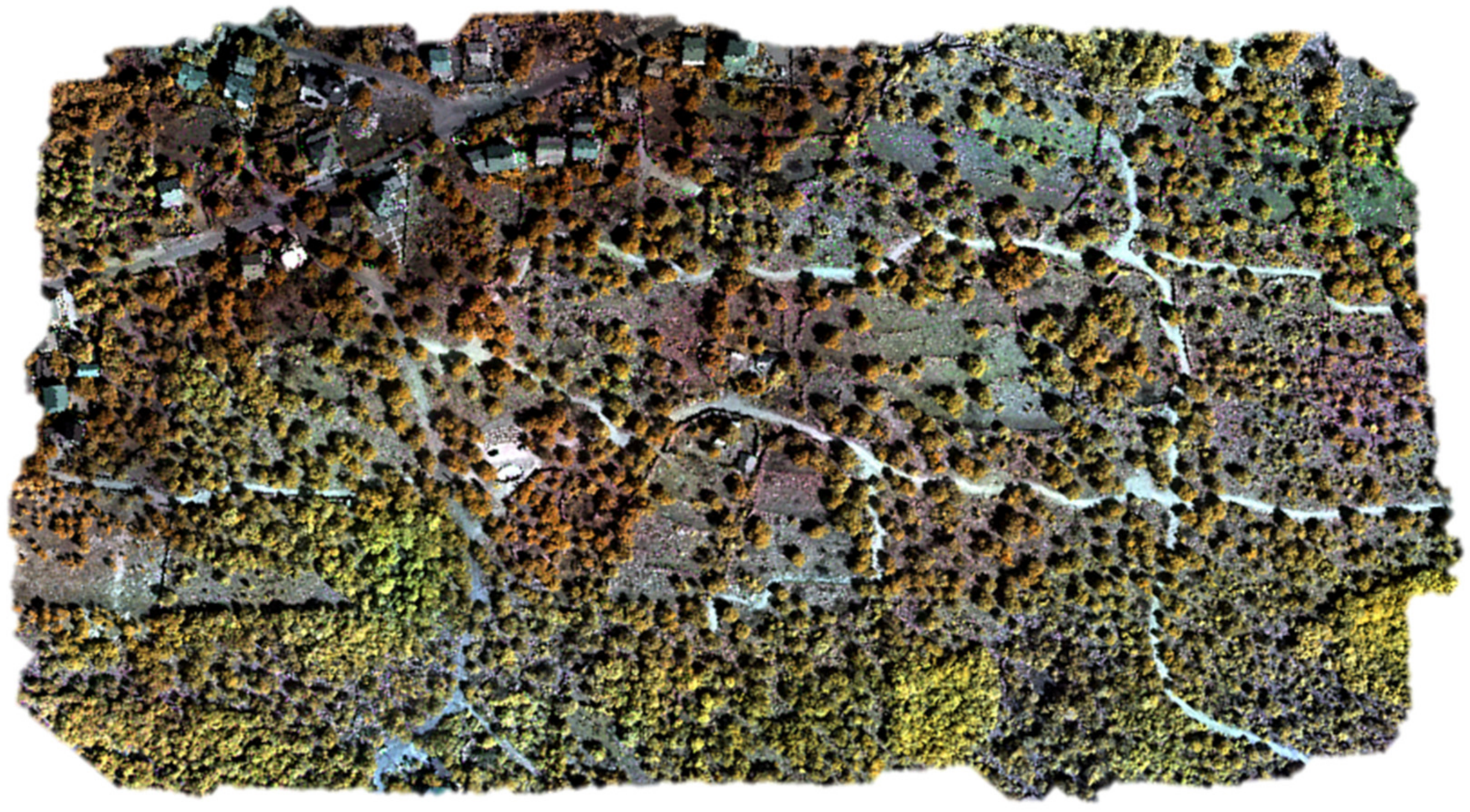
3.1. UAV-MS and DOP Creation
3.2. GEOBIA
3.2.1. Segmentation
3.2.2. Test Samples
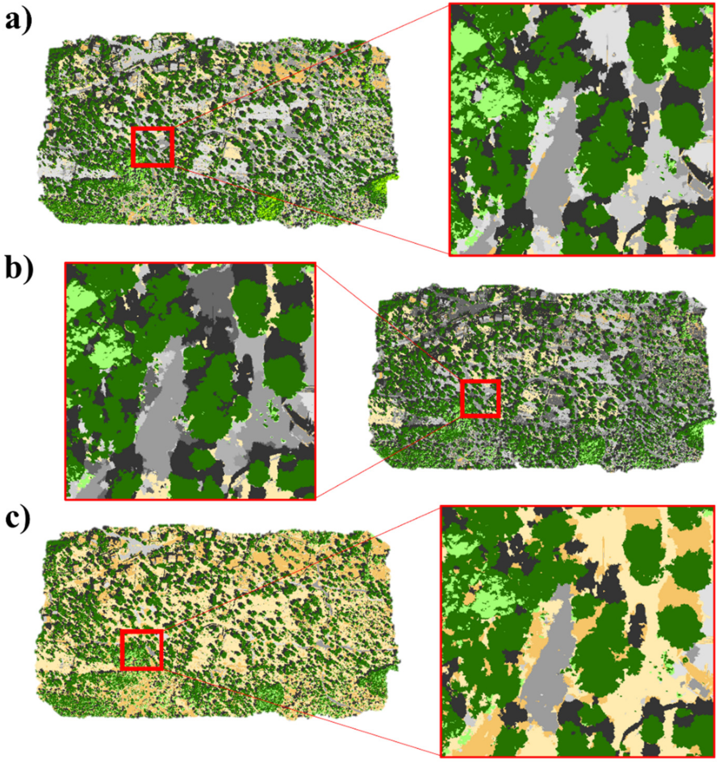
3.2.3. Results of Classification Algorithms
3.2.4. Accuracy of Classification Algorithms
3.3. Vegetation Indices
3.3.1. Derived VIs Models
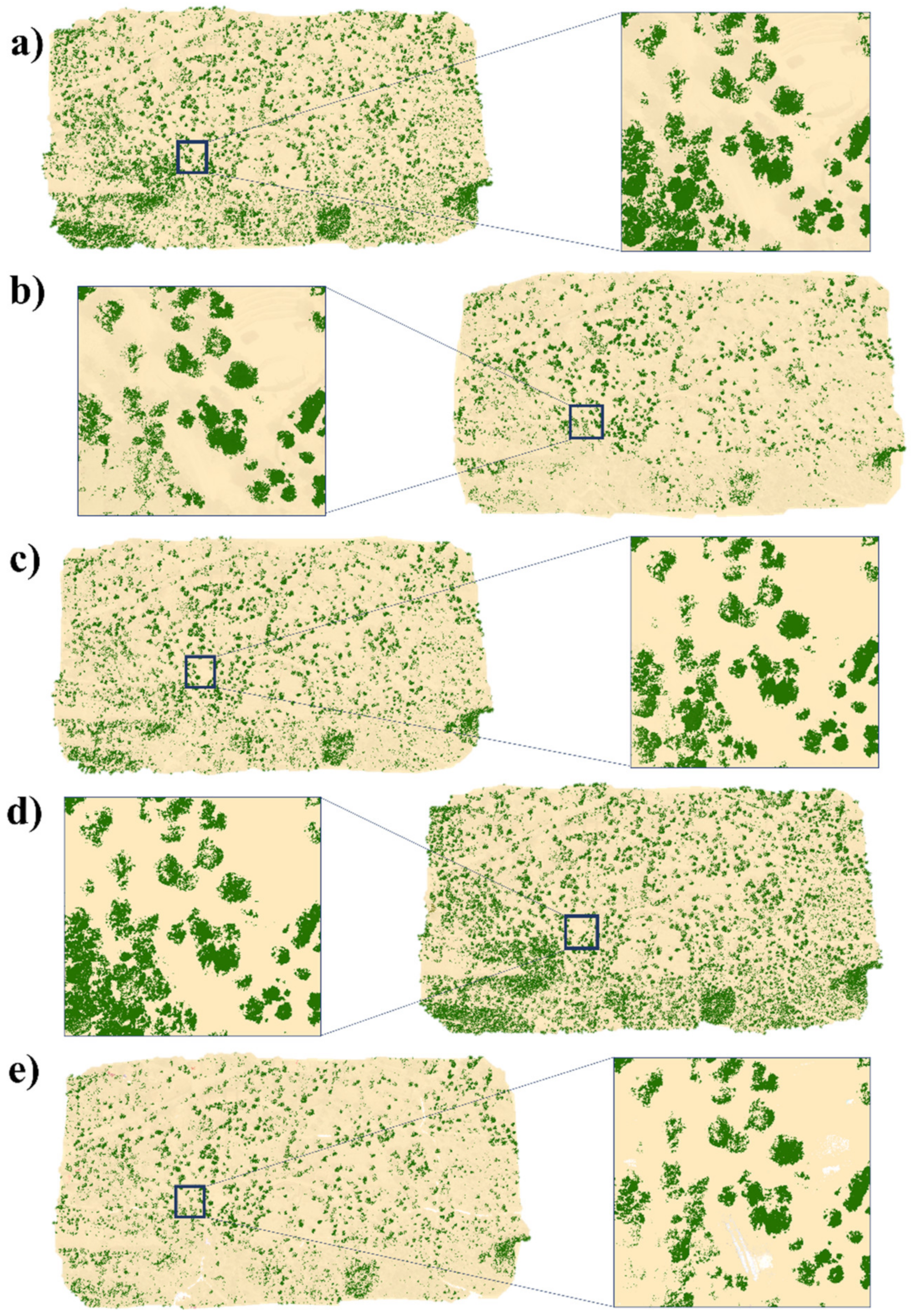
3.3.2. VITO Tool Results
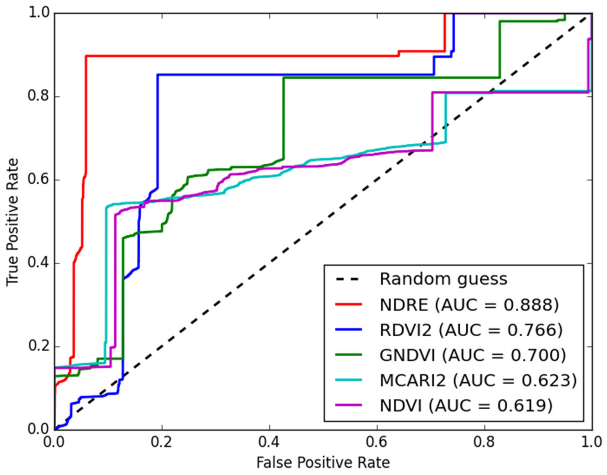
3.3.3. Accuracy of VIs Models
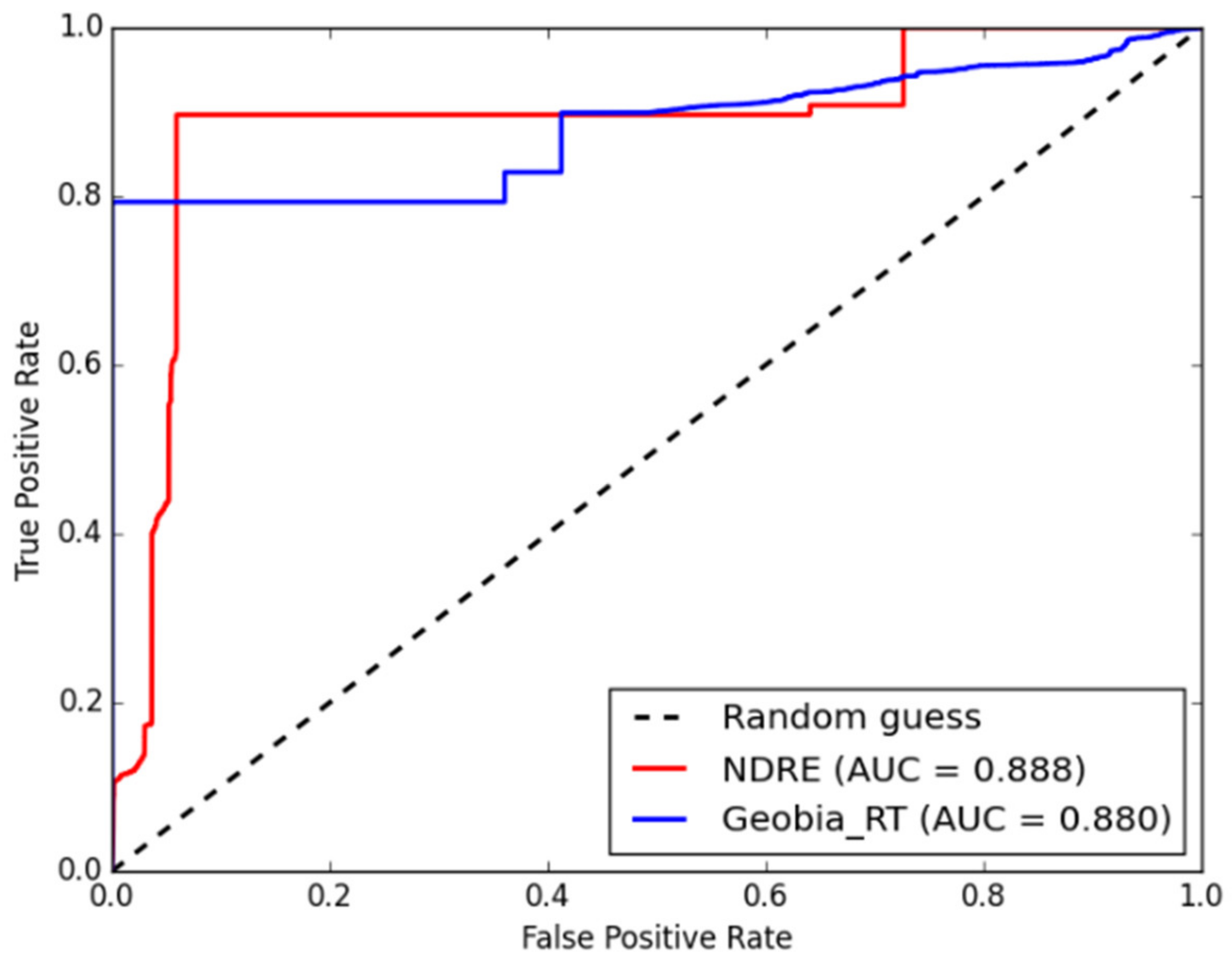
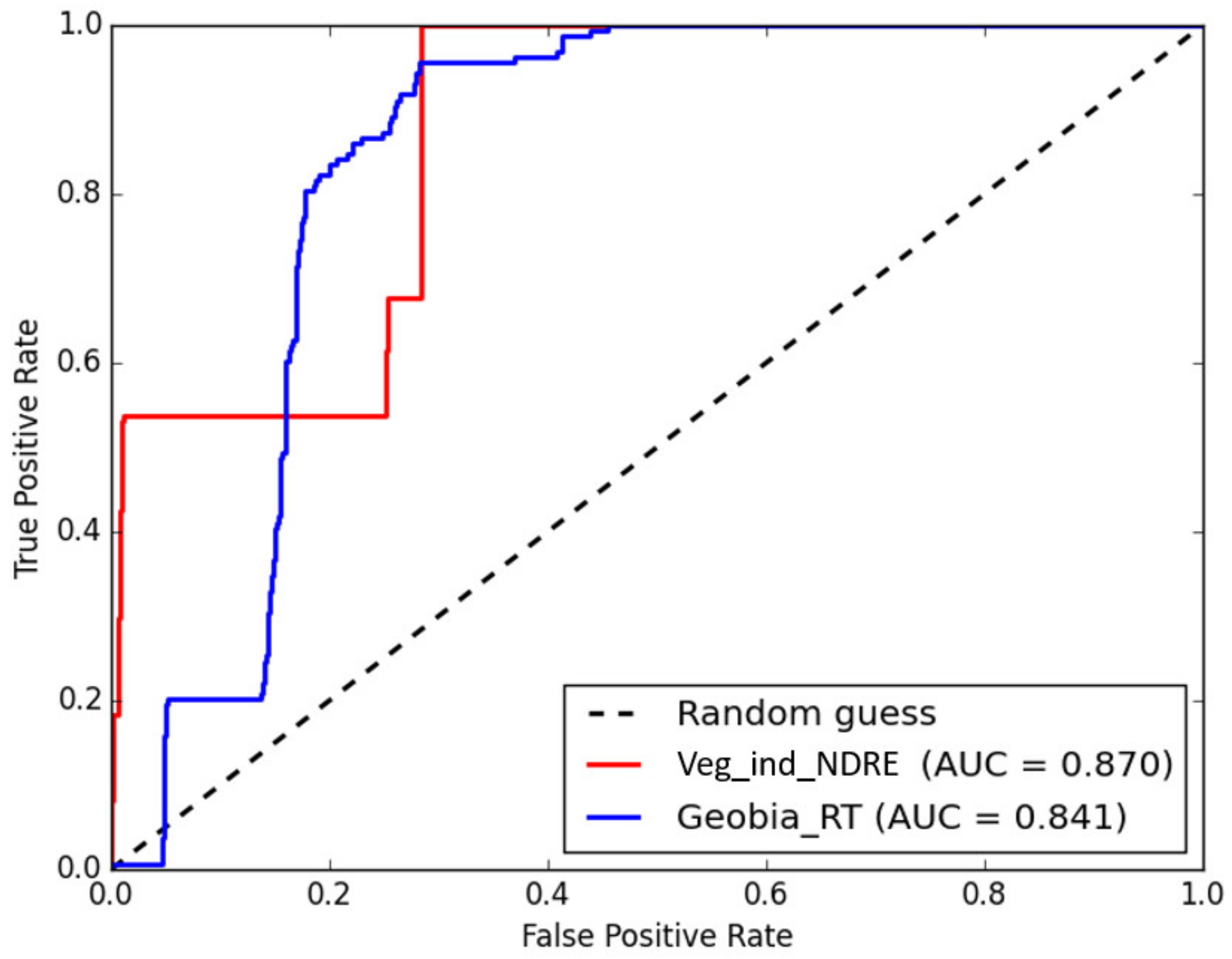
3.4. Results of Used Approaches Comparison
4. Conclusions
Author Contributions
Funding
Institutional Review Board Statement
Informed Consent Statement
Data Availability Statement
Acknowledgments
Conflicts of Interest
References
- Besnard, G.; Hernández, P.; Khadari, B.; Dorado, G.; Savolainen, V. Genomic Profiling of Plastid DNA Variation in the Mediterranean Olive Tree. BMC Plant Biol. 2011, 11, 80. [Google Scholar] [CrossRef] [PubMed] [Green Version]
- Díez, C.M.; Trujillo, I.; Barrio, E.; Belaj, A.; Barranco, D.; Rallo, L. Centennial Olive Trees as a Reservoir of Genetic Diversity. Ann. Bot. 2011, 108, 797–807. [Google Scholar] [CrossRef] [PubMed] [Green Version]
- Kostelenos, G.; Kiritsakis, A. Olive Tree History and Evolution. In Olives and Olive Oil as Functional Foods; John Wiley & Sons, Ltd.: St. John’s, NL, Canada, 2017; pp. 1–12. ISBN 978-1-119-13534-0. [Google Scholar]
- Potts, S.G.; Petanidou, T.; Roberts, S.; O’Toole, C.; Hulbert, A.; Willmer, P. Plant-Pollinator Biodiversity and Pollination Services in a Complex Mediterranean Landscape. Biol. Conserv. 2006, 129, 519–529. [Google Scholar] [CrossRef]
- Serra, P.; Pons, X.; Saurí, D. Land-Cover and Land-Use Change in a Mediterranean Landscape: A Spatial Analysis of Driving Forces Integrating Biophysical and Human Factors. Appl. Geogr. 2008, 28, 189–209. [Google Scholar] [CrossRef]
- Rodríguez Sousa, A.A.; Barandica, J.M.; Aguilera, P.A.; Rescia, A.J. Examining Potential Environmental Consequences of Climate Change and Other Driving Forces on the Sustainability of Spanish Olive Groves under a Socio-Ecological Approach. Agriculture 2020, 10, 509. [Google Scholar] [CrossRef]
- Fraga, H.; Moriondo, M.; Leolini, L.; Santos, J.A. Mediterranean Olive Orchards under Climate Change: A Review of Future Impacts and Adaptation Strategies. Agronomy 2020, 11, 56. [Google Scholar] [CrossRef]
- Loumou, A.; Giourga, C. Olive Groves: “The Life and Identity of the Mediterranean”. Agric. Hum. Values 2003, 20, 87–95. [Google Scholar] [CrossRef]
- Belleti, E.; Bevilaqua, V.R.; Brito, A.M.; Modesto, D.A.; Lanfredi, A.J.; Viviani, V.R.; Nantes-Cardoso, I.L. Synthesis of Bioluminescent Gold Nanoparticle–Luciferase Hybrid Systems for Technological Applications. Photochem. Photobiol. Sci. 2021, 20, 1439–1453. [Google Scholar] [CrossRef] [PubMed]
- Čurović, Ž.; Čurović, M.; Spalević, V.; Janic, M.; Sestras, P.; Popović, S.G. Identification and Evaluation of Landscape as a Precondition for Planning Revitalization and Development of Mediterranean Rural Settlements—Case Study: Mrkovi Village, Bay of Kotor, Montenegro. Sustainability 2019, 11, 2039. [Google Scholar] [CrossRef] [Green Version]
- Hernández-Mogollón, J.M.; Di-Clemente, E.; Campón-Cerro, A.M.; Folgado-Fernández, J.A. Olive Oil Tourism in the Euro-Mediterranean Area. Int. J. Euro-Mediterr. Stud. 2021, 14, 85–101. [Google Scholar]
- Calera, A.; Campos, I.; Osann, A.; D’Urso, G.; Menenti, M. Remote Sensing for Crop Water Management: From ET Modelling to Services for the End Users. Sensors 2017, 17, 1104. [Google Scholar] [CrossRef] [PubMed]
- Solano, F.; Di Fazio, S.; Modica, G. A Methodology Based on GEOBIA and WorldView-3 Imagery to Derive Vegetation Indices at Tree Crown Detail in Olive Orchards. Int. J. Appl. Earth Obs. Geoinf. 2019, 83, 101912. [Google Scholar] [CrossRef]
- Zha, H.; Miao, Y.; Wang, T.; Li, Y.; Zhang, J.; Sun, W.; Feng, Z.; Kusnierek, K. Improving Unmanned Aerial Vehicle Remote Sensing-Based Rice Nitrogen Nutrition Index Prediction with Machine Learning. Remote Sens. 2020, 12, 215. [Google Scholar] [CrossRef] [Green Version]
- Jurišić, M.; Radočaj, D.; Šiljeg, A.; Antonić, O.; Živić, T. Current Status and Perspective of Remote Sensing Application in Crop Management. J. Cent. Eur. Agric. 2021, 22, 156–166. [Google Scholar] [CrossRef]
- Bodzin, A.M.; Cirucci, L. Integrating Geospatial Technologies to Examine Urban Land Use Change: A Design Partnership. J. Geogr. 2009, 108, 186–197. [Google Scholar] [CrossRef]
- Jackson, M.; Schell, D.; Taylor, D.F. The Evolution of Geospatial Technology Calls for Changes in Geospatial Research, Education and Government Management. Dir. Mag. 2009, 13, 1–9. [Google Scholar]
- Bishop, M.P.; James, L.A.; Shroder Jr, J.F.; Walsh, S.J. Geospatial Technologies and Digital Geomorphological Mapping: Concepts, Issues and Research. Geomorphology 2012, 137, 5–26. [Google Scholar] [CrossRef]
- Marques, P.; Pádua, L.; Adão, T.; Hruška, J.; Peres, E.; Sousa, A.; Sousa, J.J. UAV-Based Automatic Detection and Monitoring of Chestnut Trees. Remote Sens. 2019, 11, 855. [Google Scholar] [CrossRef] [Green Version]
- Ballesteros, R.; Ortega, J.F.; Hernández, D.; Moreno, M.A. Applications of Georeferenced High-Resolution Images Obtained with Unmanned Aerial Vehicles. Part I: Description of Image Acquisition and Processing. Precis. Agric. 2014, 15, 579–592. [Google Scholar] [CrossRef]
- Ronchetti, G.; Mayer, A.; Facchi, A.; Ortuani, B.; Sona, G. Crop Row Detection through UAV Surveys to Optimize On-Farm Irrigation Management. Remote Sens. 2020, 12, 1967. [Google Scholar] [CrossRef]
- Martínez-Casasnovas, J.A.; Sandonís-Pozo, L.; Escolà, A.; Arnó, J.; Llorens, J. Delineation of Management Zones in Hedgerow Almond Orchards Based on Vegetation Indices from UAV Images Validated by LiDAR-Derived Canopy Parameters. Agronomy 2021, 12, 102. [Google Scholar] [CrossRef]
- Hobart, M.; Pflanz, M.; Weltzien, C.; Schirrmann, M. Growth Height Determination of Tree Walls for Precise Monitoring in Apple Fruit Production Using UAV Photogrammetry. Remote Sens. 2020, 12, 1656. [Google Scholar] [CrossRef]
- Šiljeg, A.; Domazetović, F.; Marić, I.; Pandja, L. Quality Assessment of Worldview-3 Stereo Imagery Derived Models Over Millennial Olive Groves. In International Conference on Geographical Information Systems Theory, Applications and Management; Springer: Cham, Switzerland, 2020; pp. 66–84. [Google Scholar]
- Zhang, W.; Gao, F.; Jiang, N.; Zhang, C.; Zhang, Y. High-Temporal-Resolution Forest Growth Monitoring Based on Segmented 3D Canopy Surface from UAV Aerial Photogrammetry. Drones 2022, 6, 158. [Google Scholar] [CrossRef]
- Stateras, D.; Kalivas, D. Assessment of Olive Tree Canopy Characteristics and Yield Forecast Model Using High Resolution UAV Imagery. Agriculture 2020, 10, 385. [Google Scholar] [CrossRef]
- Jurado, J.M.; Ortega, L.; Cubillas, J.J.; Feito, F.R. Multispectral Mapping on 3D Models and Multi-Temporal Monitoring for Individual Characterization of Olive Trees. Remote Sens. 2020, 12, 1106. [Google Scholar] [CrossRef] [Green Version]
- Martinelli, F.; Scalenghe, R.; Davino, S.; Panno, S.; Scuderi, G.; Ruisi, P.; Villa, P.; Stroppiana, D.; Boschetti, M.; Goulart, L.R. Advanced Methods of Plant Disease Detection. A Review. Agron. Sustain. Dev. 2015, 35, 1–25. [Google Scholar] [CrossRef] [Green Version]
- Sullivan, J.M. Evolution or Revolution? The Rise of UAVs. IEEE Technol. Soc. Mag. 2006, 25, 43–49. [Google Scholar] [CrossRef]
- Ozdemir, U.; Aktas, Y.O.; Vuruskan, A.; Dereli, Y.; Tarhan, A.F.; Demirbag, K.; Erdem, A.; Kalaycioglu, G.D.; Ozkol, I.; Inalhan, G. Design of a Commercial Hybrid VTOL UAV System. J. Intell. Robot Syst. 2014, 74, 371–393. [Google Scholar] [CrossRef]
- Alvarez-Vanhard, E.; Corpetti, T.; Houet, T. UAV & Satellite Synergies for Optical Remote Sensing Applications: A Literature Review. Sci. Remote Sens. 2021, 3, 100019. [Google Scholar] [CrossRef]
- Sozzi, M.; Kayad, A.; Gobbo, S.; Cogato, A.; Sartori, L.; Marinello, F. Economic Comparison of Satellite, Plane and UAV-Acquired NDVI Images for Site-Specific Nitrogen Application: Observations from Italy. Agronomy 2021, 11, 2098. [Google Scholar] [CrossRef]
- Watts, A.C.; Ambrosia, V.G.; Hinkley, E.A. Unmanned Aircraft Systems in Remote Sensing and Scientific Research: Classification and Considerations of Use. Remote Sens. 2012, 4, 1671–1692. [Google Scholar] [CrossRef] [Green Version]
- Pádua, L.; Vanko, J.; Hruška, J.; Adão, T.; Sousa, J.J.; Peres, E.; Morais, R. UAS, Sensors, and Data Processing in Agroforestry: A Review towards Practical Applications. Int. J. Remote Sens. 2017, 38, 2349–2391. [Google Scholar] [CrossRef]
- Delavarpour, N.; Koparan, C.; Nowatzki, J.; Bajwa, S.; Sun, X. A Technical Study on UAV Characteristics for Precision Agriculture Applications and Associated Practical Challenges. Remote Sens. 2021, 13, 1204. [Google Scholar] [CrossRef]
- Minařík, R.; Langhammer, J. Use of a Multispectral Uav Photogrammetry for Detection and Tracking of Forest Disturbance Dynamics. ISPRS Int. Arch. Photogramm. Remote Sens. Spat. Inf. Sci. 2016, XLI-B8, 711–718. [Google Scholar] [CrossRef] [Green Version]
- Fernández-Lozano, J.; Sanz-Ablanedo, E. Unraveling the Morphological Constraints on Roman Gold Mining Hydraulic Infrastructure in NW Spain. A UAV-Derived Photogrammetric and Multispectral Approach. Remote Sens. 2021, 13, 291. [Google Scholar] [CrossRef]
- Stow, D.; Hope, A.; Nguyen, A.T.; Phinn, S.; Benkelman, C.A. Monitoring Detailed Land Surface Changes Using an Airborne Multispectral Digital Camera System. IEEE Trans. Geosci. Remote Sens. 1996, 34, 1191–1203. [Google Scholar] [CrossRef]
- Iqbal, F.; Lucieer, A.; Barry, K. Simplified Radiometric Calibration for UAS-Mounted Multispectral Sensor. Eur. J. Remote Sens. 2018, 51, 301–313. [Google Scholar] [CrossRef]
- Avola, G.; Di Gennaro, S.F.; Cantini, C.; Riggi, E.; Muratore, F.; Tornambè, C.; Matese, A. Remotely Sensed Vegetation Indices to Discriminate Field-Grown Olive Cultivars. Remote Sens. 2019, 11, 1242. [Google Scholar] [CrossRef] [Green Version]
- Huete, A.R. Vegetation Indices, Remote Sensing and Forest Monitoring. Geogr. Compass 2012, 6, 513–532. [Google Scholar] [CrossRef]
- Messina, G.; Fiozzo, V.; Praticò, S.; Siciliani, B.; Curcio, A.; Di Fazio, S.; Modica, G. Monitoring Onion Crops Using Multispectral Imagery from Unmanned Aerial Vehicle (UAV). In New Metropolitan Perspectives; Bevilacqua, C., Calabrò, F., Della Spina, L., Eds.; Springer International Publishing: Cham, Switzerland, 2021; pp. 1640–1649. [Google Scholar]
- Perry, C.R.; Lautenschlager, L.F. Functional Equivalence of Spectral Vegetation Indices. Remote Sens. Environ. 1984, 14, 169–182. [Google Scholar] [CrossRef]
- Jackson, R.D.; Huete, A.R. Interpreting Vegetation Indices. Prev. Vet. Med. 1991, 11, 185–200. [Google Scholar] [CrossRef]
- Bannari, A.; Morin, D.; Bonn, F.; Huete, A.R. A Review of Vegetation Indices. Remote Sens. Rev. 1995, 13, 95–120. [Google Scholar] [CrossRef]
- Baret, F.; Guyot, G. Potentials and Limits of Vegetation Indices for LAI and APAR Assessment. Remote Sens. Environ. 1991, 35, 161–173. [Google Scholar] [CrossRef]
- Xue, J.; Su, B. Significant Remote Sensing Vegetation Indices: A Review of Developments and Applications. J. Sens. 2017, 2017, e1353691. [Google Scholar] [CrossRef] [Green Version]
- Candiago, S.; Remondino, F.; De Giglio, M.; Dubbini, M.; Gattelli, M. Evaluating Multispectral Images and Vegetation Indices for Precision Farming Applications from UAV Images. Remote Sens. 2015, 7, 4026–4047. [Google Scholar] [CrossRef] [Green Version]
- Blaschke, T.; Hay, G.J.; Kelly, M.; Lang, S.; Hofmann, P.; Addink, E.; Queiroz Feitosa, R.; van der Meer, F.; van der Werff, H.; van Coillie, F.; et al. Geographic Object-Based Image Analysis—Towards a New Paradigm. ISPRS J. Photogramm. Remote Sens. 2014, 87, 180–191. [Google Scholar] [CrossRef] [PubMed] [Green Version]
- Chen, G.; Weng, Q.; Hay, G.J.; He, Y. Geographic Object-Based Image Analysis (GEOBIA): Emerging Trends and Future Opportunities. GIScience Remote Sens. 2018, 55, 159–182. [Google Scholar] [CrossRef]
- Hay, G.J.; Castilla, G. Geographic Object-Based Image Analysis (GEOBIA): A New Name for a New Discipline. In Object-Based Image Analysis: Spatial Concepts for Knowledge-Driven Remote Sensing Applications; Lecture Notes in Geoinformation and Cartography; Blaschke, T., Lang, S., Hay, G.J., Eds.; Springer: Berlin/Heidelberg, Germany, 2008; pp. 75–89. ISBN 978-3-540-77058-9. [Google Scholar]
- Grinblat, G.L.; Uzal, L.C.; Larese, M.G.; Granitto, P.M. Deep Learning for Plant Identification Using Vein Morphological Patterns. Comput. Electron. Agric. 2016, 127, 418–424. [Google Scholar] [CrossRef] [Green Version]
- LeCun, Y.; Bengio, Y.; Hinton, G. Deep Learning. Nature 2015, 521, 436–444. [Google Scholar] [CrossRef]
- Jozdani, S.E.; Johnson, B.A.; Chen, D. Comparing Deep Neural Networks, Ensemble Classifiers, and Support Vector Machine Algorithms for Object-Based Urban Land Use/Land Cover Classification. Remote Sens. 2019, 11, 1713. [Google Scholar] [CrossRef] [Green Version]
- Milotić, I. The Ownership of Olive Trees in Lun (Island Pag) and the Principle superficies solo cedit. Zb. Pravnog Fak. U Zagreb. 2013, 63, 1319–1350. [Google Scholar]
- Connor, D.J.; Fereres, E. The Physiology of Adaptation and Yield Expression in Olive. In Horticultural Reviews; Janick, J., Ed.; John Wiley & Sons, Inc.: Oxford, UK, 2010; pp. 155–229. ISBN 978-0-470-65088-2. [Google Scholar]
- Geerling, G.W.; Labrador-Garcia, M.; Clevers, J.G.P.W.; Ragas, A.M.J.; Smits, A.J.M. Classification of Floodplain Vegetation by Data Fusion of Spectral (CASI) and LiDAR Data. Int. J. Remote Sens. 2007, 28, 4263–4284. [Google Scholar] [CrossRef]
- Congalton, R.G. A Review of Assessing the Accuracy of Classifications of Remotely Sensed Data. Remote Sens. Environ. 1991, 37, 35–46. [Google Scholar] [CrossRef]
- Liu, C.; Frazier, P.; Kumar, L. Comparative Assessment of the Measures of Thematic Classification Accuracy. Remote Sens. Environ. 2007, 107, 606–616. [Google Scholar] [CrossRef]
- Thompson, W.D.; Walter, S.D. A Reappraisal of the kappa coefficient. J. Clin. Epidemiol. 1988, 41, 949–958. [Google Scholar] [CrossRef]
- Rigby, A.S. Statistical Methods in Epidemiology. v. Towards an Understanding of the Kappa Coefficient. Disabil. Rehabil. 2000, 22, 339–344. [Google Scholar] [CrossRef]
- Koukoulas, S.; Blackburn, G.A. Mapping Individual Tree Location, Height and Species in Broadleaved Deciduous Forest Using Airborne LIDAR and Multi-spectral Remotely Sensed Data. Int. J. Remote Sens. 2005, 26, 431–455. [Google Scholar] [CrossRef]
- Šiljeg, A.; Panđa, L.; Domazetović, F.; Marić, I.; Gašparović, M.; Borisov, M.; Milošević, R. Comparative Assessment of Pixel and Object-Based Approaches for Mapping of Olive Tree Crowns Based on UAV Multispectral Imagery. Remote Sens. 2022, 14, 757. [Google Scholar] [CrossRef]
- Bradley, A.P. The Use of the Area under the ROC Curve in the Evaluation of Machine Learning Algorithms. Pattern Recognit. 1997, 30, 1145–1159. [Google Scholar] [CrossRef] [Green Version]
- Krzanowski, W.J.; Hand, D.J. ROC Curves for Continuous Data; Chapman and Hall/CRC: New York, NY, USA, 2009; ISBN 978-0-429-16610-5. [Google Scholar]
- Hand, D.J. A Simple Generalisation of the Area Under the ROC Curve for Multiple Class Classification Problems. Mach. Learn. 2001, 45, 171–186. [Google Scholar] [CrossRef]
- Narkhede, S. Understanding AUC-ROC Curve. Towards Data Sci. 2018, 26, 220–227. [Google Scholar]
- Panđa, L.; Milošević, R.; Šiljeg, S.; Domazetović, F.; Marić, I.; Šiljeg, A. Comparison of GEOBIA classification algorithms based on Worldview-3 imagery in the extraction of coastal coniferous forest. Šumar. List (Online) 2021, 145, 535–544. [Google Scholar] [CrossRef]
- Ma, L.; Li, M.; Ma, X.; Cheng, L.; Du, P.; Liu, Y. A Review of Supervised Object-Based Land-Cover Image Classification. ISPRS J. Photogramm. Remote Sens. 2017, 130, 277–293. [Google Scholar] [CrossRef]
- Zhou, X.; Zheng, H.B.; Xu, X.Q.; He, J.Y.; Ge, X.K.; Yao, X.; Cheng, T.; Zhu, Y.; Cao, W.X.; Tian, Y.C. Predicting Grain Yield in Rice Using Multi-Temporal Vegetation Indices from UAV-Based Multispectral and Digital Imagery. ISPRS J. Photogramm. Remote Sens. 2017, 130, 246–255. [Google Scholar] [CrossRef]
- Morlin Carneiro, F.; Angeli Furlani, C.E.; Zerbato, C.; Candida de Menezes, P.; da Silva Gírio, L.A.; Freire de Oliveira, M. Comparison between Vegetation Indices for Detecting Spatial and Temporal Variabilities in Soybean Crop Using Canopy Sensors. Precis. Agric 2020, 21, 979–1007. [Google Scholar] [CrossRef]
- Jorge, J.; Vallbé, M.; Soler, J.A. Detection of Irrigation Inhomogeneities in an Olive Grove Using the NDRE Vegetation Index Obtained from UAV Images. Eur. J. Remote Sens. 2019, 52, 169–177. [Google Scholar] [CrossRef] [Green Version]
- Gitelson, A.A.; Kaufman, Y.J.; Merzlyak, M.N. Use of a Green Channel in Remote Sensing of Global Vegetation from EOS- MODIS. Remote Sens. Environ. 1996, 58, 289–298. [Google Scholar] [CrossRef]
- Patón, D. Normalized Difference Vegetation Index Determination in Urban Areas by Full-Spectrum Photography. Ecologies 2020, 1, 22–35. [Google Scholar] [CrossRef]
- Huang, S.; Tang, L.; Hupy, J.P.; Wang, Y.; Shao, G. A Commentary Review on the Use of Normalized Difference Vegetation Index (NDVI) in the Era of Popular Remote Sensing. J. For. Res. 2021, 32, 1–6, Erratum in J. For. Res. 2021, 32, 2719. [Google Scholar] [CrossRef]


| Sensor Type | Multispectral (MS) |
| Spectral Bands | Coastal blue (444 nm), blue (475 nm), green (531 nm), green (560 nm), red (650 nm), red (668 nm), red edge (705 nm), red edge (717 nm), red edge (740 nm), near-infrared (842 nm) |
| Ground Sample Distance | 8 cm per pixel (per band) at 120 m |
| Algorithm/Measure | UA | PA | OA | KC |
|---|---|---|---|---|
| RTC | 0.8113 | 0.9195 | 0.7565 | 0.4615 |
| 0.7378 | 0.5144 | |||
| MLC | 0.7729 | 0.8997 | 0.7418 | 0.4311 |
| 0.7306 | 0.5071 | |||
| SVM | 0.7511 | 0.8818 | 0.7403 | 0.4328 |
| 0.7361 | 0.5302 |
| Algorithm/Measure | UA | PA | OA | KC |
|---|---|---|---|---|
| VIs (NDRE) | 0.9388 | 0.9394 | 0.7519 | 0.5228 |
| 0.6281 | 0.6257 | |||
| GEOBIA (RTC) | 0.8113 | 0.9195 | 0.7565 | 0.4615 |
| 0.7378 | 0.5144 |
| Algorithm/Measure | UA | PA | OA | KC |
|---|---|---|---|---|
| VIs (NDRE) | 0.9194 | 0.9893 | 0.9180 | 0.6311 |
| 0.9043 | 0.5380 | |||
| GEOBIA (RTC) | 0.9634 | 0.8135 | 0.8170 | 0.4855 |
| 0.4567 | 0.8354 |
Disclaimer/Publisher’s Note: The statements, opinions and data contained in all publications are solely those of the individual author(s) and contributor(s) and not of MDPI and/or the editor(s). MDPI and/or the editor(s) disclaim responsibility for any injury to people or property resulting from any ideas, methods, instructions or products referred to in the content. |
© 2023 by the authors. Licensee MDPI, Basel, Switzerland. This article is an open access article distributed under the terms and conditions of the Creative Commons Attribution (CC BY) license (https://creativecommons.org/licenses/by/4.0/).
Share and Cite
Šiljeg, A.; Marinović, R.; Domazetović, F.; Jurišić, M.; Marić, I.; Panđa, L.; Radočaj, D.; Milošević, R. GEOBIA and Vegetation Indices in Extracting Olive Tree Canopies Based on Very High-Resolution UAV Multispectral Imagery. Appl. Sci. 2023, 13, 739. https://doi.org/10.3390/app13020739
Šiljeg A, Marinović R, Domazetović F, Jurišić M, Marić I, Panđa L, Radočaj D, Milošević R. GEOBIA and Vegetation Indices in Extracting Olive Tree Canopies Based on Very High-Resolution UAV Multispectral Imagery. Applied Sciences. 2023; 13(2):739. https://doi.org/10.3390/app13020739
Chicago/Turabian StyleŠiljeg, Ante, Rajko Marinović, Fran Domazetović, Mladen Jurišić, Ivan Marić, Lovre Panđa, Dorijan Radočaj, and Rina Milošević. 2023. "GEOBIA and Vegetation Indices in Extracting Olive Tree Canopies Based on Very High-Resolution UAV Multispectral Imagery" Applied Sciences 13, no. 2: 739. https://doi.org/10.3390/app13020739