Modelling and Experimental Verification of the Interaction in a Hydraulic Directional Control Valve Spool Pair

Abstract

This study examined the impact of mechanical oscillation on a hydraulic directional control valve. Particular attention was paid to the oscillating movement of the spool of the hydraulic directional control valve resulting from this impact. Different models of fluid and mixed friction were considered. The models analysed accounted for the relative movement of the directional control valve body and the fact that it is kinematically excited by external mechanical oscillations. It was observed that the mixed friction model, where the frictional force is considered to be the sum of molecular forces acting in micro-areas of contact and drag forces in the fluid, was the best for describing the movement of the spool for a specific spool oscillation frequency. This model yielded significantly more consistency between the simulated and experimental results than the classic fluid friction model.

1. Introduction

Hydraulic systems are frequently used in all types of machinery and equipment and often perform critical functions. The proper and reliable operation of hydraulic systems is often necessary for the correct functioning of the machine that they are a part of and may even be required to ensure general safety. Such systems must therefore meet a number of requirements, including operational reliability and repeatability, as well as the accuracy and fluidity of movements. The components of a hydraulic system are subjected to various types of excitations, which can be divided into intentional and unintentional. Intentional excitations include mechanical, hydraulic, pneumatic and—increasingly—electrical proportional control signals. Unintentional signals are usually disturbances that interfere with the normal operation of hydraulic components. These signals include pulsating pressure changes and periodic mechanical oscillations. Machines and devices equipped with hydraulic systems are generators of mechanical vibrations over a wide frequency range [1,2]. These vibrations act on the hydraulic system component. Contamination of the fluids used in the process with solid or gaseous particles frequently interferes with the proper operation of hydraulic components. The problem of oscillation in hydraulic systems is very complex and can be considered from two perspectives. The first perspective considers that a hydraulic system produces mechanical oscillations with a broad spectrum of frequencies, which affect the surrounding machinery and people. The other considers that a hydraulic system may act as a receiver of mechanical oscillations produced outside the system, i.e., the system components are subjected to external mechanical oscillations (Figure 1).

In some cases, this can excite oscillations in valve controls, e.g., the discs in lift relief valves or the spools in spool valves [3]. The spectrum of these vibrations includes low-frequency vibrations (below 100 Hz). This excitation of hydraulic valve controls causes pressure pulsations in the hydraulic system, which is an undesirable effect. An important fact is that oscillations in hydraulic systems are a source of noise at a wide spectrum of frequencies, including the low-frequency range. Hydraulic systems have therefore recently become subject to noise generation requirements. However, according to [4], in some technological processes mechanical vibrations are desirable, contributing to their efficiency.

The issue of modelling electro-hydraulic systems has also been addressed recently by researchers worldwide. Increasingly, adaptive robust control methods based on a dual extended state observer are being used. The authors of [5] used this method to control the operation of a hydraulically driven manipulator. A mathematical model of the hydraulic manipulator including not only the dynamics of the manipulator but also the dynamics of the hydraulic cylinders was derived. The paper then designs a dynamic surface controller to handle the non-linearity and stability of a closed-loop system without velocity feedback. The paper focuses on the control system and the stability of the manipulator. The authors of [6] point out that the electro-hydraulic system (EHS) suffers from typical uncertainties due to uncertain hydraulic parameters and an unknown external load, which tend to degrade the dynamic performance of the object. The authors of this paper proposed a neural adaptive control for a single-rod EHS to improve the dynamic tracking performance of the cylinder position under these lumped uncertainties. A neural network with a radial basis function was used to train the unknown model dynamics caused by the uncertainties and obtain self-learning models.

The effect of interference on the operation of the exoskeleton cylinder was considered by the authors of [7]. They present a new disturbance observer-based adaptive neural network control system for a hydraulic knee exoskeleton with a valve dead zone and output constraint. In the paper, adaptive neural networks are used to approximate unknown nonlinearities of the hydraulic cylinder, i.e., the valve dead zone (positive overlap) and changes in the dynamics of the hydraulic cylinder due to valve leakage. The authors focused on the operation of the hydraulic cylinder. To compensate for external disturbances, a disturbance observer was integrated into the controller. As part of the backstepping technique, exoskeleton controllers with feedback and output were designed.

Friction Models in Hydraulic Valves

The ability to accurately describe the oscillating motion of a hydraulic directional control valve spool is important because the pathways of external mechanical oscillations being transmitted to the spool can be identified and effective ways to reduce it can be observed, as shown in [8]. The literature describes several classical models of friction in kinematic pairs that occur in typical hydraulic components. A speed-dependent frictional force model is usually used in hydraulic drives. The Hess–Soom model [9] is a primary example of this model:

$$F_t=b\cdot v+F_{\mathit{min}k}\cdot \mathit{sgn}(v)+\frac{F_s-F_{\mathit{min}k}}{1+{\left(\frac{v}{v_s}\right)}^2},$$

(1)

where F_s is the static friction force, F_{min k} is the frictional force corresponding to the minimum on the Stribeck curve, v is the velocity, v_s is the experimental parameter of velocity and b is the parameter measured through experimentation.

Pavelescu proposed a model with a modified third component of the sum used in Equation (1) by [10,11]:

$$F_t=b\cdot v+F_{\mathit{min}k}\cdot \mathit{sgn}(v)+\left(F_{sp}-F_{\mathit{min}k}\right)\cdot e^{-{(v/v_s)}^{\beta }},$$

(2)

where v_s and β are determined via experiment.

Tustin’s model is also frequently cited in [10,11]:

$$F_t=b\cdot v+F_{\mathit{min}k}\cdot \mathit{sgn}(v)+F_{sk}\cdot e^{-\left(\frac{v}{v_k}\right)},$$

(3)

where v_k is the velocity derived from Stribeck’s characteristics at the point of transition to kinetic friction, and F_sk is the difference between static and kinetic frictional forces.

When the experiment can be adequately represented while using a linear model, the simplest model of frictional force resulting from Newton’s formula is used:

$$F_{Tp}=b_l·v,$$

(4)

where b_l is the viscous drag coefficient calculated using the following formula:

$$b_l=\frac{\mu ·A}{h},$$

(5)

where µ is the dynamic viscosity, A is the contact area and h is the gap height/oil film thickness.

On the other hand, refs. [11,12] use a fluid friction coefficient:

$$\eta =\frac{\mu \cdot v\cdot A}{F_N\cdot h},$$

(6)

which results from a comparison of Coulomb’s and Newton’s frictional force models.

Some papers [13,14] posit that the model of frictional force in a spool–sleeve pair in a typical structural node of a spool valve can be described using Newton’s law while disregarding Coulomb friction as a result of adequate lubrication. The frictional force in the spool–sleeve pair is therefore described using the following formula [14,15]:

$$F_t=\pi \cdot d_t\cdot \frac{l}{h}\cdot \mu \cdot v,$$

(7)

where d_t and l are the piston diameter and length, h is the gap height and µ is the dynamic viscosity of the process fluid.

However, in physical world conditions, linear models based on Newton’s law are often insufficient to describe complex processes of friction. In many cases, a total friction model accounting for the sum of the three forces must be used to adequately represent the experiment [16]:

$$F_t=F_{Tp}+F_{Ts}+F_p=b\cdot v+\left(F_{Ts}+F_{pmax}·e^{-\sigma \left|v\right|}\right)·sgn\left(v\right),$$

(8)

where F_Tp is the fluid frictional force, F_Ts is the dry frictional force, F_p is the adhesion force, F_{p max} is the maximum value of adhesion force and σ is the adhesion decay constant determined via experiment.

On the other hand, some authors [17] propose the following model of total friction forces:

$$F_t=F_{od}\cdot {\left(1-\frac{\left|v\right|}{v_p}\right)}^4+b\cdot \left|v\right|+F_{Ts}\mathit{sgn}(v),$$

(9)

where F_od is the detachment force and v_p is the initial velocity of semi-fluid friction.

In the last five years, a number of important papers have been published that consider the problem of friction in various kinematic pairs of machines and devices, including valves, pumps and motors. The authors of [18] describe the friction problem in free-piston engines and compare this process to the friction in crank engines. The main sources of friction are identified as the piston assembly including the three piston rings. A mixed friction model is also used to describe friction. However, the authors of [19] analysing the dynamics of a hydraulic system with a safety valve protecting the hydraulic cylinder from overload assume that there is no dry friction and only fluid friction in the cylinder. An important paper that notes the possibility of mixed friction in machines and devices is [20]. The authors note that the occurrence of mixed friction can be caused by the use of lubricants with reduced viscosity. The conditions for the cooperation of surfaces moving relative to each other were made dependent by introducing a new coefficient λ, which is a function of the gap height h and the value of the mean-square surface roughness. If the value of the coefficient λ is 1 < λ< 3, the cooperation of surfaces can be described by the mixed friction model. Above 3, we are dealing with fluid friction. It is worth noting that friction conditions are also deteriorating in modern hydraulic systems. This has to do with the ever-increasing temperatures of hydraulic oil (and the associated decrease in viscosity and oil film thickness) and the miniaturisation of hydraulic components and systems, where mineral oils with reduced viscosity are recommended due to the reduction in flow losses in small-diameter channels.

This paper proposes mixed friction models to describe the oscillating motion of a directional control valve spool. Most models of spool motion are based only on fluid friction with the Coulomb friction components omitted. In the actual operation of a hydraulic directional control valve, the working fluid, which is also used to lubricate the spool, contains impurities and ageing products, which can change the friction conditions in the spool pair. The proposed models were compared with the fluid friction model most commonly found in the literature.

2. A Refined Friction Model in the Spool–Sleeve Pair

Below, the results of theoretical work to describe the nature of interaction in the basic structural node of a spool valve, namely, the spool–sleeve pair, are presented. This will enable a more detailed description of the transmission pathways of external mechanical oscillations to the directional control valve spool, which in turn can be used to minimise the transmission of these oscillations without reducing the static and dynamic parameters of the valve.

A mathematical model of spool movement is presented using the following general simplifying assumptions [21]: minor influences are disregarded; the tested system does not cause any changes to its environment; distributed parameters are replaced by lumped parameters; simple linear (linearised) relationships exist among the physical variables that describe cause and effect; the physical parameters do not change over time (they are not functions of time); and uncertainty and noise are disregarded.

Based on these principles, the following detailed simplifying assumptions were used in the mathematical model of the valve: the effect of the elasticity of the directional control valve body and spool was disregarded and the directional control valve was assumed to be completely rigidly mounted to a tight, oscillating substrate; the mass of oil contacting the directional control valve spool, compared to the mass of the spool, is small enough to be disregarded in the analysis; lumped parameters were used, because distributed-parameter systems must be described by partial differential equations, which are generally very difficult to solve; the dimensions of all gaps in the spool pair remain unchanged; the physical properties of the process fluid remain unchanged; and the kinematic excitation acting on the directional control valve body is harmonic.

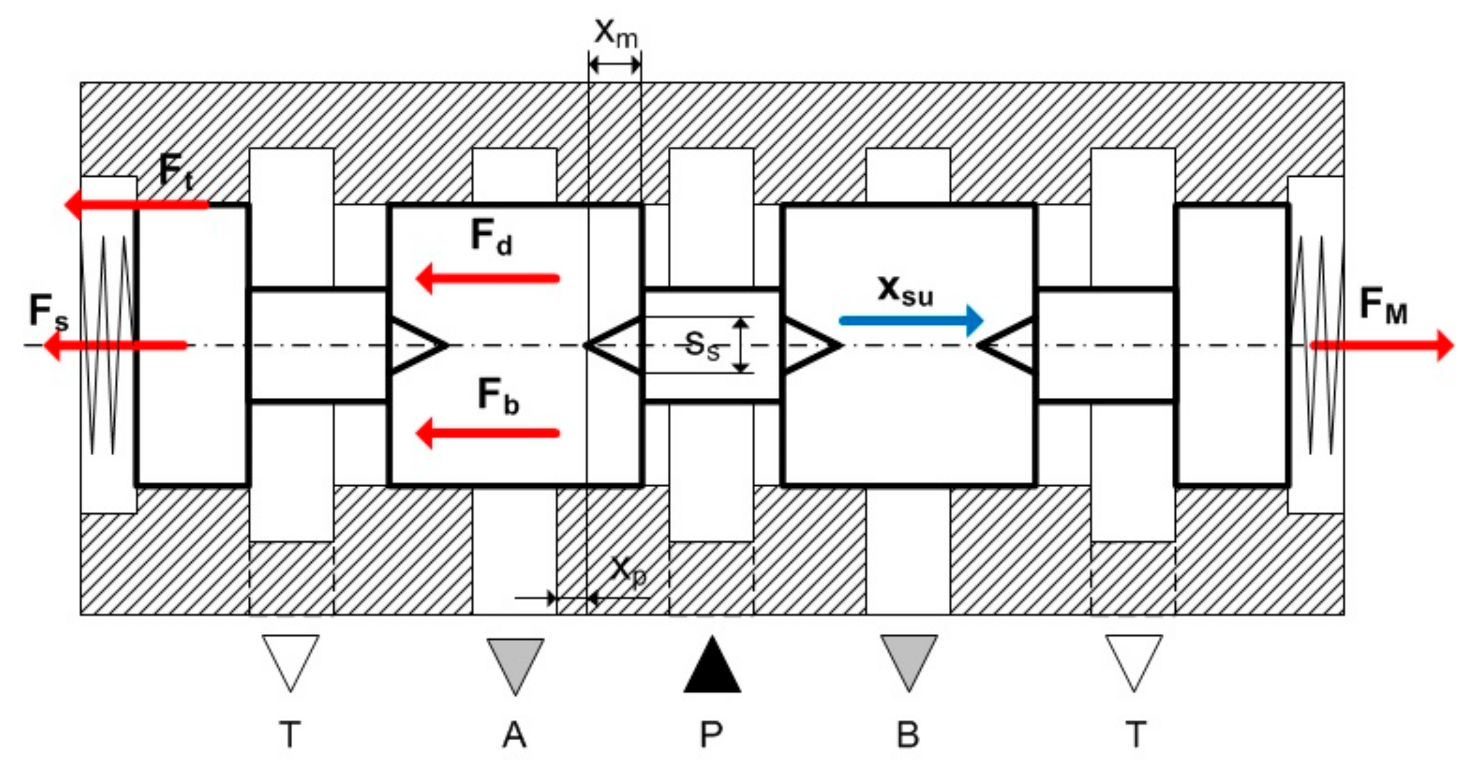
In addition, in order to simplify the mathematical description, it was assumed that the spool is in the neutral position (there is no fluid flow through the directional control valve), it is not loaded by forces caused by static pressure and there are no resistive forces caused by seal friction. When analysing the theoretical model of a spool valve, the balance of forces acting on the spool can be considered as a starting point (Figure 2).

The literature [14] divides forces into transverse and longitudinal, depending on their direction. These forces determine the resistance of the spool movement that must be overcome when shifting the flow direction. Lateral forces caused by the movement of the spool relative to the sleeve have no direct effect, but by acting perpendicularly to the axis of the spool they determine the frictional forces (and, as a result, the resistive forces) on the surface of the spool; these forces have been examined, for example, in [22]. On the other hand, the values of longitudinal loads are often much greater than the values of inertia and the frictional forces acting on the spool; they are therefore decisive when determining the force necessary to shift the valve spool [23].

The forces acting on a moving spool are as follows:

• Spool inertia:

  $$F_b=m_c\frac{d^2{x}_{su}}{d{t}^2},$$

  (10)

  where m_c is the mass of the moving control elements of a piston spool and its associated liquid column (kg) and x_su is the spool displacement (m).
• Stiffness of centring springs:

  $$F_s=c_{sz}\cdot x_{su},$$

  (11)

  where c_sz is the equivalent stiffness of centring springs (N/m).
• Frictional force in the spool pair: the literature [24] indicates that friction in this type of pair is fluid friction due to the presence of an oil film between the spool and the sleeve and can be calculated using the following formula [14]:

  $$F_t=\pi \cdot d_t\cdot \frac{l}{h}\cdot \mu \cdot \frac{d{x}_{su}}{dt},$$

  (12)

  where d_t and l are the piston diameter and length (m) and h is the thickness of the gap in the spool pair (m).

According to [14], Coulomb friction can be disregarded where the spool pair has adequate lubrication. This simplification can lead to large discrepancies among both experimental results and results based on this model for higher spool shifting speeds [25]. Based on tribological considerations [26,27], a more detailed model of friction in the form of mixed friction can be assumed to exist in the spool–sleeve pair.

The forces acting on the spool moving in the sleeve can be calculated using the following formulas—model 1:

$$m_c\frac{d^2{x}_{su}}{d{t}^2}+\pi d_t\frac{l}{h}\mu \left(\frac{d{x}_{su}}{dt}-\frac{dw}{dt}\right)+c_{sz}\left(x_{su}-w\right)+k_t\left(d_{k0}-a_{k0}\right)\delta \left(\frac{d{x}_{su}}{dt}-\frac{dw}{dt}\right)=0,$$

(13)

$$k_t=C_k{\mu }_s,$$

(14)

where w is the amplitude of external excitation (m), µ is the dynamic viscosity of the fluid (Ns/m²), d_k0 and a_k0 are the dimensions of the microwedge (m), k_t is the coefficient of proportionality between the frictional force and the value of contact strain (N/m), C_k is the contact stiffness of the surface (N/m) and µ_s is the coefficient of static friction (-).

The first term of Equation (13) describes the inertia of the spool movement, the mass of the associated fluid and 1/3 of the mass of the springs. The second term describes the fluid frictional force that occurs during the movement of the spool and proportional to its relative speed, while the third term describes the stiffness force from the centring springs, and the fourth term describes the static friction force. The second and last terms of Equation (13) therefore describe the mixed frictional force, which can be written as follows:

$$F_{Tm}=\pi d_t\frac{l}{h}\mu \frac{d{x}_{su}}{dt}+k_t\left(d_{k0}-a_{k0}\right),$$

(15)

The term δ corresponds to the Dirac delta function, which takes the value of 1 when the relative velocity of the spool and sleeve is 0; it otherwise takes the value of 0. This function can be approximated as:

$$\delta \left(\frac{d{x}_{su}}{dt}-\frac{dw}{dt}\right)\approx \frac{1}{1+{10}^{\theta }\cdot {\left(\frac{d{x}_{su}}{dt}-\frac{dw}{dt}\right)}^{\iota }},$$

(16)

The value of exponent θ should be as large as possible (θ >> 1) and the exponent t should take a large value and be an even number (t >> 1 and t = 2 × k_p, where k_p is a positive integer). These requirements are due to the fact that according to the literature [10], the denominator of expression (16) should tend towards infinity when the relative velocity of the spool and sleeve is other than 0.

If there are seals in the spool pair, this must also be taken into consideration in model (13). The frictional force of the seals can be approximated as follows [28,29]:

$$F_{Tu}=\pi \cdot D_p\cdot l_u\cdot f_t\cdot N_k+\pi \cdot D_p\cdot l_{u1}\cdot f_{t1}\cdot p,$$

(17)

where l_u and l_u1 are the width of the sealing surface of the rubber ring and retaining ring (m), f_t and f_t1 are the coefficients of friction of the rubber and retaining ring materials (-) and D_p is the inner diameter of the ring (m).

If there is no retaining ring, the second component of the sum in Equation (17) can be disregarded. The friction coefficient f_t under hydrodynamic lubrication is expressed using the following equation [29]:

$$f_t=c_p\frac{\mu \cdot v}{N_k\cdot h_0},$$

(18)

where c_p is the correction factor (-), N_k is the value of contact pressures (N/m²) and h₀ is the lubricating film thickness (m).

The mixed friction model in the spool–sleeve pair can be presented based on the theory that the mixed friction force is the sum of molecular forces acting in micro-areas of contact and drag forces in the fluid; papers postulating this interpretation include [10,27]:

$$F_{Tm}={\mu }_m\cdot N,$$

(19)

$${\mu }_m=C_1\sqrt{\frac{d{x}_{su}}{dt}-\frac{dw}{dt}}+\frac{C_2}{\frac{d{x}_{su}}{dt}-\frac{dw}{dt}}$$

(20)

To avoid uncertainty when the relative velocity of the spool is zeroed, Equation (21) was modified as follows:

$${\mu }_m=C_1\sqrt{\frac{d{x}_{su}}{dt}-\frac{dw}{dt}}+\frac{C_2}{\frac{d{x}_{su}}{dt}-\frac{dw}{dt}+{\gamma }_m},$$

(21)

where the constant γ_m is near zero. The value was taken to be γ_m = 1 × 10⁻². The value of constant γ_m is consistent with the velocity in m/s. Moreover, μ_m is a dimensionless parameter.

Taking into account (19) and (21), the mixed friction model can therefore be represented as follows:

$$F_{Tm}=\left(C_1\sqrt{\left|\frac{d{x}_{su}}{dt}-\frac{dw}{dt}\right|}+\frac{C_2}{\left|\frac{d{x}_{su}}{dt}-\frac{dw}{dt}\right|+{\gamma }_m}\right)\cdot N,$$

(22)

where C₁ and C₂ are the fixed values of coefficients ($\sqrt{s/m}$) and (s/m), respectively; N is the normal load (N) and γ_m is the higher-order minor value (m/s).

Thus, the model of interaction of the spool–sleeve pair can be presented as follows—model 2:

$$m_c\frac{d^2{x}_{su}}{d{t}^2}+\pi d_t\frac{l}{h}\mu \left(\frac{d{x}_{su}}{dt}-\frac{dw}{dt}\right)+c_{sz}\left(x_{su}-w\right)+\mathit{sgn}\left(\frac{d{x}_{su}}{dt}-\frac{dw}{dt}\right)\cdot \left(C_1\sqrt{\left|\frac{d{x}_{su}}{dt}-\frac{dw}{dt}\right|}+\frac{C_2}{\left|\frac{d{x}_{su}}{dt}-\frac{dw}{dt}\right|+{\gamma }_m}\right)\cdot m_{su}\cdot g=0$$

(23)

The proposed mixed friction model, calculated with Equation (23), describes both situations where the spool is stationary relative to the sleeve and where the components are in relative motion. By introducing the constant γ_m into model (23), it was possible to avoid the value of the frictional force increasing to infinity while the spool is stationary, which does not happen in practice.

The literature [20,30] also describes a mixed friction model derived from Coulomb’s law and hydrodynamic equation:

$$F_{Tm}=F_{Ts}-F_{Tp},$$

(24)

$$F_{Tm}={\mu }_m\cdot N,$$

(25)

$${\mu }_m={\mu }_0-K_V\cdot \frac{\mu }{h}\cdot \frac{v}{p},$$

(26)

therefore:

$$F_{Tm}=\left({\mu }_0-K_V\cdot \frac{\mu }{h}\cdot \frac{v}{p}\right)\cdot N,$$

(27)

where: F_Ts is a force of Coulomb friction (N), F_Tp is a force of fluid friction (N), µ₀ is the dry friction coefficient (-), K_V is a dimensionless coefficient characterising the geometry of contact of friction surfaces, µ is the dynamic fluid viscosity, (N·s/m²), h is the oil film thickness in m, v is the velocity of relative motion of friction surfaces in m/s, and p = N/A_t, A_t is the friction surface area in m².

This model can be introduced into the equation of the balance of forces acting in the spool–sleeve pair during their relative movement—model 3:

$$\begin{array}{c}{m}_c\frac{d^2{x}_{su}}{d{t}^2}+\pi d_t\frac{l}{h}\mu \left(\frac{d{x}_{su}}{dt}-\frac{dw}{dt}\right)+c_{sz}\left(x_{su}-w\right)+\mathit{sgn}\left(\frac{d{x}_{su}}{dt}-\frac{dw}{dt}\right)\\ \cdot \left({\mu }_0-K_V\cdot \frac{\mu }{h}\cdot \frac{\left|\frac{d{x}_{su}}{dt}-\frac{dw}{dt}\right|}{p}\right)\cdot m_{su}\cdot g=0\end{array}$$

(28a)

$$\begin{array}{c}{m}_c\frac{d^2{x}_{su}}{d{t}^2}+\left[\pi d_t\frac{l}{h}\mu -K_V\cdot \frac{\mu }{h}\cdot m_{su}\cdot g\right]\left(\frac{d{x}_{su}}{dt}-\frac{dw}{dt}\right)+c_{sz}\left(x_{su}-w\right)+\\ \mathit{sgn}\left(\frac{d{x}_{su}}{dt}-\frac{dw}{dt}\right)\cdot {\mu }_0\cdot m_{su}\cdot g=0.\end{array}$$

(28b)

On the other hand, if it is assumed that only fluid friction occurs in the spool pair due to good lubrication, the model of the spool oscillating movement can be written as follows—model 4:

$$m_c\frac{d^2{x}_{su}}{d{t}^2}+\pi d_t\frac{l}{h}\mu \left(\frac{d{x}_{su}}{dt}-\frac{dw}{dt}\right)+c_{sz}\left(x_{su}-w\right)=0.$$

(29)

If the oscillating movement of the spool is described using the above model, the spool is bound to the body by centring springs (the second term of the equation) and by fluid friction in the spool pair (the third term of the equation).

Experimental tests were carried out and selected parameters were estimated using specialised software in order to parametrise the equations of the mathematical models presented above.

3. Experimental Tests

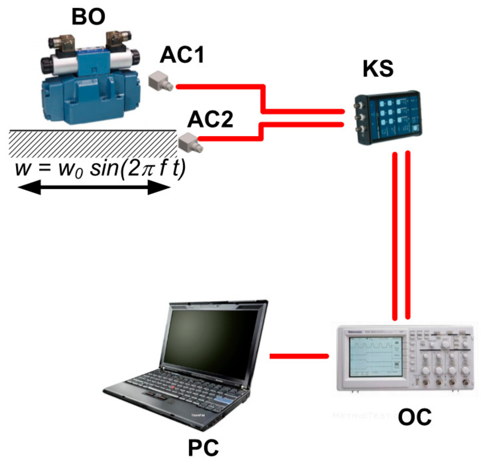
Experimental tests were carried out, where the main stage of a 4/3 4WEH 10 J46/6EG24NETK4/B10 directional control valve manufactured by Bosch-Rexroth was subjected to external mechanical oscillations in a frequency range of 10 to 100 Hz. During the tests, the control chambers of the main stage of the directional control valve were pressure-relieved, i.e., the pressure in the chambers was equal to the atmospheric pressure. The acceleration of the oscillations of the directional control valve spool and the body were recorded.

The tests were carried out on a directional control valve immersed in HL68 or Azolla ZS22 oil at a temperature of 20 °C (with a dynamic viscosity of 612 × 10⁻⁴ or 198 × 10⁻⁴ N·s/m, respectively). The centring spring pair was replaced after each series of tests. The spring stiffness and the oil type are given in

Table 1. Selected parameters of the directional control valve model.

No.	Spring Stiffness—cs (N/m)	Oil Type
1.	816	Azolla ZS22
2.	2923	HL68
3.	2923	Azolla ZS22
4.	816	HL68

. Mechanical oscillations were generated using a Hydropax ZY-25 linear hydrostatic drive simulator. The direction of excitation oscillation was aligned with the direction of movement of the spool in the sleeve.

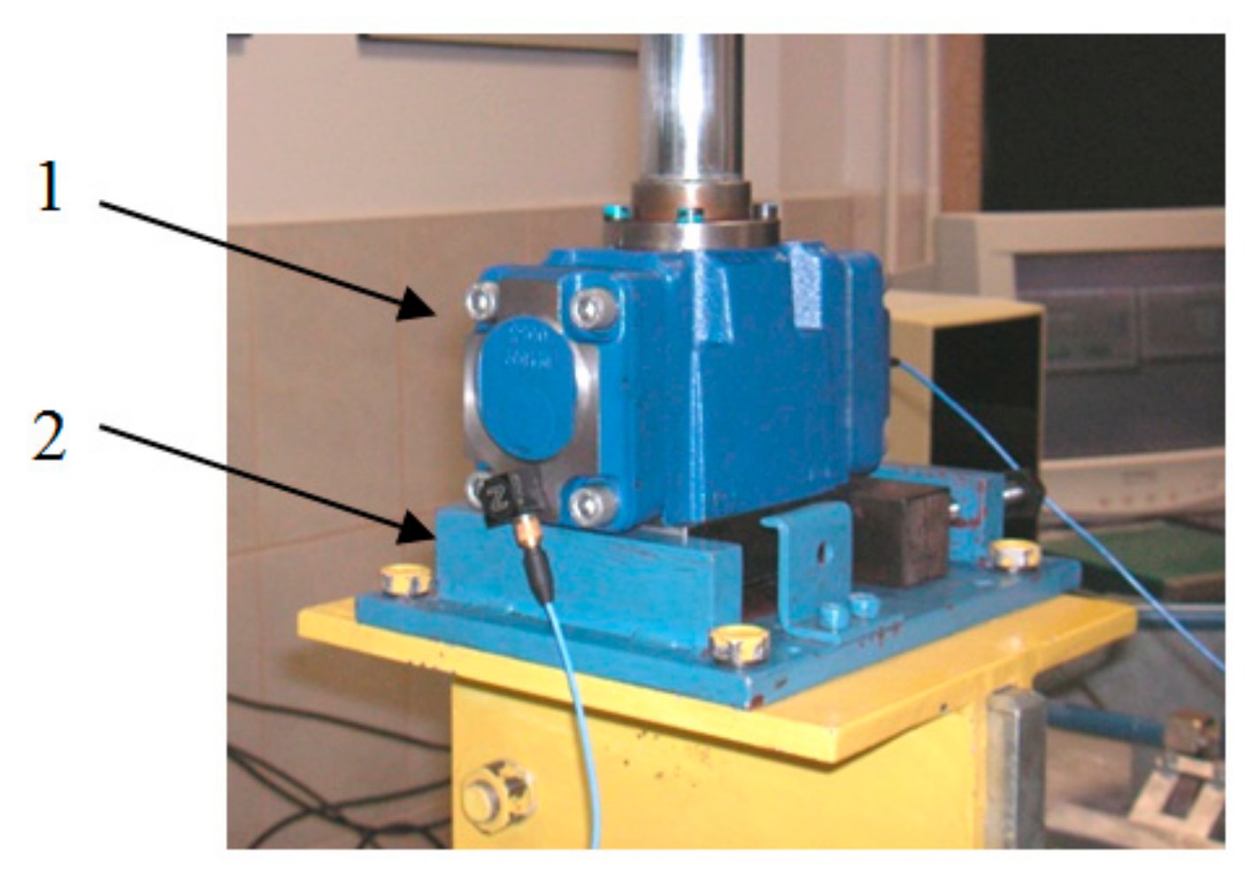
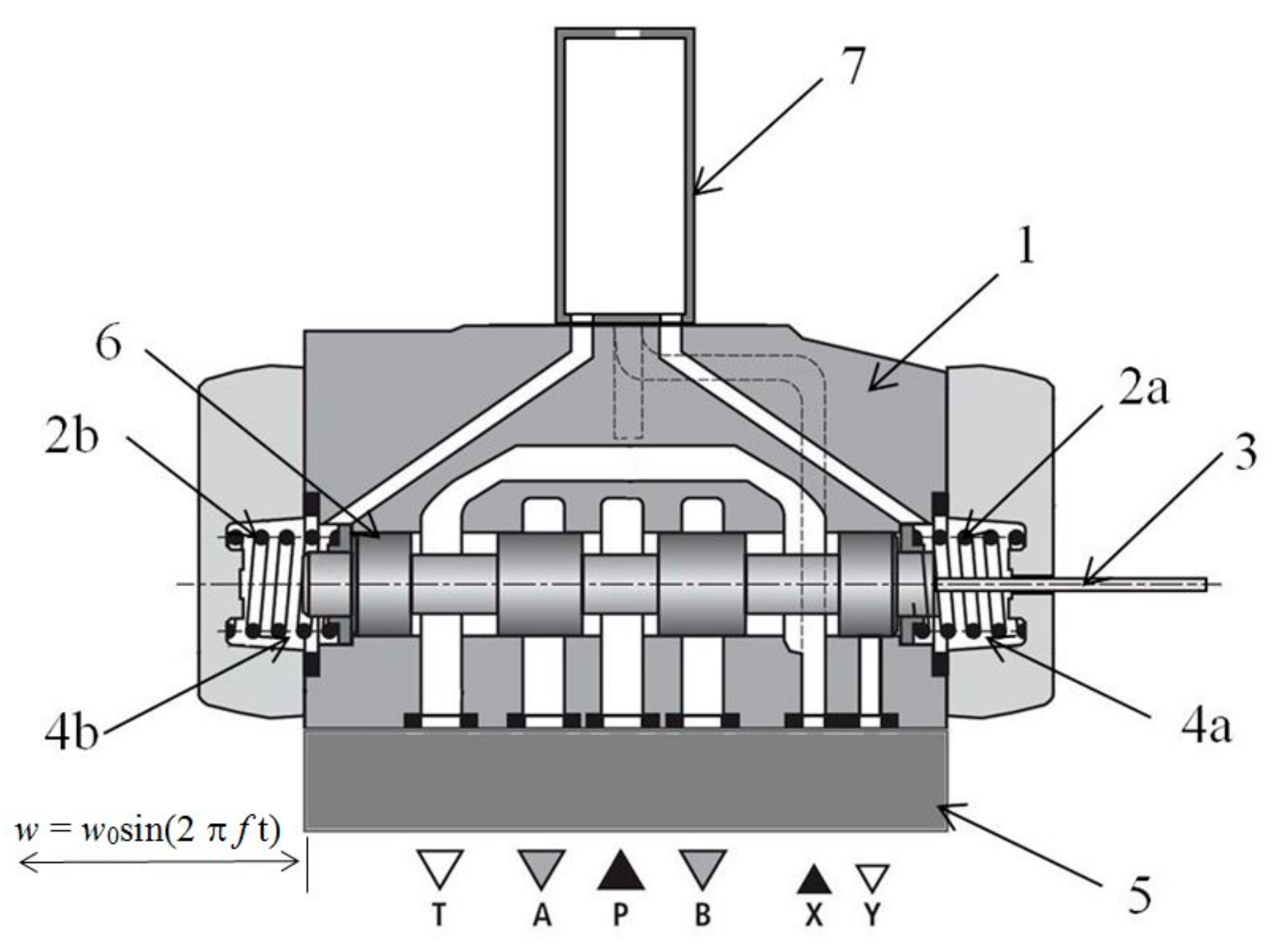
The directional control valve was mounted in a special holder on the simulating table. Figure 3 shows the directional control valve during testing. Figure 4 and Figure 5 show a diagram of the directional control valve and the measurement path.

As shown in Figure 5, two accelerometers were used for the acceleration measurement. AC1 was mounted to the spool while AC2 was mounted to the valve body. The sensor uncertainty δa_acc was equal for both sensors. The signal from the accelerometers a_acc was obtained by a signal conditioner with gain factor K₁ and error of gain δK₁. The signal was then passed to the oscilloscope which further amplified it. The oscilloscope had a gain factor of K₂ with gain error δK₂. From the above, the measured acceleration can be described by the following equation:

a = a_accK₁K₂

(30)

As the measurement uncertainty for each device is different, the acceleration is a function of three variables. The total measurement uncertainty can be presented as follows:

$$\Delta \mathrm{a}=\frac{\partial \mathrm{a}}{\partial {\mathrm{a}}_{\mathrm{acc}}}\Delta {\mathrm{a}}_{\mathrm{acc}}+\frac{\partial \mathrm{a}}{\partial K_1}\Delta K_1+\frac{\partial \mathrm{a}}{\partial K_2}\Delta K_2$$

(31)

The relative uncertainty δa is described by the equation:

$${\mathsf{\delta }\mathrm{a}=\mathsf{\delta }\mathrm{a}}_{\mathrm{acc}}+\mathsf{\delta }{K}_1+\mathsf{\delta }{K}_2$$

(32)

For the measuring apparatus used for the experiment, the relative uncertainty of the acceleration was equal to 5%.

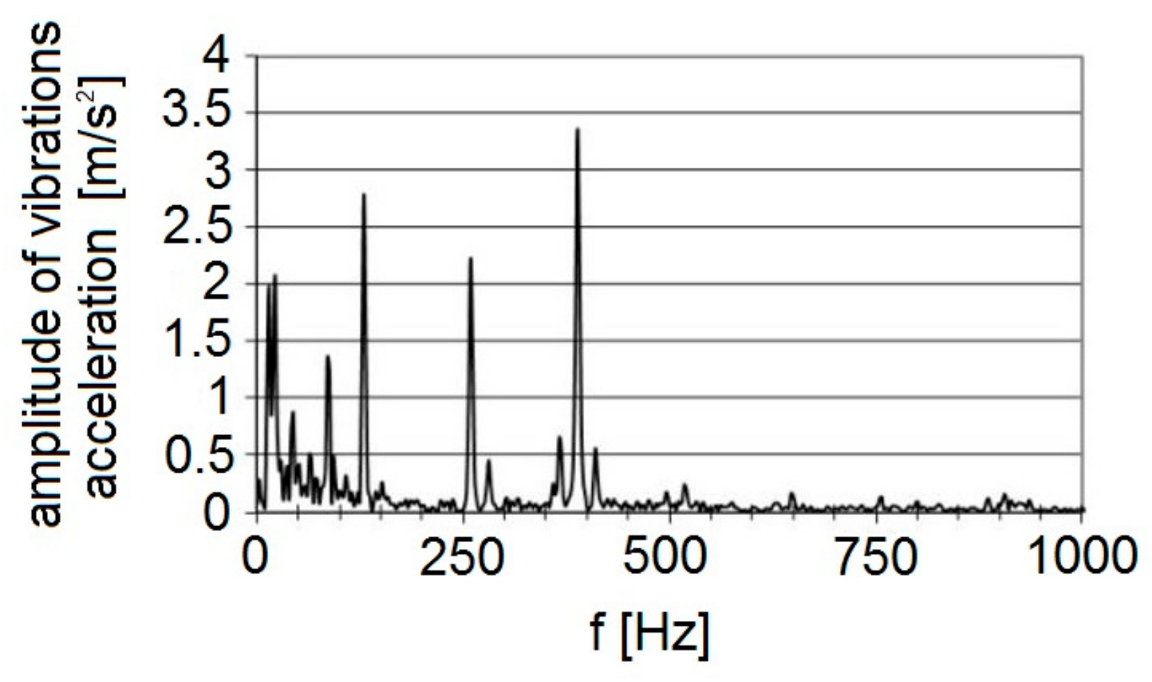
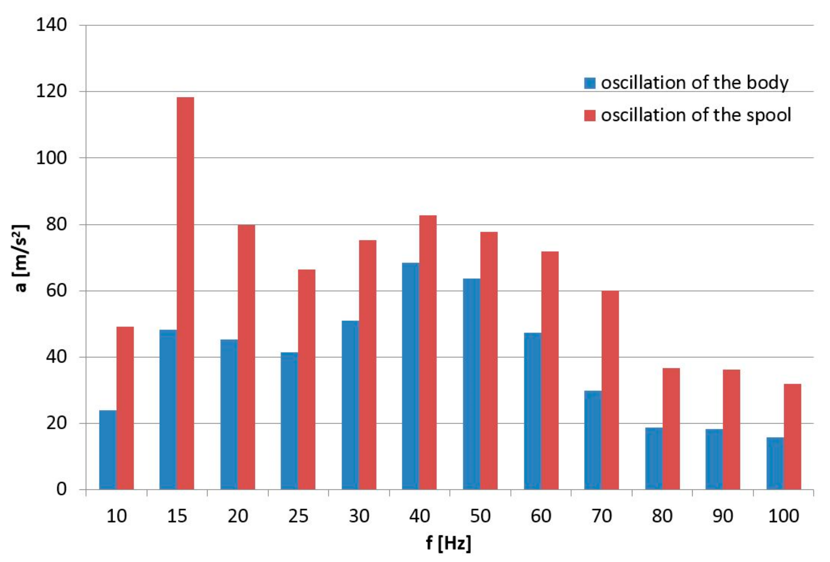
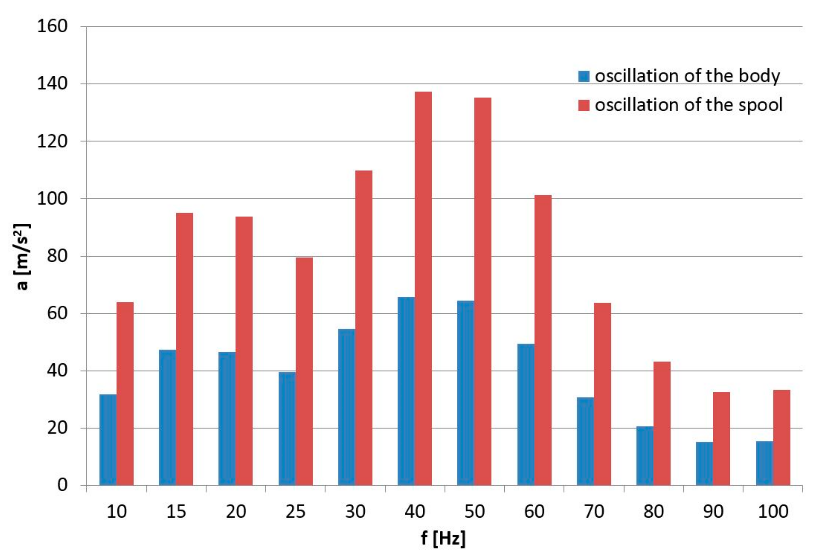
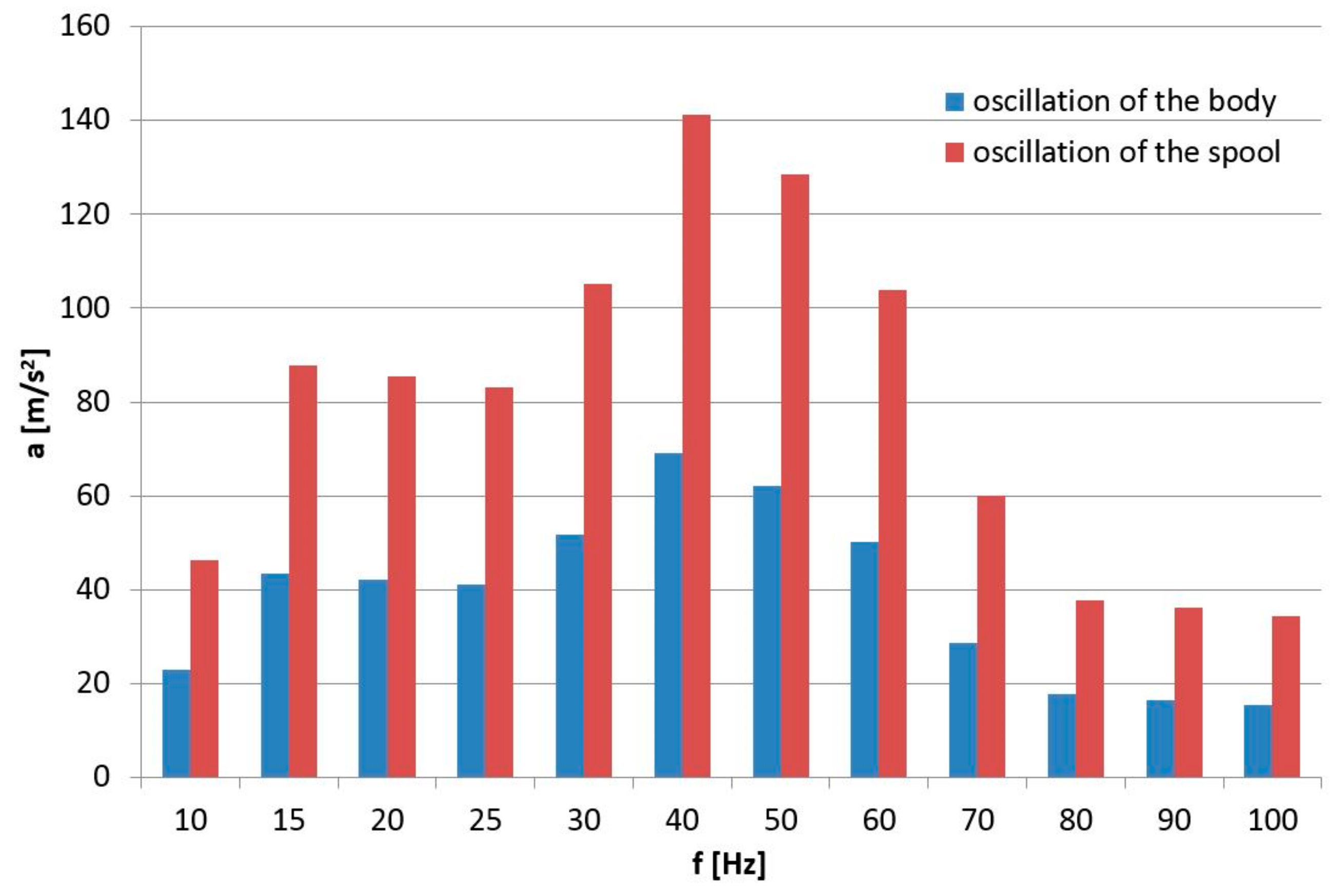
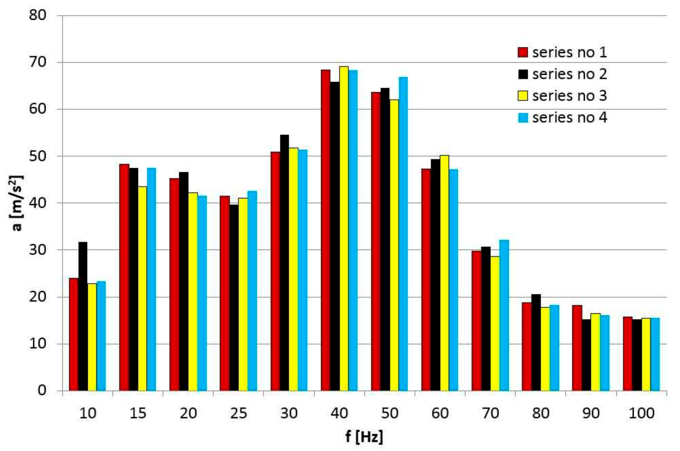
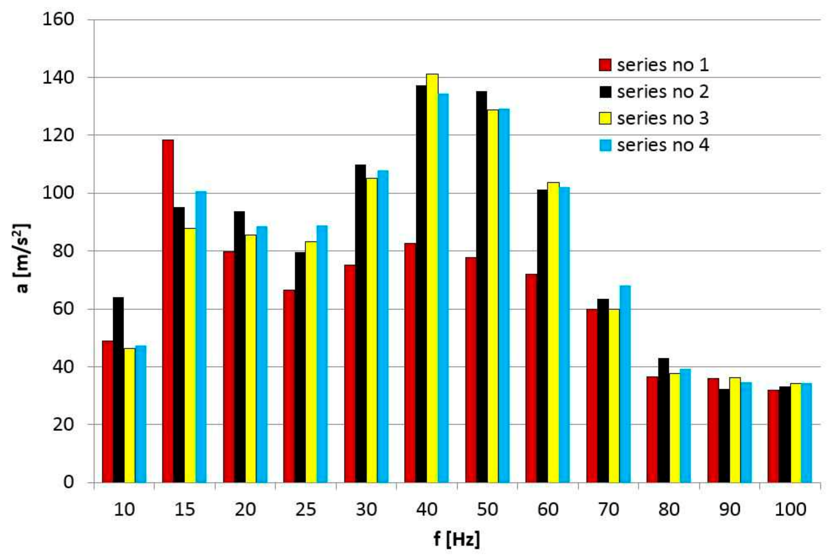
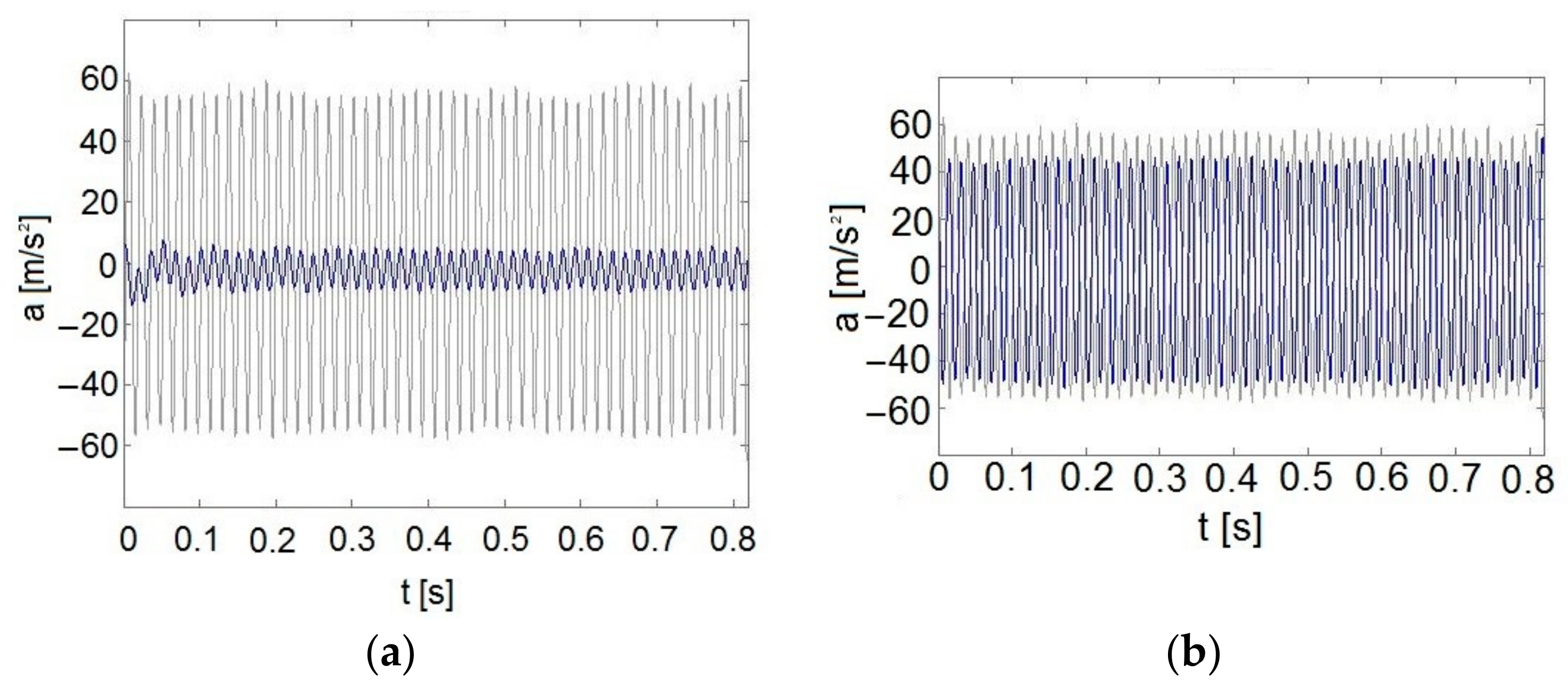
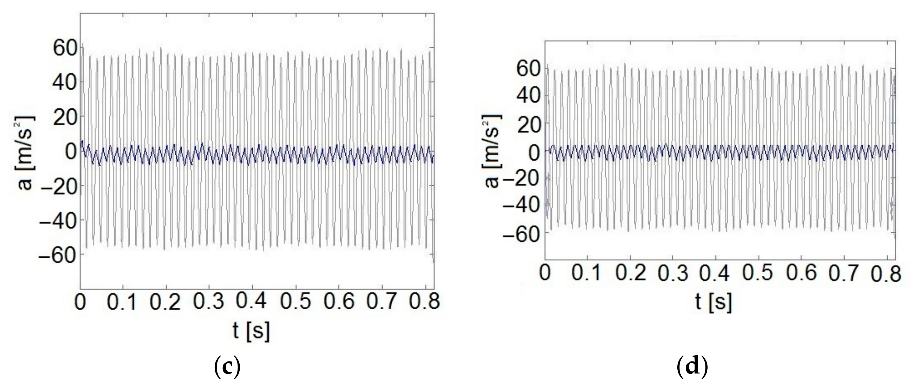
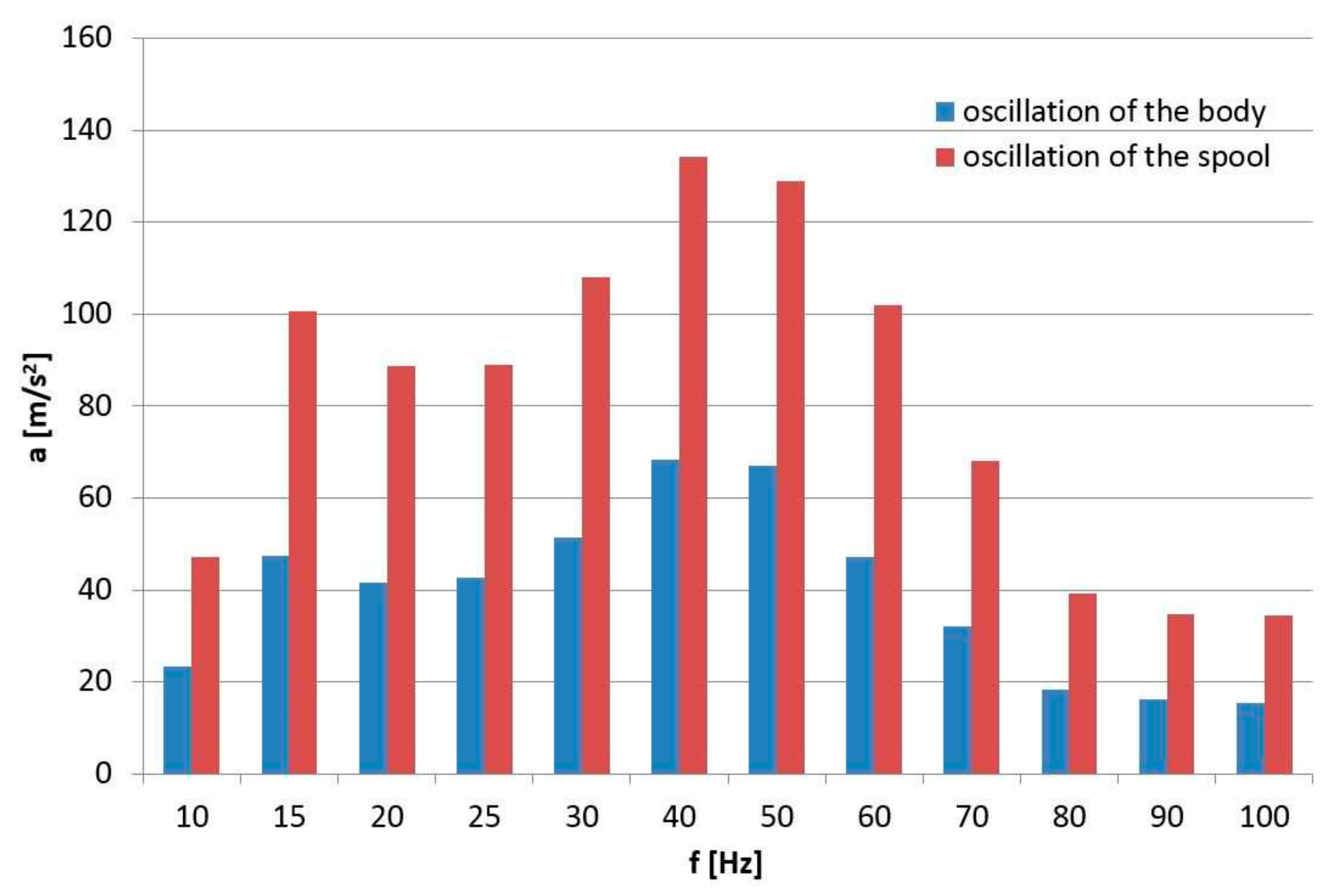
The results of each test are presented individually below (Figure 6, Figure 7, Figure 8 and Figure 9) and then compared (Figure 10 and Figure 11). The amplitudes of oscillation acceleration of the directional control valve body and the spool are compared for a given oscillation frequency of the simulating table used in accordance with the testing scheme.

The results indicate that the oscillation of the spool corresponded to the oscillation of the valve body. The amplitude of oscillation acceleration of the spool was higher in areas where the amplitude of oscillation acceleration of the directional control valve body increased. The undamped natural frequency of oscillation in measurement series 1 and 4 (equivalent spring stiffness: 1632 N/m; mass of spool, lubricant and 1/3 of the mass of the springs: 0.18 kg) was approximately 15 Hz, whereas in measurement series 2 and 3 (equivalent spring stiffness: 5846 N/m; mass of spool, lubricant and 1/3 of the mass of the springs: 0.18 kg) the frequency was approximately 29 Hz.

In Figure 11, series 2 and 3 have a slightly higher amplitude of oscillation acceleration in the resonant area (30 Hz) of the spool in comparison to amplitudes at lower excitation frequencies. There were slight differences in the values of spool oscillation amplitudes when using springs with the same stiffness and oils with different viscosities. However, series 1 (Figure 6) had a notably higher amplitude of acceleration of spool oscillations in the resonant area (15 Hz). In series 4 (Figure 9), this difference was markedly reduced by using a lubricant with a higher dynamic viscosity (HL68 instead of Azolla ZS22, with dynamic viscosities of 612 × 10⁻⁴ and 198 × 10⁻⁴ N·s/mm, respectively).

4. Estimation of the Parameters of Mathematical Models

By performing the experiments and using the Simulink Parameter Estimation tool in the Matlab environment, it was possible to parametrise the models which describe the oscillating movement of the spool, taking mixed friction into account. The major parameters of the spool pair were determined from the authors’ own measurements and from data taken from the literature [14,31] (

Table 2. Selected parameters of the spool pair.

Symbol	Name	Value	Unit
mc	mass of spool + mass of lubricant + 1/3 of the mass of springs	0.18	(kg)
csz	equivalent stiffness of the springs	1632 or 5846	(N/m)
msu	mass of spool	0.172	(kg)
dt	piston diameter	20 × 10−3	(m)
h	radial play in the spool–sleeve system	15 × 10−6	(m)
l	length of the piston	32 × 10−3	(m)
μ	dynamic viscosity of the lubricant (HL68 or Azolla ZS22 at a temperature of 20 °C)	612 × 10−4 or 198 × 10−4	(N*s/m2)

).

Table 3. Values of estimated parameters in model 1.

(Equivalent Stiffness of Springs in N/m, Hydraulic Oil)	ak0 (m)	dk0 (m)	kt (N/m)	Objective Function
(1632, HL68)	0.00356	0.00565	46.86	4.1084 × 107
(5846, HL68)	1.9854 × 10−6	0.00732	100	7.618 × 107
(5846, Azolla ZS22)	2 × 10−6	8 × 10−6	100	1.0015 × 108
(1632, Azolla ZS22)	7.1717 × 10−5	0.0032	99.985	3.1135 × 107

shows the estimated parameters a₀, d₀ and k_t in model 1, described using Equation (13).

Using the same software tool, the parameters in model 2 were estimated and described using Equation (23) (

Table 4. Values of estimated parameters in model 2.

(Equivalent Stiffness of Springs in N/m, Hydraulic Oil)	${\mathrm{C}}_1 \mathbf{\left(}\sqrt{s\mathbf{/}m}\mathbf{\right)}$	C2 (s/m)	Objective Function
(1632, HL68)	10.0536	9.6365	1.67 × 107
(5846, HL68)	9.9998	9.9906	1.81 × 107
(5846, Azolla ZS22)	9.9998	10.0046	1.72 × 107
(1632, Azolla ZS22)	9.9684	15.9903	8.98 × 106

).

Table 5. Values of estimated parameters in model 3.

(Equivalent Stiffness of Springs in N/m, Hydraulic Oil)	µ0	KV	Objective Function
(1632, HL68)	0.16025	0.77652	2.4495 × 107
(5846, HL68)	0.10885	−0.047217	7.4157 × 107
(5846, Azolla ZS22)	0.10039	−0.0008	9.8865 × 107
(1632, Azolla ZS22)	0.03823	0.025445	3.1519 × 107

presents the estimated parameters in model 3, described using Equation (28a).

However, as noted above, if fluid friction is assumed to be the only type of friction in the spool pair, generating the force described by Equation (12), significant differences between the results of a simulation based on this assumption and the results of experimentation will arise. The values of estimated parameters and the corresponding values of the objective function are presented in

Table 6. Values of estimated parameters in model 4.

(Equivalent Stiffness of Springs in N/m, Hydraulic Oil)	h (m)	Objective Function
(1632, HL68)	3.1171 × 10−5	2.5752 × 107
(5846, HL68)	8.4188 × 10−6	2.9586 × 107
(5846, Azolla ZS22)	1.9375 × 10−5	2.2014 × 107
(1632, Azolla ZS22)	8.7237 × 10−5	2.9153 × 107

.

The minimization of the value of the objective function, defined as the weighted sum of squared errors, was used as a criterion to verify the correctness of the test results. The default features of the Simulink Parameter Estimation tool were used to make a mathematical model based on a deterministic approach that included the estimated parameter values [32]:

$${\chi }^2\left(a\right)={{\displaystyle \sum }}_{i=1}^K\left[\frac{y_i-y\left(x_i;a\right)}{{\sigma }_i^2}\right],$$

(33)

where x_i and y_i are the coordinates of the experimental points for x—time and y—acceleration amplitude, σ_i is the standard deviation of y_i, K is the number of points and y(x_i; a) is a fitted curve.

An additional criterion was the ratio between the estimated amplitudes of oscillation acceleration and the experimentally measured values, a_est/a_pom, which should be as close to 1 as possible. The values of the objective function and the ratio a_est/a_pom, averaged for the frequency range of 10–100 Hz, are shown in

Table 7. Mean values of the objective function and ratio with acceleration amplitudes for each model.

	Model 1 (13)	Model 2 (23)	Model 3 (28a)	Model 4 (29)
Objective function	6.27 × 107	1.52 × 107	5.73 × 107	2.66 × 107
aest/apom	0.65	0.89	0.70	0.40

.

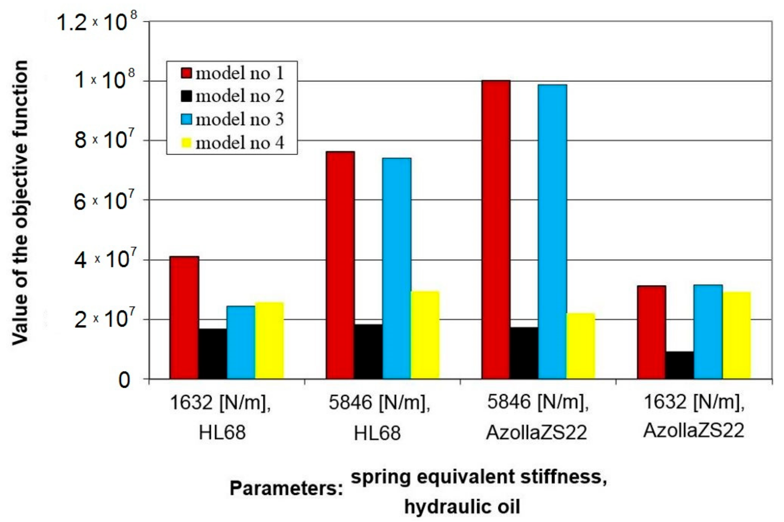
A comparison of the values of the objective function for different equivalent values of stiffness for the springs and hydraulic oils with different viscosities is shown in Figure 12.

A comparison of the time waveforms of the acceleration of spool oscillations among the results of the experiments and the simulations after estimation is presented in Figure 13. The figures show a comparison of the estimated parameters of model 1 (13), model 2 (23), model 3 (28a) and model 4 (29) for the measurement series where equivalent spring stiffness equalled 1632 N/m and the oil used was HL68 oil at a temperature of 20 °C.

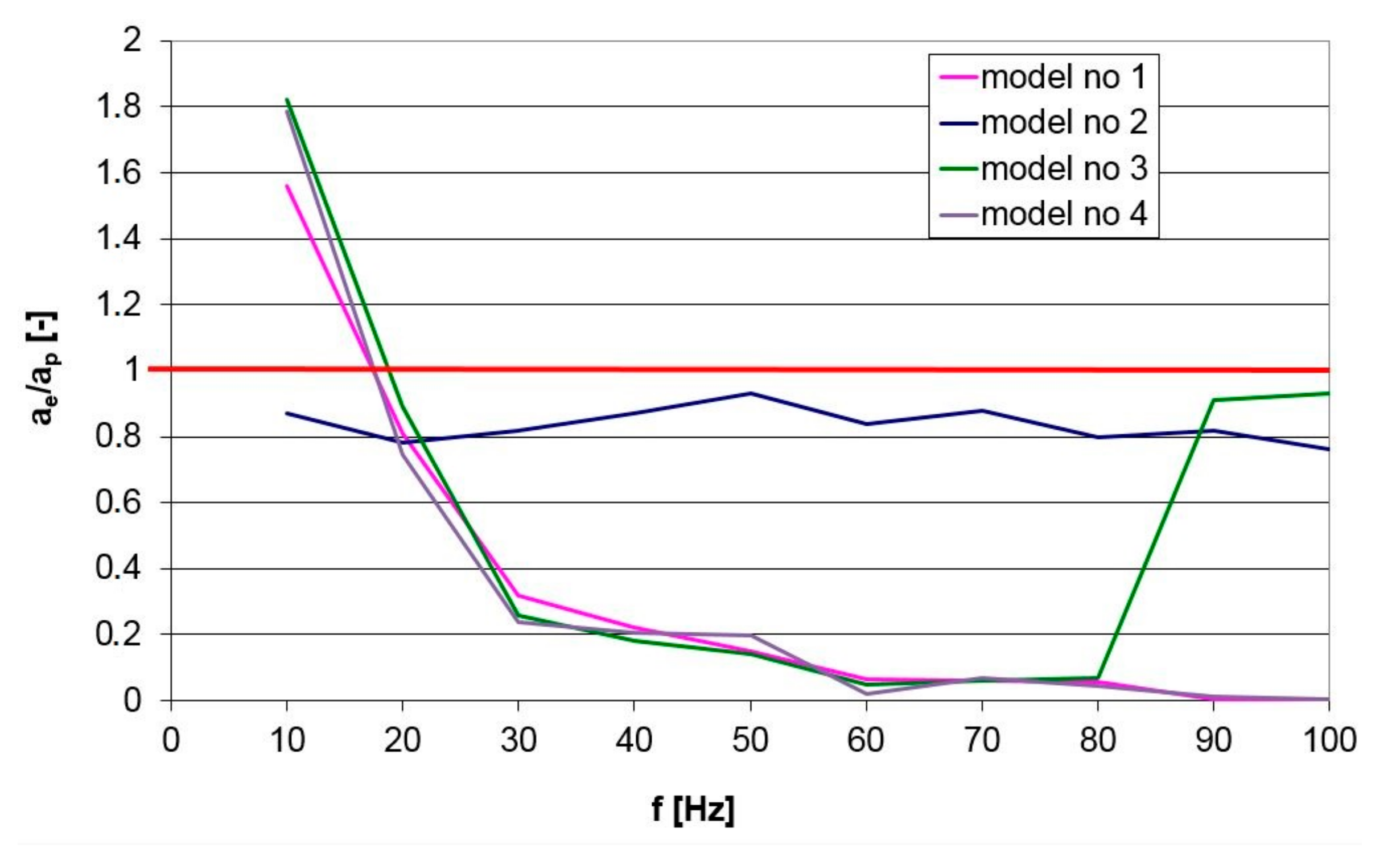
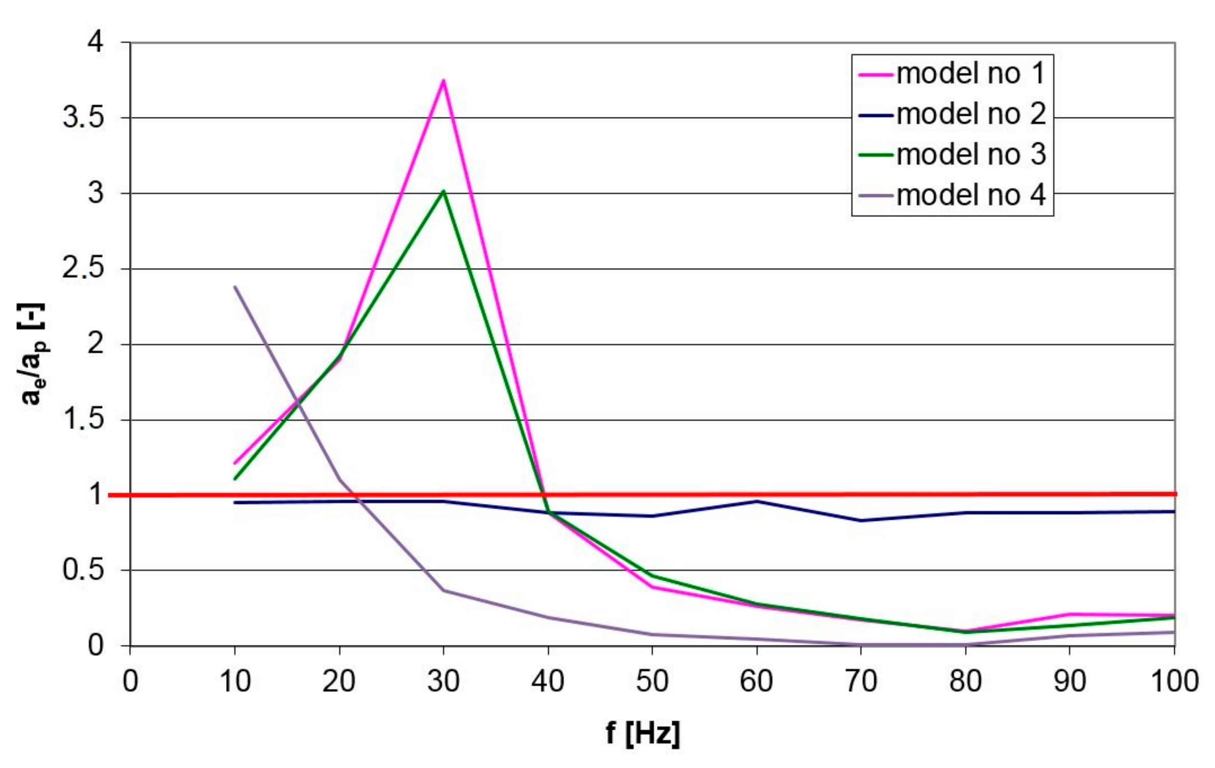
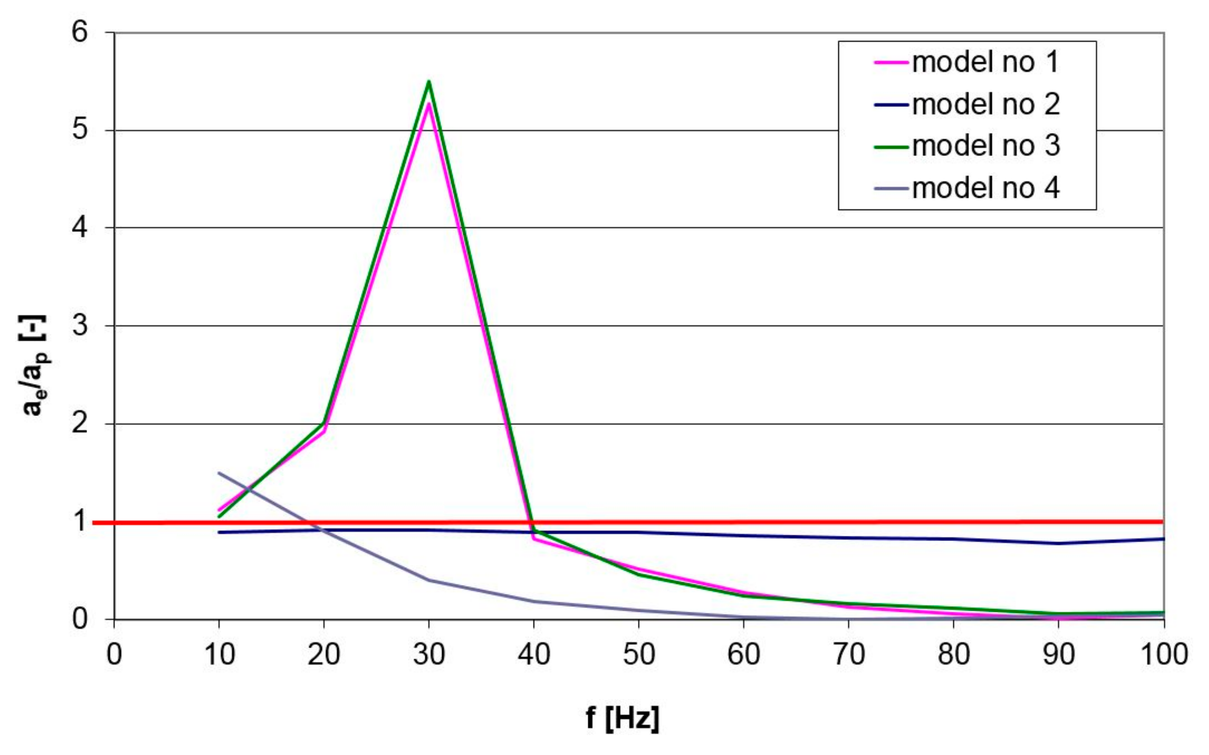
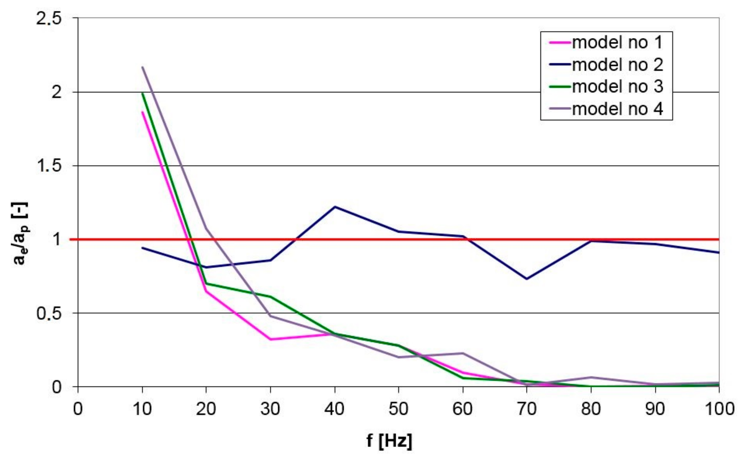
The adequacy of the models for describing the oscillating motion of the spool can be assessed by comparing the amplitudes of acceleration of spool oscillations recorded during testing with the amplitudes calculated from the parametrised model. The ratio of these amplitudes should be as close to 1 as possible. Figure 14, Figure 15, Figure 16 and Figure 17 show this ratio for the different values of centring spring stiffness and the different hydraulic oils used in the testing.

According to the results, after parametrisation and estimation of the constant coefficients C1 and C2, model 2 (23) produced a considerably more accurate description of the oscillation of the spool in the directional control valve sleeve than model 1 (13), model 3 (28a) or model 4 (29) across the entire range of frequencies tested. As seen in Table 7 and Figure 9, for model 2 the averaged value of the objective function was the smallest and the averaged value of the a_est/a_pom ratio was closest to 1. Likewise, the graphs in Figure 14, Figure 15, Figure 16 and Figure 17 indicate that the ratio between the amplitudes of spool oscillation acceleration from the models after estimating the selected parameters and those measured during the tests was closest to 1 when using model 2.

5. Conclusions

This paper analysed the oscillating movement of a hydraulic directional control valve spool. Models of the friction in the spool pair accounted for the kinematic excitation exerted on the body of the directional control valve. Under such conditions, the value of resistive forces generated by the movement of the spool depends on the relative velocity of the spool inside the directional control valve body. It was observed that for higher spool motion speeds (the average spool motion velocity exceeds 0.5 m/s for a spool oscillating at 60 Hz with a full spool stroke of 9 mm), the previously accepted models of linear friction in the spool pair (a fluid friction model) inaccurately represent the oscillating motion. We proposed a model of mixed friction that accounts for the relative motion of the body and the spool. Experimental tests indicated that the proposed model produced a more accurate description of the oscillating movement of the spool (shifting the spool at higher velocities) than the commonly used fluid friction model. In the tests presented in this paper, the vibration amplitude of the valve body was a direct result of the vibration amplitude of the hydraulic vibration exciter—the valve body was non-positively mounted in the holder of the hydraulic vibration exciter. The vibration amplitude of the directional control valve spool is due to the vibration excitation of the valve body and the centring springs used, as well as the viscosity of the hydraulic oil. The use of a set of centring springs with different equivalent stiffnesses changes the value of the natural frequency. The use of hydraulic oil with different viscosities changes the damping in the spool pair and alters the friction conditions of the spool in the directional control valve body. An accurate description of the spool oscillating movement is necessary to assess the effectiveness of any reduction in spool oscillation using passive vibration isolation methods. The reduction in spool vibrations is necessary to reduce pressure pulsations in the hydraulic system caused by the variable area of the directional control valve throttle gaps. This will also contribute to a reduction in vibrations in other components, e.g., hydraulic pipes. The use of a tool for multi-parametric estimation of the coefficients of mathematical models makes it possible, with measured data, to assess the adequacy of different descriptions of the oscillating spool movement.