Analysis of Complexity and Performance for Automated Deployment of a Software Environment into the Cloud

Abstract

Moving to the cloud is a topic that tends to be present in all enterprises that have digitalized their activities. This includes the need to work with software environments specific to various business domains, accessed as services supported by various cloud providers. Besides provisioning, other important issues to be considered for cloud services are complexity and performance. This paper evaluates the processes to be followed for the deployment of such a software environment in the cloud and compares the manual and automated methods in terms of complexity. We consider several metrics that address multiple concerns: the multitude of independent paths, the capability to distinguish small changes in the process structure, plus the complexity of the human tasks, for which specific metrics are proposed. We thus show that the manual deployment process is from two to seven times more complex than the automatic one, depending on the metrics applied. This proves the importance of automation for making such a service more accessible to enterprises, regardless of their level of technical know-how in cloud computing. In addition, the performance is tested for an example of an environment and the possibilities to extend to multicloud are discussed.

1. Introduction

In many business domains, it is beneficial to work with a cloud-based solution, which is easier to maintain than on-premises implementations. Advantages such as disaster recovery, collaboration, and cost savings have attracted many enterprises to adopt such a service-oriented approach, and some of them moved their entire activities to a public cloud [1]. Cloud deployments are known to absolve users from completing tedious maintenance and resource allocation tasks [2]. Beyond this, to support all that is necessary for an application, including infrastructure, data, and development tools, one can adopt an Environment as a Service (EaaS). Such a solution is potentially multicloud, needs automation for the deployment and configuration of the environment, and has to manage resource consumption.

Environment as a Service is an extension of Infrastructure as a Service (IaaS) because it is based on the hardware and the software used in an IaaS system (hypervisors; operating systems; management software; monitoring, and accounting software). Supplementary, EaaS also includes the code and the settings required to run one or more applications (services) in an isolated environment (the isolation provided by container technology). In EaaS, the application and the environment, i.e., the libraries and the runtime, are executed together in a container and can be administered using version control; due to this execution and administering mode, one can automate the applications’ configuration and deployment.

Due to the automation facility, EaaS can be used successfully to deploy test environments, staging environments (to test a production environment), demos (proof of concepts), and online training (the EaaS model being scalable). The EaaS model brings a set of benefits: reducing the costs (for application support and maintenance), rapid application development and deployment (faster results), efficient resource utilization, low cycle time for projects, and flexibility (the changes to an application can be done and applied easily).

Despite these maintenance advantages, when initiating the use of cloud resources, there may be processes to be followed that have many manual tasks and require specialized knowledge to be executed. This stands in the way of a much larger adoption of this kind of service provisioning. For example, the complexity of high-performance computing (HPC) workflows is analyzed in [3]. Li et al. model and analyze the workflows for the auto-scaling scheduler, the job management, and the metering management, and propose a containerized cloud platform to reduce their complexity and assist their users and administrators. The deployment of such a platform remains a challenging task. Apart from complexity, it is also important to attentively monitor the performance of such services for virtual machines and containers, based on standard benchmarks or in regard to what is offered by the native hardware [4]. Bystrov et al. evaluate communication- and computation-intensive services on virtual cloud resources, whose performance depends on MPI communication, load mapping, and overhead [5].

Our research is focused on the automated deployment of a software environment on one or multiple clouds, to deliver support to users with limited technical know-how in cloud computing. Thus, they may be assisted to perform the deployment in a cloud of their choice and destroy the environment when no longer needed. The objective is to determine how much value would be brought to the users by a platform that automates the cloud deployment process, in comparison with the manual methods applied otherwise. This would support the deployment in the cloud of a software environment whenever needed and its delivery as a service.

To assess the proposed automation, the manual deployment process is compared with the automated one from the perspective of the user interaction and the prerequisites required for the manual tasks. We use existing software and process complexity metrics, and we also propose a specific way to evaluate the complexity of human tasks for cloud deployment. The question is how big the differences in complexity are between the manual and the automated deployments, such as to motivate the development or the acquisition of a platform to automate most of the tasks. This would allow a specialist in the application domain to adopt the EaaS approach even without specific knowledge and know-how in cloud computing. Furthermore, by comparing the two deployment processes, one can decide which type of deployment to use, depending on the complexity of the tasks involved and the complexity of the software solution (microservices) to be implemented. Thus, depending on this complexity, the customization of the automatic deployment system may sometimes be much more costly than a manual deployment.

The complexity is considered very important in software because it increases the initial development costs, as well as the ones for maintenance, and it enlarges the risk to generate human or software errors. To assess the complexity of the software environment deployment in the cloud, we model the processes for manual and automated deployment, and we apply the following metrics to them:

-

cyclomatic complexity [6]—A consecrated software metric that considers a program as a graph, hence it may also be calculated for process models; a low value means that the program graph is easy to understand and modify,

-

Yaqin complexity metrics [7]—A set of metrics to assess business process complexity based on basic control structure, and

-

complexity of human tasks—A metric introduced in this paper, which assigns a weight to each process task with respect to how much specific technical knowledge and experience are necessary for performing the task.

Nonetheless, the performance of the resulted service is also important to the adoption of such a solution, and CPU and memory consumption monitoring is also necessary. We need to monitor the performance of a software environment deployed on a Kubernetes cluster and evaluate the automation method from the perspective of the users’ interaction with the platform and of the prerequisites required during the manual deployment. The paper is focused on the IBM Cloud, but it also shows the differences required to ensure the deployment to other clouds and obtain a multicloud deployment platform.

Further on, in Section 2 we present the related work about the deployment in the cloud, as well as the complexity and performance issues. In Section 3 we explain the research method, including models for manual and automated deployment processes, complexity metrics for their analysis, and the choice of tools to monitor the performance of the deployed software environment. The configuration realized for the testing environment is described in Section 3.4. Section 4 shows the results for cyclomatic complexity, Yaqin complexity metrics, and complexity of human tasks. We then give the performance test results obtained with Prometheus and Grafana and Sysdig. Section 5 discusses the comparative complexities of the two processes and analyzes the performance, then briefly presents the automated deployment platform developed as a continuation of this work.

2. Related Work

In Section 2.1, we present related work in regard to cloud deployment in general, with a focus on multicloud. Besides provisioning, when discussing cloud software services, other problems of interest are complexity and performance, hence they are also considered subsequently in Section 2.2 and Section 2.3, respectively.

2.1. Cloud Deployment

Nowadays, when most IT companies use cloud architecture services, most research activities have focused on the IaaS layer, neglecting the rest of the cloud stack [8]. For example, Ferrer et al. present two approaches for PaaS: ASCETiC and SeaClouds [8]. There are multiple solutions, starting with IaaS, PaaS, and SaaS but there are also applications and architectures developed for multicloud. Rani et al. explore different service models and different types of clouds [9], with an emphasis on InterCloud architecture, topologies, and types; InterCloud is a cloud of clouds, interconnecting the infrastructures of multiple cloud providers. There are two types of InterClouds: federation clouds, where the cloud providers are voluntarily collaborating in order to share resources, and multiclouds, where there is no voluntary collaboration between cloud providers and the management of resources, provisioning and scheduling is entirely the responsibility of the client. The multicloud architecture is used to offer any type of cloud service, most of the latest implementations and solutions being oriented on software services (SaaS) including modeling services [10].

The challenges regarding multicloud systems are related to the deployment of the services. Having an architecture composed of multiple cloud systems makes the deployment process much more complex and different from platform to platform. Nonetheless, the deployment process can be different based on the specific application: enterprise-based services [11] or manufacturing services [12]. In order to solve the deployment problem, some research directions have been focused on the integration of third-party cloud platforms and services, and on the development of multicloud interfaces [13,14]. The problem of modeling the optimal and automatic deployment of cloud applications was investigated in [15]. This was done by analyzing the specification of the computing resources required by the software application but also required by the executing environment, the description of deployment rules, and the computation of an optimal deployment to minimize the total cost.

Most of the implementations for multicloud software services are based on container technologies like Docker [16] and OpenShift [17]. A set of tools has also been developed to automate the creation of software services, with one example being Source to Image (S2I), which is an open-source project that aims to automate the creation of container images directly from the source code of the application. S2I creates a container image that is populated with all the requirements of the application, the application is then compiled and deployed into the container without the programmer’s intervention.

2.2. Complexity

From the point of view of complexity, Muketha et al. describe the complexity metrics that can be found in the specialty literature in the last five years and study how a process can be maintained at a lower complexity to be able to keep it as simple as possible [18]. The authors describe the business process modeling languages that are usually used by different organizations to be competitive, such as the business process execution language, showing the reason behind the business transaction. Muketha et al. state that metrics can give us a view of the ability of the software to work properly and identify the level of success or failure. The first is the Cardoso metrics, such as the control flow complexity, which is similar to the cyclomatic complexity, but with differentiated semantics of nodes. Then, there is the interface complexity, which is based on incoming and outgoing data flows. Another one is the Vaderfeesten metric (cross-connectivity metric) based on cognitive complexity; this type of metric is used for error prediction. The idea behind this metric is that, if a process model has high cross connectivity, it is not vulnerable to a high number of errors.

Yaqin et al. propose a new formula that calculates the complexity of a business process model [7]. The Yaqin metric is a sum of other complexity metrics, based on AND, OR, XOR branch complexities, cyclic complexity, depth complexity, etc. The authors applied this formula to different business processes and conducted various experiments to validate it and find its effectiveness. The Yaqin formula returns a higher value if the model is more complex. As a result, the authors state that the complexity metric increases based on the number of elements of the business process. Based on the result, they conclude that this metric is proved to be more sensitive and precise due to the multitude of parameters involved.

A classical metric that is also relevant to our study is cyclomatic complexity, which is widely used by software developers. However, Shepperd notices the insensitiveness of the metric with linear sequences of statements [6] and, as a result, cyclomatic complexity has the value 1 for a linear sequence of any length. Another problem regarding this metric is the inconsistency when used for modularized software; no other aspects of modularity are considered but the addition of extra modules and duplicate code. Ikerionwu uses the equations of the cyclomatic complexity and applies them to different flow graphs obtained from simple programs’ source code to calculate their complexity [19]. The intention is to navigate all the parts of the program at least one time during the execution of the test. The conclusion is that the absence of cohesion implies a high level of complexity.

Dijkman et al. describe similarity metrics that find node matching by comparing labels and attributes of the process, structural similarity, and behavior similarity [20]. These metrics are used by companies that have repositories of more than five hundred process models. The authors identify the need for a search technique that can check if a new model is similar to the ones that are already present in the repositories. They also make the difference between syntactic and structural similarities alongside a practical example. Cardoso et al. also review existing methods for measuring complexity [21]. The complexity of a process determines the probability of an error, so there is a clear need for a quantitative indication of program complexity. This is similar for software and for a business process, as the latter is the enablement of the former. An aspect that also matters is the semantics, which may be different from one process graph to another. Cardoso et al. state that such metrics have advantages such as not requiring rigorous analysis of the process, identifying errors, and reducing the effort to maintain the process.

There is also scientific literature in regard to the assignment of weights to a task for businesses process computation. According to [22], this idea is behind the cognitive functional size (CFS) proposed by Shao and Wang in 2003 [23]. CFS is computed by applying weights between 1 and 4 to control flows. The weights are assigned to the parallel structure, the sequences, the branches, etc. A modification of CFS named cognitive weight, proposed by Gruhn and Laue [24], is also used in [7] to compute the Yaqin metric.

2.3. Performance

From the point of view of performance, a set of metrics are defined at the following levels [25]: monitor—where the performance of the whole system can be watched; analyzer—where one can make performance predictions based on the monitored parameters; planner—where the optimization decision is announced, like virtual machine (VM) placement or migration; and executor—where the orchestration actions are performed. The performance metrics at the monitor level are directly measured and provided by the hardware or the hypervisor. At the analyzer level, the metrics are based on a series of observations that can be analyzed by cognitive engines; a set of such workload parameters are presented in [26]. The metrics used at the planning and execution levels are used to measure the performance of the decision and execution systems of the cloud infrastructure. Another set of performance metrics is composed of three basic metrics for quantifying performance isolation [27]: metrics based on QoS impact, significant points, and integral metrics.

Ahmad et al. describe the performance and scalability metrics for software that resides in the cloud [28]. The platforms used for testing are Amazon and Microsoft Azure. The comparison is made to two cloud software with the same purpose on different platforms and two different cloud offerings on the same platform. Two metrics are described: scalability and elasticity. Besides performance, cost measurements also have a role in the final metric computation. Scalability is defined by the addition of another instance if needed at runtime; it represents the ability to manage the changes when required. The first conclusion presented in [28] is that the required volume of service scales up linearly when the demand grows. The deficiency is met if the demand is larger than the ability to scale in time. First, one calculates the ratio for the ideal instances based on the demand, then one measures the response time of the service for a corresponding demand level. The ideal time for response is approximated. The testing is done by comparing the scalability of VM’s provision in AWS and Microsoft Azure. The scaling is made when the CPU utilization passes 80%. The demand that is done on both VMs that run a web app is done 20 times, in 640 tests on which one calculates the response time for scalability. The result is quite surprising, as the average response times vary on both cloud platforms. In multiple scenarios, one of the cloud platforms came on top in terms of volume scaling performance.

3. Research Method

The manual and automated deployment processes are modeled in Section 3.1 and analyzed, first based on complexity metrics presented in the scientific literature and then with the complexity of human tasks, a specific metric defined for the scope of our work (Section 3.2). Afterward, the performance of the automated deployment process is analyzed dynamically, based on the monitoring tools described in Section 3.3 and the environment configuration from Section 3.4.

3.1. Process Modelling

For the comparison needed in our research, we model both the manual and the automated processes as activity diagrams in Unified Modeling Language. These representations are subsequently used for applying various process complexity metrics and performing the analysis of the two methods statically. The process models are specific to IBM Cloud.

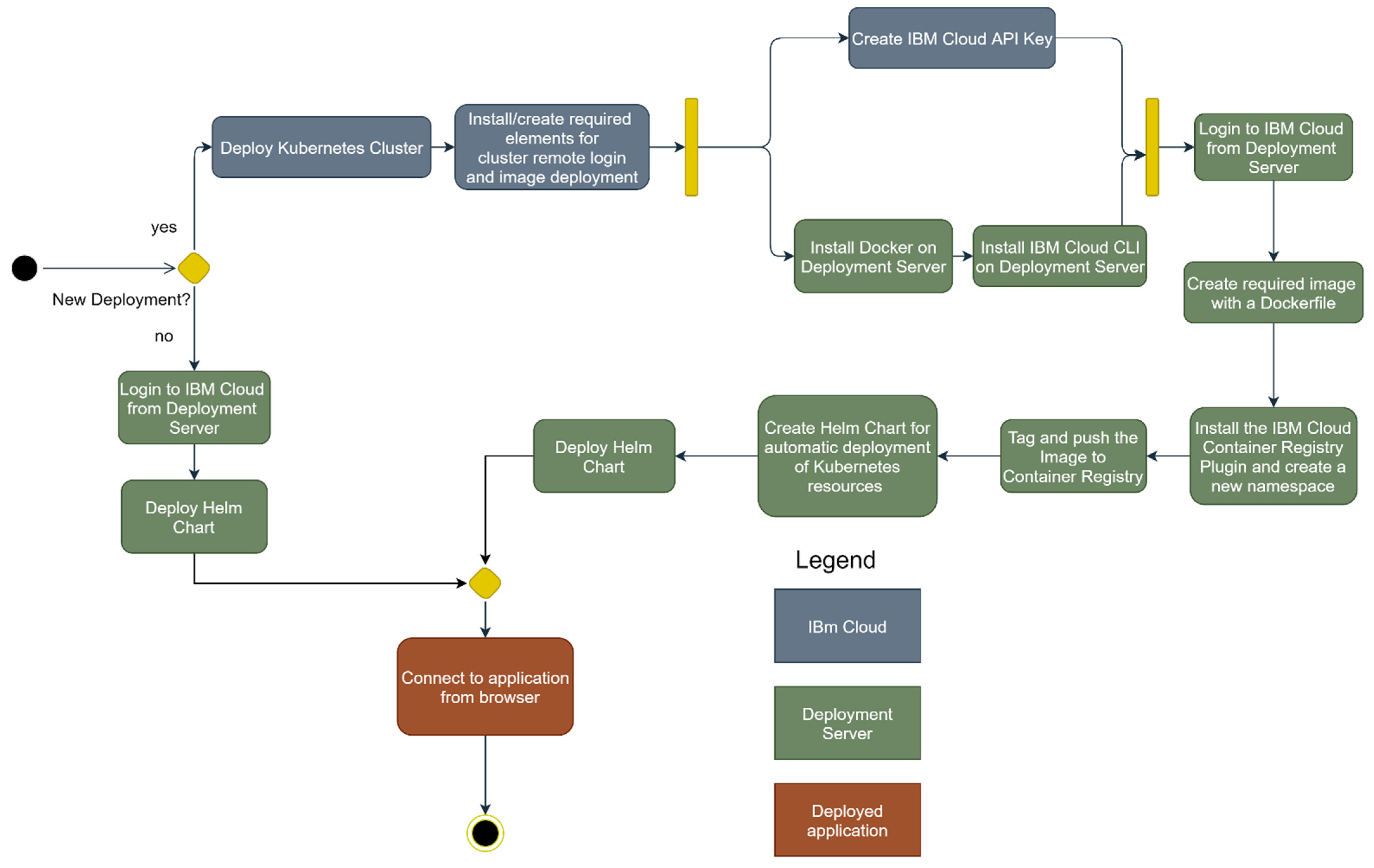
Manual deployment. We first model the deployment process of a software environment in IBM Cloud and represent it in UML (Figure 1). The process starts with the deployment of the Kubernetes cluster—if it is a new deployment—and continues with the establishment of prerequisites for a deployment server. The prerequisites imply the creation of the API key (on the IBM Cloud), and the installation of Docker and IBM Cloud CLI on the deployment server. After that, the user needs to login into the IBM Cloud workspace from the deployment server. Next, the user creates an image for the software environment; this image is based on a Dockerfile that needs to be configured. The configuration tasks continue with the installation of the IBM Cloud container registry plugin, useful for connecting to this component, and a namespace has to be created. The namespace has the role to group the deployed Kubernetes resources. After that, the image is pushed to the IBM Cloud container registry. The next steps consist of the creation of the deployment and the services, which are automatically deployed on the Kubernetes cluster. The process ends with the connection to the newly deployed environment.

If the perquisites are already available and this is not a new deployment, the process is simpler. The user only needs to log in to the IBM Cloud account and deploy the Helm charts that are already created. With the help of the Helm charts, the user can also destroy the environment at will. This makes the deploy/destroy action very accessible. However, such a process needs advanced technical knowledge and know-how for these technologies, and it is also very costly from a time perspective.

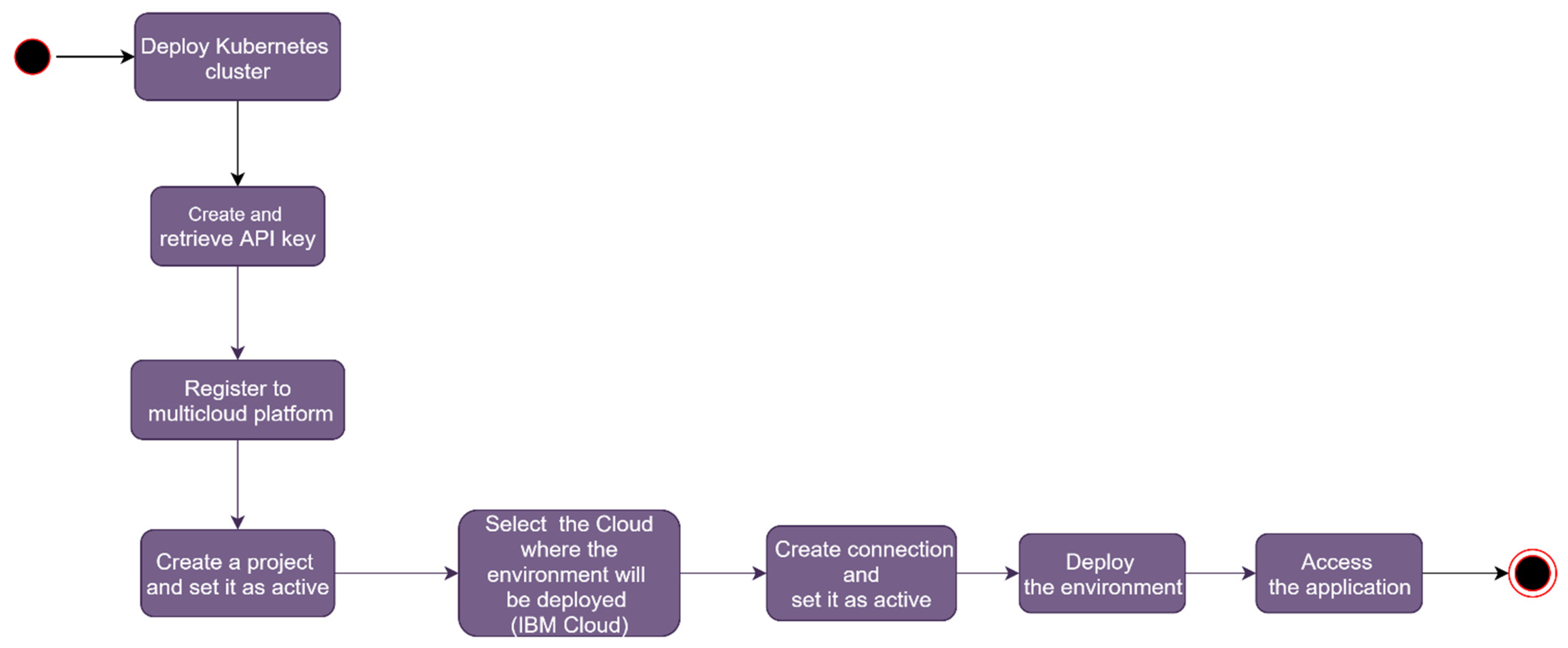
Automated deployment. Using a deployment platform simplifies the users’ work that needs to be done (see Figure 2). In this case, the user still has to deploy the Kubernetes cluster, but this can be done very easily from the IBM Cloud web console. The user also needs to create and retrieve an API key, and this task differs from one cloud provider to another because the connection to the Kubernetes cluster requires other means that are specific to the cloud provider. In the case of IBM Cloud, only an API key needs to be provided by the user at this specific step. The user needs to register to the platform after the Kubernetes cluster is deployed and the API key is retrieved. One should then create a project that has the ability to add users, sensors, and connections. This user can have many projects, so the current project in use must be set as active. Then, the user selects to which cloud he/she wants to connect; the current option is IBM Cloud. After these selections, the user is prompted to add the connection requirements; in this example, the user is required to provide the API key retrieved at the prior step and the Kubernetes cluster name. After that, the user sets the connection as active because, as in the project case, a user can have multiple connections to multiple Kubernetes clusters that reside in multiple clouds that may be supported. The final step is represented by the deployment of the application and by the connection of the user to it.

In comparison with the steps that a user undertakes according to the previously presented manual method, in this case, the advanced technical knowledge that is required for the configuration part is not needed and the deployment is done automatically from the cluster. Practically, the user only interacts with the user-friendly interface of the cloud provider and the multi-cloud deployment platform. The deployment server is practically inexistent for the user and all the tasks are handled by the backend of the application.

3.2. Complexity Metrics for the Deployment Process Analysis

First, we use a classic metric, cyclomatic complexity [6], for the complexity computation of the deployment processes. Cyclomatic complexity, introduced by Thomas McCabe in 1976, determines the complexity of the program using the following equation:

$$v\left(g\right)=e-n+2p$$

(1)

where $v\left(g\right)$ is the complexity of a graph, e is the number of edges, n is the number of nodes and p is the number of exit points. This value generally indicates the effort needed to implement and test the software, as well as the expected error rate. If the value is lower, the number of encountered errors is lower than for a higher value of the cyclomatic complexity.

Second, we apply the Yaqin complexity formula, based on a series of metrics that are calculated for each component of the process seen as a graph [2]:

$$\mathit{YC}=\mathit{Ns}+\mathit{As}+C_{\mathit{AND}}{+C}_{\mathit{OR}}{+C}_{\mathit{XOR}}{+C}_{\mathit{CYC}}{+C}_D$$

(2)

where Ns is the number of nodes, As is the arc size (number of arcs), $C_{\mathit{AND}}$ is the AND branch complexity, $C_{\mathit{OR}}$ is the OR branch complexity, $C_{\mathit{XOR}}$ is the XOR branch complexity, $C_{\mathit{CYC}}$ is the cyclical complexity and $C_D$ is the depth complexity.

The equations for the components of Yaqin metrics based on [2] are as follows.

$$Ns=Ss+Es+Is+Acs+Bt$$

(3)

where Ss is the start size, Es the end size, Is the intermediate size, Acs the activities size and Bt represents the branching type.

$$\mathit{Bt}=nr\left(AND\right)+nr\left(OR\right)+nr(XOR)$$

(4)

where nr(AND) is the number of AND branching, nr(OR) is the number of OR branching and nr(XOR) the number of XOR branching.

$$C_{\mathit{AND}}{=CW}_{\mathit{AND}}\times {{\displaystyle \sum }}_{\mathrm{i}}{\left(n!\right)}_{\mathrm{i}}$$

(5)

where n is the number of branches in each branch and CW is the cognitive weight.

$$C_{\mathit{XOR}}={\mathit{CW}}_{\mathit{XOR}}\times {{\displaystyle \sum }}_{\mathrm{i}}{\left(n\right)}_i$$

(6)

$$C_{\mathit{OR}}={\mathit{CW}}_{\mathit{XOR}}\times {{\displaystyle \sum }}_{\mathrm{i}}{\left({{\displaystyle \sum }}_{k=1}^{n-1}\frac{n!}{\left(n-k\right)!}\right)}_{\mathrm{i}}$$

(7)

where k is the number of branches that are passed in a branch.

$$C_{\mathit{CYC}}{=\mathit{CW}}_{\mathit{CYC}}\times \frac{{\mathit{ACS}}_{\mathit{CYC}}}{D_m}$$

(8)

where $AC{S}_{CYC}$ number of activities in a loop and $D_m$ is the diameter.

$$C_D{=\mathit{CW}}_D\times \mathit{Davg}$$

(9)

$$\mathit{Davg}=\frac{{{\displaystyle \sum }}_j^{\mathit{Acs}}{D}_j}{Acs}$$

(10)

where D is the activities depth, and j is the number of activities.

Third, for the scope of our analysis, we define a specific metric based on the technical knowledge required to complete a manual task, which is one of our concerns. For this purpose, a weight is assigned to each of the process tasks, according to the following criteria:

• 1—An easy task—Minimum tutorial following needed
• 2—Medium task—Specific technical knowledge required
• 3—Hard task—Specific technical knowledge and experience necessary.

The complexity of the process from the point of view of the user who is responsible to execute the manual tasks is calculated as:

$$\mathit{CH}={{\displaystyle \sum }}_{t=1}^n\mathit{Wt}$$

(11)

where CH is the complexity of human tasks involved in the deployment process, Wt is the weight for a given task and n represent the number of the final task.

3.3. Monitoring Tools for Performance Analysis

An important aspect of our research is the performance of the solution in the Kubernetes-based environment, which was analyzed by installing and configuring monitoring tools. We considered two monitoring tools: Prometheus and IBM Cloud Monitoring (Sysdig).

According to [29], Prometheus is a monitoring and alerting tool, with a time series database that provides a query language named PromQL. This language gives the user the ability to make expressions (queries) that can display a graph or a table in real-time. Nowadays, Prometheus is very popular in the containerization world due to its default integration with the enterprise Kubernetes platform OpenShift. As visualization software for the Prometheus tool, we use Grafana, which properly integrates with Prometheus.

The Sysdig monitor has the role of delivering monitoring, security, and forensics for an environment based on containers. As capabilities, the Sysdig monitor has dashboards, metrics for infrastructure, and containers alongside alerting [30]. The tested solution sits under the IBM Cloud service catalog and is named IBM Cloud Monitoring.

Table 1. Prometheus vs. Sysdig.

Criteria	Prometheus & Grafana	Sysdig & Sysdig Dashboard
Ease of installation	Difficult initial configuration Can be automated with Helm Charts	Very easy configuration. The service is enabled in the IBM Cloud console.
Multi-cloud implementation	Can be deployed on every Kubernetes cluster; it may also be used with other cloud providers, not just with IBM.	In this form, labeled as the IBM Cloud monitor, Sysdig can only be deployed in IBM Cloud.
Ease of use	Due to the presence of PromQL, the query of Prometheus data may be difficult at first and not straightforward. The dashboards in Grafana are easy to use.	Can be integrated with Prometheus and PromQL. Can be used as a query language for Prometheus DB. Easy to use, with having a very straightforward interface.
Resource consumption	Prometheus and Grafana are known for resource consumption.	In comparison with Prometheus and Grafana solution, it consumes less memory than Prometheus & Grafana
Pricing	Open Source	From 35 $/month with the graduated tier plan Free to use in the first month with the free tier.

presents a comparison between Prometheus and Sysdig, based on the following criteria: ease of installation, multi-cloud implementation, ease of use, resource consumption, and pricing. Based on them, we notice that the Prometheus and Grafana solution is more suitable in our case, due to the deployment capability on a Kubernetes service not dependable on a cloud provider, and because it is open source. The ease of configuration can be achieved by automating the deployment using helm charts.

3.4. Configuration of the Testing Environment

The solution for performance monitoring uses Prometheus and Grafana. As Prometheus is not installed in a standard Kubernetes cluster, as it is on Openshift, the configuration has to be realized by the tester. Grafana is pre-configured in OpenShift and has a series of default dashboards that are prepared for visualizing several common metrics. For these tests, we work with the default Kubernetes service provided by IBM Cloud, which lacks the default integration with Prometheus and Grafana. As a result, we need to configure the testing environment from scratch alongside the Kube-state metrics, to have access to a broader pool of metrics [31,32,33]. The machine used to run the tests is a free-tier Kubernetes cluster that consists of a single worker node that has two cores and 3.84 GB of memory.

As a software environment to be deployed on the cluster we chose WebGME, with a MongoDB database. WebGME is a web-based variant of Generic Modeling Environment (GME)—a modeling and metamodeling environment to create domain-specific languages and models [34]. WebGME is an improvement to GME that offers integrations with API’s cloud, and collaboration facilities [35]. GME is a tool that has the features to enrich the modeling environment with new modeling paradigms, including the possibility to generate specific editors and add model interpreters. It is object-oriented, supporting integration with programming languages such as Java and C++. One of its main limitations is the lack of collaboration, a problem that is solved by WebGME, according to Maróti [36]. The deployment in the cloud of such an environment configured for the concerns of a group of users can offer services for metamodeling, modeling, and running model interpreters, e.g., executing simulation models. For our tests, we deployed WebGME version 2.42.0.

The graphs generated by Grafana using the Prometheus data source can be saved in dashboards and can be monitored to find some issues, patterns in the functioning of an environment, or for root cause analysis. The created dashboards can be exported and reused in another environment. In these tests, the goal is to monitor namespace, memory, and CPU consumption for the modeling environment and the available resources cluster-wise. All this information can be seen in one place, on a custom Grafana Dashboard divided by rows. Every component of the dashboard is obtained by querying the Prometheus data source. Additionally, the metrics can be displayed on a very large period that may start from the last 7 days and end with the last 5 min.

Table 2. Queries for namespace monitoring.

Query	Purpose
rate (container_cpu_user_seconds_total {namespace=“default”, container=“webgme”} [60 s]) × 1000 rate(container_cpu_user_seconds_total {namespace=“default”, container=“mongo”} [60 s]) × 1000	Displays the CPU consumptions of the WebGME and Mongo containers, from the default namespace, in 60 s. The value is multiplied by 1000 to have the measurement displayed using the intended unit (thousandth of a core).
container_memory_max_usage_bytes {namespace=“default”, container=“webgme”} container_memory_max_usage_bytes {namespace=“default”, container=“mongo”}	Displays the max memory usage for the WebGME and Mongo containers.

depicts the Prometheus queries for the namespace monitoring.

The final computed metrics are for the cluster (

Table 3. Queries for Cluster metrics.

Query	Purpose
sum(container_memory_working_set_bytes {id=“/”, kubernetes_io_hostname = ~“10.144.222.10”})	Obtain the sum of all the container memory usage that is scheduled on the worker node with the displayed IP.
Sum (machine_memory_bytes {kubernetes_io_hostname = ~“10.144.222.10”})	Compute the total memory of the worker node.
sum(container_memory_working_set_bytes {id=“/”,kubernetes_io_hostname = ~ “10.144.222.10”})/sum (machine_memory_bytes {kubernetes_io_hostname=~“10.144.222.10”}) × 100	Find the percentage of memory used by the containers, obtained by computing the ratio between container memory used and total memory, multiplied by 100.
sum (rate (container_cpu_usage_seconds_total {id=“/”,kubernetes_io_hostname=~“10.144.222.10”} [1 m]))	Obtain the sum of all the container CPU usage that is scheduled on the worker node with the displayed IP.
sum(machine_cpu_cores{kubernetes_io_hostname =~“10.144.222.10”})	Compute the total CPU capacity (measured in cores) of the worker node.
sum (rate (container_cpu_usage_seconds_total {id=“/”, kubernetes_io_hostname=~“10.144.222.10”} [1 m]))/sum (machine_cpu_cores{kubernetes_io_hostname = ~“10.144.222.10”}) × 100	Find the percentage of CPU used by the containers, obtained by computing the ratio between container’s used and total CPU capacity, multiplied by 100.

). This is a very important metric to follow in the case of an application that tends to consume lots of resources. It is usually used to determine the need for resource scaling (CPU, memory scaling for the worker nodes).

4. Results

This section presents the results obtained for the manual and automated deployment processes by applying the metrics selected in our research method, i.e., the cyclomatic complexity (Section 4.1), the Yaqin complexity (Section 4.2), and the complexity of human tasks (Section 4.3). Apart from these data resulting from the analysis of the process representations, Section 4.4 also gives the results of the performance monitoring realized with Prometheus and Grafana and Sysdig, for a testing environment configured according to Section 3.4.

4.1. Cyclomatic Complexity

Let us apply Equation (1) to determine the cyclomatic complexity of the manual and automated deployment processes from Figure 1 and Figure 2, respectively. The numbers of edges, exit points, and nodes for each of the two processes are given in

Table 4. Cyclomatic complexity of the manual and automated deployment processes.

Metrics	Manual Deployment Process	Automated Deployment Process
Number of edges (e)	21	9
Number of exit points (p)	1	1
Number of nodes (n)	20	10
Cyclomatic complexity (v)	3	1

. Therefore, the cyclomatic complexity is 3 for the manual deployment process and 1 for the automated one. A lower complexity value for the latter indicates that the automated deployment requires less work from the user side and confirms the need for a platform developed for this purpose.

4.2. Yaqin Complexity Metrics

The Yaqin complexity was also calculated for the two processes, corresponding to the manual and the automated deployment. The first step for this purpose is to assign a cognitive weight [7] and establish the difficulty to understand the software (see

Table 5. Cognitive weights.

Parameter	Value
OR gate cognitive weight $({\mathit{CW}}_{\mathit{OR}}$)	4
AND gate cognitive weight $({\mathit{CW}}_{\mathit{AND}}$)	3
XOR gate cognitive weight $({\mathit{CW}}_{\mathit{XOR}}$)	2
Sequence (S)	1
Cognitive weight of a loop $({\mathit{CW}}_{\mathit{CYC}}$)	2
Depth cognitive weight $(C{W}_D$)	10

). For calculating D with Equation (9), a weight is assigned to each activity. The weight assignment criteria are based on the difficulty of the tasks that need to be executed by the user; a lower weight means that the activities are easier.

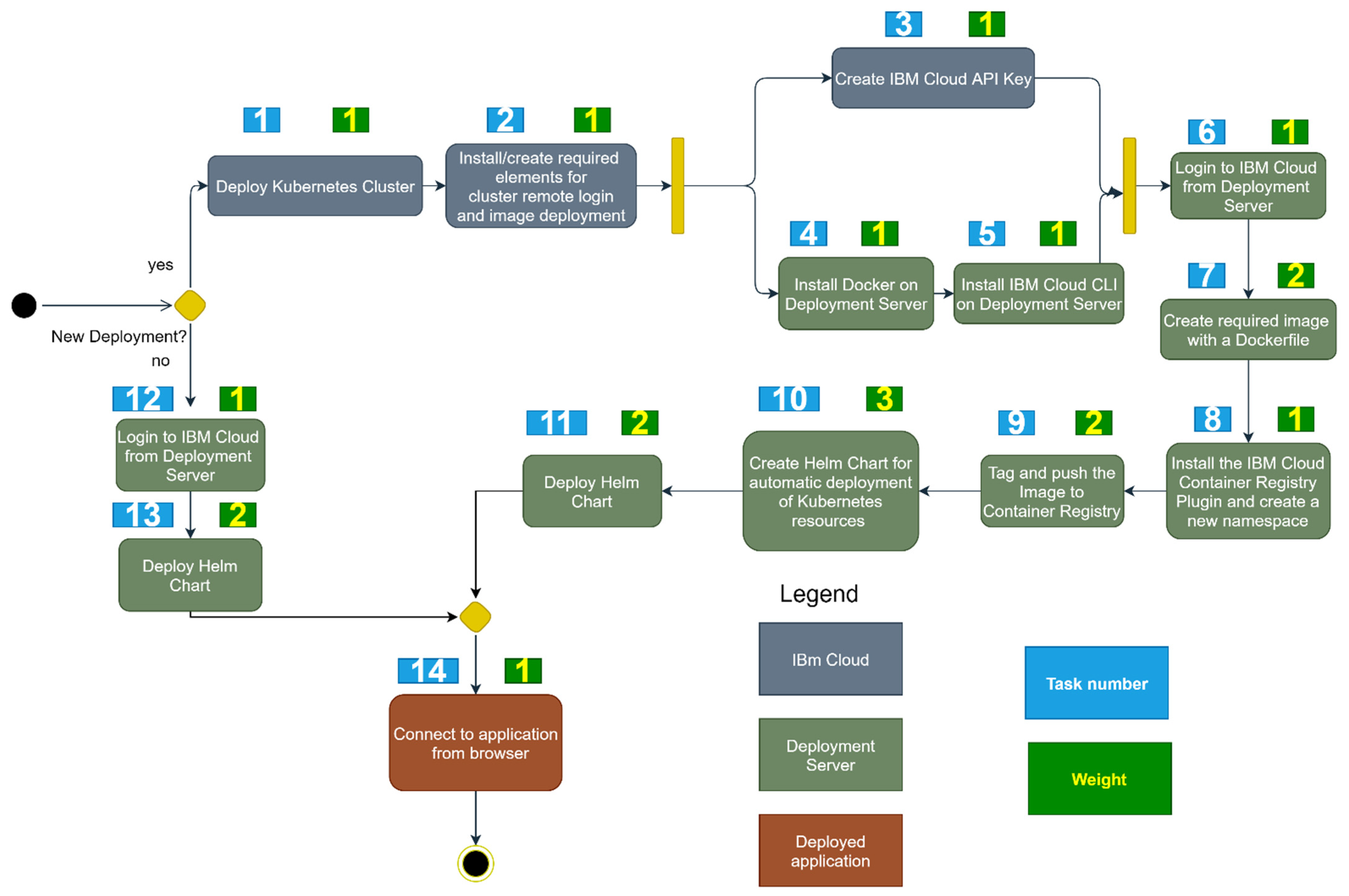
Let us first analyze the manual deployment process from Figure 1. For the tasks performed in IBM Cloud, marked with blue in Figure 1, a weight of 3 is assigned. For the deployment and preparation tasks, marked with green (prerequisites executed on a deployment server), a weight of 4 is given. For the last activity marked in red, the weight is 1. Start and End have 0 values. Therefore, $D_j$ represents the sum of the previously mentioned weighted tasks.

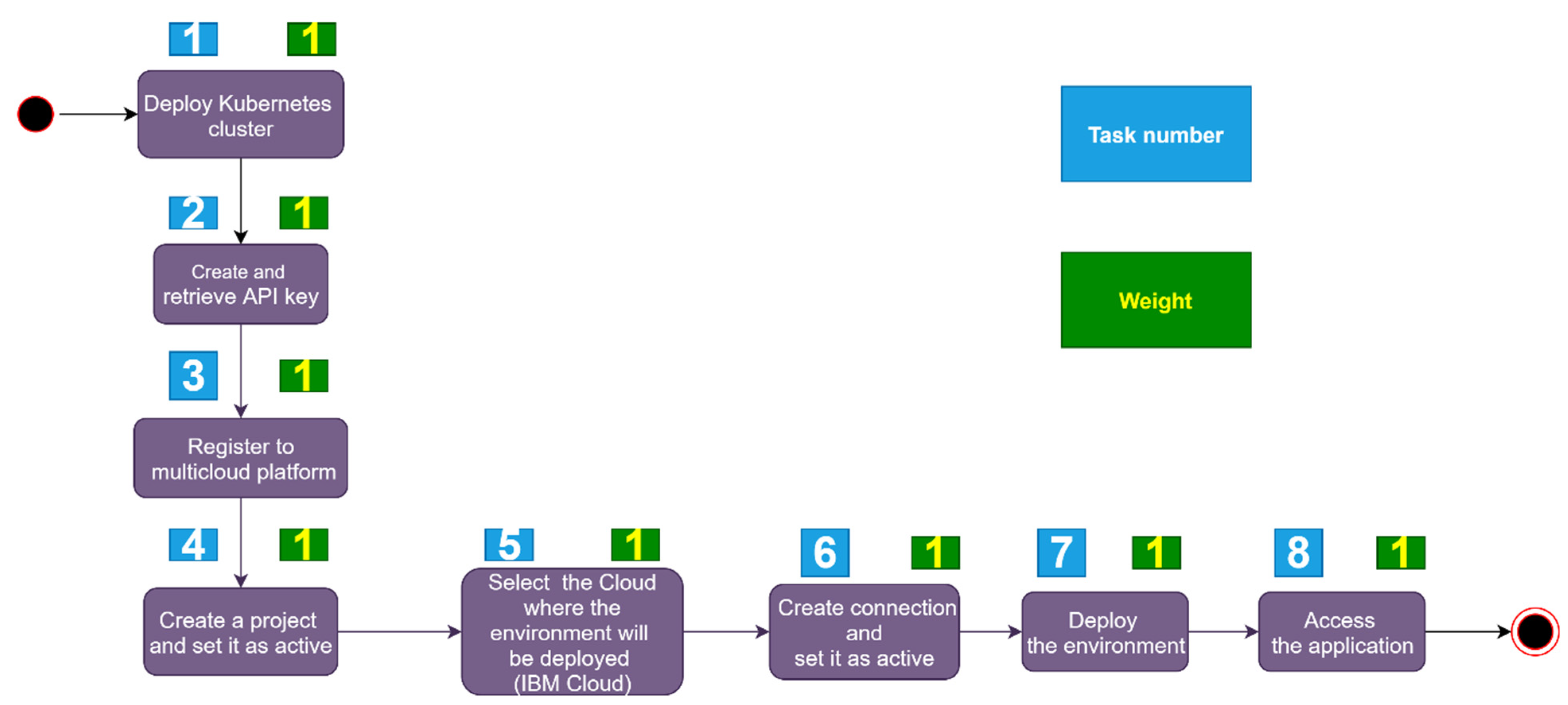
Then, let us analyze the automated process from Figure 2. For the first three tasks that require work on the cloud platform, a weight of 3 is assigned, and for the last five tasks that require work on the deployment platform, the weight is 1. Start and End weigh 0.

As a result, after applying the Equations (9) and (10) with the values presented above, $C_D$ has the value of 23.5 for the manual deployment process and 14 for the automated one.

After applying the equations from Section 3.2, the values of the parameters necessary for the computation of the Yaqin complexity are given in

Table 6. Parameter values for Yaqin complexity of the two deployment processes.

Parameter	Value for the Manual Deployment	Value for the Automated Deployment
Starts size (Ss)	1	1
Ends size (Es)	1	1
Intermediates size (Is)	0	0
Activities size (Acs)	20	10
Branching types (Bt)	2	0

. They were obtained by applying the equations to the processes for the manual deployment in Figure 1 and the automated deployment in Figure 2. After the individual calculation of the Yaqin equation components, the results are presented in

Table 7. Components of the Yaqin complexity for the two deployment processes.

Component	Value for the Manual Deployment	Value for the Automated Deployment
Number of nodes (Ns)	24	12
Arcs size (As)	21	9
Complexity of AND branch $(C_{\mathit{AND}}$)	6	0
Complexity of XOR branch $(C_{\mathit{XOR}}$)	0	0
Complexity of OR branch $(C_{\mathit{OR}})$	4	0
Cyclic complexity $(C_{\mathit{CYC}}$)	0	0
Depth complexity $(C_D$)	23.5	14

.

After calculating all the equations with the values resulting from Table 5, Table 6 and Table 7, the Yaqin complexity (YC) is 78.5 for manual deployment and 35 for automated deployment.

4.3. Complexity of Human Tasks

Let us now evaluate the complexity metric from Equation (11), introduced in Section 3.2. For this purpose, we assign specific weights to the manual and automated deployment processes, as illustrated in Figure 3 and Figure 4, respectively. The weights for each task and the motivation for their assignment are given in

Table 8. Weights for the manual deployment tasks.

Task Number	Weight (Wt)	Motivation
1	1	The deployment in the cloud of a Kubernetes cluster as a service is not difficult; the user needs to follow a simple procedure.
2	1	The installation of prerequisites is straightforward and requires minimum or no technical knowledge.
3	1	The API key is created after a few clicks on the cloud console.
4	1	The user needs to follow a simple procedure to install Docker on a Linux machine. On the new distribution of Linux (RHEL 8 and above), Podman is already installed and can be used in place of Docker.
5	1	The IBM Cloud CLI can be installed following a simple procedure.
6	1	Remote cloud login is straightforward and is done by running a command in the terminal.
7	2	For Docker Image creation, technical knowledge and understanding of the technology are required.
8	1	The IBM Cloud Container Registry plugin can be installed by following a procedure.
9	2	The tag and push notions are a little advanced for a normal user and require technical knowledge and technology understanding (Docker).
10	3	The creation of the Helm charts for automation and the deployment methods requires vast technical knowledge and some experience in working with technologies such as Kubernetes and Helm Charts.
11	2	Helm chart deployment requires technical knowledge.
12	1	Similar to task 6.
13	2	Similar to task 11.
14	1	Simple connection to the tool

for the manual deployment and in

Table 9. Weights for the automated deployment tasks.

Task Number	Weight (Wt)	Motivation
1	1	The deployment of Kubernetes cluster as a service is not hard in the cloud; the user needs to follow a simple procedure
2	1	The API key is created after a few clicks on the cloud console.
3	1	The deployment platform is a user-friendly environment
4	1	Project creation on the platform is very intuitive
5	1	This task is simple due to the ease of use of the platform
6	1	The deployment platform provides an intuitive menu for this task
7	1	The deployment is done by simply clicking a button
8	1	The tool is accessed from the browser

for the automated one.

Based on the weights assessed in Table 6 and Table 7, the resulting complexity of human tasks (CH)—calculated with the specific metric proposed in Section 3.2—is 20 for the manual deployment and 8 for the automated one.

4.4. Performance Test Results

Apart from the results obtained at the statical evaluation, this section presents the performance obtained in executing the tests with Prometheus and Grafana and Sysdig, for the deployment of WebGME—the software environment to be deployed, chosen for test purposes, as described previously in Section 3.4.

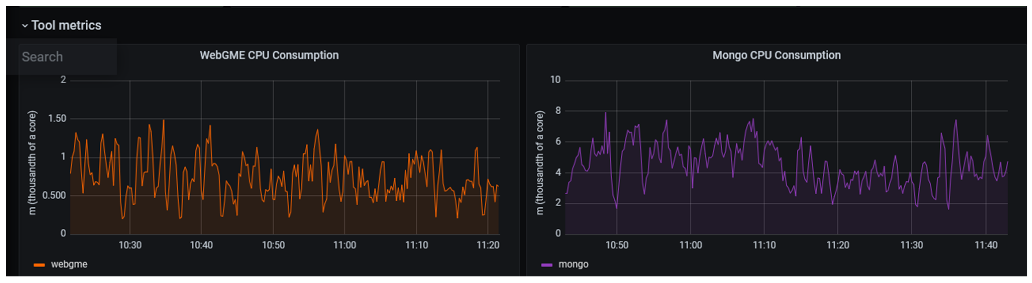
The results for the monitoring tool metrics are given in

Table 10. Prometheus monitoring results for containers.

Metric	Result (1 h Time Span)
Container CPU Mongo	2 m ÷ 8 m
Container Memory Mongo	70 MB
Container CPU Webgme	0.5 m ÷ 2 m
Container Memory Webgme	90 MB

. These metrics are used for performance measurement, and they also indicate the usage of the application. They were obtained by running the Prometheus PromQL queries presented in Table 2. The queries provide real-time data that help the user visualize the state of the deployed resources. These test results are obtained after the normal usage of the application by two users; the CPU resources are measured in thousands of cores—millicores (m). The Mongo and WebGME pods CPU consumptions are given in Figure 5.

The results of the cluster monitoring are presented in

Table 11. Prometheus cluster metrics results.

Metric	Result
Cluster memory usage	47.5%
Total memory	3.84 GB
Used memory	1.82 GB
Cluster CPU usage	21.34%
Total CPU	2 cores
Used CPU	0.43 cores

. They were obtained using the queries from Table 3. The purpose of these queries is to monitor the state of the cluster resources during the application execution The results represent the average consumption during a time span of one hour.

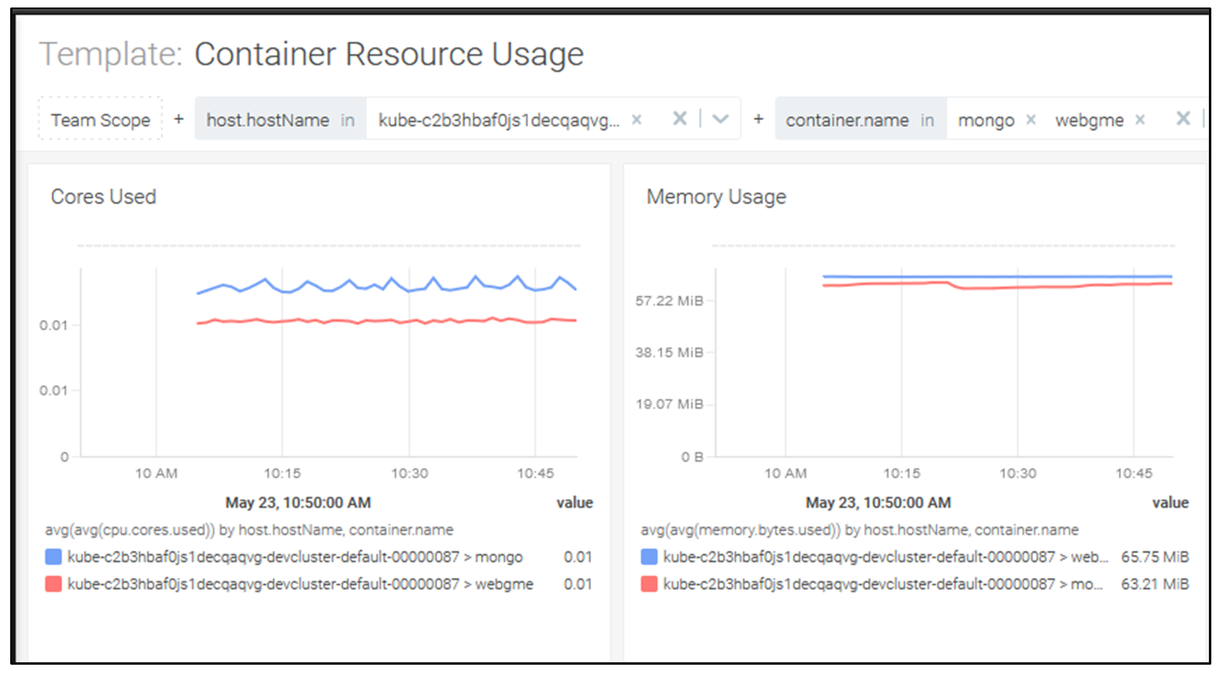
For the purpose of comparison,

Table 12. Sysdig monitoring results for containers.

Metric	Result (1 h Time Span)
Container CPU Mongo	0.01 cores
Container Memory Mongo	63.21 MB
Container CPU WebGME	0.01 cores
Container Memory WebGME	65.75 MB

also showcases the results of the metrics presented on the Sysdig console. They are obtained in the same conditions as the ones encountered during the Prometheus PromQL querying and represent the CPU and memory consumptions for the Mongo and WebGME containers; the CPU resources are measured in cores. The Sysdig monitoring dashboard in IBM Cloud provides real-time data regarding the CPU and memory for the mongo and webgme containers, during a period of 1 h (see Figure 6). On the left-hand side of the figure, there is information regarding CPU, measured in cores, and on the right-hand side regarding the memory, measured in mebibytes. On the left-hand side graph, the cores used for the webgme container are depicted in red and those for the mongo container in blue. On the right-hand side graph, the memory usage for the webgme container is represented in blue and for the mongo container in red. The average CPU and memory consumption monitored with this dashboard correspond to the values from Table 12.

Regarding the memory and CPU usage of the cluster, they are monitored in a default dashboard on the Sysdig console. As this is not a custom dashboard, we obtained the percentage of consumed CPU and memory presented in

Table 13. Sysdig cluster metrics results.

Metric	Result
Cluster memory usage (%)	30.74%
Cluster CPU usage (%)	23.63%

. The results represent the average consumption for one hour.

5. Discussion

We discuss the results obtained from the complexity analysis (Section 5.1) and the monitoring outputs of the performance testing (Section 5.2). Then, Section 5.3 presents the automated deployment platform whose development was motivated by the results obtained in this research.

5.1. Complexity Analysis

The results from Section 4.1 show that the cyclomatic complexity for automated deployment is 1, whereas that for manual deployment is 3. This was obtained after applying Equation (1) using the values from Table 4. As expected, the automated method has a lower cyclomatic complexity value than the manual one. The implication of this finding is important to our goal, as it is a first step to prove that the development of an automated deployment platform would make a significant difference. A lower complexity value indicates fewer errors, a process that is easier to understand by the user, easier to test, and easier to maintain.

For the two deployment processes (represented in Figure 1 and Figure 2) the Yaqin complexity (YC) results presented in Section 4.2 also differ. First, we notice that the first process, for the manual deployment, is more complex than the automated deployment due to the difference in the number of branches. However, this is not the only reason; this is one of the strengths of the method proposed in [7], because the Yaqin metric involves many parameters and it is very sensitive in finding the differences between the branches’ numbers and types (OR, AND, and XOR). These results presented in detail in Table 5, Table 6 and Table 7 led us to observe that the overall Yaqin complexity is more than double for the manual deployment process than for the automated one. This result confirms the advantage of a deployment platform and its simplicity of use in comparison with the manual method.

As a supplementary evaluation, let us also consider the complexity of the human tasks (CH) estimated in Section 4.3. This is more specific to the scope of our research and the assignment of the weights is motivated in Table 8 and Table 9. The assigned weights are between 1 and 3, with the value 3 for the most complex tasks. In the case of automated deployment, not a single task was given a weight of 3, in contrast with manual deployment. According to this metric, CH is 20 for the manual deployment, and only 8 for the automated one, i.e., almost seven times lower. This is a significant difference, though a deployment platform allows an important reduction of manual work, also enlarging the range of people who are able to deploy the software environment they need to the cloud, without the need for highly specialized technical knowledge in cloud computing. Note that the CH metric defined in Section 4.3 is similar to the YC metric, because it also employs cognitive weight to evaluate the difficulty of understanding the software. With the specific metric, we customize this method to the tasks needed to prepare/deploy/use an environment. The chosen criteria may be also applied to other similar processes, which require various kinds of interaction with the user to perform manual tasks.

For the deployment on other cloud platforms, the steps presented in Figure 3 and Figure 4 are similar, with several differences regarding the cloud provider-specific offerings. For example, for the manual deployment, task 3 in Figure 3 should implement specific Azure or AWS connection methods, such as service principal ID and password, or AWS access key ID and secret access key. Task 5 would be replaced with the installation of the respective cloud CLI and task 6 would connect to the chosen cloud platform. For task 8, there are several alternatives up to the preferences of the user. For example, one can use AWS Elastic container registry, Azure container registry, or Docker Hub. Of course, task 12 would also change to require the connection to the targeted cloud platform. For the automated deployment process, task 2 in Figure 4 would require the user to retrieve the specific AWS and Azure credentials; task 5 becomes the selection of the targeted cloud, and task 6 would create the connection to the selected cloud from the multicloud platform. Therefore, the steps are slightly different to suit the cloud provider-specific and do not need to be changed entirely. The complexity value remains the same for deployment in other cloud platforms. The specific provisioning models on these cloud platforms do not make a noticeable difference in the deployment of the software environment, because they all use a Kubernetes service and the deployment is realized with the same methods, i.e., Helm Charts.

5.2. Performance Analysis

For performance testing, we used Prometheus (version 2.25.0) and Sysdig for monitoring the Kubernetes cluster and the deployed containers. The performance of the software environment installed on a container, in a pod, is evaluated through the Kube-state metrics, and Prometheus is configured to scrape these metrics. The metrics characterize the state of the resources that reside on a Kubernetes cluster, such as pod deployments. For Sysdig, an agent is installed automatically on the Kubernetes cluster when the service is enabled in the cloud provider console. This agent has the role to deliver metrics for the Kubernetes resources that reside on the cluster, and it is installed on every node because it is deployed as a daemonset. The container CPU and memory metrics indicate the usage of an application and its efficiency. If an application is inefficient and the memory increases at an alarming level for the cluster, an ut of Memory (OOM) signal may appear on the respective worker logs; in such a case, the pod that consumes too much memory is evicted and rescheduled. If the graph shows alarming memory and CPU consumptions, the memory limits must become higher than the memory request, but not as high as the entire worker memory. The CPU and memory consumption PromQL queries were described in Table 2. These queries are made on Prometheus to obtain results in Grafana (which uses Prometheus as a data source). For Sysdig, a monitoring agent is installed on the cluster when this service is enabled in IBM Cloud. In this case, the metrics for CPU and memory consumption of a container are part of the standard offering of the tool.

After calculating these metrics for our testing environment (see Table 10) and based on the cluster memory and CPU usage from Table 11 and Table 13, we consider that the current sizing is capable of sustaining the WebGME modeling environment alongside the monitoring solution. The memory consumption of the Kubernetes pods can be controlled by introducing memory requests and limits to the container definition inside a deployment. Those configuration parameters have the role of preventing the container to use more resources than it is intended. When the limit is reached, the container is restarted [37]. However, the strain may increase if many users actively utilize the same service, i.e., access the modeling environment as a service at the same time. In comparison to these findings, obtained with Prometheus and Grafana, the Sysdig results from Table 12 are relatively similar. Both tests return results below 100 MB for the consumed memory, for both WebGME and Mongo. Due to the limitations of resources on the Kubernetes cluster used in our testing environment, this cannot be tested at the same time. The difference in the case of CPU is because the measuring unit used in both tests is different. In the Sysdig monitoring dashboard, cores are used as CPU monitoring units, whereas on Grafana the thousandth of a core (m) has been chosen. Hence, the approach used in Grafana is more sensitive to lower CPU consumption in comparison with the core approximation used on the Sysdig dashboard.

The results from Table 11 and Table 13 prove a lower memory consumption when Prometheus and Grafana are not installed on the cluster, although the CPU consumption is similar. This may be considered an advantage of the Sysdig IBM Cloud monitoring, alongside the fact that it requires no configuration from the user side. The disadvantage is that Sysdig is not present in this form in other cloud platforms, such as Azure and AWS.

For more than two users, the CPU and memory consumption can grow depending on the number of users who use the environment concomitantly. From the Kubernetes perspective, this consumption can be limited to what a cluster has in terms of resources, by configuring memory and CPU limits for the pod that contains the software environment. If the memory limit is reached, the pod is restarted automatically to maintain the resource consumption between the expected thresholds. Furthermore, a real-life test is needed with multiple users, as well as a method to predict how many resources are needed with respect to the users. This is a topic for future work, resulting in a feature added to the deployment platform to advise the users regarding the sizing of the cluster, in relationship with the maximum number of users that are expected.

5.3. Automated Deployment Platform

The research presented in this paper showed that an automated deployment would make an important difference in the accessibility of a software environment delivered as a service in the cloud. The resulting platform for automated cloud deployment is written in Node.js for the backend part, and in Angular for the frontend. The platform is designed to deploy multiple kinds of software environments to cloud environments having different providers, with the possibility to add new ones to the list.

The platform is capable of automating the deployment of the WebGME modeling and metamodeling environment in IBM Cloud, AWS, and Azure. Early work was presented in [38,39]. Currently, the deployment is realized using technologies such as Docker, Kubernetes, and Helm; they were chosen because they also work well with other important cloud providers, not only with IBM Cloud. To start the deployment, a user is required to register to the platform, create a project, set it as active, and register the cloud connection credentials in the form required for the chosen cloud provider. As future work, the platform will also support the deployment of the Kubernetes service; depending on the chosen cloud provider, the user will have a tutorial on how to deploy a Kubernetes service on the cloud platform.

Thus, the platform for automated software environment deployment in the cloud provides non-technical users with the opportunity of an easier setup and a fast deployment of the needed software environment in the cloud. It is also possible to create multiple environments for test, development, and production whenever needed. The deployed software environment can also be automatically deleted by the user through the platform. In future work, the platform will support the automatic deployment of other software environments and the deployment of the Kubernetes service on IBM Cloud, Azure, and AWS.

6. Conclusions

From the point of view of the users, a high level of complexity may be a decisive factor in choosing a cloud solution. Difficulties can arise if it is too hard to make a deployment of the software environment due to limited skills in cloud computing technologies. Nonetheless, a complex environment with extensive resources may be needed for the deployed software to be able to run smoothly. These are current challenges for someone who is planning a solution and has to find out if the environment is fit enough from the sizing perspective. They are overcome by analyzing how to make the manual tasks of deployment less complex and determining how the deployed resources behave in real-life scenarios.

This study evaluated the manual and automated processes for deploying a software environment into the cloud, adopting a container-based solution. The aim was to determine whether the difference in their complexity is significant enough to influence the decision to make the deployment into the cloud and adopt an Environment as a Service approach. The two processes were modeled and analyzed statically, using three types of metrics: the classical cyclomatic complexity, the more advanced assembly of metrics for Yaqin complexity, and a specific metric proposed in this paper for the complexity of human tasks required for deployment. The weight assignment criteria used in this specific metric are based on the amount of knowledge needed by a user/developer to complete a task. The analysis proved that the cyclomatic complexity is three times smaller for automated than for manual deployment. The Yaqin complexity is more than two times lower, and the complexity of human tasks is seven times lower. Apart from the static analysis, the study included the performance monitoring realized with Prometheus and Grafana and then with Sysdig, with a Kubernetes service provided by IBM Cloud and WebGME as an example of a software environment. The results on process complexity and performance proved the opportunity of using a platform for the automated deployment of a software environment. The extension to multicloud is also possible, by adapting several process activities.

References

- Tomarchio, O.; Calcaterra, D.; Di Modica, G. Cloud resource orchestration in the multi-cloud landscape: A systematic review of existing frameworks. J. Cloud Comput. Adv. Syst. Appl. 2020, 9, 1–24. [Google Scholar] [CrossRef]
- Giannakopoulos, I.; Konstantinou, I.; Tsoumakos, D.; Koziris, N. Cloud application deployment with transient failure recovery. J. Cloud Comput. Adv. Syst. Appl. 2018, 7, 11. [Google Scholar] [CrossRef]
- Li, G.; Woo, J.; Lim, S.B. HPC Cloud Architecture to Reduce HPC Workflow Complexity in Containerized Environments. Appl. Sci. 2021, 11, 923. [Google Scholar] [CrossRef]
- Shah, S.A.R.; Waqas, A.; Kim, M.-H.; Kim, T.-H.; Yoon, H.; Noh, S.-Y. Benchmarking and Performance Evaluations on Various Configurations of Virtual Machine and Containers for Cloud-Based Scientific Workloads. Appl. Sci. 2021, 11, 993. [Google Scholar] [CrossRef]
- Bystrov, O.; Pacevič, R.; Kačeniauskas, A. Performance of Communication- and Computation-Intensive SaaS on the OpenStack Cloud. Appl. Sci. 2021, 11, 7379. [Google Scholar] [CrossRef]
- Shepperd, M. A critique of cyclomatic complexity as a software metric. Softw. Eng. J. 1988, 3, 30–36. [Google Scholar] [CrossRef]
- Yaqin, M.; Sarno, R.; Rochimah, S.; Nopember, I.T.S. Measuring Scalable Business Process Model Complexity Based on Basic Control Structure. Int. J. Intell. Eng. Syst. 2020, 13, 52–65. [Google Scholar] [CrossRef]
- Ferrer, A.J.; Pérez, D.G.; González, R.S. Multi-cloud Platform-as-a-service Model, Functionalities and Approaches. Procedia Comput. Sci. 2016, 97, 63–72. [Google Scholar] [CrossRef] [Green Version]
- Rani, B.K.; Babu, A.V. Cloud Computing and Inter-Clouds—Types, Topologies and Research Issues. Procedia Comput. Sci. 2015, 50, 24–29. [Google Scholar] [CrossRef] [Green Version]
- Ritter, D. Cost-aware process modeling in multiclouds. Inf. Syst. 2021, 101969. [Google Scholar] [CrossRef]
- Velde, V.; Mandala, S.K.; Vurukonda, N.; Ramesh, D. Enterprise based data deployment inference methods in cloud infrastructure. Mater. Today Proc. 2021. [Google Scholar] [CrossRef]
- Wang, L.-C.; Chen, C.-C.; Liu, J.-L.; Chu, P.-C. Framework and deployment of a cloud-based advanced planning and scheduling system. Robot. Comput. Manuf. 2020, 70, 102088. [Google Scholar] [CrossRef]
- Revuri, V.; Ambika, B.; Kumar, D.S.; Reddy, C.L. High performance research implementations with third party cloud platforms and services. Mater. Today Proc. 2021. [Google Scholar] [CrossRef]
- Afgan, E.; Lonie, A.; Taylor, J.; Goonasekera, N. CloudLaunch: Discover and deploy cloud applications. Future Gener. Comput. Syst. 2018, 94, 802–810. [Google Scholar] [CrossRef] [PubMed] [Green Version]
- De Gouw, S.; Mauro, J.; Zavattaro, G. On the modeling of optimal and automatized cloud application deployment. J. Log. Algebraic Methods Program. 2019, 107, 108–135. [Google Scholar] [CrossRef] [Green Version]
- Kovács, J.; Kacsuk, P.; Emődi, M. Deploying Docker Swarm cluster on hybrid clouds using Occopus. Adv. Eng. Softw. 2018, 125, 136–145. [Google Scholar] [CrossRef]
- Sukesh, M.; Kumar, R.N.; Reddy, C.L. Development and deployment of real-time cloud applications on red hat OpenShift and IBM bluemix. Mater. Today Proc. 2021. [Google Scholar] [CrossRef]
- Muketha, G.; Ghani, A.; Selamat, M.; Atan, R. A Survey of Business Process Complexity Metrics. Inf. Technol. J. 2010, 9, 1336–1344. [Google Scholar] [CrossRef] [Green Version]
- Ikerionwu, C. Cyclomatic complexity as a Software metric. Int. J. Acad. Res. 2010, 2. Available online: https://www.researchgate.net/publication/264881926_Cyclomatic_complexity_as_a_Software_metric (accessed on 21 February 2022).
- Dijkman, R.; Dumas, M.; van Dongen, B.; Käärik, R.; Mendling, J. Similarity of business process models: Metrics and evaluation. Inf. Syst. 2011, 36, 498–516. [Google Scholar] [CrossRef] [Green Version]
- Cardoso, J.; Mendling, J.; Neumann, G.; Reijers, H.A. A Discourse on Complexity of Process Models. In Proceedings of the International Conference on Business Process Management, Vienna, Austria, 5–7 September 2006; pp. 117–128. [Google Scholar] [CrossRef]
- Muketha, G.; Ghani, A.; Selamat, M.; Atan, R. Complexity Metrics for Executable Business Processes. Inf. Technol. J. 2010, 9, 1317–1326. [Google Scholar] [CrossRef] [Green Version]
- Jao, S.; Yang, Y. A new measure of software complexity based on cognitive weight. Can. J. Electr. Comput. Eng. 2003, 28, 69–74. [Google Scholar] [CrossRef]
- Gruhn, V.; Laue, R. Adopting the Cognitive Complexity Measure for Business Process Models. In Proceedings of the 5th IEEE International Conference on Cognitive Informatics, Beijing, China, 17–19 July 2006; pp. 236–241. [Google Scholar] [CrossRef]
- Aslanpour, M.S.; Gill, S.S.; Toosi, A.N. Performance evaluation metrics for cloud, fog and edge computing: A review, taxonomy, benchmarks and standards for future research. Internet Things 2020, 12, 100273. [Google Scholar] [CrossRef]
- Al-Faifi, A.M.; Song, B.; Hassan, M.M.; Alamri, A.; Gumaei, A. Data on performance prediction for cloud service selection. Data Brief 2018, 20, 1039–1043. [Google Scholar] [CrossRef] [PubMed]
- Krebs, R.; Momm, C.; Kounev, S. Metrics and techniques for quantifying performance isolation in cloud environments. Sci. Comput. Program. 2014, 90, 116–134. [Google Scholar] [CrossRef]
- Ahmad, A.A.-S.; Andras, P. Scalability analysis comparisons of cloud-based software services. J. Cloud Comput. Adv. Syst. Appl. 2019, 8, 1–17. [Google Scholar] [CrossRef]
- Prometheus Overview. Available online: https://prometheus.io/docs/introduction/overview/ (accessed on 5 April 2021).
- Sysdig Monitor. Available online: https://docs.sysdig.com/en/sysdig-monitor.html (accessed on 20 May 2021).
- Prometheus Configuration Kubernetes. Available online: https://devopscube.com/setup-prometheus-monitoring-on-kubernetes/ (accessed on 1 May 2021).
- Kube State Metrics Configuration. Available online: https://devopscube.com/setup-kube-state-metrics/ (accessed on 1 May 2021).
- Grafana Setup. Available online: https://devopscube.com/setup-grafana-kubernetes/ (accessed on 1 May 2021).
- GME: Generic Modeling Environment. Available online: http://www.isis.vanderbilt.edu/projects/GME (accessed on 5 April 2021).
- Maróti, M.; Kecskes, T.; Kereskényi, R.; Broll, B.; Völgyesi, P.; Jurácz, L.; Levendoszky, T.; Ledeczi, A. Next generation (Meta)modeling: Web- and cloud-based collaborative tool infrastructure. CEUR Workshop Proc. 2014, 1237, 41–60. [Google Scholar]
- Maróti, M.; Kereskényi, R.; Kecskés, T.; Völgyesi, P.; Lédeczi, A. Online Collaborative Environment for Designing Complex Computational Systems. Procedia Comput. Sci. 2014, 29, 2432–2441. [Google Scholar] [CrossRef] [Green Version]
- Kubernetes Requests and Limits. Available online: https://kubernetes.io/docs/concepts/configuration/manage-resources-containers/ (accessed on 16 August 2021).
- Anton, F.D.; Ionita, A.D. Cloud-Enabled Modeling of Sensor Networks in Educational Settings. In Big Data Platforms and Applications. Computer Communications and Networks; Pop, F., Neagu, G., Eds.; Springer International Publishing: Berlin/Heidelberg, Germany, 2021. [Google Scholar] [CrossRef]
- Lacatusu, M.; Lacatusu, F.; Damian, I.; Ionita, A.D. Multicloud deployment to support remote learning. In Proceedings of the International Technology, Education and Development Conference, Orlando, FL, USA, 8–9 March 2021; pp. 4601–4606. [Google Scholar] [CrossRef]
Figure 1.
The manual deployment process for the IBM Cloud.
Figure 2.
The automated deployment process for the IBM Cloud.
Figure 3.
The weighted manual deployment process.
Figure 4.
The weighted automated deployment process.
Figure 5.
Mongo and WebGME pods CPU consumptions.
Figure 6.
Sysdig monitoring dashboard.