Exploring Early Prediction of Chronic Kidney Disease Using Machine Learning Algorithms for Small and Imbalanced Datasets

Abstract

Chronic kidney disease (CKD) is a worldwide public health problem, usually diagnosed in the late stages of the disease. To alleviate such issue, investment in early prediction is necessary. The purpose of this study is to assist the early prediction of CKD, addressing problems related to imbalanced and limited-size datasets. We used data from medical records of Brazilians with or without a diagnosis of CKD, containing the following attributes: hypertension, diabetes mellitus, creatinine, urea, albuminuria, age, gender, and glomerular filtration rate. We present an oversampling approach based on manual and automated augmentation. We experimented with the synthetic minority oversampling technique (SMOTE), Borderline-SMOTE, and Borderline-SMOTE SVM. We implemented models based on the algorithms: decision tree (DT), random forest, and multi-class AdaBoosted DTs. We also applied the overall local accuracy and local class accuracy methods for dynamic classifier selection; and the k-nearest oracles-union, k-nearest oracles-eliminate, and META-DES for dynamic ensemble selection. We analyzed the models’ performances using the hold-out validation, multiple stratified cross-validation (CV), and nested CV. The DT model presented the highest accuracy score (98.99%) using the manual augmentation and SMOTE. Our approach can assist in designing systems for the early prediction of CKD using imbalanced and limited-size datasets.

1. Introduction

The high prevalence and mortality rates of persons with chronic diseases, such as chronic kidney disease (CKD) [1], are real-world public health problems. The world health organization (WHO) estimated that chronic diseases would cause 60 percent of the deaths reported in 2005, 80 percent in low-income and lower-middle-income countries, increasing to 66.7 percent in 2020 [2]. According to the WHO health statistics 2019 [3], people who live in low-income and lower-middle-income countries have a higher probability of dying prematurely from known chronic diseases such as diabetes mellitus (DM). Estimates reveal that in 2045, about 628.6 million people will have DM, with 79% of them living in low-income and lower-middle-income countries [4].

For CKD’s specific case, the early prediction and monitoring of this disease and its risk factors reduce the CKD progression and prevent adverse events, such as sudden development of diabetic nephropathy. Thus, this study considers CKD early prediction and monitoring focusing on a dataset from people who live in Brazil, a continental-size developing country. Developing countries stand for low- and middle-income regions, while developed countries are high-income regions, such as the USA [5]. Developing countries suffer from increased mortality rates caused by chronic diseases, e.g., CKD, arterial hypertension (AH), and DM [6]. AH and DM are two of the most common CKD risk factors. People with type 1 or type 2 DM are at high risk of developing diabetic nephropathy [7], while severe AH cases may increase kidney damage. For example, in 2019, about 10 percent of the adult Brazilian population was aware of having kidney damage, while about 70 percent remained undiagnosed [8].

The CKD is characterized by permanent damage, reducing the kidneys’ excretory function, measured using glomerular filtration [9]. However, the diagnosis usually occurs during more advanced stages because it is asymptomatic, postponing the application of countermeasures, decreasing people’s quality of life, and possibly leading to lethal kidney damage. For example, in 2010, about 500–650 people per million of the Brazilian population faced dialysis and kidney transplantation [10]. This number has grown, warning governments about the relevance of the CKD early prediction. In 2016, according to the Brazilian chronic dialysis survey, the number of patients under dialysis was 122,825.00, increasing this number by 31,000.00 in the last five years [11]. In 2017, the prevalence and incidence rates of patients under dialysis were 610 and 194 per million [12]. The incidence continued to be high in 2018 (133,464.00) [13]. Estimates also indicate that, in 2030, about 4 million patients will be under dialysis worldwide [14].

The high prevalence and incidence of dialysis and kidney transplantation increase public health costs. Therefore, CKD has an expressive impact on the health economics perspective [15]. For instance, the Brazilian Ministry of Health reported that transplantation and its procedures spent about 720 million reais in 2008 and 1.3 billion in 2015 [16]. According to the Brazilian Ministry of Health, in 2020, the Brazilian government spent more than 1.4 billion reais for hemodialysis procedures. The costs and the high rates of persons waiting for transplantation suggest the increased public spending on kidney diseases. Preventing CKD has a relevant role in reducing mortality rates and public health costs [17]. The CKD early prediction is even more challenging for people who live in remote and hard-to-reach settings because of either lack of or precarious primary care. CKD early prediction is relevant to improve CKD screening and reduce public health costs.

In this study, we address four problems. The first problem is size limitation, in which training models using small datasets can result in skewed performance estimates [18]. The second problem is the imbalance problem [19], in which models may underperform in minority classes, producing misleading results [20]. The third problem is the choice of the algorithm to address imbalanced and limited-size datasets. The fourth problem is the early prediction of CKD using risk levels (low risk, moderate risk, high risk, and very high risk) and a reduced number of biomarkers. CKD datasets with risk level evaluation are very scarce and of limited size. The majority of available datasets are composed of binary classes. The analyses based on risk levels enable patients to have more detailed explanations about the evaluation results. In the medical area, the availability of imbalanced and limited-size datasets is common. Although the usage of limited-size datasets may be questioned, it is already evidenced that such datasets can be relevant for the medical area [21].

Our study relies on data from medical records of Brazilians to provide classification models to assist in the early prediction of CKD in developing countries. We performed comparisons between machine learning (ML) models, considering ensemble and non-ensemble approaches. This work complements the results presented in our previous study [5], where a comparative analysis was performed with the following ML techniques: decision tree (DT), random forest (RF), naive Bayes, support vector machine (SVM), multilayer perceptron, and k-nearest neighbor (KNN). In such a previous study, DT and RF presented the highest performances. However, in our previous experiments, we did not apply automated oversampling techniques.

Notwithstanding, in the current study, we used the same Brazilian CKD dataset to enable the implementation and validation of the models: DT, RF, and multi-class AdaBoosted DTs. We conduct further experiments to improve the state-of-the-art by presenting an approach based on oversampling techniques. We applied the overall local accuracy (OLA) and local class accuracy (LCA) methods for dynamic classifier selection (DCS). We used the k-nearest oracles-union (KNORA-U), k-nearest oracles- eliminate (KNORA-E), and META-DES methods for dynamic ensemble selection (DES). We used such methods due to their usual high performance with imbalanced and limited size datasets [22]. The definitions of frequently used acronyms are presented in

Table 1. Summary of main acronyms.

Acronyms	Definition
CKD	Chronic Kidney Disease
WHO	World Health Organization
DM	Diabetes Mellitus
AH	Arterial Hypertension
ML	Machine Learning
DT	Decision Tree
RF	Random Forest
SVM	Support Vector Machine
KNN	K-Nearest Neighbor
OLA	Overall Local Accuracy
LCA	Local Class Accuracy
DCS	Dynamic Classifier Selection
KNORA-U	K-Nearest Oracles-Union
KNORA-E	K-Nearest Oracles-Eliminate
DES	Dynamic Ensemble Selection
SMOTE	Synthetic Minority Oversampling Technique
ROC	Receiver Operating Characteristic
PRC	Precision-Recall Curve
MCC	Matthew’s Correlation Coefficient
FMI	Fowlkes-Mallows
GFR	Glomerular Filtration Rate
ANN	Artificial Neural Network
OCT	Optical Coherence Tomography
PR	Precision
ACC	Accuracy score
PHR	Personal Health Records
DSS	Decision Support System
CDA	Clinical Document Architecture
GUI	Graphical User Interface
CV	Cross-Validation

.

For the implemented ensemble models, we prioritized the attributes of the dataset by applying the multi-class feature selection framework proposed by Pineda-Bautista et al. [23], including class binarization and balancing with the synthetic minority oversampling technique (SMOTE), evaluated with the receiver operating characteristic (ROC) curve and precision-recall curve (PRC) areas.

To address problems related to imbalanced and limited-size datasets, it is relevant to carry out data oversampling by rebalancing the classes before training the ML models [24,25]. We conducted experiments by oversampling the data from the medical records of Brazilian patients and comparing methods for resampling the data. We also used dynamic selection methods for further addressing such problems.

Besides, to deploy our approach, we developed a decision support system (DSS) to embed the ML model with the highest performance. In this article, the development of a DSS was relevant to discuss a clinical practice context, showing how our approach can be reused in a real-world scenario.

This work provides insights for developers of medical systems to assist in the early prediction of CKD to reduce the impacts of the late diagnosis, mainly in low-income and hard-to-reach locations, when using imbalanced and limited-size datasets. The main contributions of this work are: (1) the presentation of an approach for data oversampling (i.e., a combination of manual augmentation with automated augmentation); (2) the comparison of data oversampling techniques; (3) the comparison of validation methods; and (4) the comparison of ML models to assist the CKD early prediction in developing countries using imbalanced and limited size datasets. Therefore, one of the main technical novelties of this article relates to the presentation and evaluation of our oversampling approach that combines manual augmentation and automated augmentation.

2. Preliminaries

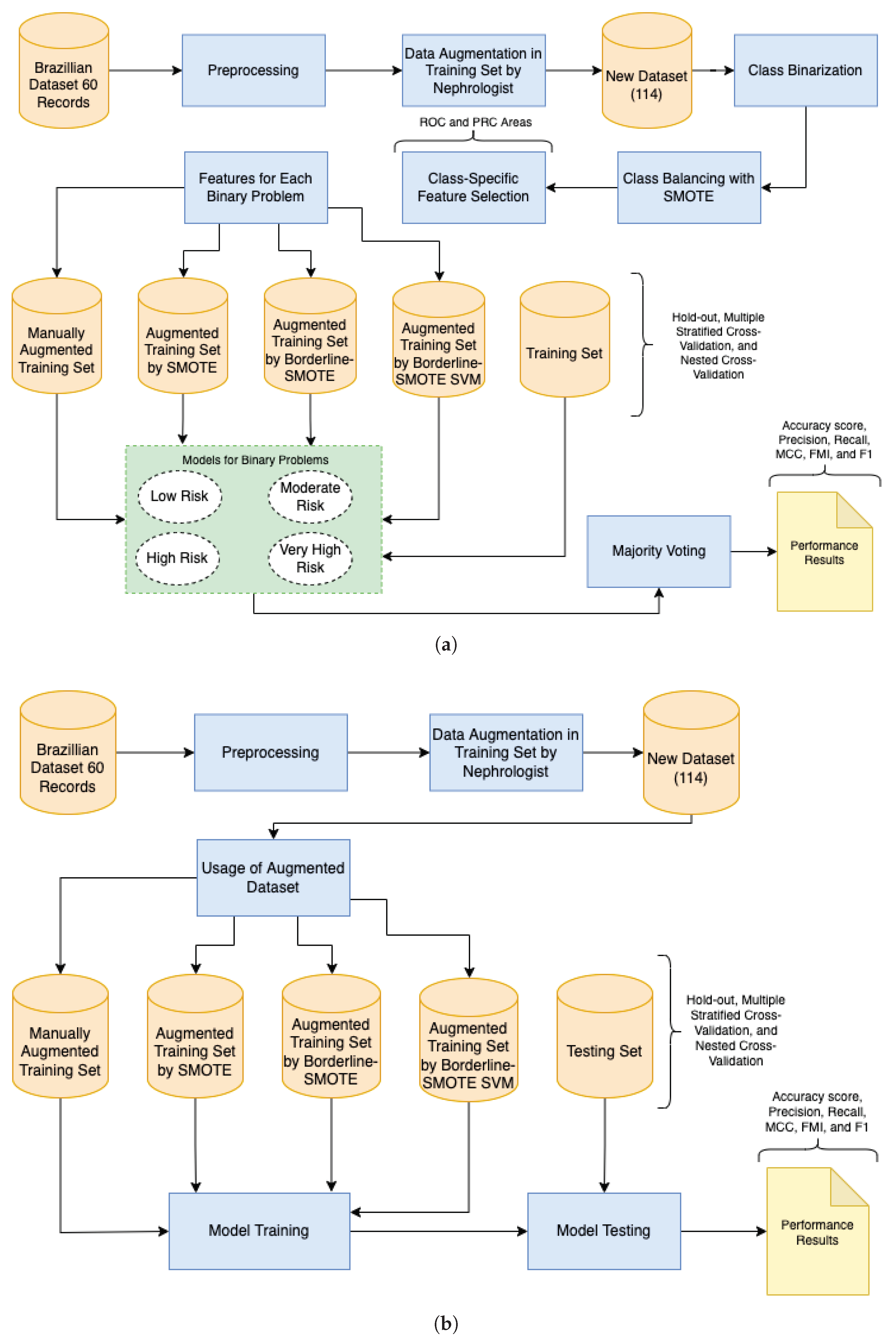
The research methodology of this study consists of data preprocessing, model implementation, validation methods, data augmentation, and multi-class classification metrics (Figure 1). Firstly, we preprocessed the Brazilian CKD dataset (i.e., binarization of attributes) and translated it to English.

We implemented ensemble (Figure 1a) and non-ensemble (Figure 1b) models using the algorithms DT, RF, and multi-class AdaBoosted DTs. We also selected the DCS (OLA and LCA) and DES (KNORA-U, KNORA-E, and META-DES) methods. We used the default configuration with a pool of classifiers of 10 decision trees. We chose this configuration because decision tree-based algorithms usually present high performance in imbalanced datasets. We implemented the ensemble models based on the framework proposed by Pineda-Bautista et al. [23].

We applied three ensemble and non-ensemble models validation methods: hold-out validation, multiple stratified CV, and nested CV. We used these methods to investigate whether they satisfactorily control overfitting caused due to the limited size of our dataset [26]. We applied the multiple stratified CV and nested CV with 10 folds and five repetitions. For the hold-out method, we split our dataset into 70% for training and 30% for testing. Thus, we conducted data augmentation only for the training set to ensure that the test set contained only real data. Our approach combines the data oversampling using: (1) manual augmentation, validated by an experienced nephrologist, and (2) automated augmentation (experimenting with the SMOTE, Borderline-SMOTE, and Borderline-SMOTE SVM).

Hence, we applied the following multi-class classification metrics: precision, accuracy score, recall, weighted F-score (F1), macro F1, Matthew’s correlation coefficient (MCC), Fowlkes-Mallows (FMI), ROC, and PRC. We used the python scikit-learn library [27] to implement the models and to apply the validation methods and metrics. For dynamic selection techniques, we used the DESlib library [22].

Figure 1. (a) Research steps based on the framework proposed by Pineda-Bautista et al. [23]: data preprocessing, model implementation, validation methods, data augmentation, and multi-class classification metrics. (b) Research steps based on simple approach: data preprocessing, model implementation, validation methods, data augmentation, and multi-class classification metrics.

Figure 1. (a) Research steps based on the framework proposed by Pineda-Bautista et al. [23]: data preprocessing, model implementation, validation methods, data augmentation, and multi-class classification metrics. (b) Research steps based on simple approach: data preprocessing, model implementation, validation methods, data augmentation, and multi-class classification metrics.

2.1. Data Collection and Preprocessing

In a previous study [28], we collected medical data (60 real-world medical records) from physical medical records of adult subjects (age ≥ 18) under the treatment of University Hospital Prof. Alberto Antunes of the UFAL, Brazil. The data collection from medical records maintained in a non-electronic format at the hospital was approved by the Brazilian ethics committee of UFAL and conducted between 2015 and 2016. The dataset comprises 16 subjects with no kidney damage, 14 subjects diagnosed only with CKD, and 30 subjects diagnosed with CKD, AH, and/or DM. In general, the sample included subjects with ages between 18 and 79 years; approximately 94.5% of the subjects were diagnosed with AH, and 58.82% were diagnosed with DM (

Table 2. Demographic, laboratory tests, and commodities of patients from the 60 real-world medical records.

Features	Patients
Gender (%)	F(41) M (19)
Age	Between 18 and 79 years
Creatinine, n (%)	60 (100%)
Urea, n (%)	60 (100%)
Albuminuria, n (%)	60 (100%)
Albuminuria, n (%)	60 (100%)
GFR, n (%)	60 (100%)
DM	Yes (15) No (45)
AH	Yes (29) No (31)

). With over 30 years of experience in CKD treatment and diagnosis in Brazil, a nephrologist labeled the risk classifications based on the KDIGO guideline [29]. The dataset with 60 medical records from the real world was classified into four risk classes: low risk (30 records), moderate risk (11 records), high risk (16 records), and very high risk (3 records).

We primarily selected dataset features based on medical guidelines. Specifically, the KDIGO guideline [29], the national institute for health and care excellence guideline [30], and the KDOQI guideline [31]. Besides, we interviewed a set of Brazilian nephrologists to confirm the relevance of the features in Brazil’s context. The final set of CKD features focusing on Brazilian communities included AH, DM, creatinine, urea, albuminuria, age, gender, and glomerular filtration rate (GFR). The dataset did not contain duplicated and missing values. We only translated the dataset to English and converted the gender of subjects from string to a binary representation to enable the DT algorithm’s usage.

2.2. Manual Augmentation

In our previous study [5], only for the training set, we manually augmented the dataset to decrease the impacts of using a small number of instances, including more than 54 records, by duplicating real-world medical records and carefully modifying the features, i.e., increasing each CKD biomarker by 0.5. We selected the constant 0.5 with no other purpose than to differentiate the instances and maintain the new one with the correct label. The perturbation of the data did not result in unacceptable ranges of values and incorrect labeling. An experienced nephrologist verified the augmented data’s validity by analyzing each record regarding the correct risk classification (i.e., low, moderate, high, or very high risk). As stated above, the experienced nephrologist also evaluated the 60 real-world medical records. The preprocessed original dataset (60 records) and augmented dataset (54 records) are freely available in our public repository [32]. As an experienced nephrologist evaluated the new 54 records, all training and testing are conducted using more than 100 records (an acceptable number of instances for a small dataset). In this article, we propose the usage of such a manual step, along with automated augmentation (e.g., SMOTE), to address extremely small and imbalanced datasets.

2.3. Automated Augmentation

In the current study, based on the Python imbalanced-learn library [33], we conducted the automated data augmentation using the SMOTE, Borderline-SMOTE, and Borderline-SMOTE SVM. The SMOTE is one of the most used oversampling techniques and consists of oversampling the minority class by generating synthetic data through feature space. The method draws a line between the k-neighbors closest to the minority class and creates a synthetic sample at one point along that line [34]. Borderline-SMOTE is a widely used variation of SMOTE and consists of selecting samples from the minority class wrongly classified using the KNN classifier [35]. Finally, Borderline-SMOTE SVM uses the SVM classifier to identify erroneously classified samples in the decision limit [36]. In our implementation, due to a limited amount of data from the minority class, we use k = 3 to create a new synthetic sample.

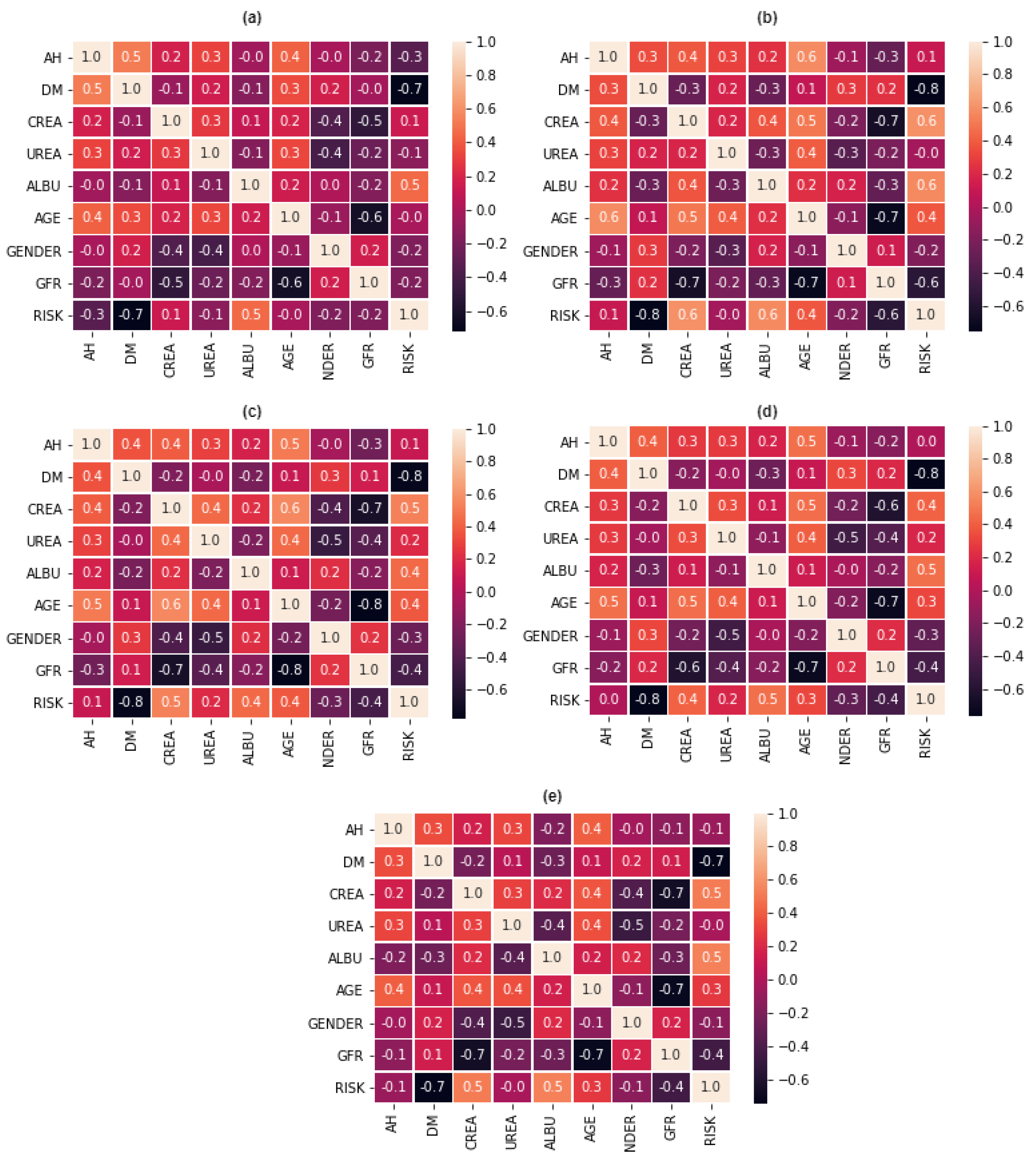
2.4. Multi-Class Feature Selection

As stated, we conducted manual data augmentation to improve the original dataset. Besides, we binarized the translated, preprocessed, and manually augmented dataset to enable the multi-class feature selection for implementing ensemble models. The multi-class feature selection included an additional data augmentation using SMOTE to balance each binary problem (low risk, moderate risk, high risk, and very high risk). We solve each binary problem with feature selection based on the framework proposed by Pineda-Bautista et al. [23]. The framework considers multi-class feature selection using class binarization and balancing. Thus, we applied the one-against-all class strategy and the SMOTE. Our main objective with the multi-class feature selection is to verify the importance of features and improve the ML ensemble models’ implementation. We used the ROC and PRC areas to conduct evaluations during the multi-class feature selection. Although ROC and PRC areas are typically used in binary classification, it is possible to extend them to evaluate multi-class classification problems using the one-against-all class strategy, as is the case of our multi-class feature selection. This enabled the definition of an ensemble model to solve our original multi-class problem by voting, trained based on the feature selection results for each binary problem.

2.5. Hold-Out Validation

We applied the hold-out method by splitting the original dataset into 70% for training and 30% for testing. For the manual augmentation, a dataset with 54 records, used in our previous study [5], was added to the training set composed of the original data, resulting in 96 records: low risk (51 records), moderate risk (18 records), high risk (24 records), and very high risk (3 records). We used the dataset generated by the manual augmentation for the automated augmentation and applied the SMOTE, Borderline-SMOTE, and Borderline-SMOTE SVM. The resampling using the SMOTE and Borderline-SMOTE resulted in 204 records, in which each class contained 51 records. The usage of Borderline-SMOTE SVM resulted in 181 records: low risk (51 records), moderate risk (51 records), high risk (51 records), and very high risk (28 records). The test sets, for all approaches, contained 18 records: low risk (7 records), moderate risk (1 record), high risk (8 records), and very high risk (2 records). The test set only contains non-augmented data. Thus, we only conducted data augmentation for the training set to ensure that the test set contained real data. We conducted comparisons using the following datasets: Only Manual Augmentation, Manual Augmentation + Augmentation with SMOTE, Manual Augmentation + Augmentation with Borderline-SMOTE, and Manual Augmentation + Augmentation with Borderline-SMOTE SVM.

2.6. Multiple Stratified Cross-Validation and Nested Cross-Validation

For the multiple stratified CV and nested CV methods, we split the original dataset into 10-folds, resulting in 54 records for training and 6 for testing. For the manual augmentation, we included 54 records in each of the 10-folds, in which each fold contained 108 data for training and 6 for testing. Training folds from 1 to 6 contained: low risk (55 records), moderate risk (18 records), high risk (30 records), and very high risk (5 records). The 7th-fold contained: low risk (55 records), moderate risk (17 records), high risk (31 records), and very high risk (5 records). From the 8th to 10th folds: low risk (55 records), moderate risk (18 records), high risk (31 records), and very high risk (4 records). We used the dataset generated by the manual augmentation for the automated augmentation and applied the SMOTE, Borderline-SMOTE, and Borderline-SMOTE SVM. The resampling using SMOTE and Borderline-SMOTE resulted in 220 records, in which all folds contained 55 records for each class. The Borderline-SMOTE SVM resulted in training folds, from 1st to 7th, with 196 records: low risk (55 records), moderate risk (55 records), high risk (55 records), and very high risk (31 records). Besides, from the 8th to 10th folds, it resulted in 195 records: low risk (55 records), moderate risk (55 records), high risk (55 records), and very high risk (30 records).

Besides investigating whether such methods satisfactorily control overfitting for our dataset (by comparison), in this article, the evaluation results are relevant to increase confidence in the ML model embedded in our developed DSS (Section 5—clinical context scenario). Therefore, they enabled us to evaluate the quality of our approach.

2.7. Algorithms

We experimented with supervised learning and the DT, RF, and multi-class AdaBoosted DTs classification models. We also apply methods for DCS (OLA and LCA) and methods for DES (KNORA-U, KNORA-E, and META-DES).

A DT uses the divide-and-conquer technique to solve classification and regression problems. It is an acyclic graph where each node is a division node or leaf node. The rules are based on information gain, which uses the concept of entropy to measure the randomness of a discrete random variable A (with domain $a_1,a_2,\dots ,a_n$) [37]. Entropy is used to calculate the difficulty of predicting the target attribute, where the entropy of A can be calculated by:

$$A=-\sum _{i=1}^n{p}_{i}lo{g}_2\left(p_i\right)$$

(1)

where, $p_i$ is the probability of observing each value $a_1,a_2,\dots ,a_n$. In the literature, DT has performed well with imbalanced datasets. Different algorithms generate the DT, such as ID3, C4.5, C5.0, and CART. The Scikit-learn library uses the CART algorithm.

The RF algorithm is used to combine DTs, generating several random trees. The algorithm assists modelers in preventing overfitting, being more robust when compared to a DT. It uses the Gini impurity criterion to conduct the feature selection, in which the following equation [38] guides the split of a node:

$$i\left(w\right)=\sum _{l=1}^L{p}_w^l(1-p_w^l)$$

(2)

where $p_j$ is the relative frequency of class j [33].

The multi-class AdaBoosted DTs algorithm creates a set of classifiers that contribute to the classification of test samples through weighted voting. With each new iteration, the weight of the training samples is changed considering the error of the set of classifiers previously implemented [37]. A multi-class AdaBoosted DTs performs the combination of predictions from all DTs in the set for multi-class problems.

Finally, a dynamic selection technique measures the performance level of each classifier in a classifier pool. If a classifier pool is not defined, a BaggingClassifier generates a pool containing 10 DTs. For the DCS method, the classifier that has achieved the highest performance level when classifying the samples in the test set is selected [22]. For the DES method, a set of classifiers that provide a minimum performance level is selected.

2.8. Classification Metrics

We computed the performance of the classification models using the python scikit-learn library [39] and the following metrics: precision, accuracy score, recall, balanced F score, MCC, ROC, and PRC. Precision represents the classifier’s ability of not label a sample incorrectly and is given by the equation:

$$Precision=\frac{TP}{TP+FP}$$

(3)

where, $TP$ represents the true positives and $FP$ represents the false positives. The accuracy score calculates the total performance of the model using the equation:

$$A(y,\widehat{y})=\frac{1}{n}\sum _{i=0}^{n-1}1(\widehat{y_i}=y_i)$$

(4)

where, $\widehat{y_i}$ represents the value that the model classified the sample, $y_i$ represents the real value of the sample, n is the total number of samples, and $I\left(x\right)$ is the indicator function [27].

The recall corresponds to the hit rate in the positive class and is given by

$$Recall=\frac{TP}{TP+FN}$$

(5)

where, $FN$ represents the false negatives. The balanced F-score or F measure is a weighted average between precision and recall:

$$F1=2\ast \frac{Precision\ast Recall}{Precision+Recall}$$

(6)

The MCC is used to assess the quality of ratings and is highly recommended for imbalanced data [40], given by the following equation:

$$MCC=\frac{TP\ast TN-FP\ast FN}{\sqrt{(TP+FP)(TP+FN)(TN+FP)(TN+FN)}}$$

(7)

where, $TN$ represents the true negative. Besides, the FMI is used to measure the similarity between two clusters, the measure varies between 0 and 1, where a high value indicates a good similarity [41]. FMI is defined as the geometric mean between precision and recall, given by the equation:

$$FMI=\sqrt{\frac{TP}{TP+FP}\ast \frac{TP}{TP+FN}}$$

(8)

The ROC calculates the probability estimates that a sample belongs to a specific class [42]. For multi-class problems, ROC uses two approaches: one-vs-one and one-vs-rest. Finally, the PRC is a widely used metric for imbalanced datasets that provides a clear visualization of the performance of a classifier [43].

3. Related Works

3.1. Early Prediction and DSS

ML models’ usage to assist in decision making has received the attention of researchers in the last years. For instance, Hsu [28] describes a framework based on a ranking and feature selection algorithm to assist physicians’ decision-making on cardiovascular diseases’ most relevant risk factors. The author also applies machine learning techniques to enable identifying the risk factors.

Walczak and Velanovich [29] developed an artificial neural network (ANN) system to assist physicians and patients in selecting pancreatic cancer treatment. The system determines the 7-month survival or mortality of patients based on a specific treatment decision. Topuz et al. [31] propose a decision support methodology guided by a Bayesian belief network algorithm to predict kidney transplantation’s graft survival. The authors use a database with more than 31,000 U.S. patients and argue that the methodology can be reused in other datasets.

Wang et al. [30] evaluate a murine model, induced by intravenous Adriamycin injection, using optical coherence tomography (OCT) to assess the CKD progression by images of rat kidneys. The authors highlight that OCT images contain relevant data about kidney histopathology. Jahantigh, Malmir, and Avilaq [32] propose a fuzzy expert system to assist the medical diagnosis, focusing initially on kidney diseases. The system is guided by the experience of physicians to indicate disease profiles. Neves et al. [34] present a DSS to identify acute kidney injury and CKD using knowledge representation and reasoning procedures based on logic programming and ANN. Polat et al. [33] used the support vector machine technique and the two-feature selection methods wrapper and filter to conduct the CKD identification early. The authors justify the computer-aided diagnosis based on high mortality rates of CKD. Finally, Arulanthu and Perumal [35] presented a DSS for CKD prediction (CKD or non-CKD) using a logistic regression model.

However, these CKD studies have some limitations. For example, relevant topics are the ML technique used to identify the disease and the costs of required examinations (predictors). Most of the studies use many predictors and apply complex analysis, increasing costs and making physician double-checking results problematic. Indeed, this type of functionality is relevant because other clinical conditions influence CKD, and the diagnosis is usually improved when physicians collaborate to conclude.

3.2. Oversampling Methods

As mentioned earlier, the growing use of ML in the medical field brings challenges such as limited and imbalanced data. Despite this, the use of such datasets can be quite relevant for the medical field [21] and studies have been carried out to deal with such limitations. Some methods use ML algorithms, probability, or weights to define the samples to be resampled, while some methods perform the combination of oversampling and undersampling [44]. Some of these works will be reported below.

One of the best-known techniques for dealing with this type of problem is SMOTE [34]. The purpose of SMOTE is to generate new synthetic minority class data, thus selecting a sample of the minority class randomly and its k nearest neighbors of the same class are calculated (by default 5) as a line is drawn around the selected samples and new synthetic data is generated.

Chawla et al. [34] performed a combination of subsampling and supersampling techniques. The subsampling technique was proposed in conjunction with supersampling to increase the sensitivity of a classifier to the minority class. Thus, in the proposed method, samples from the majority class were taken randomly and samples from the minority class were synthetically generated until it has a specific proportion of the majority class. In another work, Chawla et al. [45] performed a combination of the SMOTE algorithm with the boosting procedure, changing the update weights and compensating for skewed distributions of misclassified instances to generate synthetic data, thus creating the SMOTEBoost algorithm.

Unlike other methods that resample all examples from the minority class or that randomly select a subset, Han et al. [35] in their study, selects only the minority class samples that are Borderline and most likely to be misclassified, thus developing a variation of the SMOTE oversampling method called Borderline-SMOTE. While Nguyen and Kamei [36] used the SVM classifier to find the boundary region, combined with extrapolation and interpolation techniques for oversampling the minority boundary instances.

Das et al. [46] addressed two types of oversampling, namely, RACOG and wRACOG, where it used joint probability distribution of data attributes and Gibbs sampling to choose and generate the samples of minority classes synthetically. Wang [44] used the SMOTE oversampling method only to support minority class vectors that were found by training the cost-sensitive SVM classifier.

In contrast, we address very limited datasets by combining manual augmentation and automated augmentation. To verify the best combination, we experiment with manual augmentation along with automated augmentation using SMOTE, Borderline-SMOTE, and Borderline-SMOTE SVM.

3.3. Validation Methods

Some studies conduct comparisons of validation methods for ML models. For example, Varma and Simon [26] compared the multiple stratified CV and nested CV methods. The authors conclude that CV presents significantly biased estimates, in contrast with nested CV, that provides an almost unbiased estimate of the true error.

Moreover, Vabalas et al. [18] investigated whether bias, identified in some studies in the literature when reporting classification accuracy, could be caused by the use of specific validation methods. The authors also conclude that multiple stratified CV produces strongly biased performance estimates with small sample sizes. However, they also state that nested CV and hold-out present unbiased estimates. In another study, Varoquaux [47] also highlights the possibility of obtaining underestimated performance evaluation using CV.

Krstajic et al. [48] address best practices to improve reliability and confidence during the evaluation of ML models. The authors describe a repeated grid-search V-fold cross-validation approach and define a repeated nested cross-validation algorithm. They highlight the relevance of repeating cross-validation during model evaluation.

3.4. Comparison of ML Algorithms

Furthermore, some studies focus on the comparison of ML models to predict CKD. For example, Ilyas et al. [49] compared ML models for early prediction of CKD. They used the UCI machine learning repository, which consists of two classes (i.e., CKD affected and NOTCKD, indicating people with no CKD). However, the authors subdivide the CKD class into stages: Stage 1, Stage 2, Stage 3A, Stage 3B, Stage 4, and Stage 5. The prediction focuses on such stages.

Qin et al. [50] also used the UCI machine learning repository to assist the early detection of CKD as a binary problem. The authors apply KNN imputation to fill in the missing values of the dataset. They implemented ML models using logistic regression, RF, SVM, KNN, naive Bayes, and feed-forward neural network.

Chittora et al. [51] implemented ML models using ANN, C5.0, Chi-square Automatic interaction detector, logistic regression, linear SVM with penalty L1 and L2, and random tree. As a binary problem, the authors apply feature selection and oversampling techniques based on the UCI machine learning repository.

Chaurasia et al. [52] compared ensemble and non-ensemble models for the prediction of CKD as a binary problem. They evaluated the models using performance metrics such as accuracy rate, recall rate, F1 score, and support value. The ensemble models outperformed non-ensemble models.

4. Experiments

4.1. Statistical Significance

We conducted a correlation analysis to verify the relationship between the variables. Firstly, we analyze the correlation matrix generated through Person’s coefficients, where the measures vary between 1 and −1. On the one hand, a value closer to 1 indicates a strong correlation between two variables. On the other hand, a value close to −1 indicates an inverse correlation. The values are represented by means of colors. Thus, the lighter the color, the greater the correlation between the variables.

Figure 2 shows a sample of the correlation matrix coefficients using our CKD datasets. Figure 2a presents the correlation matrix from the dataset with the 60 real-world records and 54 manually augmented data. Samples of correlation matrix coefficients from the datasets related to the application of the hold-out method are also presented, with data further resampled with SMOTE (Figure 2b), borderline-SMOTE (Figure 2c), and borderline-SMOTE SVM (Figure 2d). Figure 2e presents the correlation matrix associated with the CV method with data further resampled with SMOTE. In general, the highest correlation coefficients relate to creatinine, urea, albuminuria, and age.

Moreover, we used linear regression to conduct a hypothesis test to verify statistical significance. We calculated the p-value to quantify statistical significance and analyze whether our hypothesis had any correlation between the features and the target. We consider a p-value < 0.05, as a strong relationship between the feature and the target. We also calculated the F-statistic to analyze the significance of the model implemented using the datasets (must be greater than 1). We used the R-Squared statistic to complement the analysis of the relationship between two variables, between 0 and 1 (indicates a strong correlation).

A sample of p-value, F-statistic, and R-Squared results is presented in Table S1 of Supplementary Materials. We identified a strong correlation between variables. For example, when using the dataset that relates to the application of the CV method, with data resampled using the manual approach and SMOTE, the null hypothesis was refuted for AH, DM, creatinine, albuminuria, and age. Besides, the F-statistic resulted in 126.90 and the R-Squared in 0.828, indicating a strong relationship between the variables and the target.

4.2. Implementation and Evaluation

We implemented the classification models using the DT, RF, and multi-class AdaBoosted DTs algorithms. Besides, we used dynamic selection methods: OLA, LCA, KNORA-E, KNORA-U, and META-DES. As mentioned before, we used the validation methods hold-out, multiple stratified CV, and nested CV, comparing resampling approaches: only manual augmentation, SMOTE, Borderline-SMOTE, and Borderline-SMOTE SVM. For the hold-out method, without the usage of the framework proposed by Pineda-Bautista et al. [23], dynamic selection (OLA, KNORA-E, and META-DES) and the DT model presented the highest performances using the mean values of precision (PR), accuracy score (ACC), recall, FMI, MCC, and F1 (e.g., with an equal ACC of 94.44% using the Borderline-SMOTE SVM). For the other resampling techniques, such models presented lower performances, with an ACC between 83.33% and 88.88%. We present such results in Table S2 of the Supplementary Materials. Due to the imbalance and limited size of the test set used for the hold-out method, we also applied the multiple stratified CV and nested CV as validation methods. Such methods evaluate the generalization of a model to a new dataset, using the whole data for training and testing.

Then, we applied the gridSearchCV tool with 5 repetitions for the multiple stratified CV and nested CV methods. We used such a tool to automate the combination of the best parameters and obtain the best performance from each algorithm. We used multiple stratified CV and nested CV with 10-folds and five repetitions. The multiple stratified CV method obtained a very similar result when compared to the nested CV, in some cases, with a difference of up to 6%. There is a difference because the multiple stratified CV uses the entire dataset to perform the best fit, producing optimistic performance estimates [53]. However, the nested CV splits the data into training, validation, and testing, using the gridSearchCV tool to set the best parameters only for the training data to produce unbiased performance estimates.

The DT, RF, and multi-class AdaBoosted DTs models presented stable results, obtaining high performance for all resampling methods. For multiple stratified CV and nested CV, the models achieved an ACC that ranged between 92.33% and 98.99%. The DT model presented the best performance, with an ACC of 98.99%, using SMOTE (see Tables S3 and S4 of our Supplementary Materials).

Furthermore, to improve the experiments, we implemented ensemble models based on the framework proposed by Pineda-Bautista et al. [23]. We split the original dataset into 70% for training and 30% for testing to select features from multiple classes. We improved the data using 38 records from the augmented dataset available in our public repository [32]. Afterward, we conducted the binarization of the training and test sets using the one-against-all classes strategy. We conducted the binarization for each class of our multi-class problem to obtain four different binary problems (low risk, moderate risk, high risk, and very high risk). We applied the SMOTE to handle imbalanced data for each binary problem; however, the usage of SMOTE did not improve the results. Finally, we used the CfsSubsetEval attribute evaluator and the BestFist research method to select the features of our binary problems. The feature selection results, for each binary problem, resulted in a maximum of five features for each class (

Table 3. Results of feature selection for each binary problem generated using the low risk, moderate risk, high risk, and very high risk classes.

Importance	Low	Moderate	High	Very High
1	AH	DM	AH	Crea
2	DM	Albu	DM	Age
3	Albu	-	Albu	GFR
4	Age	-	Age	-
5	GFR	-	Gender	-

).

The resulting ensemble model is composed of four submodels (one per class). Each submodel is trained based on the augmented dataset and the feature selection results for a specific class. Thus, each submodel may assign different classes to a new instance. To conduct the final classifications, we used the majority vote strategy.

We also applied the hold-out, multiple stratified CV, and nested CV validation methods for the ensemble models, comparing the resampling approaches: manual augmentation, SMOTE, Borderline-SMOTE, and Borderline-SMOTE SVM. In the hold-out validation method (

Table 4. Results for the hold-out method for the ensemble models implemented based on the framework proposed by Pineda-Bautista et al. [23].

	ACC	PR	Recall	Weighted F1	Macro F1	MCC	FMI
Manual Augmentation Only
Decision Tree	94.44	0.95	0.94	0.93	0.90	0.91	0.92
Random Forest	94.44	0.95	0.94	0.93	0.90	0.91	0.92
AdaBoosted DT	88.88	0.91	0.88	0.88	0.86	0.83	0.78
OLA	88.88	0.91	0.88	0.89	0.77	0.83	0.89
LCA	88.88	0.81	0.88	0.84	0.65	0.83	0.90
KNORA-U	88.88	0.81	0.88	0.84	0.65	0.83	0.90
KNORA-E	83.33	0.77	0.83	0.79	0.61	0.75	0.77
META-DES	83.33	0.80	0.83	0.80	0.59	0.75	0.82
Manual Augmentation + Augmentation with SMOTE
Decision Tree	94.44	0.95	0.94	0.93	0.90	0.91	0.92
Random Forest	94.44	0.95	0.94	0.93	0.90	0.91	0.92
AdaBoosted DT	94.44	0.95	0.94	0.93	0.90	0.91	0.91
OLA	88.88	0.89	0.88	0.88	0.84	0.83	0.84
LCA	88.88	0.91	0.88	0.89	0.77	0.83	0.89
KNORA-U	94.44	0.96	0.94	0.94	0.93	0.91	0.90
KNORA-E	94.44	0.97	0.94	0.95	0.90	0.92	0.91
META-DES	94.44	0.96	0.94	0.94	0.93	0.91	0.90
Manual Augmentation + Augmentation with Borderline-SMOTE
Decision Tree	94.44	0.95	0.94	0.93	0.90	0.91	0.92
Random Forest	88.88	0.91	0.88	0.88	0.86	0.83	0.78
AdaBoosted DT	88.88	0.89	0.88	0.88	0.86	0.82	0.80
OLA	88.88	0.89	0.88	0.88	0.84	0.83	0.84
LCA	88.88	0.91	0.88	0.88	0.86	0.83	0.78
KNORA-U	100.00	1.00	1.00	1.00	1.00	1.00	1.00
KNORA-E	94.44	0.95	0.94	0.93	0.90	0.91	0.91
META-DES	88.88	0.91	0.88	0.88	0.80	0.83	0.84
Manual Augmentation + Augmentation with Borderline-SMOTE SVM
Decision Tree	94.44	0.95	0.94	0.93	0.90	0.91	0.92
Random Forest	94.44	0.96	0.94	0.94	0.93	0.91	0.90
AdaBoosted DT	88.88	0.91	0.88	0.88	0.86	0.83	0.78
OLA	88.88	0.89	0.88	0.88	0.84	0.83	0.84
LCA	88.88	0.92	0.88	0.88	0.79	0.83	0.84
KNORA-U	88.88	88.88	88.88	88.88	0.84	0.82	0.84
KNORA-E	100.00	1.00	1.00	1.00	1.00	1.00	1.00
META-DES	94.44	0.96	0.94	0.94	0.93	0.91	0.90

), models implemented based on dynamic selection (KNORA-E and KNORA-U) and the DT algorithm presented the highest performances. KNORA-E and KNORA-U achieved the highest accuracy score for the Borderline-SMOTE SVM and Borderline-SMOTE resampling techniques, respectively. The DT model showed stability for all resampling techniques, with an accuracy score of 94.44%.

Finally, we applied the multiple stratified CV and nested CV validation methods, in which the DT and multi-class AdaBoosted DTs models demonstrated stability (the highest performances for all resampling methods). The multiple stratified CV method achieved an accuracy score between 95.00% and 97.66% (

Table 5. Results for the multiple stratified CV method for the ensemble models implemented based on the framework proposed by Pineda-Bautista et al. [23].

	ACC	PR	Recall	Weighted F1	Macro F1	MCC	FMI
Manual Augmentation Only
Decision Tree	95.66	0.92	0.95	0.93	0.90	0.93	0.94
Random Forest	91.00	0.84	0.91	0.87	0.80	0.86	0.87
AdaBoosted DT	95.00	0.93	0.95	0.93	0.91	0.93	0.91
OLA	90.33	0.84	0.90	0.86	0.79	0.86	0.88
LCA	87.33	0.80	0.87	0.82	0.74	0.81	0.83
KNORA-U	89.33	0.83	0.89	0.68	0.78	0.84	0.85
KNORA-E	91.33	0.85	0.91	0.87	0.81	0.87	0.88
META-DES	91.66	0.86	0.91	0.88	0.81	0.88	0.89
Manual Augmentation + Augmentation with SMOTE
Decision Tree	94.44	0.95	0.94	0.93	0.93	0.91	0.92
Random Forest	94.44	0.95	0.94	0.93	0.84	0.91	0.92
AdaBoosted DT	97.66	0.97	0.97	0.97	0.97	0.96	0.94
OLA	92.66	0.90	0.92	0.90	0.85	0.89	0.89
LCA	91.33	0.89	0.91	0.89	0.93	0.87	0.87
KNORA-U	94.99	0.94	0.95	0.94	0.89	0.93	0.94
KNORA-E	93.66	0.91	0.93	0.92	0.86	0.90	0.91
META-DES	93.33	0.92	0.93	0.92	0.87	0.90	0.89
Manual Augmentation + Augmentation with Borderline-SMOTE
Decision Tree	96.00	0.94	0.96	0.94	0.92	0.94	0.93
Random Forest	93.33	0.90	0.93	0.91	0.87	0.90	0.89
AdaBoosted DT	95.00	0.93	0.95	0.93	0.91	0.93	0.91
OLA	92.33	0.91	0.92	0.91	0.85	0.89	0.88
LCA	91.33	0.89	0.91	0.89	0.84	0.88	0.85
KNORA-U	94.33	0.93	0.94	0.93	0.88	0.92	0.93
KNORA-E	94.00	0.92	0.94	0.92	0.88	0.91	0.91
META-DES	94.33	0.93	0.94	0.93	0.87	0.92	0.93
Manual Augmentation + Augmentation with Borderline-SMOTE SVM
Decision Tree	96.66	0.94	0.96	0.95	0.92	0.95	0.95
Random Forest	91.66	0.87	0.91	0.88	0.85	0.88	0.84
AdaBoosted DT	95.33	0.93	0.95	0.93	0.91	0.93	0.92
OLA	88.88	0.89	0.88	0.88	0.85	0.83	0.84
LCA	90.66	0.85	0.90	0.87	0.80	0.86	0.87
KNORA-U	94.00	0.91	0.94	0.92	0.87	0.91	0.92
KNORA-E	93.33	0.92	0.93	0.92	0.86	0.90	0.91
META-DES	93.00	0.92	0.93	0.91	0.86	0.90	0.91

), while the nested CV method achieved an accuracy score between 94.98% and 96.66% (

Table 6. Results for the nested CV method for the ensemble models implemented based on the framework proposed by Pineda-Bautista et al. [23].

	ACC	PR	Recall	Weighted F1	Macro F1	MCC	FMI
Manual Augmentation Only
Decision Tree	95.66	0.94	0.95	0.93	0.90	0.93	0.94
Random Forest	91.66	0.85	0.91	0.88	0.81	0.87	0.88
AdaBoosted DT	95.00	0.93	0.95	0.93	0.91	0.93	0.91
OLA	89.00	0.82	0.89	0.85	0.77	0.84	0.87
LCA	83.99	0.75	0.84	0.78	0.69	0.76	0.78
KNORA-U	88.00	0.81	0.88	0.83	0.76	0.82	0.84
KNORA-E	91.66	0.87	0.91	0.89	0.82	0.87	0.88
META-DES	90.00	0.83	0.90	0.86	0.78	0.85	0.87
Manual Augmentation + Augmentation with SMOTE
Decision Tree	94.98	0.92	0.94	0.93	0.90	0.92	0.91
Random Forest	90.00	0.85	0.90	0.86	0.80	0.85	0.84
AdaBoosted DT	96.66	0.94	0.96	0.95	0.93	0.95	0.95
OLA	92.66	0.92	0.92	0.91	0.85	0.89	0.90
LCA	91.33	0.89	0.91	0.89	0.85	0.87	0.85
KNORA-U	92.66	0.92	0.92	0.91	0.86	0.86	0.89
KNORA-E	90.00	0.88	0.90	0.88	0.80	0.89	0.85
META-DES	92.66	0.90	0.92	0.91	0.85	0.89	0.90
Manual Augmentation + Augmentation with Borderline-SMOTE
Decision Tree	96.00	0.93	0.94	0.94	0.92	0.94	0.93
Random Forest	92.66	0.89	0.92	0.90	0.85	0.89	0.88
AdaBoosted DT	96.66	0.95	0.96	0.95	0.93	0.95	0.94
OLA	90.00	0.88	0.90	0.88	0.82	0.85	0.83
LCA	90.66	0.88	0.90	0.89	0.83	0.87	0.85
KNORA-U	92.33	0.91	0.92	0.91	0.85	0.89	0.89
KNORA-E	92.66	0.91	0.92	0.91	0.85	0.89	0.90
META-DES	92.66	0.90	0.92	0.90	0.84	0.89	0.90
Manual Augmentation + Augmentation with Borderline-SMOTE SVM
Decision Tree	91.33	0.89	0.92	0.88	0.82	0.87	0.86
Random Forest	90.66	0.85	0.90	0.87	0.82	0.86	0.84
AdaBoosted DT	92.66	0.90	0.92	0.90	0.86	0.89	0.87
OLA	90.33	0.86	0.90	0.87	0.81	0.86	0.85
LCA	88.66	0.84	0.88	0.85	0.79	0.84	0.82
KNORA-U	92.66	0.91	0.92	0.91	0.86	0.89	0.89
KNORA-E	91.33	0.89	0.91	0.89	0.82	0.87	0.88
META-DES	93.00	0.92	0.93	0.91	0.86	0.90	0.91

).

As stated above, our comparisons also considered the results without using the framework proposed by Pineda-Bautista et al. [23] (see Tables S2–S4 of our Supplementary Materials). To summarize our findings, we present the decision tree results (from Tables S2–S4 of our Supplementary Materials) in

Table 7. Decision tree results for the hold-out, multiple stratified CV, and nested CV methods without using the framework proposed by Pineda-Bautista et al. [23].

	ACC	PR	Recall	Weighted F1	Macro F1	MCC	FMI
Manual Augmentation Only
Hold-out	83.33	0.77	0.83	0.79	0.61	0.74	0.77
Multiple stratified CV	92.33	0.92	0.92	0.91	0.88	0.90	0.86
Nested CV	92.33	0.92	0.92	0.91	0.90	0.90	0.82
Manual Augmentation + Augmentation with SMOTE
Hold-out	83.33	0.86	0.83	0.84	0.80	0.74	0.78
Multiple stratified CV	98.99	0.99	0.99	0.98	0.98	0.98	0.98
Nested CV	98.99	1.00	0.99	0.99	0.98	0.98	0.99
Manual Augmentation + Augmentation with Borderline-SMOTE
Hold-out	88.88	0.88	0.88	0.88	0.84	0.82	0.84
Multiple stratified CV	98.00	0.98	0.98	0.97	0.96	0.97	0.98
Nested CV	95.00	0.95	0.95	0.95	0.94	0.93	0.88
Manual Augmentation + Augmentation with Borderline-SMOTE SVM
Hold-out	94.44	0.95	0.94	0.93	0.90	0.91	0.91
Multiple stratified CV	95.00	0.93	0.95	0.93	0.91	0.93	0.91
Nested CV	96.00	0.94	0.96	0.95	0.91	0.94	0.95

.

Besides, we calculated the ROC and PRC curves using a one-against-all classes strategy. We identified the trade-offs between sensitivity (true positive rate) and specificity (true negative rate) to show the model’s diagnostic abilities using the ROC area. For example, for the ROC curve performance of the DT model, which relates to the usage of SMOTE and the nested CV methods, high discriminatory power was achieved for all folds. One can also identify that the curves are closer to the upper left corner of each graphic (Figure 3 and Figure 4). In addition, the PRC area shows the relationship between accuracy and recall and is relevant to analyze imbalanced datasets (see Figures S1–S3 of our Supplemental Materials). The precision-recall curve shows the trade-off between precision and recall for different thresholds. For the performance of the DT model, which is related to the use of SMOTE and nested CV methods, high discriminatory power was achieved for all folds, increasing confidence in the results presented with ROC curves. The source codes of the experiments are available in our repository [54].

5. Clinical Practice Context

Using eHealth and mHealth systems to aid in the treatment and identification of chronic diseases can be one way to reduce high mortality rates through monitoring chronic diseases such as CKD. This situation refers to using information and technologies intelligently and effectively to guide those whom public health systems will eventually assist. Early computer-aided identification of CKD can help people living in the countryside and environments with difficult access to primary care. In addition, mobile health apps (i.e., mHealth), which generate personal health records (PHR), can be used to reduce issues (i.e., store a patient’s complete medical history with diagnosis, administered medications, plans for treatment, vaccination dates, allergies) related to primary health care in remote locations.

Therefore, the presented classification models can be used to develop eHealth and mHealth systems that assist patients, clinicians, and the government in monitoring CKD and its risk factors. Using the Brazilian CKD dataset, we recommend applying the DT model with data resampled with the SMOTE technique to develop a DSS. The DT model achieved high performance, and it is considered a white box analysis approach with a straightforward interpretation of results. Interpreting the results helps doctors understand how the model achieved a specific risk rating, increasing these professionals’ confidence in the results.

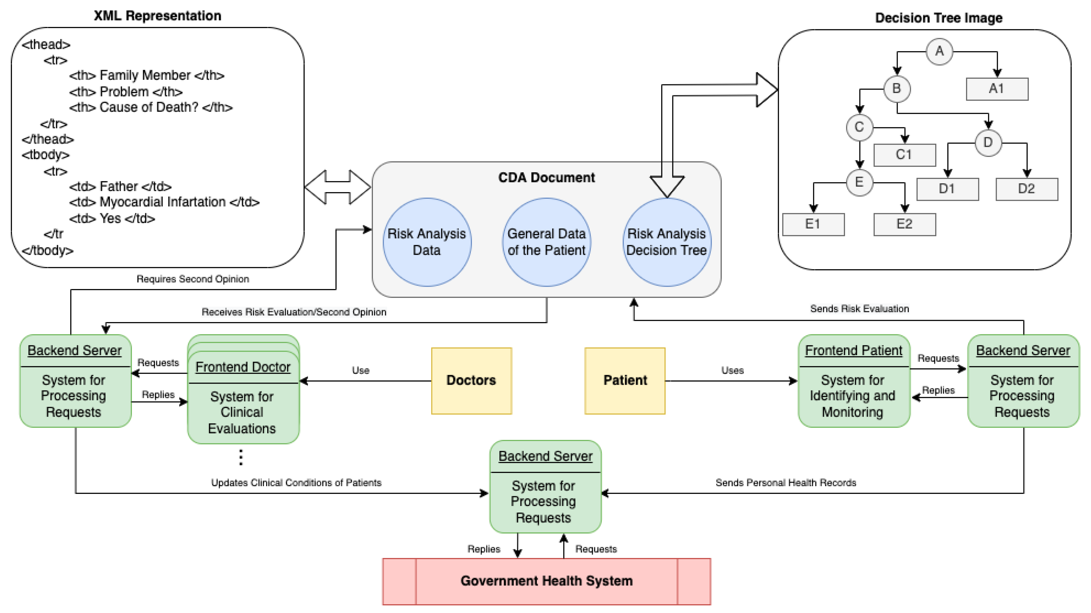
The ML model can be the basis for developing a DSS to identify and monitor CKD in Brazilian communities, where the interaction between three actors is proposed: doctor, patient, and public health system (Figure 5). The system used by patients is presented as a web-based system divided into front-end and back-end, which contains PHR and CKD risk assessment functionality. The risk assessment is performed after inputting the results of exams, where the classification of risk of CKD is based on the DT model. After the user’s clinical evaluation, the system can send a clinical document, structured from the HL7 clinical document architecture (CDA) to the doctor responsible for monitoring the patient. The HL7 CDA document is an XML file that contains the risk analysis data, a risk analysis DT, and the PHR.

The medical system receives the CDA document to confirm the risk assessment by analyzing the classification, the DT, and the PHR data. In an uncertain diagnosis, the doctor can send the CDA document to other doctors for a second opinion. The patient and medical subsystems use web services provided by the Server subsystem to update the PHR of patients as part of the medical records available at a healthcare facility. We provide a more detailed explanation of this type of system for CKD and related technologies in our previous publication [28].

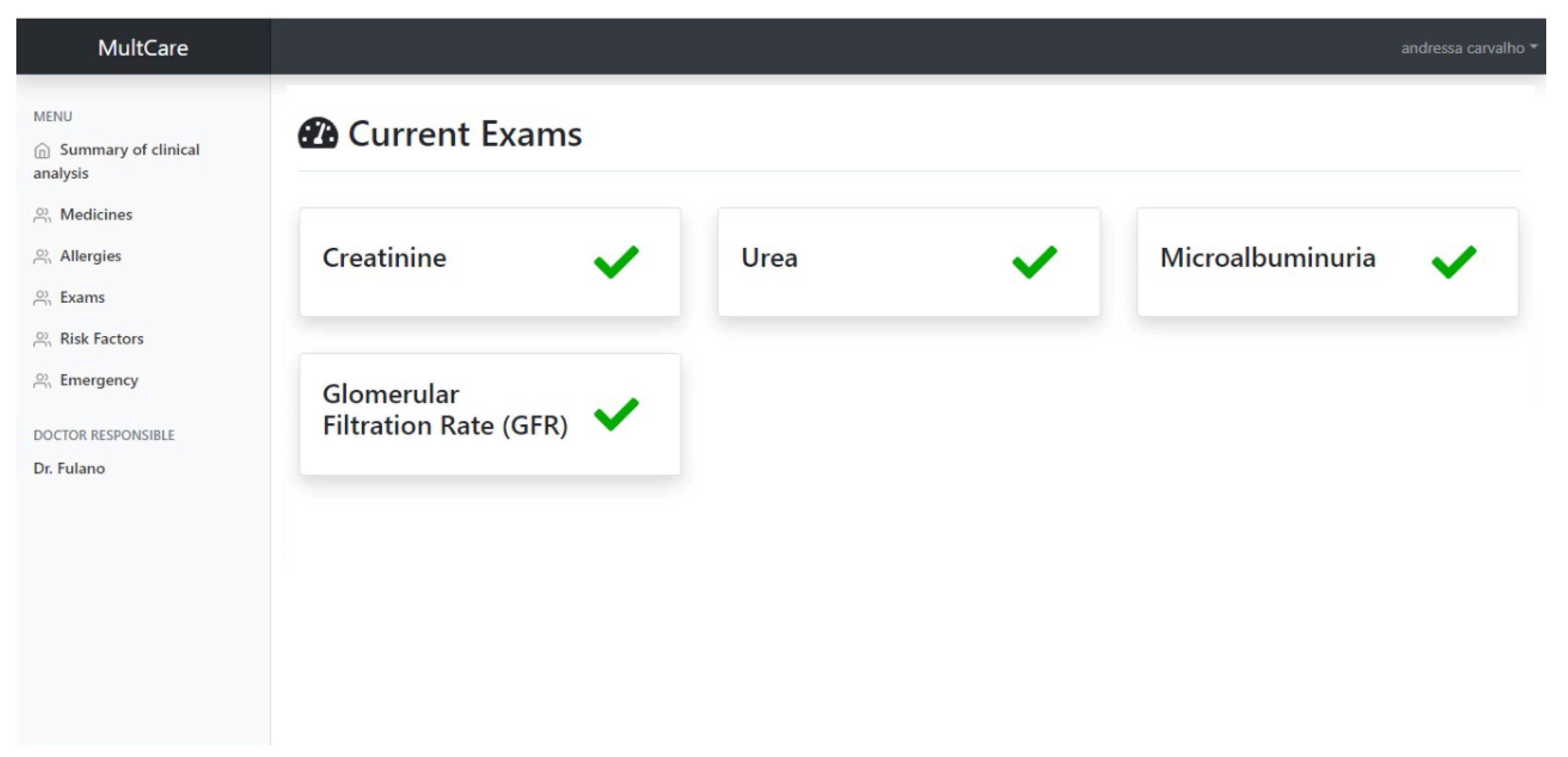
Therefore, we implemented a web-based application considering the system used by patients, as an improvement of the results presented in [28]. The back-end of such subsystem was implemented using the Java programming language and web services. The subsystem comprises the following main features: access control, management of ingested drugs, management of allergies, management of examinations, monitoring of hypertension and DM, execution of risk analysis, generation and sharing CDA documents, and analysis of the emergency. In contrast, the front-end of the subsystem is implemented using HTML 5, Bootstrap, JavaScript, and Vue.js. For the graphical user interface (GUI) for recording a new CKD test result (the main inputs for the risk assessment model), the user can also upload an XML file containing the test results to present a large number of manual inputs. Once the patient provides the current test results, the main GUI of the subsystem is updated, showing the test results available for the risk assessment.

Figure 6 illustrates the main GUI of the patient sub-system, describing the creatinine, urea, albuminuria, and GFR (i.e., the main attributes used by the risk assessment model). This study reduces the number of required test results to conduct the CKD risk analysis from 5 to 4 compared to the previously published research [16]. This is critical for low-income populations using the sub-system because a very large number of biomarkers increases costs, that usually cannot be afforded by such people. Indeed, a reduced number of biomarkers can include more users for this type of DSS that would be possibly excluded due to their limited financial resources. The sub-system provides a new CKD risk analysis when the patient inputs all CKD attributes.

During the CKD risk analysis (conducted when all tests are available), and based on the presence/absence of DM, presence/absence of hypertension, age, and gender, the J48 decision tree algorithm classifies the patient’s situation considering four classes: low risk, moderate risk, high risk, and very high risk. In case of moderate risk, high risk, or very high risk, the sub-system packages the classification results as a CDA document, along with the decision tree graphic and general data of the patient. The sub-system alerts the physician responsible for the patient and sends the complete CDA document (i.e., the main output of the DSS) for further clinical analysis. In the case of low risk, the sub-system only records the risk analysis results to keep track of the patient’s clinical situation. It does not send the physician alert, automating the risk analysis and sharing. This illustrates an example of scenario that shows how the definition of risk levels can provide more details on the patients’ clinical conditions.

Results presented in this article justify the usage of the DT algorithm and attributes (i.e., presence/absence of DM, presence/absence of AH, creatinine, urea, albuminuria, age, gender, and GFR) to conduct risk analyses in developing countries. The physician responsible for the healthcare of a specific patient can, remotely, access the CDA document by a medical sub-system, re-evaluate or confirm the risk analysis (i.e., preliminary diagnosis) provided by the patient sub-system, and share the data with other physicians to get second opinions. If the physician confirms the preliminary diagnosis, the patient can continue using the patient sub-system to prevent the CKD progression, including the monitoring of risk factors (DM and AH), CKD stage, and risk level.

We also implemented the medical and server sub-systems using web technologies based on Figure 5. However, the description of such sub-systems is not in the scope of this article.

6. Discussion

When dealing with imbalanced and limited-size datasets, the evaluation of resampling and validation methods is essential to verify the stability of ML models. Our results indicated the non-ensemble DT model with data resampled with manual augmentation + SMOTE, with the best performance, obtaining a mean accuracy score of 98.99% for multiple stratified CV (see Table S2 of our Supplementary Materials) and nested CV (see Table S3 of our Supplementary Materials). The DT is followed by the multi-class AdaBoosted DTs model with a mean accuracy score of 97.99% for multiple stratified CV (see Table S2 of our Supplementary Materials) and 98% for nested CV (see Table S3 of our Supplementary Materials).

During CKD monitoring, based on the non-ensemble DT model with data resampled with manual augmentation + SMOTE, assuming the previous DM evaluation, the user only needs to perform two blood tests: creatinine and urea periodically. Albuminuria is measured using a urine test, while GFR can be calculated using the Cockcroft-Gault equation. The reduced number of exams is relevant for developing countries like Brazil due to the high poverty levels.

From the misclassified instances identified when testing the non-ensemble DT model, with data resampled with manual augmentation + SMOTE, the model disagreed with the experienced nephrologist, declaring very high risk rather than high risk (only one individual). However, the model did not lead to any critical underestimation of individuals’ at-risk status (e.g., low risk rather than moderate risk). This situation would be a critical issue because the patient is usually referred to a nephrologist at moderate or high risk. Misleading classifications are less harmful to the patient as they still result in the patient being referred for evaluation, even if the risk is overestimated.

Along with using a reduced number of features and the absence of critical underestimations, another advantage of the DT model is the direct interpretation of results. A more straightforward interpretation of the CKD risk analysis by nephrologists and primary care doctors who need to perform additional tests to confirm a patient’s clinical status is critical to reusing the model in real-world situations. The tree generated by the DT model encompasses each CKD biomarker considered and the related classification. A doctor follows the decisions to interpret the logic of classification. Of the 8 CKD features, only 5 were used by the non-ensemble DT model with data resampled with manual augmentation + SMOTE, to classify the risk (i.e., creatinine, gender, HA, urea, and albuminuria), requiring one blood test and one urine test when DM has already been evaluated, at the cost of one misclassified instance.

However, one of the main limitations of this study is the usage of the gridSearchCV tool to find the best parameters for each algorithm. We faced processing limitations, mainly for the ensemble models, because the parameter search was conducted for each ML model. The usage of gridSearchCV with 5 folds for the DT model is one example of such a situation. We handled 960 candidates, resulting in 4800 adjustments. However, when using the META-DES model, we handle 8640 candidates, resulting in 43,200 adjustments for the ensemble model, presenting a higher processing cost to adjust the parameters.

Besides, the reduced amount of manually augmented instances may also be considered a limitation. For example, the number of instances for the very high risk class in the test set is too reduced, which can have a negative impact on the performance evaluation for such class. The nested CV assisted us in reducing this limitation. We did not provide more augmented data because it is a time-consuming task for the nephrologist. However, given that one of the main purposes of this study is to address limited size datasets, the manual augmentation provided by the nephrologist was enough to conduct the experiments.

7. Conclusions and Future Work

The approach presented in this article can help design DSS to identify CKD in Brazilian communities. Such a system is relevant because low-income populations in Brazil generally suffer from the lack/precariousness of primary care. We develop and evaluate ensemble and non-ensemble models using different data resampling techniques for our CKD datasets. The result of the DT model with data resampled with the SMOTE technique improves the results of previous works. The remote identification of chronic diseases through DSS is even more relevant, considering the epidemics that prevent face-to-face care. For example, in Brazil, the COVID-19 epidemic negatively impacted the health assistance of low-income populations with chronic diseases, increasing mortality rates.

As future work, we envision applying formal modeling languages, such as coloured Petri nets, aiming to improve the accuracy of decision rules extracted from ML models. The formal modeling of decision rules is relevant, for example, to solve conflicting rules.

References

1. Bikbov, B.; Purcell, C.A.; Levey, A.S.; Smith, M.; Abdoli, A.; Abebe, M.; Adebayo, O.M.; Afarideh, M.; Agarwal, S.K.; Agudelo-Botero, M.; et al. Global, regional, and national burden of chronic kidney disease, 1990–2017: A systematic analysis for the global burden of disease study 2017. Lancet 2020, 395, 709–733. [Google Scholar] [CrossRef] [Green Version]
2. Abegunde, D.; Stanciole, A. Preventing Chronic Diseases: A Vital Investment: Who Global Report; World Health Organization: Geneva, Switzerland, 2006.
3. World Health Organization. World Health Statistics Overview 2019: Monitoring Health for the SDGS, Sustainable Development Goals; World Health Organization: Geneva, Switzerland, 2019.
4. Sociedade Brasileira de Diabetes. Guidelines of the Brazilian Society of Diabetes 2019–2020; Sociedade Brasileira de Diabetes: São Paulo, Brazil, 2019. [Google Scholar]
5. Sobrinho, A.; Queiroz, A.C.M.D.S.; Silva, L.D.D.; Costa, E.D.B.; Pinheiro, M.E.; Perkusich, A. Computer-aided diagnosis of chronic kidney disease in developing countries: A comparative analysis of machine learning techniques. IEEE Access 2020, 8, 25407–25419. [Google Scholar] [CrossRef]
6. Levey, A.; Inker, L.; Coresh, J. Chronic kidney disease in older people. J. Am. Med. Assoc. 2015, 314, 557–558. [Google Scholar] [CrossRef] [PubMed]
7. Kinaan, M.; Yau, H.; Martinez, S.Q.; Kar, P. Concepts in diabetic nephropathy: From pathophysiology to treatment. J. Ren. Hepatic Disord. 2017, 1, 10–24. [Google Scholar] [CrossRef]
8. Sesso, R.C.C.; Lopes, A.A.; Thomé, F.S.; Lugon, J.R.; Burdmann, E.A. Brazilian dialysis census 2009. Braz. J. Nephrol. 2010, 32, 380–384. [Google Scholar] [CrossRef] [Green Version]
9. Webster, A.C.; Nagler, E.V.; Morton, R.L.; Masson, P. Chronic kidney disease. Lancet 2017, 389, 1238–1252. [Google Scholar] [CrossRef]
10. Sesso, R.C.; Lopes, A.A.; Thomé, F.S.; Lugon, J.R.; dos Santos, D.R. 2010 report of the brazilian dialysis census. Braz. J. Nephrol. 2011, 33, 442–447. [Google Scholar] [CrossRef] [Green Version]
11. Sesso, R.C.; Lopes, A.A.; Thomé, F.S.; Lugon, J.R.; Martins, C.T. Brazilian chronic dialysis survey 2016. Braz. J. Nephrol. 2017, 39, 380–384. [Google Scholar] [CrossRef]
12. Thomé, F.S.; Sesso, R.C.; Lopes, A.A.; Lugon, J.R.; Martins, C.T. Brazilian chronic dialysis survey 2017. Braz. J. Nephrol. 2019, 41, 208–214. [Google Scholar] [CrossRef] [Green Version]
13. Neves, P.D.M.M.; Sesso, R.C.C.; Thomé, F.S.; Lugon, J.R.; Nascimento, M.M. Brazilian dialysis census: Analysis of data from the 2009–2018 decade. Braz. J. Nephrol. 2020, 42, 191–200. [Google Scholar] [CrossRef]
14. Chan, C.T.; Blankestijn, P.J.; Dember, L.M.; Gallieni, M.; Harris, D.C.; Lok, C.E.; Mehrotra, R.; Stevens, P.E.; Wang, A.Y.M.; Cheung, M.; et al. Dialysis initiation, modality choice, access, and prescription: Conclusions from a Kidney Disease: Improving Global Outcomes (KDIGO) Controversies Conference. Kidney Int. 2019, 96, 37–47. [Google Scholar] [CrossRef] [PubMed] [Green Version]
15. Elshahat, S.; Cockwell, P.; Maxwell, A.P.; Griffin, M.; O’Brien, T.; O’Neill, C. The impact of chronic kidney disease on developed countries from a health economics perspective: A systematic scoping review. PLoS ONE 2020, 15, e0230512. [Google Scholar] [CrossRef] [PubMed] [Green Version]
16. Brazilian Ministry of Health. Available online: https://bit.ly/3uNAS3Y (accessed on 1 April 2020).
17. Cha’on, U.; Wongtrangan, K.; Thinkhamrop, B.; Tatiyanupanwong, S.; Limwattananon, C.; Pongskul, C.; Panaput, T.; Chalermwat, C.; Lert-Itthiporn, W.; Sharma, A.; et al. Ckdnet, a quality improvement project for prevention and reduction of chronic kidney disease in the northeast Thailand. BMC Public Health 2020, 20, 1–11. [Google Scholar] [CrossRef] [PubMed]
18. Vabalas, A.; Gowen, E.; Poliakoff, E.; Casson, A.J. Machine learning algorithm validation with a limited sample size. PLoS ONE 2019, 14, e0224365. [Google Scholar] [CrossRef] [PubMed]
19. Sun, Y.; Wong, A.K.C.; Kamel, M.S. Classification of imbalanced data: A review. Int. J. Pattern Recognit. Artif. Intell. 2009, 23, 687–719. [Google Scholar] [CrossRef]
20. Jeni, L.A.; Cohn, J.F.; De La Torre, F. Facing imbalanced data–recommendations for the use of performance metrics. In Proceedings of the 2013 Humaine Association Conference on Affective Computing and Intelligent Interaction, Geneva, Switzerland, 2–5 September 2013; pp. 245–251. [Google Scholar]
21. Choi, M.Y.; Christopher, M. Making a big impact with small datasets using machine-learning approaches. Lancet Rheumatol. 2020, 2, e451–e452. [Google Scholar] [CrossRef]
22. Cruz, R.M.O.; Hafemann, L.G.; Sabourin, R.; Cavalcanti, G.D.C. DESlib: A Dynamic ensemble selection library in Python. J. Mach. Learn. Res. 2020, 21, 1–5. [Google Scholar]
23. Pineda-Bautista, B.B.; Carrasco-Ochoa, J.; Martınez-Trinida, J.F. General framework for class-specific feature selection. Expert Syst. Appl. 2011, 38, 10018–10024. [Google Scholar] [CrossRef]
24. Hulse, J.V.; Khoshgoftaar, T.M.; Napolitano, A. Experimental perspectives on learning from imbalanced data. In Proceedings of the 24th International Conference on Machine Learning, Corvallis, OR, USA, 20–24 June 2007; pp. 935–942. [Google Scholar]
25. Akbani, R.; Kwek, S.; Japkowicz, N. Applying support vector machines to imbalanced datasets. In Proceedings of the European Conference on Machine Learning, Pisa, Italy, 20–24 September 2004; pp. 39–50. [Google Scholar]
26. Varma, S.; Simon, R. Bias in error estimation when using cross-validation for model selection. BMC Bioinform. 2006, 7, 1–8. [Google Scholar] [CrossRef] [Green Version]
27. Santos Santana, Í.V.; Silveira, A.C.; Sobrinho, Á.; e Silva, L.C.; da Silva, L.D.; Santos, D.F.; Gurjão, E.C.; Perkusich, A. Classification Models for COVID-19 Test Prioritization in Brazil: Machine Learning Approach. J. Med. Internet Res. 2021, 23, e27293. [Google Scholar] [CrossRef]
28. Sobrinho, A.; da Silva, L.D.; Perkusich, A.; Pinheiro, M.E.; Cunha, P. Design and evaluation of a mobile application to assist the self-monitoring of the chronic kidney disease in developing countries. BMC Med. Informatics Decis. Mak. 2018, 18, 1–14. [Google Scholar] [CrossRef] [PubMed]
29. Lamb, E.J.; Levey, A.S.; Stevens, P.E. The kidney disease improving global outcomes (KDIGO) guideline update for chronic kidney disease: Evolution not revolution. Clin. Chem. 2013, 59, 462–465. [Google Scholar] [CrossRef] [PubMed]
30. Forbes, A.; Gallagher, H. Chronic kidney disease in adults: Assessment and management. Clin. Med. 2020, 2020, 128–132. [Google Scholar] [CrossRef] [PubMed] [Green Version]
31. Inker, L.A.; Astor, B.C.; Fox, C.H.; Isakova, T.; Lash, J.P.; Peralta, C.A.; Tamura, M.K.; Feldman, H.I. KDOQI US commentary on the 2012 KDIGO clinical practice guideline for the evaluation and management of CKD. Am. J. Kidney Dis. 2014, 63, 713–735. [Google Scholar] [CrossRef] [PubMed] [Green Version]
32. Sobrinho, A.; da Silva, L.D.; Perkusich, A.; Queiroz, A.; Pinheiro, M.E. A Brazilian Dataset for Screening the Risk of the Chronic Kidney Disease. Available online: https://bit.ly/3rQxllg (accessed on 1 April 2022).
33. Lemaître, G.; Nogueira, F.; Aridas, C.K. Imbalanced-learn: Apython toolbox to tackle the curse of imbalanced datasets in machine learning. J. Mach. Learn. Res. 2017, 18, 1–5. [Google Scholar]
34. Chawla, N.V.; Bowyer, K.W.; Hall, L.O.; Kegelmeyer, W.P. SMOTE: Synthetic minority over-sampling technique. J. Artif. Intell. Res. 2002, 16, 321–357. [Google Scholar] [CrossRef]
35. Han, H.; Wang, W.-Y.; Mao, B.-H. Borderline-smote: A new over-sampling method in imbalanced datasets learning. In Proceedings of the International Conference on Intelligent Computing, Hefei, China, 23–26 August 2005; pp. 878–887. [Google Scholar]
36. Nguyen, H.M.; Cooper, E.W.; Kamei, K. Borderline over-sampling for imbalanced data classification. J. Knowl. Eng. Soft Data Paradig. 2011, 3, 4–21. [Google Scholar]
37. Bishop, C.M. Pattern Recognition and Machine Learning, 2nd ed.; Springer: Berlin/Heidelberg, Germany, 2011. [Google Scholar]
38. Langs, G.; Menze, B.H.; Lashkari, D.; Golland, P. Detecting stable distributed patterns of brain activation using gini contrast. NeuroImage 2011, 56, 497–507. [Google Scholar] [CrossRef] [Green Version]
39. Pedregosa, F.; Varoquaux, G.; Gramfort, A.; Michel, V.; Thirion, B.; Grisel, O.; Blon-del, M.; Prettenhofer, P.; Weiss, R.; Dubourg, V.; et al. Scikit-learn: Machine learning in Python. J. Mach. Learn. Res. 2011, 12, 2825–2830. [Google Scholar]
40. Boughorbel, S.; Jarray, F.; El-Anbari, M. Optimal classifier for imbalanced data using Matthews Correlation Coefficient metric. PLoS ONE 2017, 12, e0177678. [Google Scholar] [CrossRef]
41. Fowlkes, E.B.; Mallows, C.L. A Method for Comparing Two Hierarchical Clusterings. J. Am. Stat. Assoc. 2012, 78, 553–569. [Google Scholar] [CrossRef]
42. Hand, D.J.; Till, R.J. A Simple Generalisation of the Area Under the ROC Curve for Multiple Class Classification Problems. Mach. Learn. 2001, 45, 171–186. [Google Scholar] [CrossRef]
43. Davis, J.; Goadrich, M. The relationship between Precision-Recall and ROC curves. In Proceedings of the 23rd International Conference on Machine Learning, Pittsburgh, PA, USA, 25–29 June 2006. [Google Scholar]
44. Wang, H.Y. Combination approach of SMOTE and biased-SVM for imbalanced datasets. In Proceedings of the IEEE International Joint Conference on Neural Networks (IEEE World Congress on Computational Intelligence), Hong Kong, China, 1–6 June 2008. [Google Scholar]
45. Chawla, N.V.; Lazarevic, A.; Hall, L.O.; Bowyer, K.W. SMOTEBoost: Improving Prediction of the Minority Class in Boosting. In Proceedings of the European Conference on Principles of Data Mining and Knowledge Discovery, Helsinki, Finland, 19–23 August 2003. [Google Scholar]
46. Das, B.; Krishnan, N.C.; Cook, D.J. RACOG and wRACOG: Two Probabilistic Oversampling Techniques. IEEE Trans. Knowl. Data Eng. 2015, 27, 222–234. [Google Scholar] [CrossRef] [PubMed] [Green Version]
47. Varoquaux, G. Cross-validation failure: Small sample sizes lead to large error bars. NeuroImage 2018, 180, 68–77. [Google Scholar] [CrossRef] [PubMed] [Green Version]
48. Krstajic, D.; Buturovic, L.J.; Leahy, D.E.; Thomas, S. Cross-validation pitfalls when selecting and assessing regression and classification models. J. Cheminform. 2014, 6, 1–15. [Google Scholar] [CrossRef] [Green Version]
49. Ilyas, H.; Ali, S.; Ponum, M.; Hasan, O.; Mahmood, M.T.; Iftikhar, M.; Malik, M.H. Chronic kidney disease diagnosis using decision tree algorithms. BMC Nephrol. 2021, 22, 1–11. [Google Scholar] [CrossRef]
50. Qin, J.; Chen, L.; Liu, Y.; Liu, C.; Feng, C.; Chen, B. A Machine Learning Methodology for Diagnosing Chronic Kidney Disease. IEEE Access 2020, 8, 20991–21002. [Google Scholar] [CrossRef]
51. Chittora, P.; Chaurasia, S.; Prasun, C.; Kumawat, G.; Chakrabarti, T.; Leonowicz, Z.; Jasiński, M.; Jasiński, Ł.; Gono, R.; Jasińska, E.; et al. Prediction of Chronic Kidney Disease—A Machine Learning Perspective. IEEE Access 2021, 9, 17312–17334. [Google Scholar] [CrossRef]
52. Chaurasia, V.; Pandey, M.K.; Pal, S. Chronic kidney disease: A prediction and comparison of ensemble and basic classifiers performance. Hum. Intell. Syst. Integr. 2022, 1–10. [Google Scholar] [CrossRef]
53. Abdulaal, M.; Casson, A.; Gaydecki, P. Performance of Nested vs. Non-nested SVM Cross-validation Methods in Visual BCI: Validation Study. In Proceedings of the 2018 26rd European Signal Processing Conference (EUSIPCO), Rome, Italy, 3–7 September 2018. [Google Scholar]
54. CKD-Experiment. Available online: https://bit.ly/3BpnsOw (accessed on 1 April 2022).
Figure 2. Sample of correlation matrix coefficients. (a) Dataset with the 60 real-world records and 54 manually augmented data. (b) Dataset with the application of the hold-out method and data further resampled with SMOTE. (c) Dataset with the application of the hold-out method and data further resampled with borderline-SMOTE. (d) Dataset with the application of the hold-out method and data further resampled with borderline-SMOTE SVM. (e) Dataset with CV method with data further resampled with SMOTE.
Applsci 12 03673 g002
Figure 3. ROC curves of the DT model using SMOTE and the nested CV method for the five first folds. Each graphic represents one of the ten folds.
Applsci 12 03673 g003
Figure 4. ROC curves of the DT model using SMOTE and the nested CV method for the sixth, seventh, eighth, ninth, and tenth folds. Each graphic represents one of the ten folds.
Applsci 12 03673 g004
Figure 5. DSS methodology schema of identification and monitoring of CKD in developing countries.
Applsci 12 03673 g005
Figure 6. Screenshot of the main GUI for the patient sub-system.
Applsci 12 03673 g006