
Wavelet Model of Geomagnetic Field Variations and Its Application to Detect Short-Period Geomagnetic Anomalies


Institute of Cosmophysical Research and Radio Wave Propagation, Far Eastern Branch of the Russian Academy of Sciences, Mirnaya St., 7, Paratunka, 684043 Kamchatskiy Kray, Russia
*
Authors to whom correspondence should be addressed.
Appl. Sci. 2022, 12(4), 2072; https://doi.org/10.3390/app12042072
Submission received: 29 December 2021
/
Revised: 9 February 2022
/
Accepted: 14 February 2022
/
Published: 16 February 2022
(This article belongs to the Special Issue Ground-Based Geomagnetic Observations: Techniques, Instruments and Scientific Outcomes)
Abstract
:Geomagnetic data analysis is an important basis for the investigation of the processes in the near-Earth space, Earth magnetosphere, and ionosphere. The negative impact of geomagnetic anomalies on modern technical objects and human health determine the applied significance of the investigation and requires the creation of effective methods for timely detection of the anomalies. Priory complicated structure of geomagnetic data makes their formalization and analysis difficult. This paper proposes a wavelet model for geomagnetic field variations. It describes characteristic changes and anomalies of different amplitude and duration. Numerical realization of the model provides the possibility to apply it in online analysis. We describe the process of model identification and show its efficiency in the detection of sudden, short-period geomagnetic anomalies occurring before and during magnetic storms. Raw second data of the Paratunka and Magadan observatories and post-processed minute data were used in the paper. The question of noise effect on the proposed model results was under consideration.
1. Introduction
Geophysical monitoring data analysis is an important basis for investigating the processes in the near-Earth space (NES), Earth magnetosphere, and ionosphere. The recorded parameters of natural environments are used in many fundamental and applied investigations of solar-terrestrial physics and space weather. Of special actuality are the methods that provide online data processing and analysis and timely detection of anomalous phenomena in the NES. Anomaly detection and identification are crucial when constructing methods for the forecasting of natural catastrophic phenomena, such as magnetic storms, earthquakes, tsunamis, and powerful proton increases (GLE-events) etc.
The investigation object in the paper is the Earth magnetic field variations obtained by direct measurements at magnetic observatories of the international network (INTERMAGNET [1]). The collected sets of geomagnetic data allow one to investigate space-time features, study the dynamics of the processes in the Earth magnetosphere, and look for nonstationary manifestations of space weather. Thus, they are valuable satellite data support [2,3,4,5,6]. Investigation of geomagnetic data is of interest in different spheres of human activities, for example, research of atmosphere and hydrosphere [7], the study of the Earth deep structure (magnetotelluric sounding) [8,9], space weather forecast [2,3,4,5,6,10,11], seismic activity monitoring [12], and so on. The negative impact of geomagnetic disturbances on technical objects and on human health [13,14,15,16,17,18,19] determines the important applied significance of the research. The latest investigations show that sudden geomagnetic field short-period variations (geomagnetic pulsations) are a significant source of such an impact [11,12,20]. They occur in the polar region and propagate to the region of mid- and low-latitudes as geomagnetic activity grows. Thus, the task of the current diagnostics of such events is quite topical and is has been solved for several decades by different scientists and research groups [2,3,4,5,6,12,20,21,22,23,24].
The geomagnetic data modeling and analysis problems are associated with their complicated irregular structure and the presence of noises of different origin (natural and anthropogenic) [22,24,25,26]. The geomagnetic data structure and the anomalous feature occurrence times contain essential information on nonstationary processes in NES and characterize magnetic disturbance intensity at the place of data recording. Traditional methods for time series modeling (smoothing, spectral methods etc.) allow us to investigate long-term variations and regular diurnal changes of the magnetic field [2]. However, they are not effective enough to analyze sudden short-period features occurring during increased solar activity and magnetic storms [5,22,24,25,26]. At the present time, new methods and approaches are being developed to analyze complex geophysical data. For example, the authors of the paper [24] suggest using chirplet and warblet transforms to analyze fine structures of geomagnetic field variations. The authors [24] showed the possibility of estimating the instantaneous signal frequency and obtaining geomagnetic pulse characteristics based on a generalized wavelet transform. In the papers [5,6,25], it was proposed to apply a fuzzy logic technology to investigate geomagnetic data complicated structures. Application of fuzzy logic elements was further developed in the paper [22], where the authors consider a multi-scale approach and study morphological features of several intensive geomagnetic storms based on it. At the present time, to improve the efficiency of complicated raw data analysis, hybrid approaches, including machine learning methods, are frequently used [8,26,27,28]. For example, the paper [8] suggests a model of fuzzy wavelet neural network (FWNN), applying fuzzy logic elements and wavelet transform [29,30] to forecast a signal code transmitted from a well to the surface with wastewater. In the paper [28], the authors propose using deep learning structures to forecast the geoefficiency of coronal mass ejections (CME) and the times of geoeffective CME arrivals. They use a time series of satellite optical observations from 1996 to 2018 as the data for network training. However, the neural network apparatus validity and accuracy is determined by sampling representativity, and the required adaptation, taking into account geophysical data nonstationarity, decreases the neural network efficiency.
In this paper we propose to use the approach developed by the authors [31,32,33]. It is based on wavelet transform, which allows us to investigate complicated nonstationary changes in geophysical data and is widely used in physics, in particularly, in geophysics [4,7,9,26,34,35,36,37,38]. Based on the wavelet transform, we proposed an automated method to detect geomagnetic pulsations [34,35], constructed an algorithm for automatic detection of magnetic storms with increased risk of occurrence of geomagnetically-induced currents [3], and developed a method to calculate the geomagnetic activity index WISA [36,38]. Based on the discrete wavelet transform, the paper [4] proposed a method to determine the sudden beginning of a magnetic storm using the comparison of three methods for automatic detection of geomagnetic storms (first derivative analysis, Akaike information criterion, and discrete wavelet transform), the authors [3] show high efficiency of the discrete wavelet transform. The approach, suggested by the authors [3], using the algorithm of detecting coronal mass ejection shock fronts in ACE data on the solar wind before the trigger of storm arrival to the Earth, provides detection of a storm with high probability. The paper [7], applying statistical approaches and wavelet transforms, studies accelerometer measurements, solar index (F10,7), geomagnetic index data (Kp), and different types of atmospheric density time variations. In the paper [26], the authors investigate two algorithms for detecting micro pulsations in geomagnetic data. The authors [26] showed that a combination of wavelet transform with deep neural network allows one to improve the detection efficiency of micro pulsations compared to discrete wavelet transform and threshold functions. In this paper we show the possibility to apply wavelet transform to optimize the calculation of Dst-index [33], which is a measure of field change caused by ring current occurring in the magnetosphere during magnetic storms [39]. The authors also developed a new technique for data wavelet decomposition. It allows one to suppress noise and to detect sudden short-period variations of the geomagnetic field and estimate their parameters [31]. This paper continues the investigations [31,32,33].
Compared to the traditional approaches, the proposed wavelet model of geomagnetic field variations allows us to describe regular changes and anomalous short-period variations of different forms and duration. They occur during increased geomagnetic activity and determine the field disturbance degree. The paper describes the model identification technique and shows the results of its application for data recorded at the Observatory Paratunka of IKIR FEB RAS (IAGA code is PET, 52.97N, 158.24 E, [1]). The method results are compared with the traditional approach based on Sq-variation application [40]. Sq-curve is used to describe the characteristic time variations of the geomagnetic field during quiet periods [40] and is an average smoothed curve obtained from the «quietest» field variations over a certain period (following the paper [40], five «quietest» variations over a current month are usually considered). Special attention in the paper is given to the possibility of detecting sudden short-period anomalous changes occurring at the preparation stage of a magnetic storm and may be considered as predictors. To estimate the method efficiency and study its capabilities in an online mode, the processing was performed for raw 2 Hz and one-minute geomagnetic data and for 2 Hz and one-minute data obtained after preliminary processing by magnetologists.
2. Description of the Method
In a wavelet space, geomagnetic field variations can be represented as
where is a characteristic component describing geomagnetic field regular changes at an observation site (they are the changes of terrestrial magnetism elements with the period equal to the solar day duration [41]); is the disturbed component including different-scale components of different form and duration and describing nonstationary anomalous changes occurring during increased geomagnetic activity (magnetic storm and substorm periods), is the component number; is the noise component.
2.1. Identification of the Model Characteristic Component
In order to identify the model characteristic component , we shall apply the multiple-scale analysis (MSA) [29,30,42]. We consider , the function space with finite energy (Lebesgue space [29,30]), as the signal space. Assume that the initial signal belongs to the subspace of resolution :
Each component in (2) is determined by the coefficient set , : , , is the wavelet space, is the basic wavelet, is the scale, is the decomposition level. The coefficients correspond to the signal approximating (smoothed) component . The coefficients determine the signal detailing components .
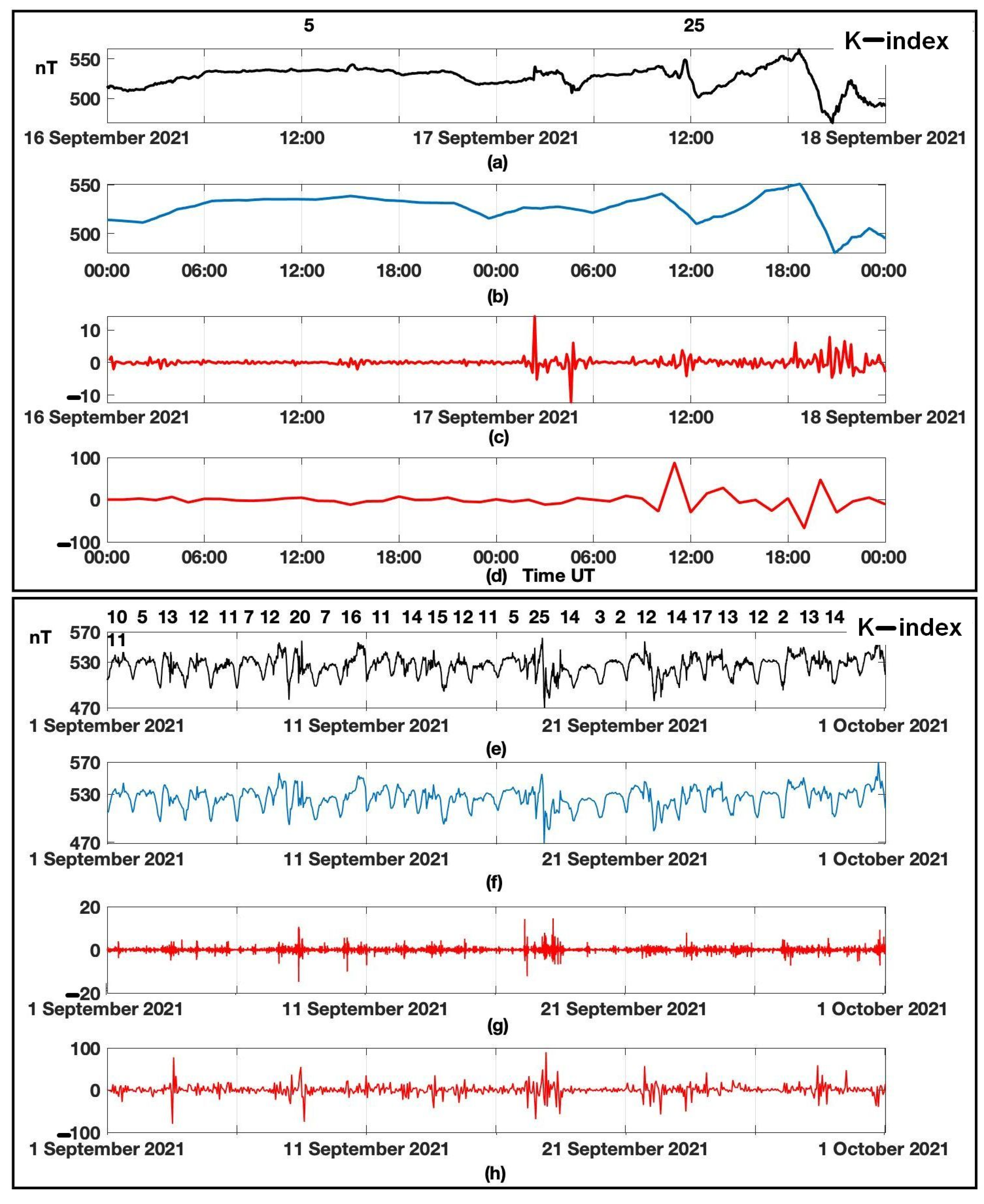
Figure 1 shows the results of the MSA application to the one-minute magnetic data of the Paratunka observatory. The upper panel (Figure 1a–d) shows the results for 16 September 2021 (diurnal K-index = 5) and for 17 September 2021 (diurnal K-index = 25). The lower panel (Figure 1e–h) presents the results for the period of 1–30 September 2021. Diurnal values of K-index are indicated in the upper part of the panels. Smoothed components (Figure 1b,f) approximates signal trend and the detailing components (Figure 1c,d) contain short-period variations of different structures and duration. Analysis of the results shows that during calm periods (K-index has low values), MSA smoothed components allow us to obtain an approximation to the field calm variation. During disturbed periods, a significant increase of detailing component coefficients characterizes the field disturbance degree.
The smoothed component describes geomagnetic signal variations during quiet periods. The obtained approximation error depends on the decomposition level the problem arises in determining the decomposition level , which minimizes the error. Sq-curve can be used as a reference function, reflecting quiet geomagnetic field diurnal variation at an observation site [41]. As described above, Sq-curve is a mean smoothed curve of the five «quietest» intervals of the geomagnetic field over a current month. In this case, the approximation error in wavelet space can be determined as
where are the signal smoothed component coefficients at the decomposition level are the Sq-curve smoothed component coefficients at the decomposition level are readings; is the signal component length.
When choosing the decomposition level , one should also take into account the fact that according to (2), during the change from the decomposition level to the decomposition level , a part of the information on the signal turns to the detailing component (see (2)) that increases the losses
where are the reconstructed signal coefficients obtained on the basis of wavelet recovery and using only approximation coefficients; are the initial signal coefficients, is the signal length.
Thus, according to (3) and (4), we have a problem of multicriteria optimization in which the objective functions
are mutually conflicting. In this case, the optimum level can be obtained by the method of constraint change (-constraints):
The value is considered as an admissible level for , were estimated for each station as the dispersion of geomagnetic field variations during «quiet» periods (absence of magnetic storms and substorms).
From the above said we obtain the algorithm to choose the decomposition level :
- We apply the MSA for the initial data estimated for each month of Sq-curves and obtain the representations , , , where ( is the signal length);
- For each decomposition level we carry out the reconstruction and and estimate the error and losses ;
- We determine the decomposition level providing the least error under admissible losses (conditions (5)).
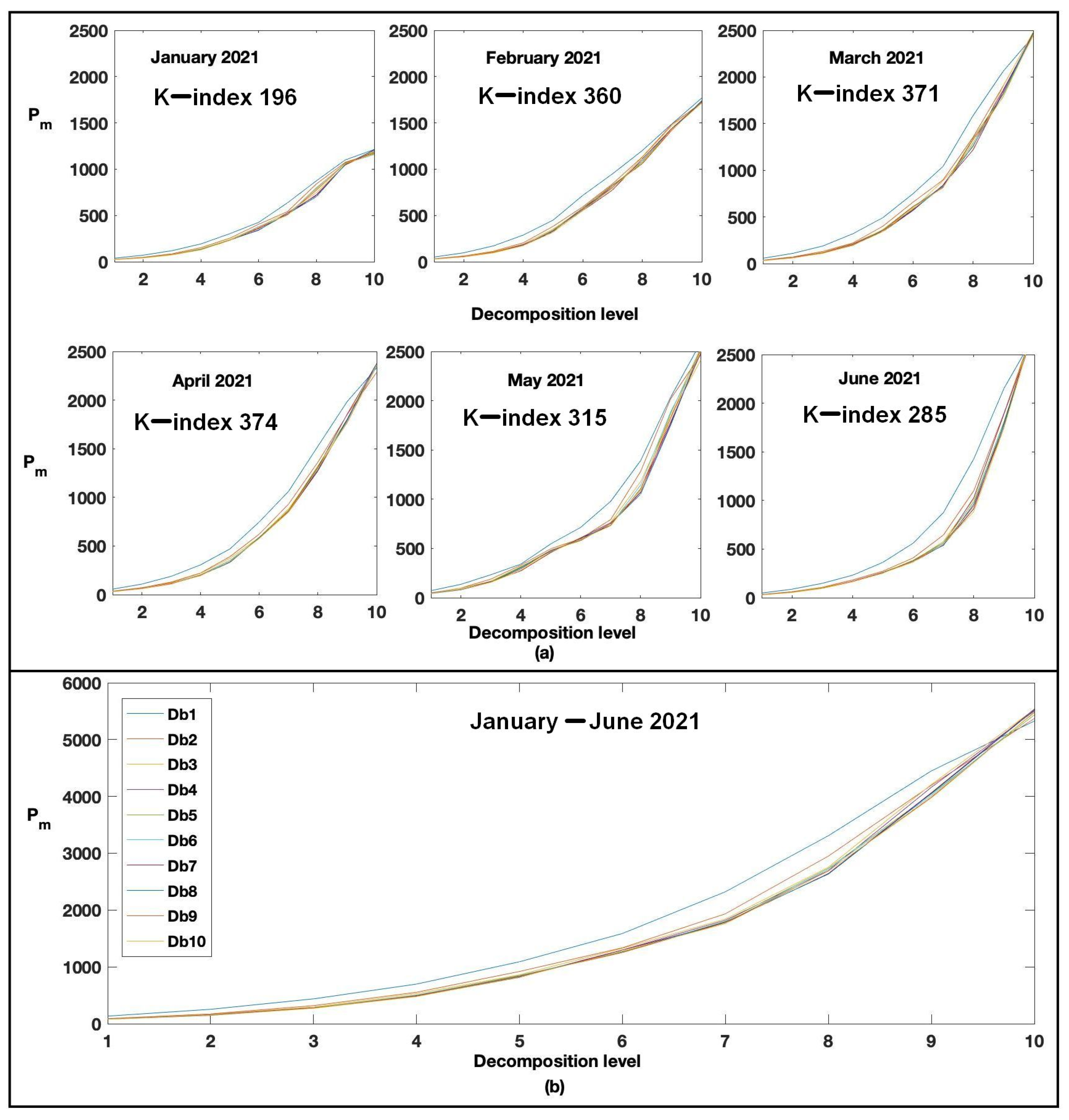
The obtained estimates of and depend on the applied basic wavelet, the choice of which can be based on minimizing the loss function on the set of wavelet basis dictionaries. Figure 2 illustrates the calculation results of the losses for different basic wavelets. Daubechies wavelets of the 1-st–10-th orders, Db1–Db10 were used [30]. The estimates were calculated according to months (for January–June 2021) and for the whole period of the first half of 2021. To analyze geomagnetic activity, Figure 2 presents the K-index summary values for the periods under analysis. The results show close values of (see ratio (4)), including the decomposition 10-th level. A comparison with geomagnetic activity data shows loss increase when the geomagnetic field disturbance degree grows. The result indicates the complicated structure of geomagnetic data, containing features of different forms. Close loss values indicate the possibility of applying different wavelets for geomagnetic data approximation.
To assess the method efficiency, the results were compared with the method for construction of nonlinear approximations in wavelet basis described in the paper [42]. Decompositions into wavelet packages were applied. They allow one to obtain the best signal approximations of finite length by minimizing the concave cost function (entropy) [42].
When considering the dictionary of orthonormal bases
the approximation cost in the basis can be estimated by Shur concave sum [43]
Then the optimal basis minimizing the losses
where is the estimate of the function is determined as
Recursive computation of bases (7), when moving upwards along a wavelet package tree, allows us to obtain an optimal basis, minimizing the cost (6). Construction of an optimal basis is described more in detail in this paper [43].
Estimate results, obtained according to the data of the Paratunka observatory for January 2021 (K-index total value = 196) and for March 2021 (K-index total value = 371), are illustrated in Table 1 and Table 2, respectively. They show that the losses of the optimal basis are significantly less than the losses of the suggested method. However, the errors of the optimal basis determined according to ratio (3) as
significantly exceed the errors of the suggested method, where is the Sq-curve; as long as the Sq-curve, which describes the calm course of geomagnetic field variations, is taken as a reference function for the main condition in method (5) when making estimates and is the one providing the least error . In this case, the decomposition level is determined so that the losses do not exceed the acceptable value (see (5)). The result confirms the efficiency of the suggested method.
Comparison of the results obtained for different basic wavelets (Db1–Db10) shows close values of errors and losses both during low (January 2021, Table 1) and during high (March 2021, Table 2) geomagnetic activity. The results confirm the author’s statement [42] that if a signal contains different structure features localized at different times, it is impossible to construct a basis adapted to all the structures. That also confirms the possibility of application of different wavelets for geomagnetic data approximation.
2.2. Identification of the Model Disturbed Component
Geomagnetic field disturbance degree is the quantity that, according to the paper [41], can be estimated by finding the difference between the highest and the least deviations of signal values from the corresponding values of a quiet diurnal variation. In the proposed model (1), geomagnetic disturbances are described by the component . Following the paper [31] and considering the significant nonstationarity , we shall use the continuous wavelet transform and adaptive threshold functions to identify it.
Then for we obtain the representation:
are the threshold functions determining the respectively weak (of class) and strong (of class) geomagnetic disturbances
, , is the threshold coefficient, , is the wavelet coefficient average calculated in a moving time window of length .
Taking into account the equivalence of the discrete and continuous wavelet transform [29,30], when selecting the wavelet we can use the estimates obtained for discrete decompositions (Table 1 and Table 2, Section 2.1).
The intensity of positive and negative disturbances of the geomagnetic field of each class at the time can be estimated as
The thresholds in (8) are determined by the root-mean-square deviation (), which is estimated dynamically in a moving time window of duration . That provides adaptation of thresholds to signal properties change.
The coefficients of the thresholds (see (8)) can be determined by minimizing the posterior risk [44]. In that case, having posterior data losses can be calculated as
where is the loss function, is the conditional probability of falling within the domain , if the state is the case, are the state indexes (symbol “/” denotes conditional probability). By averaging the conditional risk function over all the states we obtain average risk
where is the prior probability of the state .
For a simple loss function , using posterior probabilities , we obtain the posterior risk
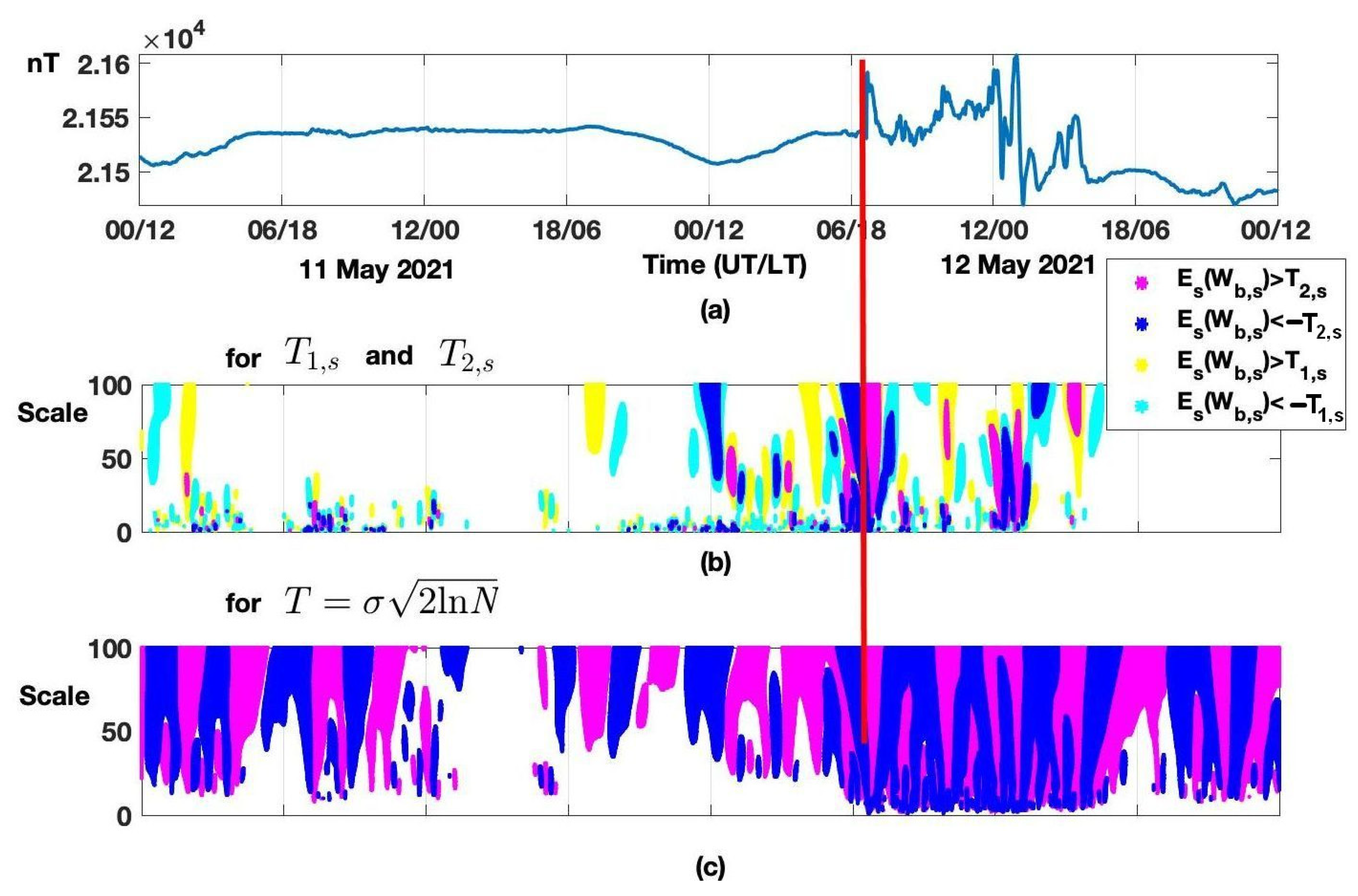
Minimizing the risk , we obtain the best estimates when there is no a priori knowledge on a useful signal and the presence of a high noise level. Figure 3 shows the results of the application of operations (8) to geomagnetic field data of the Paratunka observatory during the magnetic storm on 12 May 2021. The results show that the application of adaptive thresholds (Figure 3b) allows for the detection of weak (threshold ) and strong (threshold ) geomagnetic disturbances before and during a magnetic storm. As a comparison, Figure 3c illustrates the results of the application of the threshold [45]. It was proved in the paper [45] that in white noise case with dispersion , the threshold allows us to obtain the estimates close to optimal ones. The results show that the application of the threshold (Figure 3c) does not allow one to localize the features and to suppress noise in a signal completely. The results confirm the efficiency of the suggested method and agree with the results of the paper [46], in which it was shown that the application of adaptive thresholds allows one to obtain more accurate estimates in the case of data with features of a different structure and a high level of noise. The results also confirm the author’s statement [42] that when signal energy is relatively low noise energy, optimal estimates give too small a threshold and its application does not make it possible to obtain satisfactory results.
3. Calculation of Results and Discussion
In the calculations, we used the magnetic data with the 0.5-s rate (raw and pre-processed) obtained at the Paratunka observatory since 2009 and one-minute data calculated according to INTERMAGNET standards.
The choice of the observatory was determined by the presence of representative data sampling and the detailed description of measurement conditions, such as noise and its sources in raw data, and the magnetologists’ qualification level required for the correct processing of the results of the observations. Information on noise was used to estimate the possibility to apply the method in the mode close to real time. The method application results are shown in Figure 4, Figure 5, Figure 6, Figure 7, Figure 8, Figure 9 and Figure 10.
3.1. Approximation of Geomagnetic Field Quiet Variations
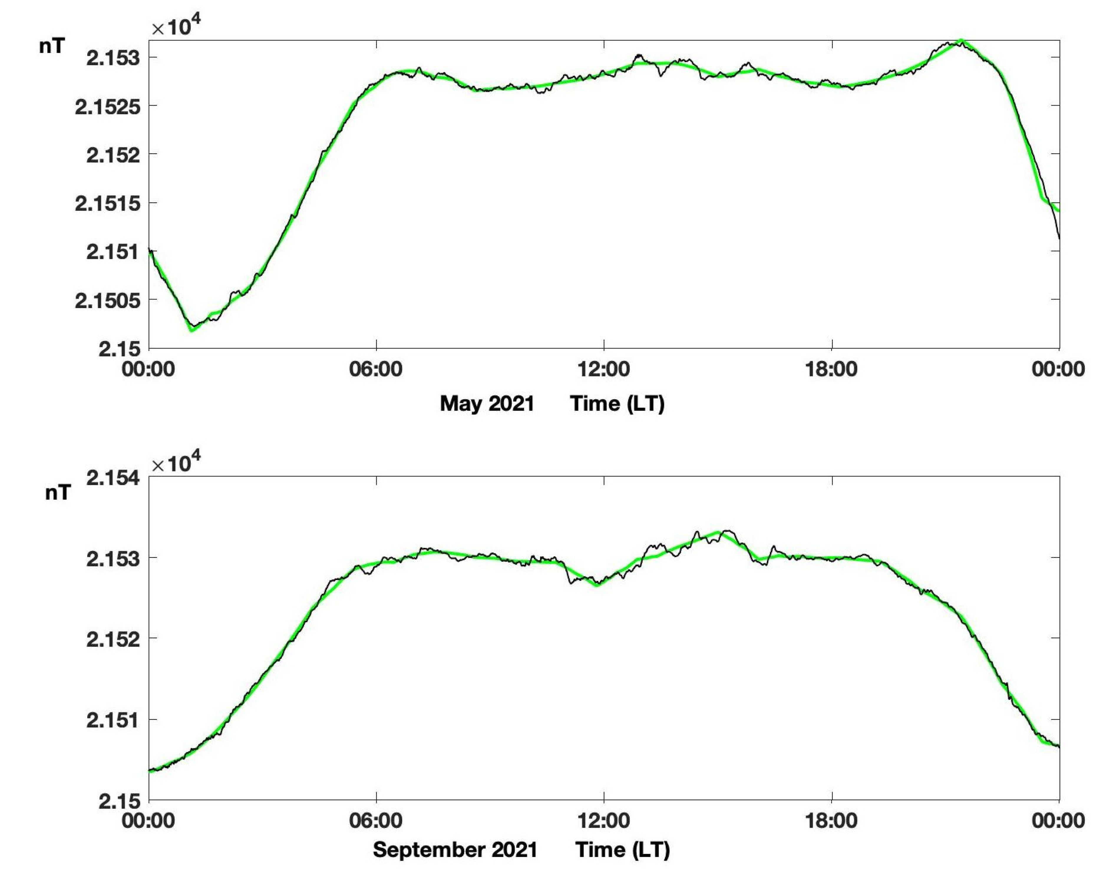
Figure 4 illustrates the Sq-curves for March and September 2021. They were calculated by a traditional technique (black curve at Figure 4) and based on smoothed components of the 6-level decomposition (green curve). The optimum decomposition level is determined with the algorithm described above. The results show that Sq-curves obtained by the proposed method allow us to get a better approximation to the quiet variation, compared with the traditional approach, and confirm the method efficiency.
3.2. Detection of Short-Period Geomagnetic Disturbances, Second-Resolution Data Processing
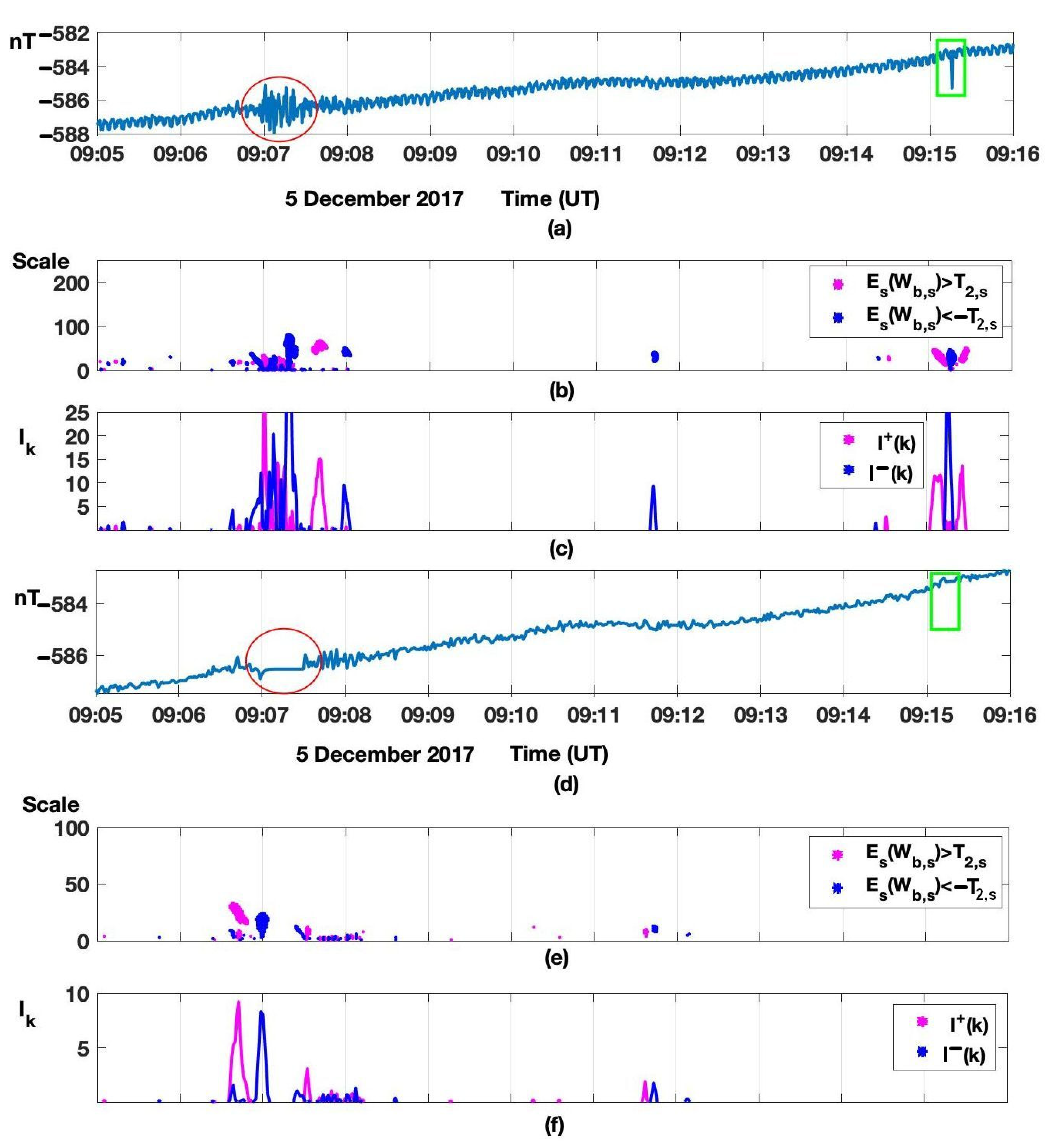
Figure 5, Figure 6 and Figure 7 show the processing results for the raw second data and the data used during the preparation of INTERMAGNET preliminary minute values. The data were obtained on 5 December 2017, by a fluxgate magnetometer FGE-DTU [47], installed at the Paratunka observatory within the scientific cooperation between IKIR FEB RAS and the Deutsches GeoForschungsZentrum GFZ (Helmholtz-Zentrum Potsdam). The magnetometer sensitivity is up to 0.01 nT and the measurement frequency is 2 Hz. A suspended system of sensors is used in the magnetometer. It automatically aligns the Z-axis to a vertical position; however, it causes sensitivity to mechanic impacts on the magnetometer basis, for example, during seismic wave passing or severe shocks near an installation place. There is some noise (oscillations) in the interval under consideration in the records. It is caused by the earthquake that occurred at 09:06:04 UT at a depth of 40 km and about 170 km away from the observatory. The earthquake class was Ks = 10.6 (Figure 5, Figure 6 and Figure 7, red oval). Noise effects from earthquakes can reach one-hundreds of nT depending on distance, depth, and magnitude. A known and quite frequent problem of the observatories carrying out different kinds of measurements is interference from radio devices, for example, from ionosondes and radars located near magnetometers. At the Paratunka observatory, short packages of noise are observed every 15 minutes in records of FGE-DTU magnetometer. They occur during the ionosphere vertical sounding by automatic ionosonde Parus (Figure 5, Figure 6 and Figure 7, green box). One more common issue is the mutual influence of closely located magnetometers. For example, magnetometers with coil systems, such as dIdD GSM-19FD or POS-4, create additional magnetic fields around a sensor during current overlapping in coils. Additional fields also occur around the connecting cables and proton magnetometer sensors during the polarization process. An example of the latest effect is illustrated in Figure 5, Figure 6 and Figure 7, panel (a) Overhauser magnetometer GSM-90 generates noise in FGE-DTU measurements in the form of a meander with the period of 5 s and amplitude of 0.5 nT and more. A detailed description of the noise mentioned above is given in the paper [48].
Standard processing of FGE-DTU records by a magnetologist at the Paratunka observatory includes some operations. The effect from GSM-90 with 5-s cycle is removed by selecting the FGE data out of the time interval when GSM-90 polarization occurs. In this case, the uniform set of values with the frequency of 2 Hz is uniformly gaped with a frequency decrease to 0.4–0.5 Hz. The noise from the ionosonde is regular and occurs at known times, thus, it is removed automatically when a magnetologist has determined sounding parameters and noise duration during sounding. Irregular noise, for example, from earthquakes, is visually identified by a magnetologist from the raw curves. Noised intervals are marked and are not used in further processing [49].
Our algorithms applied in the analysis need the series with uniformly distributed data without gaps. Thus, the gaps were preliminarily filled on a uniform greed by the nearest neighbor method.
Figure 5 shows magnetic field D-component variations (Figure 5a presents raw data, Figure 5d presents data processed by a magnetologist) and the results of method application (Figure 5b,c,e,f; (8), (9) operations were used). The analysis shows evident noise generated by an earthquake and the ionosonde (Figure 5a, red oval and green box). Comparison of the method results obtained for the raw data (Figure 5b,c) and preliminarily processed data (Figure 5e,f), shows a significant impact of noise on the processing results at the times of its occurrences. Evidently, the anomalies occurred as a result of high noise amplitude. We should note that noise manifestation in the method results is observed only near the signal containing noise, compared, for example, to Fourier methods. The result is provided by wavelet finiteness [29,30].
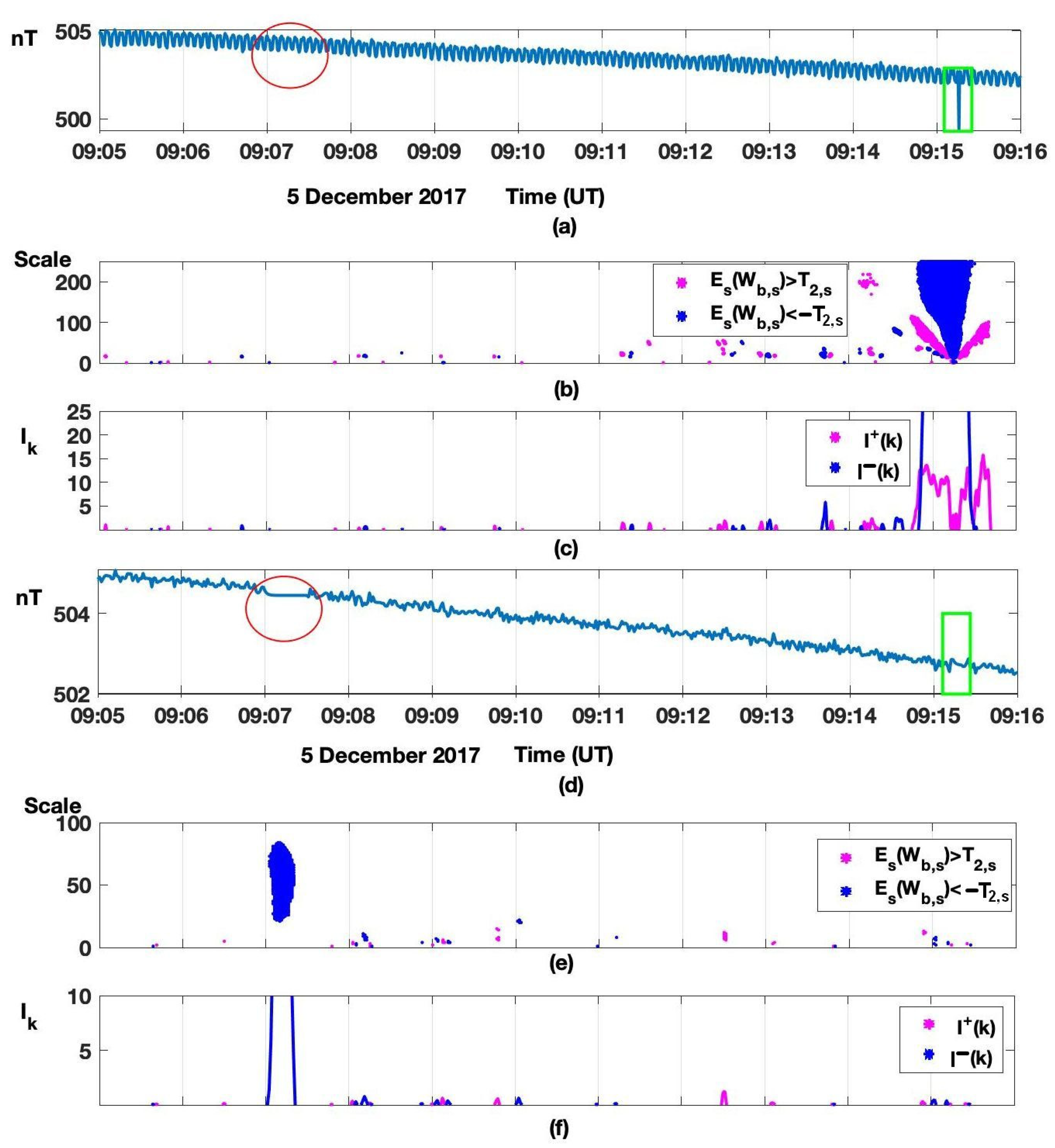
Figure 6 shows the vertical Z-component variations (Figure 6a presents initial data, Figure 6d presents pre-processed data) and the results of method application (Figure 6b,c,e,f). We can see on the graphs that short (duration is several seconds) noise impact from the ionosonde (Figure 6a, green box) was removed after preliminary processing (Figure 6e,f). Noise from the earthquake at 09:07 UT does not have a visible reflection in the time series (Figure 6a, red oval). However, after the preliminary processing (Figure 6d), a false anomaly appeared due to the removing of part of the data (Figure 6e,f), the correction for the nonorthogonality of H-, D-, and Z-sensors is taken into account in Z-variations. Therefore, data removal in variations H and D causes the gap in the Z record. We should note that the problem of correct and effective filling of the gaps in geomagnetic data is topical, does not have indisputably recommended methods at the present time, and is often solved individually for each case.
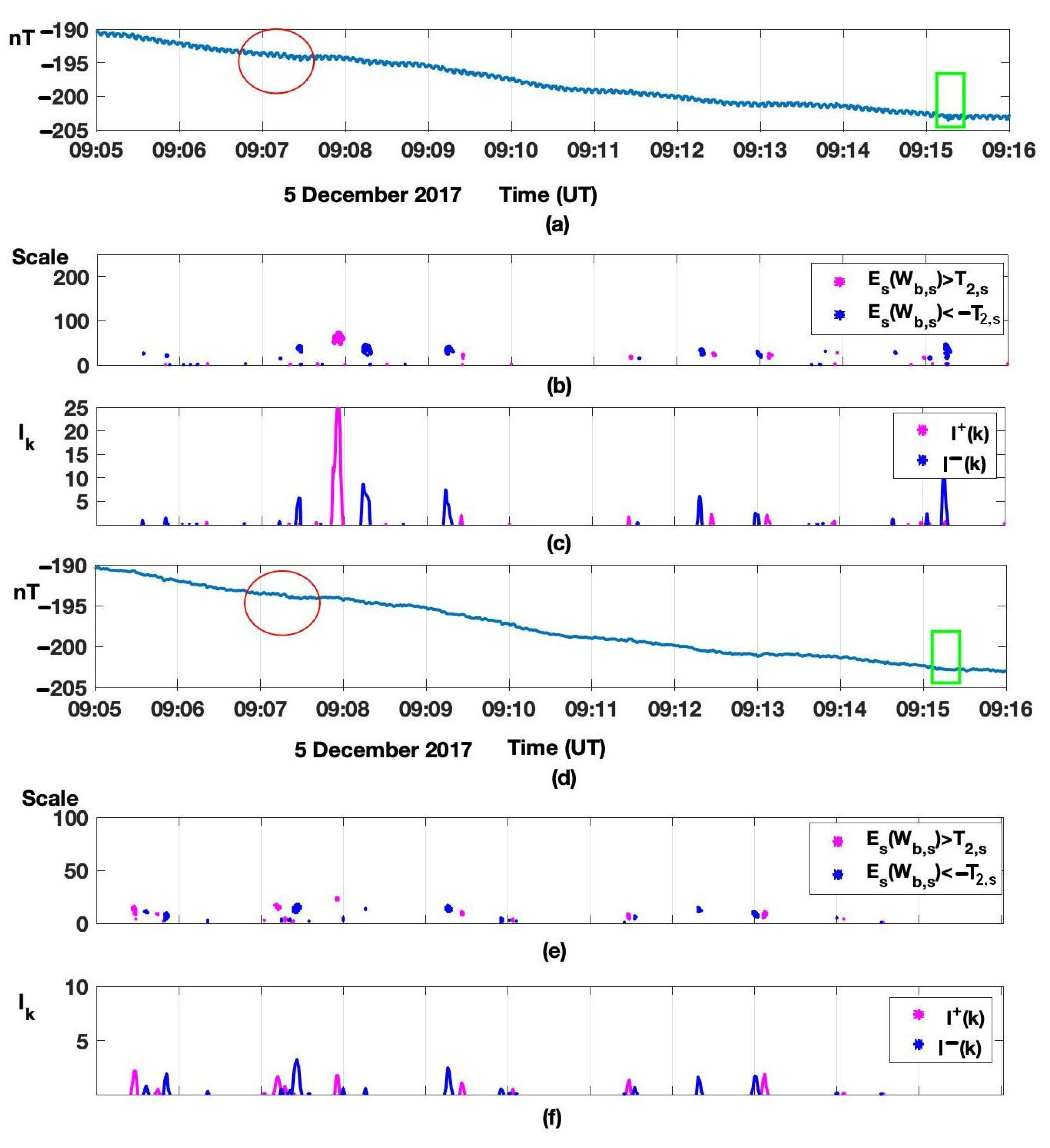
Analysis of horizontal component H variations (Figure 7) shows that the considered noise has small amplitude and does not significantly impact method results. Regular interference in the shape of a meander also does not affect the processing results. That allows us to apply the suggested method to analyze geomagnetic data (H-components) in online mode and to obtain results with admissible accuracy in case of short low-amplitude noise. Sudden changes caused by external impact (ionosonde or earthquake effects) of large amplitude should be identified and removed by a magnetologist during the preliminary analysis and processing of raw data, or they should be separately marked in processing results. Estimates showed that if noise amplitude is more than 1–3 nT (depending on regular oscillations caused, for example, by GSM-90 interference), they should be removed to obtain reliable results. Filling long gaps in geomagnetic data, especially when choosing inadequate filling methods, causes significant distortions of natural variation changes and the appearance of false anomalies in results.
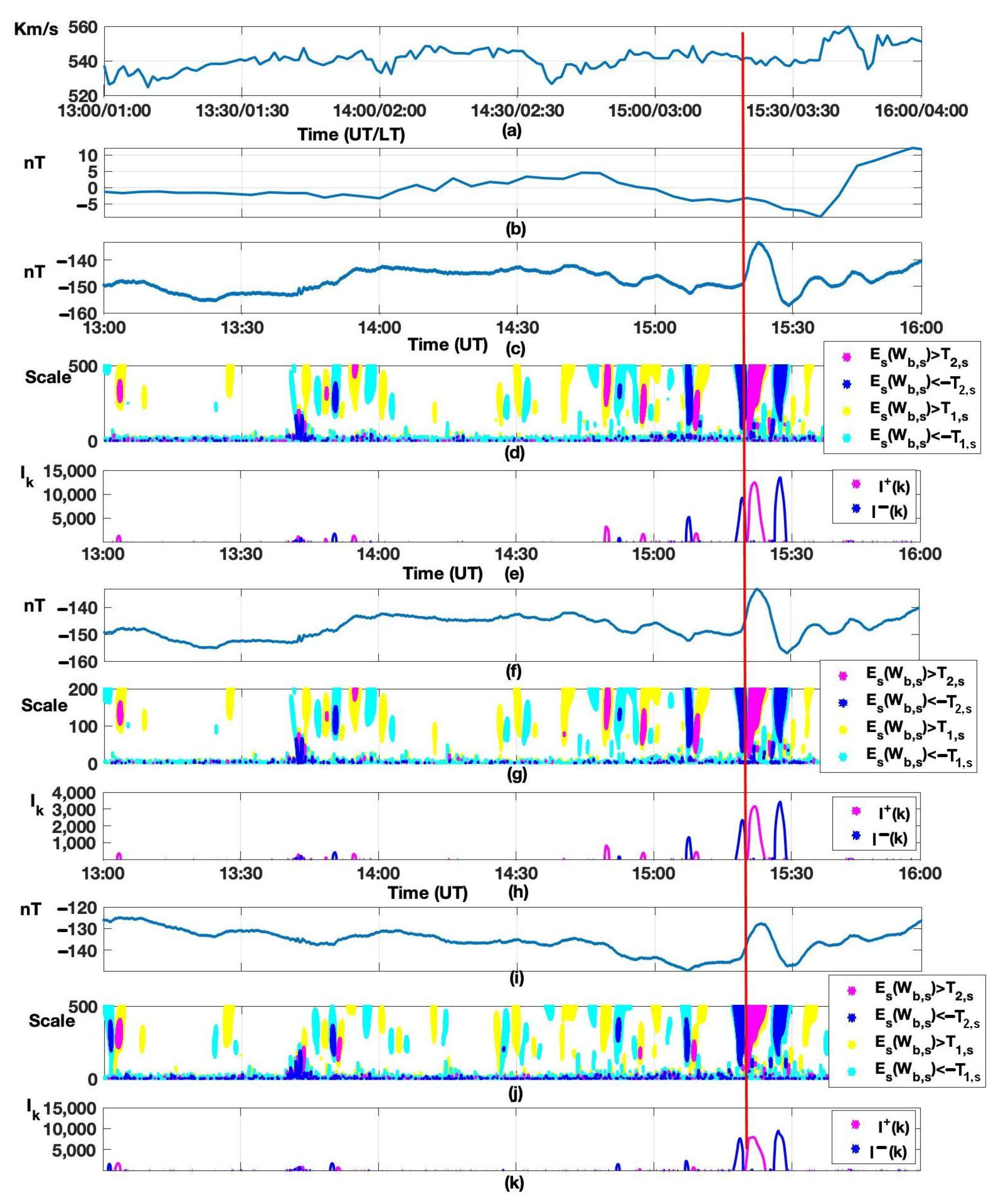
Figure 8 illustrates the results of method application (operations (8) and (9)) for the beginning of a magnetic storm on 21 April 2017. In operation (8), coefficient values (threshold ) and (threshold ) were used. The moving time window length corresponded to one hour and was counts for the initial data and for the preliminarily processed data. The Paratunka observatory data processing results are illustrated in Figure 8d,e (initial data) and Figure 8g,h (data preliminarily processed by a magnetologist). For comparison, Figure 8j,k shows the results of the processing of a raw dataset of the Magadan observatory of IKIR FEB RAS (IAGA code is MGD, 60.05 N, 150.72 E). These data were not preliminarily processed since noise amplitude did not exceed 0.5 nT. To estimate the state in the near-Earth space, the upper part of Figure 8 represents solar wind speed (SWS) (Figure 8a) and interplanetary magnetic field vertical component IMF Bz (Figure 8b).
According to the resource [50] data, SWS increased from 360 to 500 km/s in the middle of the day on 20 April, IMF Bz fluctuations grew up to Bz = ±12 nT. The magnetic storm began on 21 April at 15:19 UT (red vertical line). The analysis of method results (Figure 8d,e,j,h,j,k) shows short-period geomagnetic disturbances at the Paratunka and Magadan observatories before the event. Disturbances increased as the storm beginning was approaching. We can also note the short-time insignificant increase of geomagnetic activity from 13:45 to 14:00 UT at the times of SWS growth (Figure 8a) and insignificant increase of southward IMF Bz fluctuations (Figure 8b). At the time of the storm beginning, disturbance intensity increased significantly. A comparison of the results for the data from different observatories shows clear common dynamics of the process. Still, at the Magadan observatory, the disturbances have the highest amplitude associated with the site location near auroral latitudes. A comparison of the results for initial (Figure 8d,e) and preliminary processed data (Figure 8g,h) shows that noise does not affect the method results significantly and confirms its efficiency.
3.3. Detection of Short-Period Geomagnetic Disturbances, Minute-Resolution Data Processing
Minute-resolution data were obtained using the method defined by INTERMAGNET standards ([51], Section 2.4). Filtering, with Gaussian weight coefficients, was applied to the second data on the interval of −45 … +45 s. Minute value was centered at the beginning of a minute. When some second values were missing, weight renormalization was carried out.
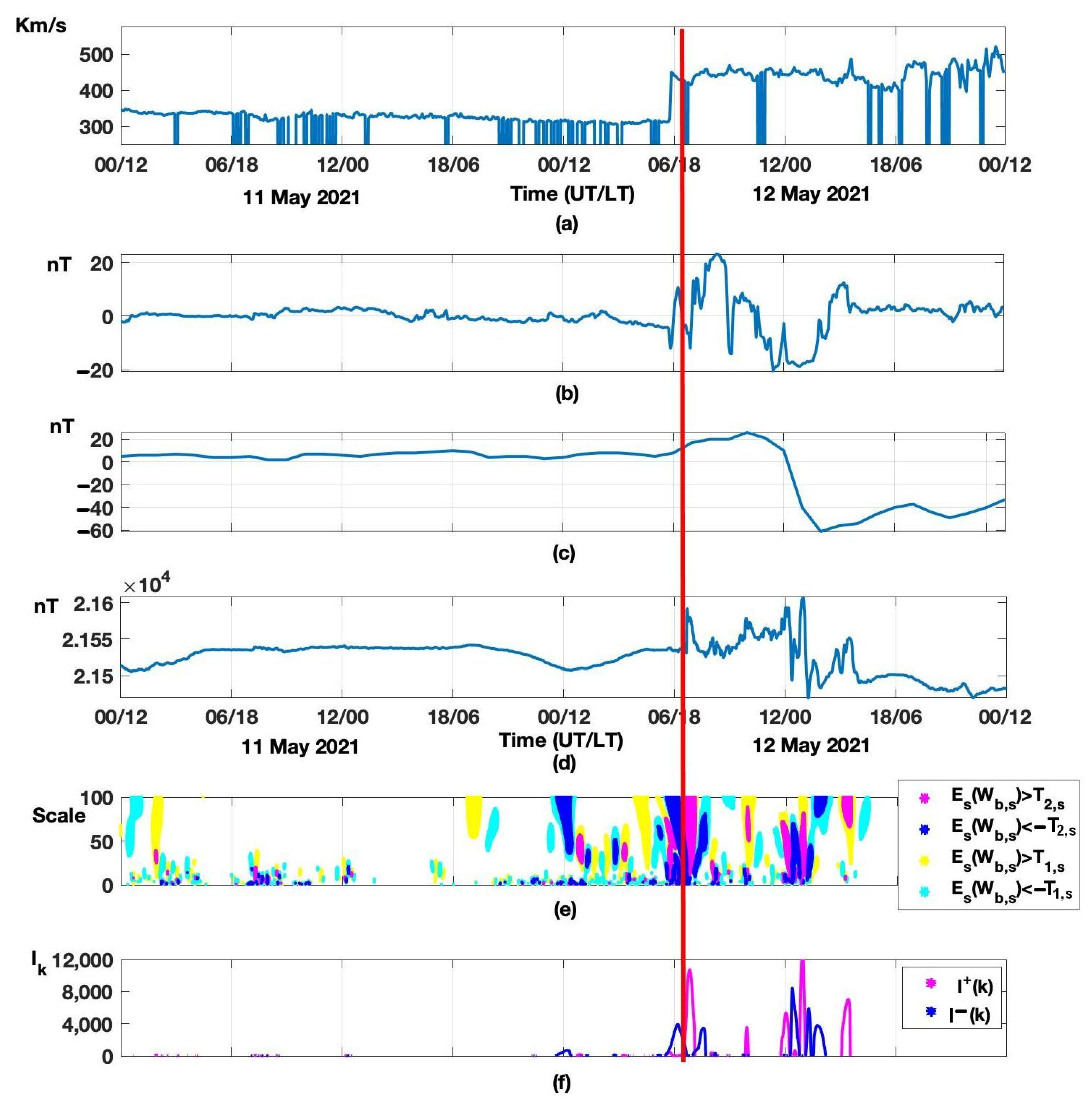
Figure 9 and Figure 10 show the results of the method applied for a moderate magnetic storm on 12 May 2021. To estimate the near-Earth space state, the upper panels of Figure 9 show SWS (Figure 9a), IMF Bz (Figure 9b), and geomagnetic activity Dst-index (Figure 9c). According to the resource [50] SWS was about 300 km/s on 11 May, IMF Bz fluctuations were within ±2 nT. The application of operations (8) and (9) to the PET minute data are illustrated in Figure 9e,f. In operation (8) threshold coefficient was used (positive and negative disturbances exceeding the threshold are illustrated in Figure 9 by pink and by blue, respectively). Based on the ratio (8), application of the coefficient allows one on each scale to detect wavelet coefficient fluctuations exceeding in amplitude the 2.5 RMSD from their characteristic values () within the time window under analysis (window length counts, corresponding to 12 hours, was used). To detect weaker geomagnetic disturbances, threshold coefficient was used (positive and negative disturbances exceeding the threshold are illustrated in Figure 9 by yellow and light blue, respectively). We should note that the times of weak geomagnetic disturbance occurrences before the event correlate with the corresponding small IMF Bz fluctuations times. Moreover, a clear increase in disturbance intensity is observed as the magnetic storm beginning is approaching. A similar character of pre-storm short-period geomagnetic disturbances, according to the meridional station network and auroral zone stations, was mentioned in the papers [31,32]. Strong magnetic storms on 7 January and 17 March 2015 [32] and weak magnetic storms on 9 July and 27 September 2017 were under analysis [31].
Based on space weather data [50], an inhomogeneous accelerated flux from a coronal hole and coronal mass ejection (CME from 9 May) arrived at 05:49 UT on 12 May. During that period, SWS suddenly increased (Figure 9a), and IMF BZ fluctuations increased to Bz = ±20 nT (Figure 9b). The time of the storm’s sudden commencement is evident on the magnetic field H-component graph (Figure 9d, red vertical line). The results of data processing (Figure 9e,f) show that geomagnetic disturbances exceeding the threshold occurred at the Paratunka observatory from 00:00 UT (12:00 LT) to the time of storm beginning on 12 May. Several hours before the storm, during SWS sudden increase (Figure 9a) and IMF Bz southward turn (Figure 9b), disturbance intensity increased significantly and reached (Figure 9f). That is likely to be associated with the beginning of compression region formation.
Strong geomagnetic disturbances were observed during the IMF Bz southward turns and fluctuation intensification during the storm initial phase. IMF Bz northward direction accompanies a geomagnetic activity decrease. During the IMF Bz long southward turn, the storm main phase occurred. It was characterized by a sudden decrease in Dst-index (Figure 9c) and significant increase in H-component fluctuations (Figure 9d). We should note that the Paratunka observatory was in the night sector (00:00–02:00 LT) during that period. Based on the processing data, the intensity reached the values near the H-component minimum values. That is likely to be associated with ring current effects and intensification of the magnetosphere tail currents. The results agree well with those represented in the papers [52,53].
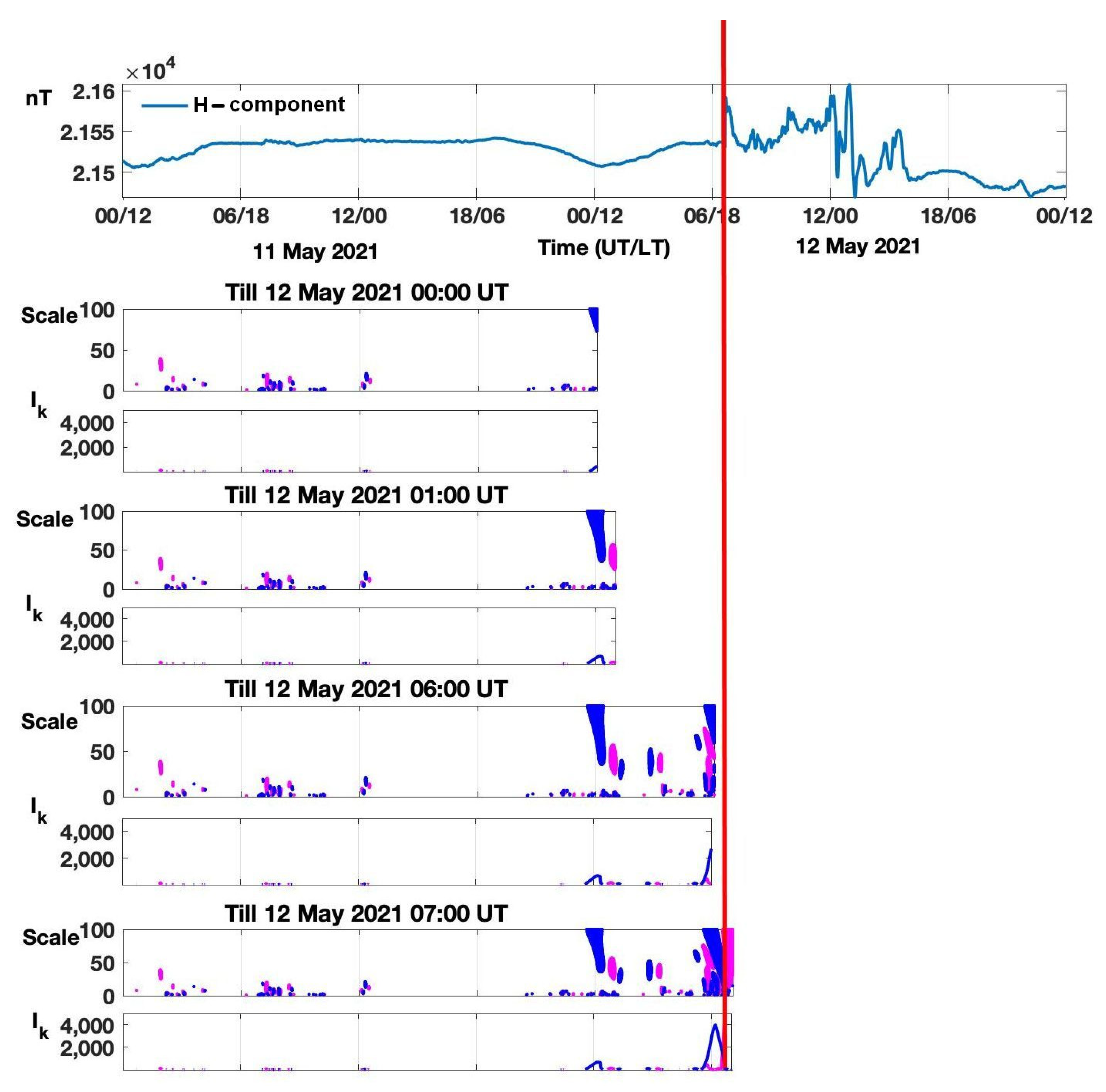
Figure 10 shows the processing results for the Paratunka observatory data for the same period, but the processing was sequential up to the storm beginning. The obtained results of processing (Figure 10, operations (8), (9) applied) agree with the results illustrated in Figure 9. That confirms the method efficiency and shows the possibilities of its application for fast detection of short-period geomagnetic disturbances preceding a magnetic storm beginning.
4. Conclusions
Investigation results confirmed the proposed method’s efficiency for detecting short-period geomagnetic disturbances of differing intensity and duration. Adaptivity of the wavelet model and high time resolution of the suggested approach allow us to investigate sudden small-amplitude variations of the geomagnetic field, which are of interest in space weather. The method makes it possible to process the data of different resolution and, compared to neural networks, does not require periodic rearrangement of algorithm parameters.
Comparison of the proposed wavelet model with the Sq-curve method showed its advantage. The model allows one to obtain a better approximation to geomagnetic field quiet variation than the traditional approach. The method efficiency was also confirmed on the basis of the comparison of its results with the results of application of the optimal threshold suggested in the paper [45].
Comparing the processing results of raw geomagnetic data with the data preliminary processed by a magnetologist confirmed the possibility of applying the method in online mode. In the case of short low-amplitude noise (amplitude is 1–3 nT), the method makes it possible to obtain results with admissible accuracy and can be used to perform data online analysis. The result is important as long as a great and constantly growing volume of recorded geomagnetic data cannot be analyzed manually within a reasonable amount of time. Sudden high amplitude changes caused by external impacts (for example, ionosonde or earthquake effect) can generate false anomalies. In that case, preliminary processing of the data by a magnetologist is required to improve the analysis accuracy. That indicates the necessity to develop automatic detection methods and compensation of noise in geophysical data. One of the possible solutions to the problem was considered in the papers [6,54].
An analysis of the data during disturbed periods confirmed the investigation results [31,32] and showed the possibility of short-period geomagnetic disturbances preceding a geomagnetic storm beginning. Weak short-period increases in geomagnetic activity before storms were described in a number of papers [3,4,5,55]. During the events under consideration, geomagnetic disturbance intensity increased during SWS growth and intensification of southward IMF Bz. As the storm beginning approached, disturbances were intensified. The observed correlation of the detected geomagnetic disturbances with interplanetary environment parameters indicates their external nature and relation with an oncoming magnetic storm.
Summarizing the work results shows the complicated dynamics of the processes in the near-Earth space during increased solar activity and magnetic storms. Investigation of the processes requires the development of methods for data analysis and an extended observation network. The results confirmed the importance of ground observations, which, together with space data, are a valuable and informative tool for space weather monitoring. The investigation also showed the essential role of site observations, which significantly contribute to the investigation of near-Earth space processes and space weather forecast.
Author Contributions
Conceptualization, O.M.; methodology, O.M.; software, Y.P.; formal analysis, O.M. and Y.P.; resources, S.K.; data curation, S.K.; writing—original draft preparation, O.M., Y.P. and S.K.; visualization, O.M., Y.P. and S.K.; project administration, O.M. All authors have read and agreed to the published version of the manuscript.
Funding
The work was carried out according to the Subject AAAA-A21-121011290003-0 «Physical processes in the system of near space and geospheres under solar and lithospheric influences» IKIR FEB RAS.
Institutional Review Board Statement
Not applicable.
Informed Consent Statement
Not applicable.
Data Availability Statement
Not applicable.
Acknowledgments
The authors are grateful to the IKIR FEB RAS that support the magnetic observatories Paratunka and Magadan and international network INTERMAGNET (https://intermagnet.github.io (accessed on 17 December 2021)); Coordinated Data Analysis Web (CDAWeb) (https://cdaweb.gsfc.nasa.gov/index.html/ (accessed on 17 December 2021)); GFZ German Research Centre for Geosciences (https://www.gfz-potsdam.de/en/kp-index/ (accessed on 17 December 2021)); Institute of Applied Geophysics (http://ipg.geospace.ru/ (accessed on 17 December 2021)); World Data Center for Geomagnetism, Kyoto (http://wdc.kugi.kyoto-u.ac.jp/dstae/index.html (accessed on 17 December 2021)); Kakioka Magnetic Observatory, Japan Meteorological Agency (http://kakioka-jma.go.jp/obsdata/dataviewer/en (accessed on 17 December 2021)) the data of which were used in the work.
Conflicts of Interest
The authors declare no conflict of interest.
References
- International Real-Time Magnetic Observatory Network. Available online: https://intermagnet.github.io (accessed on 17 December 2021).
- Di Mauro, D.; Regi, M.; Lepidi, S.; Del Corpo, A.; Dominici, G.; Bagiacchi, P.; Benedetti, G.; Cafarella, L. Geomagnetic Activity at Lampedusa Island: Characterization and Comparison with the Other Italian Observatories, Also in Response to Space Weather Events. Remote Sens. 2021, 13, 3111. [Google Scholar] [CrossRef]
- Bailey, R.L.; Leonhardt, R. Automated Detection of Geomagnetic Storms with Heightened Risk of GIC. Earth Planets Space 2016, 68, 99. [Google Scholar] [CrossRef]
- Hafez, A.G.; Ghamry, E.; Yayama, H.; Yumoto, K. Wavelet Spectral Analysis Technique for Automatic Detection of Geomagnetic Sudden Commencements. IEEE Trans. Geosci. Remote Sens. 2012, 50, 4503–4512. [Google Scholar] [CrossRef]
- Soloviev, A.; Agayan, S.; Bogoutdinov, S. Estimation of Geomagnetic Activity Using Measure of Anomalousness. Ann. Geophys. 2017, 59, 3. [Google Scholar] [CrossRef]
- Bogoutdinov, S.R.; Gvishiani, A.D.; Agayan, S.M.; Solovyev, A.A.; Kin, E. Recognition of Disturbances with Specified Morphology in Time Series. Part 1: Spikes on Magnetograms of the Worldwide INTERMAGNET Network. Izv. Phys. Solid Earth 2010, 46, 1004–1016. [Google Scholar] [CrossRef]
- Wahiduzzaman, M.; Yeasmin, A.; Luo, J.-J.; Ali, M.A.; Bilal, M.; Qiu, Z. Statistical Approach to Observe the Atmospheric Density Variations Using Swarm Satellite Data. Atmosphere 2020, 11, 897. [Google Scholar] [CrossRef]
- Fayemi, O.; Di, Q.; Zhen, Q.; Liang, P. Demodulation of EM Telemetry Data Using Fuzzy Wavelet Neural Network with Logistic Response. Appl. Sci. 2021, 11, 10877. [Google Scholar] [CrossRef]
- Zhou, R.; Han, J.; Guo, Z.; Li, T. De-Noising of Magnetotelluric Signals by Discrete Wavelet Transform and SVD Decomposition. Remote Sens. 2021, 13, 4932. [Google Scholar] [CrossRef]
- Singh, A.K.; Bhargawa, A.; Siingh, D.; Singh, R.P. Physics of Space Weather Phenomena: A Review. Geosciences 2021, 11, 286. [Google Scholar] [CrossRef]
- Despirak, I.V.; Kleimenova, N.G.; Gromova, L.I.; Gromov, S.V.; Malysheva, L.M. Supersubstorms during Storms of 7–8 September 2017. Geomagn. Aeron. 2020, 60, 292–300. [Google Scholar] [CrossRef]
- Gogatishvili, I.M. Geomagnetic precursors of intense earthquakes in the spectrum of geomagnetic pulsations with frequencies of 1–0.02 Hz. Geomagn. Aeron. 1984, 24, 697–700. [Google Scholar]
- Alabdulgader, A.; McCraty, R.; Atkinson, M.; Dobyns, Y.; Vainoras, A.; Ragulskis, M.; Stolc, V. Long-Term Study of Heart Rate Variability Responses to Changes in the Solar and Geomagnetic Environment. Sci. Rep. 2018, 8, 2663. [Google Scholar] [CrossRef] [Green Version]
- Hanzelka, M.; Dan, J.; Fiala, P.; Dohnal, P. Human Psychophysiology Is Influenced by Low-Level Magnetic Fields: Solar Activity as the Cause. Atmosphere 2021, 12, 1600. [Google Scholar] [CrossRef]
- Zenchenko, T.A.; Breus, T.K. The Possible Effect of Space Weather Factors on Various Physiological Systems of the Human Organism. Atmosphere 2021, 12, 346. [Google Scholar] [CrossRef]
- Stupishina, O.M.; Golovina, E.G.; Noskov, S.N.; Eremin, G.B.; Gorbanev, S.A. The Space and Terrestrial Weather Variations as Possible Factors for Ischemia Events in Saint Petersburg. Atmosphere 2022, 13, 8. [Google Scholar] [CrossRef]
- Zawawi, A.A.; Ab Aziz, N.F.; Ab Kadir, M.Z.A.; Hashim, H.; Mohammed, Z. Evaluation of Geomagnetic Induced Current on 275 kV Power Transformer for a Reliable and Sustainable Power System Operation in Malaysia. Sustainability 2020, 12, 9225. [Google Scholar] [CrossRef]
- Gil, A.; Modzelewska, R.; Moskwa, S.; Siluszyk, A.; Siluszyk, M.; Wawrzynczak, A.; Pozoga, M.; Domijanski, S. Transmission Lines in Poland and Space Weather Effects. Energies 2020, 13, 2359. [Google Scholar] [CrossRef]
- Joo, B.-S.; Woo, J.-W.; Lee, J.-H.; Jeong, I.; Ha, J.; Lee, S.-H.; Kim, S. Assessment of the Impact of Geomagnetic Disturbances on Korean Electric Power Systems. Energies 2018, 11, 1920. [Google Scholar] [CrossRef] [Green Version]
- Kangas, J.; Guglielmi, A.; Pokhotelov, O. Morphology and Physics of Short-Period Magnetic Pulsations. Space Sci. Rev. 1998, 83, 435–512. [Google Scholar] [CrossRef]
- Ghamry, E.; Marchetti, D.; Yoshikawa, A.; Uozumi, T.; De Santis, A.; Perrone, L.; Shen, X.; Fathy, A. The First Pi2 Pulsation Observed by China Seismo-Electromagnetic Satellite. Remote Sens. 2020, 12, 2300. [Google Scholar] [CrossRef]
- Agayan, S.; Bogoutdinov, S.; Krasnoperov, R.; Sidorov, R. A Multiscale Approach to Geomagnetic Storm Morphology Analysis Based on DMA Activity Measures. Appl. Sci. 2021, 11, 12120. [Google Scholar] [CrossRef]
- Chinkin, V.E.; Soloviev, A.A.; Pilipenko, V.A.; Engebretson, M.J.; Sakharov, Y.A. Determination of Vortex Current Structure in the High-Latitude Ionosphere with Associated GIC Bursts from Ground Magnetic Data. J. Atmos. Sol. Terr. Phys. 2021, 212, 105514. [Google Scholar] [CrossRef]
- Zelinsky, N.R.; Kleimenova, N.G.; Gromova, L.I. Applying the New Method of Time-Frequency Transforms to the Analysis of the Characteristics of Geomagnetic Pc5 Pulsations. Geomagn. Aeron. 2017, 57, 559–565. [Google Scholar] [CrossRef]
- Agayan, S.; Bogoutdinov, S.; Soloviev, A.; Sidorov, R. The Study of Time Series Using the DMA Methods and Geophysical Applications. Data Sci. J. 2016, 15, 16. [Google Scholar] [CrossRef] [Green Version]
- Rabie, E.; Hafez, A.G.; Saad, O.M.; El-Sayed, A.-H.M.; Abdelrahman, K.; Al-Otaibi, N. Geomagnetic Micro-Pulsation Automatic Detection via Deep Leaning Approach Guided with Discrete Wavelet Transform. J. King Saud Univ. Sci. 2021, 33, 101263. [Google Scholar] [CrossRef]
- Gruet, M.A.; Chandorkar, M.; Sicard, A.; Camporeale, E. Multiple-Hour-Ahead Forecast of the Dst Index Using a Combination of Long Short-Term Memory Neural Network and Gaussian Process. Space Weather 2018, 16, 1882–1896. [Google Scholar] [CrossRef] [Green Version]
- Fu, H.; Zheng, Y.; Ye, Y.; Feng, X.; Liu, C.; Ma, H. Joint Geoeffectiveness and Arrival Time Prediction of CMEs by a Unified Deep Learning Framework. Remote Sens. 2021, 13, 1738. [Google Scholar] [CrossRef]
- Chui, C.K. An Introduction to Wavelets; Wavelet Analysis and Its Applications; Academic Press: Boston, MA, USA, 1992; ISBN 978-0-12-174584-4. [Google Scholar]
- Daubechies, I. Ten Lectures on Wavelets; CBMS-NSF Regional Conference Series in Applied Mathematics 61; Society for Industrial and Applied Mathematics: Philadelphia, PA, USA, 1992; ISBN 978-0-89871-274-2. [Google Scholar]
- Mandrikova, O.V.; Rodomanskaya, A.I.; Mandrikova, B.S. Application of the New Wavelet-Decomposition Method for the Analysis of Geomagnetic Data and Cosmic Ray Variations. Geomagn. Aeron. 2021, 61, 492–507. [Google Scholar] [CrossRef]
- Mandrikova, O.V.; Solovyev, I.S.; Khomutov, S.Y.; Geppener, V.V.; Klionskiy, D.M.; Bogachev, M.I. Multiscale Variation Model and Activity Level Estimation Algorithm of the Earth’s Magnetic Field Based on Wavelet Packets. Ann. Geophys. 2018, 36, 1207–1225. [Google Scholar] [CrossRef]
- Mandrikova, O.V.; Stepanenko, A.A. Automated method for calculating the Dst-index based on the wavelet model of geomagnetic field variations. Comput. Opt. 2020, 44, 797–808. [Google Scholar] [CrossRef]
- Nosé, M.; Iyemori, T.; Takeda, M.; Kamei, T.; Milling, D.K.; Orr, D.; Singer, H.J.; Worthington, E.W.; Sumitomo, N. Automated Detection of Pi 2 Pulsations Using Wavelet Analysis: 1. Method and an Application for Substorm Monitoring. Earth Planets Space 1998, 50, 773–783. [Google Scholar] [CrossRef] [Green Version]
- Nosé, M. Automated Detection of Pi 2 Pulsations Using Wavelet Analysis: 2. An Application for Dayside Pi 2 Pulsation Study. Earth Planets Space 1999, 51, 23–32. [Google Scholar] [CrossRef] [Green Version]
- Jach, A.; Kokoszka, P.; Sojka, J.; Zhu, L. Wavelet-Based Index of Magnetic Storm Activity. J. Geophys. Res. 2006, 111, A09215. [Google Scholar] [CrossRef] [Green Version]
- Mandrikova, O.; Fetisova, N.; Polozov, Y. Hybrid Model for Time Series of Complex Structure with ARIMA Components. Mathematics 2021, 9, 1122. [Google Scholar] [CrossRef]
- Xu, Z.; Zhu, L.; Sojka, J.; Kokoszka, P.; Jach, A. An Assessment Study of the Wavelet-Based Index of Magnetic Storm Activity (WISA) and Its Comparison to the Dst Index. J. Atmos. Sol. Terr. Phys. 2008, 70, 1579–1588. [Google Scholar] [CrossRef]
- Sugiura, M. Hourly values of equatorial Dst for the IGY. In Annals of the International Geophysical Year; Pergamon Press: Oxford, UK, 1964; Volume 35, pp. 7–45. [Google Scholar]
- Bartels, J.; Veldkamp, J. International Data on Magnetic Disturbances, Fourth Quarter, 1953. J. Geophys. Res. 1954, 59, 297–302. [Google Scholar] [CrossRef]
- Chapman, S.; Bartels, J. Geomagnetism; Oxford University Press: Oxford, UK, 1940. [Google Scholar]
- Mallat, S.G. A Wavelet Tour of Signal Processing; Academic Press: San Diego, CA, USA, 1999; ISBN 978-0-12-466606-1. [Google Scholar]
- Coifman, R.R.; Wickerhauser, M.V. Entropy-based algorithms for best basis selection. IEEE Trans. Inf. Theory 1992, 38, 713–718. [Google Scholar] [CrossRef] [Green Version]
- Bansal, A.K. Bayesian Parametric Inference; Narosa Publishing House Pvt. Ltd.: New Delhi, India, 2007. [Google Scholar]
- Donoho, D.L.; Johnstone, I.M. Ideal spatial adaptation via wavelet shrinkage. Biometrika 1994, 81, 425–455. [Google Scholar] [CrossRef]
- Mandrikova, O.; Mandrikova, B.; Rodomanskay, A. Method of Constructing a Nonlinear Approximating Scheme of a Complex Signal: Application Pattern Recognition. Mathematics 2021, 9, 737. [Google Scholar] [CrossRef]
- Technical University of Denmark (Space). Available online: https://www.space.dtu.dk/english/Research/Research-Divisions/Geomagnetism-and-Geospace/Ground-based-magnetometry-instrumentation-infrastructure-and-data/3-axis_Fluxgate_Magnetometer_Model_FGM-FGE (accessed on 17 December 2021).
- Khomutov, S.Y.; Mandrikova, O.V.; Budilova, E.A.; Arora, K.; Manjula, L. Noise in Raw Data from Magnetic Observatories. Geosci. Instrum. Method. Data Syst. 2017, 6, 329–343. [Google Scholar] [CrossRef] [Green Version]
- Khomutov, S.Y. Methodological and Software Approaches to Processing of Magnetic Measurements of Observatories of IKIR FEB RAS, Russia. J. Ind. Geophys. Union 2016, 2, 54–61. [Google Scholar]
- Institute of Applied Geophysics. Available online: http://ipg.geospace.ru/ (accessed on 17 December 2021).
- St-Louis, B.; INTERMAGNET Operations Committee; INTERMAGNET Executive Council. INTERMAGNET Technical Reference Manual, Version 5.0.0; INTERMAGNET: Edinburgh, UK, 2020; 146p. [Google Scholar]
- Rastogi, R.G. Magnetic Storm Effects in H and D Components of the Geomagnetic Field at Low and Middle Latitudes. J. Atmos. Sol. Terr. Phys. 2005, 67, 665–675. [Google Scholar] [CrossRef]
- Chiaha, S.O.; Ugonabo, O.J.; Okpala, K.C. A study on the effects of solar wind and interplanetary magnetic field on geo-magnetic H-component during geomagnetic storms. Int. J. Phys. Sci. 2018, 13, 230–234. [Google Scholar] [CrossRef]
- Soloviev, A.A.; Agayan, S.M.; Gvishiani, A.D.; Bogoutdinov, S.R.; Chulliat, A. Recognition of Disturbances with Specified Morphology in Time Series: Part 2. Spikes on 1-s Magnetograms. Izv. Phys. Solid Earth 2012, 48, 395–409. [Google Scholar] [CrossRef]
- Sheiner, O.A.; Fridman, V.M. The Features of Microwave Solar Radiation Observed in the Stage of Formation and Initial Propagation of Geoeffective Coronal Mass Ejections. Radiophys. Quantum Electron. 2012, 54, 655–666. [Google Scholar] [CrossRef]
Figure 1.
Application of MSA to Paratunka observatory data applying the Daubechies 3 wavelet. (a,e) H-component; (b,f) component; (c,g) component; (d,h) component.
Figure 1.
Application of MSA to Paratunka observatory data applying the Daubechies 3 wavelet. (a,e) H-component; (b,f) component; (c,g) component; (d,h) component.

Figure 2.
Results of estimation of losses for different basic wavelets, Paratunka observatory data were used. (a) January–June 2021; (b) first half of 2021.
Figure 2.
Results of estimation of losses for different basic wavelets, Paratunka observatory data were used. (a) January–June 2021; (b) first half of 2021.

Figure 3.
Processing results for geomagnetic data for the period 11–12 May 2021. (a) H-component; (b,c) application of thresholds. The red vertical line is the magnetic storm beginning.
Figure 3.
Processing results for geomagnetic data for the period 11–12 May 2021. (a) H-component; (b,c) application of thresholds. The red vertical line is the magnetic storm beginning.

Figure 4.
Black line is the Sq-curve obtained by the traditional method, green line is the Sq-curve obtained by the components , Paratunka observatory.
Figure 4.
Black line is the Sq-curve obtained by the traditional method, green line is the Sq-curve obtained by the components , Paratunka observatory.

Figure 5.
Processing results for D-component variations on 5 December, 2017. (a) D-component, noisy; (d) D-component, cleared; (b,c,e,f) results of method application.
Figure 5.
Processing results for D-component variations on 5 December, 2017. (a) D-component, noisy; (d) D-component, cleared; (b,c,e,f) results of method application.

Figure 6.
Processing results for Z-component variations on 5 December 2017. (a) Z-component, noisy; (d) Z-component, cleared; (b,c,e,f) results of method application.
Figure 6.
Processing results for Z-component variations on 5 December 2017. (a) Z-component, noisy; (d) Z-component, cleared; (b,c,e,f) results of method application.

Figure 7.
Processing results for H-component variations on 5 December 2017. (a) H-component, noisy; (d) H-component, cleared; (b,c,e,f) results of method application.
Figure 7.
Processing results for H-component variations on 5 December 2017. (a) H-component, noisy; (d) H-component, cleared; (b,c,e,f) results of method application.

Figure 8.
Processing of Paratunka and Magadan observatory geomagnetic data on 21 April 2017 (H-component). (a) SWS; (b) IMF Bz (GSM); (c) H-component PET, noisy; (f) H-component PET, cleared; (i) H-component MGD, noisy; (d,e,g,h,j,k) results of method application. Red vertical line is the magnetic storm beginning.

Figure 9.
Processing results for geomagnetic data for the period 11–12 May 2021. (a) SWS; (b) IMF Bz (GSE); (c) DST; (d) H-component; (e,f) results of method application. The red vertical line is the magnetic storm beginning.
Figure 9.
Processing results for geomagnetic data for the period 11–12 May 2021. (a) SWS; (b) IMF Bz (GSE); (c) DST; (d) H-component; (e,f) results of method application. The red vertical line is the magnetic storm beginning.

Figure 10.
Results of sequential processing of geomagnetic data for the period 11–12 May 2021, before the storm beginning.
Figure 10.
Results of sequential processing of geomagnetic data for the period 11–12 May 2021, before the storm beginning.


Table 1.
Method efficiency estimate results, obtained from the data for January 2021.
| Wavelet | of the Optimal Basis | |||
|---|---|---|---|---|
| Db1 | 396.09 | 165.05 | 21.05 | 74.06 |
| Db2 | 349.63 | 141.32 | 21.37 | 53.99 |
| Db3 | 331.57 | 131.04 | 20.99 | 51.76 |
| Db4 | 330.26 | 130.85 | 21.26 | 50.54 |
| Db5 | 329.77 | 130.82 | 21.31 | 50.80 |
| Db6 | 327.42 | 130.91 | 21.06 | 51.55 |
| Db7 | 326.31 | 130.87 | 21.22 | 51.28 |
| Db8 | 329.35 | 131.02 | 21.32 | 50.06 |
| Db9 | 324.30 | 130.90 | 21.14 | 50.89 |
| Db10 | 324.20 | 130.96 | 21.17 | 51.20 |
Table 2.
Method efficiency estimate results, obtained from the data for March 2021.
| Wavelet | of the Optimal Basis | |||
|---|---|---|---|---|
| Db1 | 495.86 | 185.22 | 21.52 | 126.27 |
| Db2 | 459.81 | 170.22 | 21.34 | 68.39 |
| Db3 | 439.88 | 156.99 | 21.52 | 74.70 |
| Db4 | 438.27 | 155.61 | 21.57 | 63.92 |
| Db5 | 437.79 | 148.49 | 21.39 | 62.56 |
| Db6 | 437.09 | 146.00 | 21.51 | 61.23 |
| Db7 | 436.67 | 142.27 | 21.57 | 53.66 |
| Db8 | 336.82 | 145.82 | 21.41 | 61.57 |
| Db9 | 437.02 | 145.80 | 21.44 | 61.90 |
| Db10 | 436.73 | 140.62 | 21.57 | 52.87 |
Publisher’s Note: MDPI stays neutral with regard to jurisdictional claims in published maps and institutional affiliations. |
© 2022 by the authors. Licensee MDPI, Basel, Switzerland. This article is an open access article distributed under the terms and conditions of the Creative Commons Attribution (CC BY) license (https://creativecommons.org/licenses/by/4.0/).
Share and Cite
MDPI and ACS Style
Mandrikova, O.; Polozov, Y.; Khomutov, S. Wavelet Model of Geomagnetic Field Variations and Its Application to Detect Short-Period Geomagnetic Anomalies. Appl. Sci. 2022, 12, 2072. https://doi.org/10.3390/app12042072
AMA Style
Mandrikova O, Polozov Y, Khomutov S. Wavelet Model of Geomagnetic Field Variations and Its Application to Detect Short-Period Geomagnetic Anomalies. Applied Sciences. 2022; 12(4):2072. https://doi.org/10.3390/app12042072
Chicago/Turabian StyleMandrikova, Oksana, Yuriy Polozov, and Sergey Khomutov. 2022. "Wavelet Model of Geomagnetic Field Variations and Its Application to Detect Short-Period Geomagnetic Anomalies" Applied Sciences 12, no. 4: 2072. https://doi.org/10.3390/app12042072
Note that from the first issue of 2016, this journal uses article numbers instead of page numbers. See further details here.