Article

Active Disturbance Rejection Control Based Sinusoidal Trajectory Tracking for an Upper Limb Robotic Rehabilitation Exoskeleton

1
Department of Instrumentation Engineering, Shri Guru Gobind Singhji Institute of Engineering and Technology, Nanded 431606, India
2
Smart Assistive and Rehabilitative Technology (SMART) Research Group, Department of Electrical and Electronic Engineering, Universiti Teknologi PETRONAS, Bandar Seri Iskandar 32610, Malaysia
3
ImViA, Université de Bourgogne Franche Comté, 12 Rue de La Fonderie, 71200 Le Creusot, France
4
School of Biomedical Engineering, University of Technology Sydney, Ultimo 2007, Australia
*
Author to whom correspondence should be addressed.
Appl. Sci. 2022, 12(3), 1287; https://doi.org/10.3390/app12031287
Submission received: 9 November 2021 / Revised: 22 December 2021 / Accepted: 28 December 2021 / Published: 26 January 2022
(This article belongs to the Special Issue The Present and Future of Robotic Technology in Rehabilitation)

Abstract

:
In this paper, a combined control strategy with extended state observer (ESO) and finite time stable tracking differentiator (FTSTD) has been proposed to perform flexion and extension motion repetitively and accurately in the sagittal plane for shoulder and elbow joints. The proposed controller improves the tracking accuracy, performs state estimation, and actively rejects disturbance. A sinusoidal trajectory as an input has been given to a two-link multiple-input multiple-output (MIMO) upper limb robotic rehabilitation exoskeleton (ULRRE) for a passive rehabilitation purpose. The efficacy of the controller has been tested with the help of performance indices such as integral time square error (ITSE), integral square error (ISE), integral time absolute error (ITAE), and integral of the absolute magnitude of error (IAE). The system model is obtained through the Euler–Lagrangian method, and the controller’s stability is also given. The proposed controller has been simulated for ± 20 % parameter variation with constant external disturbances to test the disturbance rejection ability and robustness against parametric uncertainties. The proposed controller has been compared with already developed ESO-based methods such as active disturbance rejection control (ADRC), nonlinear active disturbance rejection control (NLADRC), and improved active disturbance rejection control (I-ADRC). It has been found that the proposed method increases tracking performance, as evidenced by the above performance indices.

1. Introduction

1.1. Motivation and Background

Conventional rehabilitation activities require the patient to work with a therapist and support personnel to complete the targeted rehabilitative training. These activities require repetitive motions over a long period, which is exhaustive for patients and therapists [1,2]. Additionally, this approach lacks quantitative measurement of patient progress, indicating the necessity for more modern methodologies and new technologies to solve this deficiency. Robotic rehabilitation is a popular and contemporary method that integrates robotics expertise with rehabilitation treatment to facilitate recovery [3,4,5,6]. These robotic devices work on the affected area and assist the patient in achieving the highest level of movement precision possible. Additionally, these devices give comfort and may be used for a specific time based on the therapeutic requirements. The outcomes of therapy are analyzed using a continuous assessment and recorded movements of patients undergoing rehabilitation [7].

1.2. Related Research

Various control structures have been adopted so far to improve the functioning of rehabilitation exoskeletons. One popular method is PID control, which performs well but fails and suffers when disturbance affects the system [8]. The particle swarm optimization (PSO) [9] method acts on disturbance but involves the evaluation of many parameters. A model-based technique such as computed-torque control (CTC) [10,11] needs additional control methods to compensate for modeling uncertainties. The development of rules and inference testing in intelligent control approaches are time-consuming tasks [12]. Sensitivity amplification cannot cope with disturbance and requires exact modeling information [13,14]. A neural network based on radial basis functions (RBF) can handle disturbances but has high computational costs [15]. Robust control methods are cautious and take the worst-case scenarios into account. The sliding mode control (SMC) handles the disturbances but has chattering issues [16].
In a nonlinear multiple-input multiple-output (MIMO) system, obtaining precise model information is complex and time-consuming. To meet this requirement, Han [17] developed the extended-state-observer (ESO)-based control or active disturbance rejection control (ADRC). This approach has been utilized in various disciplines, including motion control [18,19,20,21], flight control [22,23], and process control [24,25,26,27,28,29,30,31,32,33,34]. To achieve disturbance rejection, ESO determines the system state utilizing input–output data [35]. ADRC does not rely heavily on exact model knowledge [36,37]. ADRC is characterized as a model-free controller since it just requires the system order and the estimated value of system parameters [38].
The usefulness of the ADRC technique for tracking trajectories has been evaluated over many upper and lower limb robotic rehabilitation exoskeletons in recent years. A lower limb gait trajectory tracking was recently achieved using LESO [39,40] and proved to be more successful than PID. Several enhancements have recently been made to improve the existing LESO-based architecture of ADRC to track accurate trajectories. Guerrero-Castellanos et al. [41] presented ESO combination with control Lyapunov function (CLF) and Sontag’s formula to track active ankle–foot orthosis motion. Rehabilitation strategies for trajectory tracking, force and impedance control, and biosignals have already been developed [42,43,44,45,46,47]. Trajectory tracking is one of the essential aspects of rehabilitation that can be accurately achieved by better control methods for patient recovery [5,40,48,49,50].

1.3. Purpose, Contribution, and Paper Structure

The purpose of this paper is to provide an ESO-based robust controller for performing accurate rehabilitative motions. For the upper limb system model, the flexion and extension movements are given by a sinusoidal trajectory, which is an input to the exoskeleton. The proposed control method precisely tracks these inputs, improving the repeatability of joint movement and aiding the patient’s recovery during the early phases of rehabilitation. In addition to the fact that patients’ musculoskeletal problems differ and may occur while performing such exercises, which can interfere with tracking and consequently the rehabilitation process, the proposed method actively removes these disturbances while tracking.
A trajectory tracking control for two-link ULRRE has been devised in this work. A finite-time stable tracking differentiator based on the ADRC control law has improved trajectory tracking accuracy. The exoskeleton model is obtained using the Euler–Lagrange method. The two units, LESO and FTSTD, estimate the system’s states and eliminate disturbances as lumped disturbances, including modeling uncertainties and external disturbances. FTSTD generates signals by differentiating the input, resulting in an output that increases gradually rather than abruptly, improving accuracy and decreasing overshoot. The proposed work has been compared with recently developed ESO-based trajectory tracking control strategies such as ADRC, NLADRC, and I-ADRC by performing a simulation study. The proposed method’s efficacy has been evaluated using various performance indices with 20% parameter variation and constant external disturbance. Simulation results indicate an improvement in trajectory tracking accuracy with disturbance rejection and robustness against parameter variation.
The rest of the paper is organized as follows: Section 2 focuses on ULRRE modeling. Section 3 details the ESO-based and FTSTD-based ADRC control strategies. The closed-loop stability is described in Section 4. Simulation results are shown in Section 5. Discussion is given in Section 6. Finally, in Section 7, the conclusion is reached.

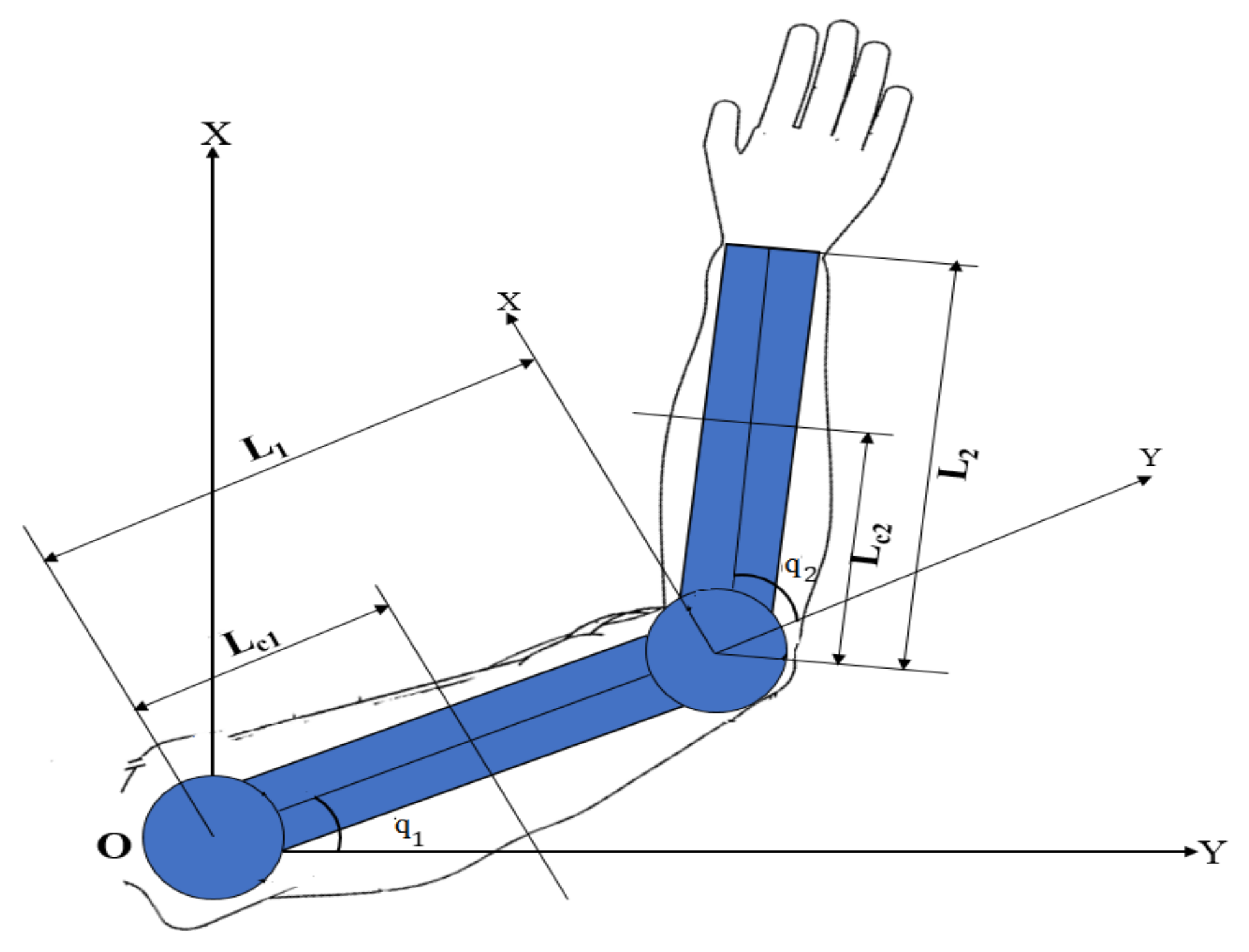
2. Modeling of Upper Limb Robotic Rehabilitation Exoskeleton

Figure 1 shows a two-link ULRRE model. It works in the sagittal plane for flexion and extension movements of shoulder and elbow joints. The electric motors provide these movements. The parameters of ULRRE for both joints are displayed in Figure 1. The lengths of connecting segments from the exoskeleton to the center of masses are L c 1 and L c 2 . The lengths of two links are L 1 and L 2 . The angular positions of the two links are q 1 and q 2 . The model is obtained from [51] and parameters values are shown in Table 1.
The equation of motion was obtained using the Euler–Lagrange method and is presented in Equation (1) as
J ( q ) q . . + C ( q , q . ) q . + G ( q ) + D = T
Table 2 describes the Equation (1).
Properties of dynamic model in Equation (1) are as follows:
  • Matrix J ( q ) is symmetric and positive definite.
  • Matrix J . ( q . ) 2 C ( q , q . ) is a skew-symmetric if ε R n , ε T ( J . ( q . ) 2 C ( q , q . ) ) ε = 0 .
  • There are finite scalars ζ i > 0 , i = 1 , . . . . . , 4 , for which J ( q ) ζ 1 , C ( q , q . ) ζ 2 , G ( q ) ζ 3 and D ζ 4 , that suggest all elements of model are bounded.
The equations of matrices are given as:
J ( q ) = j 11 j 12 j 21 j 22 j 11 = I 1 + I 2 + m 1 L c 1 2 + m 2 ( L 1 2 + L c 2 2 + 2 L 1 L c 2 cos ( q 2 ) ) j 12 = j 21 = I 2 + m 2 ( L c 2 2 + L 1 L c 2 cos ( q 2 ) ) j 22 = I 2 + m 2 L c 2 2
In addition,
C ( q , q . ) = c 11 c 12 c 21 c 22 c 11 = m 2 L 1 L 2 ( 2 q 2 . ) sin q 2 c 12 = m 2 L 1 L 2 ( q 2 . ) sin q 2 c 21 = m 2 L 1 L 2 ( q 1 . ) sin q 2 c 22 = 0
where q 1 . and q 2 . are the velocities of two joints.
Moreover, G ( q ) is given by:
G ( q ) = g 1 g 2 g 1 = ( m 1 + m 2 ) g L 1 cos q 1 + m 2 g L 2 cos ( q 1 + q 2 ) g 2 = m 2 g L 2 cos ( q 1 + q 2 )
q d = [ q s q e ] T = [ q 1 q 2 ] T , where q s = q 1 and q e = q 2 are the input trajectories given to elbow and shoulder joint. The tracking error is given by e = q d q . The reference and tracked trajectories are represented as q d and q . m and I denote the mass and moment of inertia of exoskeleton, respectively. The gravitational constant is g, whose value is approximated by 9.81m/s 2 .

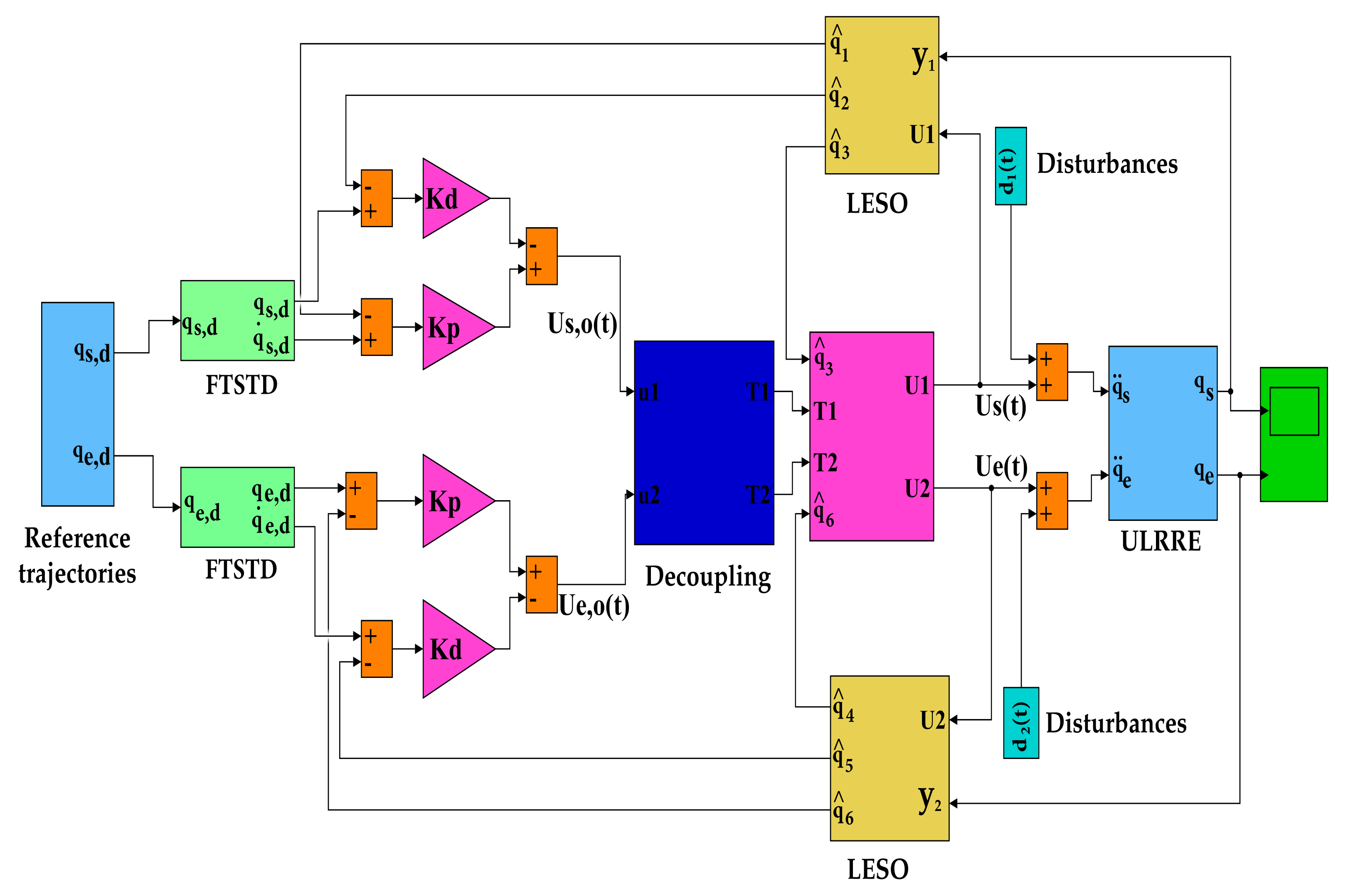
3. Topology of Proposed Method

The topology of the proposed ESO-based and FTSTD-based ADRC trajectory tracking control for ULRRE is shown in Figure 2. The MIMO system is decoupled to the single-input single-output (SISO) system, and then the proposed controller is applied. The topology consists of ESO, which removes disturbances and uncertainties as total disturbance and FTSTD to improve the system’s response.
In Figure 2, q s , d ( t ) and q e , d ( t ) represent the reference input sent to the shoulder and elbow joints, respectively. q ^ 1 ( t ) , q ^ 2 ( t ) , q ^ 4 ( t ) , and q ^ 5 ( t ) are the estimated states of LESO. q ^ 3 ( t ) and q ^ 6 ( t ) are extended states of the LESO. U s ( t ) and U e ( t ) are the control signals to ULRRE. d 1 ( t ) and d 2 ( t ) are the extrinsic disturbances. q s ( t ) and q e ( t ) represents output of shoulder and the elbow joints.

3.1. Decoupling between Shoulder and Elbow Joint

The paper aims to achieve accurate trajectory tracking for ULRRE in the presence of external disturbances and modeling uncertainties such as parameter variations. The mathematical model in Equation (1) is further expressed as:
j 11 q 1 . . + j 12 q 2 . . + c 11 q 1 . + c 12 q 2 . + g 1 + d 1 = τ 1 j 21 q 1 . . + j 22 q 2 . . + c 21 q 1 . + c 22 q 2 . + g 2 + d 2 = τ 2
where D = d 1 , d 2 T , d 1 and d 2 represent lumped disturbances. Equation (5) in state space is expressed as follows.
q 1 . . = 1 ( j 11 j 22 j 21 j 12 ) ( j 22 τ 1 j 12 τ 2 F 1 ) q 2 . . = 1 ( j 12 j 21 j 11 j 22 ) ( j 21 τ 1 j 11 τ 2 F 2 )
where
F 1 = ( j 22 c 11 j 12 c 21 ) q . 1 + ( j 22 c 12 j 12 c 22 ) q . 2 + j 22 g 1 j 12 g 2 + j 22 d 1 j 12 d 2 f 10 = ( j 22 c 11 j 12 c 21 ) q . 1 + ( j 22 c 12 j 12 c 22 ) q . 2 + j 22 g 1 j 12 g 2 f 1 d = j 22 d 1 j 12 d 2 F 1 = f 10 + f 1 d F 2 = ( j 21 c 11 j 11 c 21 ) q . 1 ( j 21 c 12 j 11 c 22 ) q . 2 j 21 g 1 + j 11 g 2 j 22 d 1 + j 12 d 2 f 20 = ( j 21 c 11 j 11 c 21 ) q . 1 ( j 21 c 12 j 11 c 22 ) q . 2 j 21 g 1 + j 11 g 2 f 2 d = j 22 d 1 + j 12 d 2 F 2 = f 20 + f 2 d
Equation (6) after simplification becomes Equation (8) and is given as:
q 1 . . = P f 1 . ( j 22 τ 1 j 12 τ 2 ) + f 1 q 2 . . = P f 1 . ( j 21 τ 1 j 11 τ 2 ) + f 2
where P f 1 = 1 ( j 11 j 22 j 21 j 12 ) , f 1 = ( f 10 + f 1 d ) P f 1 , f 2 = ( f 20 + f 2 d ) P f 1 .
After decoupling the system in Equation (8) by decoupling matrix N [52], it is written as
q . . = f + U
Here, q = [ q 1 , q 2 ] T , f = [ f 1 , f 2 ] T , U = [ U 1 , U 2 ] T = N [ τ 1 , τ 2 ] T if U is known, the control of input T = τ 1 , τ 2 T is obtained as T = N 1 U = N inv U . After separating the system, two ESO are generated for each joint using two distinct equations.
q 1 . . = f 1 + 1 ( P f 1 . j 22 ) U 1 q 2 . . = f 2 + 1 ( P f 1 . j 11 ) U 2

3.2. Finite-Time Stable Tracking Differentiator

A tracking differentiator is introduced to improve the system’s response by minimizing overshoot and enhancing noise robustness [53].It acts on input signals and avoids sudden changes by differentiating them. The performance of the ULRRE to track the trajectory has been improved by applying the FTSTD design specified in Equation (11).
z . 1 ( t ) = z 2 ( t ) z . 2 = R 2 a 1 [ z 1 v ( t ) ] 1 2 a 2 [ z 2 ( t ) R ] 2 3
a 1 and a 2 > 0. In this case, z 2 is a derivative of z 1 . The required trajectory is z 1 . R controls the rate of the transient profile and is selected as a compromise between noise tolerance and tracking precision.

3.3. Linear Extended State Observer Design

In this section, LESO is developed for a second-order system to reduce lumped disturbances. From Equation (10), the decoupled system is given by
q . . ( t ) = f 0 ( q . s ( t ) , q . e ( t ) , q s ( t ) , q e ( t ) + f d ( d ( t ) ) ) + b u ( t )
where d ( t ) is lumped disturbance, u(t) is input, q ( t ) is output, and b is the system parameter. f d ( d ( t ) ) is uncertainty resulting from both external and internal modeling and is referred to as a whole disturbance. Assume that f d ( d ( t ) ) , which represents the ULRRE’s nonlinear time-varying dynamics, is differentiable. Equations (13) and (14) are used to rewrite and express the system.
q . 1 = q 2 , q . 2 = ( f 10 + f 1 d ) P f 1 + 1 ( P f 1 . j 22 ) U 1 , q . 3 = d 1 ( q , d 1 , d . 1 ) , y 1 = q 1
q . 4 = q 5 , q . 5 = ( f 20 + f 2 d ) P f 1 + 1 ( P f 1 . j 11 ) U 2 , q . 6 = d 2 ( q , d 2 , d . 2 ) , y 2 = q 4
The LESO is designed for both of the joints individually. Two LESO are
q ^ . 1 = q ^ 2 + K 1 ( q 1 q ^ 1 ) , q ^ . 2 = q ^ 3 + K 2 ( q 1 q ^ 1 ) + 1 ( P f 1 . j 22 ) U 1 ( f 10 ) P f 1 , q ^ . 3 = K 3 ( q 1 q ^ 1 ) q ^ . 4 = q ^ 5 + K 4 ( q 4 q ^ 4 ) , q ^ . 5 = q ^ 6 + K 5 ( q 4 q ^ 4 ) + 1 ( P f 1 . j 11 ) U 2 + ( f 20 ) P f 1 , q ^ . 6 = K 6 ( q 4 q ^ 4 )
The observer gain matrices are L 1 = [ K 1 , K 2 , K 3 ] T and L 2 = [ K 4 , K 5 , K 6 ] T . All observer poles are set to w o for tuning. To calculate observer gain, the characteristic equation given below is used.
s 3 + K 1 s 2 + K 2 s + K 3 = ( s + w o ) 3 s 3 + K 4 s 2 + K 5 s + K 6 = ( s + w o ) 3
where w o is the LESO’s bandwidth. L 1 a n d L 2 , gain vectors, are expressed as K 1 = K 4 = 3 w o , K 2 = K 5 = 3 w o 2 , and K 3 = K 6 = w o 3 . A balance between tracking performance and noise tolerance is achieved by selecting an observer bandwidth w o .
ESO-based control law in general is given by u = u 0 f h , where h is the system parameter. u 0 = K p ( q 1 q 1 ) + K d ( q 2 q 2 ) + q d . . . Since K p = w c 2 and K d = 2 w c [54], with well-designed ESO, the last term in left-hand side q d . . is relatively small in a well-designed ESO. The rest of equation is a PD controller.
The feedback control law of ADRC is given by U 0 = [ U 1 , U 2 ] T = K p e + K d e . . e and e . are the state estimate errors for the position and velocity for both the joints, where q d = [ q s , d q e , d ] as reference trajectory e = [ e 1 e 2 ] T = [ ( q s , d q ^ 1 ) ( q e , d q ^ 4 ) ] T , e . = [ e 1 . e 2 . ] T = [ q ^ 2 q ^ 5 ] T . The ESO-based and FTSTD-based ADRC law for standard second-order integrator y = U 0 can be expressed as U = [ τ 1 , τ 2 ] T = N i n v ( K p e K d e . f ) , where f = [ f ^ 1 , f ^ 2 ] T are the estimate of disturbance i.e., f = >[ f 1 , f 2 >] T = [ q 3 , q 6 ] T . Controller bandwidth is determined as w c = 1 3 w o .
K p = ω c 2 0 0 ω c 2 , K d = 2 ω c 0 0 2 ω c .
As illustrated by Equation (9), the system Equation (10) eventually becomes Equation (17) with a well-designed control law.
U = N i n v ( K p e K d e . + q d . . f )

4. Stability Analysis

Provided that f ( q 1 , q 2 , , q n , u , d ( t ) , t ) is globally Lipschitz with reference to q, there appears a constant w o > 0 , w c > 0 , whereby the closed-loop system Equation (18) is asymptotically stable.
Proof. 
U = [ τ 1 , τ 2 ] T = N i n v ( K p e K d e . + q d . . f )
q s , r and q e , r are the reference trajectories for the shoulder and elbow joints. The goal is to properly track these inputs q s , d , whose derivative, q ˙ s , r , 1 , q ¨ s , r , 2 , q s , r ( n ) are bounded. Let, for the shoulder joint q s , r , 1 , q s , r , 2 , q s , r , 3 T = q ˙ s , r , q ˙ s , r , 1 , q ˙ s , r , 2 T . Define e i = q s , r , i q i , i = 1 , 2 . and q ˜ 1 = q 1 q ^ 1 , q ˜ 2 = q 2 q ^ 2 , q ˜ 3 = q 3 q ^ 3 , e 1 = q s , r , 1 q 1 , e 2 = q s , r , 2 q 2 . The proposed control law is as follows:
U 1 = [ k p ( q s , r , 1 q ^ 1 ) + k d ( q s , r , 2 q ^ 2 ) + q s , r , 3 q ^ 3 ] ( P f 1 . j 22 ) = { [ k p [ ( q s , r , 1 ( q 1 q ˜ 1 ) ] + [ k d [ ( q s , r , 2 ( q 2 q ˜ 2 ) ] + q s , r , 3 q ^ 3 } ( P f 1 . j 22 ) = [ k p ( e 1 + q ˜ 1 ) + k d [ ( e 2 + q ˜ 2 ) + q s , r , 3 q ^ 3 ] / ( P f 1 . j 22 )
It follows that for the shoulder joint
e ˙ 1 = q ˙ s , r , 1 q ˙ 1 = q s , r , 2 q 2 = e 2 , e ˙ 2 = q ˙ s , r , 2 q ˙ 2 = q s , r , 3 ( q 3 + 1 ( P f 1 . j 22 ) U 1 = q s , r , 3 q 3 [ k p ( e 1 + q ˜ 1 ) ] k d [ ( e 2 + q ˜ 2 ) q ^ 3 + q s , r , 3 ] = k p ( e 1 + q ˜ 1 ) k d [ ( e 2 + q ˜ 2 ) q ˜ 3
Let e = [ e 1 , e 2 ] T R n , q ˜ = [ q ˜ 1 , q ˜ 2 , q ˜ 3 ] T R n + 1 ; then,
e ˙ ( t ) = B e e ( t ) + B q ˜ q ˜ ( t ) B e = 0 1 k p , s k d , s and B q ˜ = 0 0 0 0 0 0 k p , s k d , s 1
Similarly, for the elbow joint,
e ˙ ( t ) = B e e ( t ) + B q ˜ q ˜ ( t ) B e = 0 1 k p , e k d , e and B q ˜ = 0 0 0 0 0 0 k p , e k d , e 1
k p , s , k d , s , k p , e and k d , e for the shoulder and elbow joints are selected to achieve s 2 + k d s + k p Hurwitz; B e is Hurwitz. To make tuning easier, let s 2 + k d s + k p = ( s + ω c ) 2 where w c > 0 . As a result, the only tuning controller parameter is w c .
lim t | | B q ˜ q ˜ ( t ) | | = 0 if h ( q , u , d , d . ) is globally Lipschitz with respect to q and lim t e ( t ) = 0 , i = 1 , 2 Q.E.D. q ˜ 1 , q ˜ 2 . . . q ˜ 5 and q ˜ 6 are the observer estimation errors. e 1 , e 2 . . . e 5 and e 6 are the controller errors. The above analysis demonstrates that the closed-loop system is asymptotically stable. ☐

5. Simulation Result Analysis
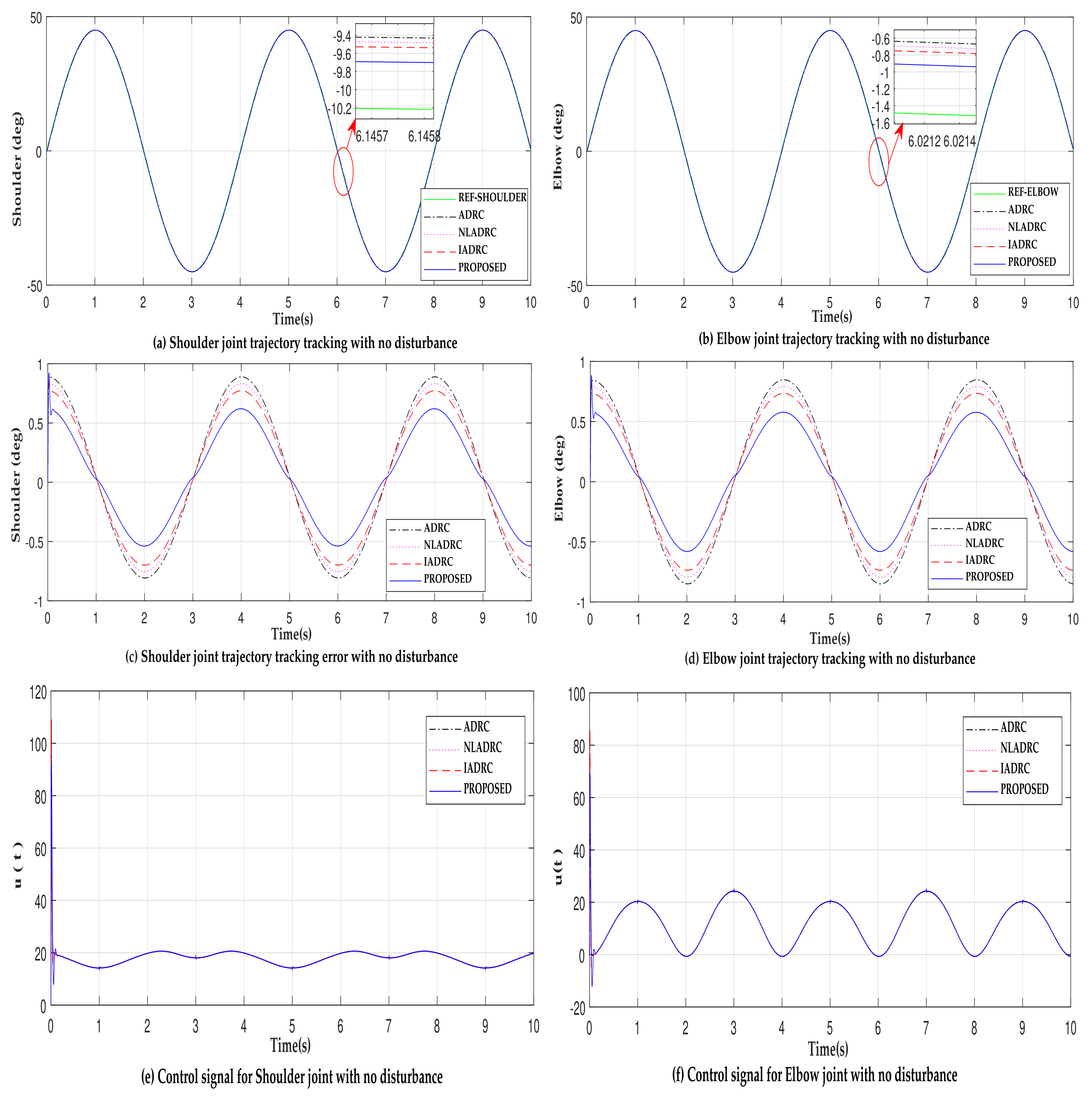
The ULRRE model is simulated with no disturbance, constant disturbance, and parameter variation to determine the effect of external disturbances and uncertainties on the controllers. The ESO and FTSTD parameters have been tuned and selected heuristically to obtain the optimal response of controllers for trajectory tracking. The method for selection of observer bandwidth for ESO was given by Dr. Gao [54] and is followed in this paper, which suggests choosing the values of observer bandwidth as a trade-off between noise sensitivity and LESO performance. Control effort tends to increase with a high value of bandwidth, which is one limitation. In this paper, the authors have chosen 400 rad/s. The proportionality and derivative constant are selected as k p = w c 2 and K d = 2 w c based on [54].
In MATLAB (2017b) [55], the controllers are evaluated in simulation under two disturbance conditions. The ode4 (Runge–Kutta) solver is employed with a sample time of 0.001 s. The shoulder and elbow joints have input trajectories of amplitude 0.7855 rad/s. The model is subjected to an external control disturbance of amplitude 5 N.m at 1.2 s. The response is recorded by applying ± 20 % parametric uncertainty and the same disturbance of 5 N.m. The performance indices such as IAE, ITE, ITAE, and ISTE played a role in the comparison of different controllers and are called generic tools for evaluation of control algorithms [56]. The lower value of performance indices indicates better performance of controller [57] and all the parameters have been selected to minimize indices values.

5.1. No Disturbance

In this case, the model of the system has been simulated without incorporating external disturbance. The accompanying Figure 3 shows a comparison of previously existing techniques with the proposed method in trajectory tracking, the error plots, and control signal.
In Figure 3, when no disturbance is given to the system, the minimized plots (a) and (b) display performance of IADRC, NLADRC, ADRC, and the proposed method while reference trajectory tracking for shoulder and elbow joints. The minimized plots (c) and (d) depict the error trajectory generated during reference tracking. The control signal required by the controllers is illustrated in the minimized plots (e) and (f).
Minimum values of ITSE, ISE, ITAE, and IAE indicate the proposed method performs better in terms of trajectory tracking for ULRRE and can be observed from Table 3.
ITSE, ISE, ITAE, and IAE of the proposed method has values 7.515, 1.516, 16.83 and 3.374 for the shoulder joint and 7.499, 1.509, 16.88, and 3.383 for the elbow joint respectively which are minimum as compared IADRC, NLADRC, and ADRC.

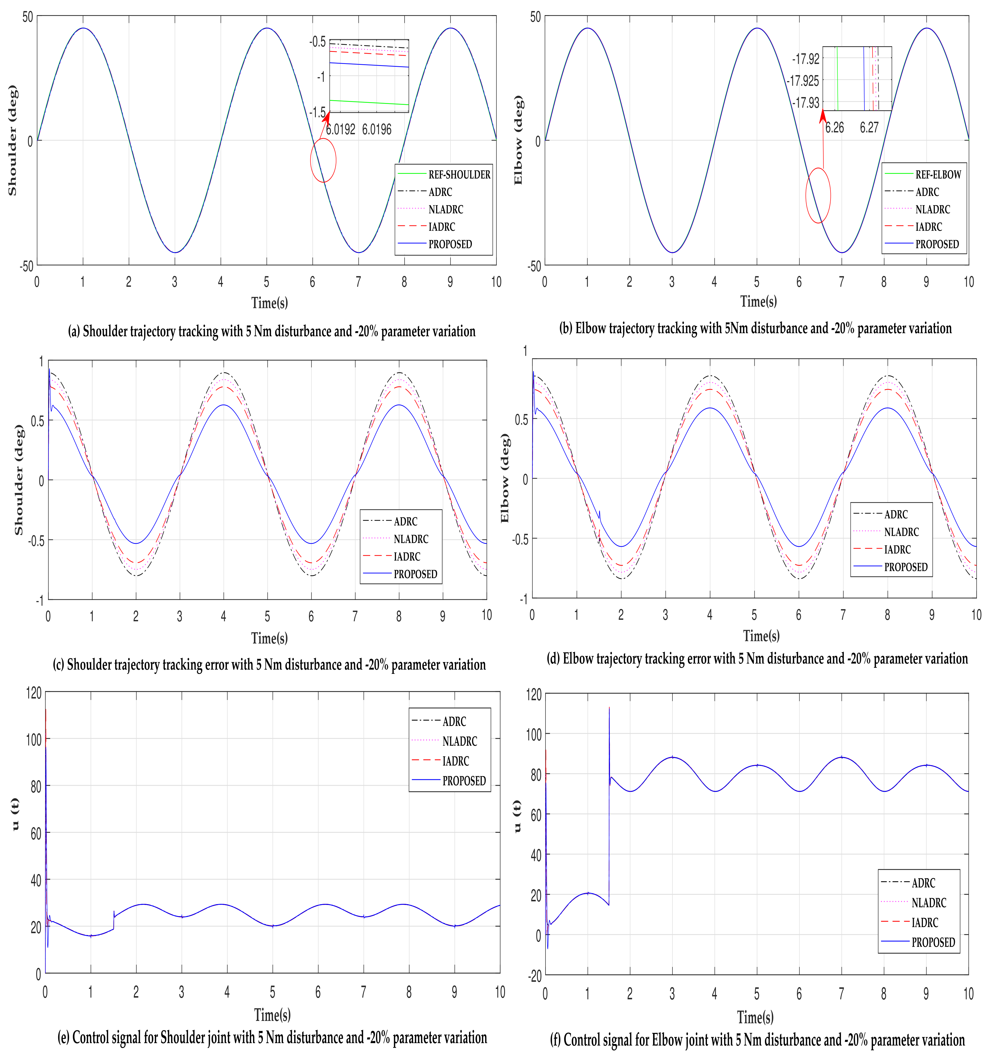
5.2. Effect of Disturbance and Parameter Variations

To assess the efficacy of controllers, a parametric uncertainty of ± 20 % is added. The parameters of changed values with g value maintained constant as 9.81 m/s 2 are listed in Table 4. Table 5 and Table 6 show the after-effects of these uncertainty. To evaluate the ability of disturbance rejection, the proposed method, along with the other ESO-based methods, has been tested with a constant disturbance of 5 N.m. at t = 1.2 s.
In Figure 4, when constant disturbance with 20 % parameter variation is given to the system, the minimized plots (a) and (b) display the performance of IADRC, NLADRC, ADRC, and the proposed method while reference trajectory tracking for shoulder and elbow joints. The minimized plots (c) and (d) depict the error trajectory generated during reference tracking. The control signal required by the controllers is illustrated in the minimized plots (e) and (f).
In Figure 5, when constant disturbance with +20% parameter variation is given to the system, the minimized plots (a) and (b) display the performance of IADRC, NLADRC, ADRC, and the proposed method while reference trajectory tracking for shoulder and elbow joints. The minimized plots (c) and (d) depict the error trajectory generated during reference tracking. The control signal required by the controllers is illustrated in the minimized plots (e) and (f).
The ITSE, ISE, ITAE, and IAE of the proposed method have values 7.529, 13.61, 15.73, and 18 with − 20 % parameter variation and 7.534, 13.61, 13.74, and 18 for the shoulder joint with + 20 % parameter variation, respectively, which are minimum as compared IADRC, NLADRC, and ADRC. Minimum values of ITSE, ISE, ITAE, and IAE indicate the proposed method performs better in terms of trajectory tracking for ULRRE and can be observed from Table 5.
The ITSE, ISE, ITAE, and IAE of the proposed method have values 7.501, 13.59, 15.71, and 17.97 with 20 % parameter variation and 7.522, 13.60, 15.72, and 17.99 for the elbow joint with + 20 % parameter variation, respectively, which are minimum as compared IADRC, NLADRC, and ADRC. Minimum values of ITSE, ISE, ITAE, and IAE indicate the proposed method performs better in terms of trajectory tracking for ULRRE and can be observed form the Table 6.
It has been observed that all the techniques mentioned above can reject disturbances. The proposed method outperforms all others in terms of trajectory tracking with disturbance rejection, as evidenced by consistent performance indices under the introduction of parametric uncertainties and disturbances. In comparison to previous ESO-based approaches, the proposed controller shows promise.

6. Discussion

Robotic-assisted rehabilitation is a boon to those with upper and lower limb disabilities, as well as the medical community. Better control methods used in these devices to carry out rehabilitative activities may physically improve the patient’s condition. Trajectory tracking is one such activity that assists patients in their early recovery by allowing them to train their targeted joints continually. Trajectory monitoring improves muscular mobility through training. The researchers are driven to advance an exoskeleton in medicine because it can treat patients more conveniently and efficiently than standard rehabilitation approaches.
Control engineering plays a crucial role in increasing the capacity of these devices using various efficient control algorithms and allowing the system to track or behave as per the required performance, which is a significant challenge. This article attempts to enhance one such performance, i.e., the ULRRE trajectory tracking. This research presents a simulation study that addresses the trajectory tracking control problem for a two-degrees of freedom ULRRE that models the human upper limb, including the shoulder and elbow joints. The simulation tests the effectiveness of ESO-based methods used for rehabilitation tracking applications [40,51,52]. The investigated disturbance and parameter variation case studies on ULRRE determine the controllers’ robustness as mentioned above while performing trajectory tracking. When a disturbance is given to the system, the error plots for the ADRC, NLADRC, IADRC, and proposed method reveal that ESO-based controllers exhibit disturbance rejection capabilities. The results show precise trajectory tracking in no disturbance and with disturbance case, where all ESO-based methods requires nearly identical control signal levels.
The proposed control method utilizes the combination of LESO and FTSTD, whereas IADRC [52] uses ESO nonlinear state error feedback (NLSEF) and tracking differentiator (TD), which is complex in design as the number of parameters for tuning increases. NLADRC [51] uses nonlinear ESO and NLSEF, which has fewer parameters to tune than IADRC and the proposed method. ADRC [40] uses the ESO and has the minor tuning parameters among all controllers. From the results, the performance indices indicate that the proposed methods enhance the system’s performance by tracking accurate trajectory and reducing the trajectory tracking error than IADRC, NLADRC, and ADRC. The proposed controller is less complex than IADRC, as it only uses ESO and FTSTD to achieve better accuracy than IADRC. In ESO-based methods, choosing observer bandwidth is critical. It affects the tracking error, which tends to decrease with the increase in observer bandwidth, but it inversely affects the control effort, increasing bandwidth. The observer bandwidth is chosen as a trade-off between the tracking performance and control signal requirement and is one of the limitations of this model and ESO-based methods.
The proposed method will compare the presented ESO-based approaches to the proposed method in the future. The test technique will be designed and put to the test in a controlled laboratory environment. Healthy and challenged individuals will be asked to complete ten cycles of trajectory exercise using the gadget for each controller. Meanwhile, after each repetition, a 5-min rest is provided for relaxation. A sinusoidal motion will be given as input to the device, and the output trajectory will be recorded by angular measurement devices such as encoders and preserved for analysis. The exoskeleton connects to the upper hand by connecting cuffs attached to two joints. The control enclosure will hold an embedded computer, rotary actuators, encoders, and a power supply. The computer will instruct the actuators to use generated control signals to drive the ULRRE. The motions of the joints are then recorded and analyzed by using encoders. The algorithm’s scope is not restricted to the present application; it may apply to other control applications.

7. Conclusions

In this article, we present a novel method for tracking ULRRE trajectories accurately. The study provides a method for combining ESO and FTSTD that enhances tracking, rejects external disturbances, and shows robustness against parametric uncertainties of ± 20 % . The developed method is compared to pre-existing ESO-based methods such as ADRC, NLADRC, and I-ADRC. The performance indices quantify the new method’s efficiency compared to existing ESO-based strategies established for rehabilitation exoskeletons. A sagittal plane trajectory tracking on a 2 DoF ULRRE with shoulder and elbow joint has been simulated, compared, and discussed. In the future, experiments will be conducted to validate the proposed method.

Author Contributions

Conceptualization, S.A.; methodology, S.A. and I.E.; software, S.A.; validation, S.A.; formal analysis, S.A.; investigation, writing—original draft preparation, S.A.; writing—review and editing, S.A., I.E. and T.B.; supervision, L.W., B.P., F.M. and S.S.; project administration, I.E.; funding acquisition, I.E. All authors have read and agreed to the published version of the manuscript.

Funding

Funds for this research was provided by Universiti Teknologi PETRONAS (UTP) Malaysia, under research Grants 0153AB-M66 and 015LC0-243.

Institutional Review Board Statement

Not applicable.

Informed Consent Statement

Not applicable.

Data Availability Statement

Not applicable.

Acknowledgments

The authors would like to thank Universiti Teknologi PETRONAS (UTP) Malaysia, Shri Guru Gobind Singhji Institute of Engineering and Technology, Nanded, India, University of Burgundy, Dijon, France, and University of Technology, Sydney (UTS) for their support.

Conflicts of Interest

The authors declare no conflict of interest.

References

  1. Qian, C.; Li, W.; Jia, T.; Li, C.; Lin, P.J.; Yang, Y.; Ji, L. Quantitative Assessment of Motor Function by an End-Effector Upper Limb Rehabilitation Robot Based on Admittance Control. Appl. Sci. 2021, 11, 6854. [Google Scholar] [CrossRef]
  2. Miao, Q.; Zhang, M.; Cao, J.; Xie, S.Q. Reviewing high-level control techniques on robot-assisted upper-limb rehabilitation. Adv. Robot. 2018, 32, 1253–1268. [Google Scholar] [CrossRef]
  3. Nguiadem, C.; Raison, M.; Achiche, S. Motion Planning of Upper-Limb Exoskeleton Robots: A Review. Appl. Sci. 2020, 10, 7626. [Google Scholar] [CrossRef]
  4. Jakob, I.; Kollreider, A.; Germanotta, M.; Benetti, F.; Cruciani, A.; Padua, L.; Aprile, I. Robotic and sensor technology for upper limb rehabilitation. PM&R 2018, 10, S189–S197. [Google Scholar]
  5. Lo, H.S.; Xie, S.Q. Exoskeleton robots for upper-limb rehabilitation: State of the art and future prospects. Med. Eng. Phys. 2012, 34, 261–268. [Google Scholar] [CrossRef] [PubMed]
  6. Guo, Z.; Yu, H.; Yin, Y.H. Developing a mobile lower limb robotic exoskeleton for gait rehabilitation. J. Med. Devices 2014, 8, 044503. [Google Scholar] [CrossRef]
  7. Zhang, L.; Guo, S.; Sun, Q. An assist-as-needed controller for passive, assistant, active, and resistive robot-aided rehabilitation training of the upper extremity. Appl. Sci. 2021, 11, 340. [Google Scholar] [CrossRef]
  8. Su, Y.; Sun, D.; Ren, L.; Mills, J.K. Integration of saturated PI synchronous control and PD feedback for control of parallel manipulators. IEEE Trans. Robot. 2006, 22, 202–207. [Google Scholar]
  9. Taha, Z.; Majeed, A.P.A.; Abidin, A.F.Z.; Ali, M.A.H.; Khairuddin, I.M.; Deboucha, A.; Tze, M.Y.W.P. A hybrid active force control of a lower limb exoskeleton for gait rehabilitation. Biomed. Tech. Eng. 2018, 63, 491–500. [Google Scholar] [CrossRef]
  10. Spong, M.W.; Hutchinson, S.; Vidyasagar, M. Robot modeling and control. IEEE Control Syst. 2006, 26, 113–115. [Google Scholar]
  11. Lu, R.; Li, Z.; Su, C.Y.; Xue, A. Development and learning control of a human limb with a rehabilitation exoskeleton. IEEE Trans. Ind. Electron. 2013, 61, 3776–3785. [Google Scholar] [CrossRef]
  12. Jamwal, P.K.; Xie, S.Q.; Hussain, S.; Parsons, J.G. An adaptive wearable parallel robot for the treatment of ankle injuries. IEEE/ASME Trans. Mechatron. 2012, 19, 64–75. [Google Scholar] [CrossRef]
  13. Kazerooni, H.; Racine, J.L.; Huang, L.; Steger, R. On the control of the berkeley lower extremity exoskeleton (BLEEX). In Proceedings of the 2005 IEEE International Conference on Robotics and Automation, Barcelona, Spain, 18–22 April 2005; pp. 4353–4360. [Google Scholar]
  14. Kazerooni, H.; Chu, A.; Steger, R. That which does not stabilize, will only make us stronger. Int. J. Robot. Res. 2007, 26, 75–89. [Google Scholar] [CrossRef] [Green Version]
  15. Yang, Z.; Zhu, Y.; Yang, X.; Zhang, Y. Impedance control of exoskeleton suit based on adaptive RBF neural network. In Proceedings of the 2009 International Conference on Intelligent Human-Machine Systems and Cybernetics, Hangzhou, China, 26–27 August 2009; Volume 1, pp. 182–187. [Google Scholar]
  16. Li, S.; Yang, J.; Chen, W.H.; Chen, X. Disturbance observer-based control: Methods and applications. In Proceedings of the 2016 International Conference on Unmanned Aircraft Systems (ICUAS), Arlington, VA, USA, 7–10 June 2016. [Google Scholar]
  17. Gao, Z.; Huang, Y.; Han, J. An alternative paradigm for control system design. In Proceedings of the 40th IEEE Conference on Decision and Control, Orlando, FL, USA, 4–7 December 2001; Volume 5, pp. 4578–4585. [Google Scholar]
  18. Gao, Z.; Hu, S.; Jiang, F. A novel motion control design approach based on active disturbance rejection. In Proceedings of the 40th IEEE Conference on Decision and Control, Orlando, FL, USA, 4–7 December 2001; Volume 5, pp. 4877–4882. [Google Scholar]
  19. Tian, G.; Gao, Z. Benchmark tests of active disturbance rejection control on an industrial motion control platform. In Proceedings of the 2009 American Control Conference, St. Louis, MO, USA, 10–12 June 2009; pp. 5552–5557. [Google Scholar]
  20. Su, Y.X.; Duan, B.Y.; Zheng, C.H.; Zhang, Y.F.; Chen, G.D.; Mi, J.W. Disturbance-rejection high-precision motion control of a Stewart platform. IEEE Trans. Control Syst. Technol. 2004, 12, 364–374. [Google Scholar] [CrossRef]
  21. Ginhoux, R.; Gangloff, J.; de Mathelin, M.; Soler, L.; Sanchez, M.M.A.; Marescaux, J. Active filtering of physiological motion in robotized surgery using predictive control. IEEE Trans. Robot. 2005, 21, 67–79. [Google Scholar] [CrossRef] [Green Version]
  22. Zhu, E.; Pang, J.; Sun, N.; Gao, H.; Sun, Q.; Chen, Z. Airship horizontal trajectory tracking control based on Active Disturbance Rejection Control (ADRC). Non-Linear Dyn. 2013, 75, 725–734. [Google Scholar] [CrossRef]
  23. Qin, C.; Qi, N.; Lü, R.; Zhu, K. ADRC fractional order PID controller design of hypersonic flight vehicle. Trans. Nanjing Univ. Aeronaut. Astronaut. 2011, 28, 240–244. [Google Scholar]
  24. Desai, R.; Patre, B.M.; Pawar, S.N. Active disturbance rejection control with adaptive rate limitation for process control application. In Proceedings of the 2018 Indian Control Conference (ICC), Kanpur, India, 4–6 January 2018; pp. 131–136. [Google Scholar]
  25. Huang, Y.; Xue, W. Active disturbance rejection control: Methodology and theoretical analysis. ISA Trans. 2014, 53, 963–976. [Google Scholar] [CrossRef]
  26. Yu, T.; Chan, K.W.; Tong, J.P.; Zhou, B.; Li, D.H. Coordinated robust non-linear boiler-turbine-generator control systems via approximate dynamic feedback linearization. J. Process. Control 2010, 20, 365–374. [Google Scholar] [CrossRef]
  27. Huang, C.E.; Li, D.; Xue, Y. Active disturbance rejection control for the ALSTOM gasifier benchmark problem. Control Eng. Pract. 2013, 21, 556–564. [Google Scholar] [CrossRef]
  28. Dulf, E.H.; Both, R.; Muresan, C.I. Active disturbance rejection controller for a separation column. In Proceedings of the 2014 IEEE International Conference on Automation, Quality and Testing, Robotics, Cluj-Napoca, Romania, 22–24 May 2014; pp. 1–6. [Google Scholar]
  29. Tan, W.; Fu, C. Linear active disturbance-rejection control: Analysis and tuning via IMC. IEEE Trans. Ind. Electron. 2016, 63, 2350–2359. [Google Scholar] [CrossRef]
  30. Garran, P.T.; Garcia, G. Design of an optimal PID controller for a coupled tanks system employing ADRC. IEEE Lat. Am. Trans. 2017, 15, 189–196. [Google Scholar] [CrossRef]
  31. Pawar, S.N.; Chile, R.H.; Patre, B.M. Modified reduced order observer based linear active disturbance rejection control for TITO systems. ISA Trans. 2017, 71, 480–494. [Google Scholar] [CrossRef] [PubMed]
  32. Madonski, R.; Nowicki, M.; Przemys, l.H. Application of active disturbance rejection controller to water supply system. In Proceedings of the 33rd Chinese Control Conference, Nanjing, China, 28–30 July 2014; pp. 4401–4405. [Google Scholar]
  33. Zheng, Q.; Gao, Z. An energy saving, factory-validated disturbance decoupling control design for extrusion processes. In Proceedings of the 10th World Congress on Intelligent Control and Automation, Beijing, China, 6–8 July 2012; pp. 2891–2896. [Google Scholar]
  34. Zeng, D.; Yu, Z.; Xiong, L.; Fu, Z.; Li, Z.; Zhang, P.; Leng, B.; Shan, F. HFO-LADRC lateral motion controller for autonomous road sweeper. Sensors 2020, 20, 2274. [Google Scholar] [CrossRef] [PubMed]
  35. Li, D.; Ding, P.; Gao, Z. Fractional active disturbance rejection control. ISA Trans. 2016, 62, 109–119. [Google Scholar] [CrossRef] [PubMed]
  36. Han, J. From PID to active disturbance rejection control. IEEE Trans. Ind. Electron. 2009, 56, 900–906. [Google Scholar] [CrossRef]
  37. Han, J. Auto-disturbances-rejection controller and its applications. Control Decis. 1998, 13, 19–23. (In Chinese) [Google Scholar]
  38. Gao, Z. Active disturbance rejection control: A paradigm shift in feedback control system design. In Proceedings of the American Control Conference 2006, Minneapolis, MN, USA, 14–16 June 2006; p. 7. [Google Scholar]
  39. Viteckova, S.; Kutilek, P.; Jirina, M. Wearable lower limb robotics: A review. Biocybern. Biomed. Eng. 2013, 33, 96–105. [Google Scholar] [CrossRef]
  40. Long, Y.; Du, Z.; Cong, L.; Wang, W.; Zhang, Z.; Dong, W. Active disturbance rejection control based human gait tracking for lower extremity rehabilitation exoskeleton. ISA Trans. 2017, 67, 389–397. [Google Scholar] [CrossRef]
  41. Guerrero-Castellanos, J.F.; Rifa, H.; Arnez-Paniagua, V.; Linares-Flores, J.; Saynes-Torres, L.; Mohammed, S. Robust Active Disturbance Rejection Control via Control Lyapunov Functions: Application to Actuated-Ankle-Foot-Orthosis. Control Eng. Pract. 2018, 80, 49–60. [Google Scholar] [CrossRef]
  42. Meng, W.; Liu, Q.; Zhou, Z.; Ai, Q.; Sheng, B.; Xie, S.S. Recent development of mechanisms and control strategies for robot-assisted lower limb rehabilitation. Mechatronics 2015, 31, 132–145. [Google Scholar] [CrossRef]
  43. Roman, R.C.; Precup, R.E.; Bojan-Dragos, C.A.; Szedlak-Stinean, A.I. Combined Model-Free Adaptive Control with Fuzzy Component by Virtual Reference Feedback Tuning for Tower Crane Systems. Procedia Comput. Sci. 2019, 162, 267–274. [Google Scholar] [CrossRef]
  44. Zhang, H.; Liu, X.; Ji, H.; Hou, Z.; Fan, L. Multi-Agent-Based Data-Driven Distributed Adaptive Cooperative Control in Urban Traffic Signal Timing. Energies 2019, 12, 1402. [Google Scholar] [CrossRef] [Green Version]
  45. Joe, H.M.; Oh, J.H. A Robust Balance-Control Framework for the Terrain-Blind Bipedal Walking of a Humanoid Robot on Unknown and Uneven Terrain. Sensors 2019, 19, 4194. [Google Scholar] [CrossRef] [Green Version]
  46. Hassan, M.; Kadone, H.; Suzuki, K.; Sankai, Y. Wearable gait measurement system with an instrumented cane for exoskeleton control. Sensors 2014, 14, 1705–1722. [Google Scholar] [CrossRef] [PubMed] [Green Version]
  47. Del-Ama, A.J.; Moreno, J.C.; Gil-Agudo, A.; De-los Reyes, A.; Pons, J.L. Online assessment of human-robot interaction for hybrid control of walking. Sensors 2012, 12, 215–225. [Google Scholar] [CrossRef] [PubMed] [Green Version]
  48. Long, Y.; Du, Z.J.; Wang, W.D.; Dong, W. Robust sliding mode control based on GA optimization and CMAC compensation for lower limb exoskeleton. Appl. Bionics Biomech. 2016, 2016, 5017381. [Google Scholar] [CrossRef] [PubMed] [Green Version]
  49. Chen, G.; Chan, C.K.; Guo, Z.; Yu, H. A review of lower extremity assistive robotic exoskeletons in rehabilitation therapy. Crit. Rev. Biomed. Eng. 2013, 41, 4–5. [Google Scholar] [CrossRef] [PubMed]
  50. Bortole, M.; Venkatakrishnan, A.; Zhu, F.; Moreno, J.C.; Francisco, G.E.; Pons, J.L.; Contreras-Vidal, J.L. The H2 robotic exoskeleton for gait rehabilitation after stroke: Early findings from a clinical study. J. Neuroeng. Rehabil. 2015, 12, 54. [Google Scholar] [CrossRef] [PubMed] [Green Version]
  51. Aole, S.; Elamvazuthi, I.; Waghmare, L.; Patre, B.; Meriaudeau, F. Non-linear active disturbance rejection control for upper limb rehabilitation exoskeleton. Proc. Inst. Mech. Eng. Part I J. Syst. Control Eng. 2021, 235, 606–632. [Google Scholar] [CrossRef]
  52. Aole, S.; Elamvazuthi, I.; Waghmare, L.; Patre, B.; Meriaudeau, F. Improved active disturbance rejection control for trajectory tracking control of lower limb robotic rehabilitation exoskeleton. Sensors 2020, 20, 3681. [Google Scholar] [CrossRef] [PubMed]
  53. Guo, B.-Z.; Zhao, Z.-L. Active Disturbance Rejection Control for Non-Linear Systems: An Introduction; John Wiley & Sons: Hoboken, NJ, USA, 2016. [Google Scholar]
  54. Gao, Z. Scaling and bandwidth-parameterization based controller tuning. In Proceedings of the American Control Conference, Minneapolis, MN, USA, 14–16 June 2006; Volume 6, pp. 4989–4996. [Google Scholar]
  55. MATLAB/Simulink (2017b, The Mathworks, Inc., Natick, MA, USA). Available online: https://www.mathworks.com/products/matlab.html (accessed on 1 November 2021).
  56. Tavazoei, M.S. Notes on integral performance indices in fractional-order contro systems. J. Process Control 2010, 20, 285–291. [Google Scholar] [CrossRef]
  57. Dorf, R.C.; Bishop, R.H. Modern Control Systems; Pearson: London, UK, 2011. [Google Scholar]
Figure 1. Upper limb robotic rehabilitation exoskeleton.
Applsci 12 01287 g001
Figure 2. Topology of proposed ESO-based and FTSTD-based ADRC trajectory tracking control for ULRRE.
Applsci 12 01287 g002
Figure 3. Sinusoidal trajectory tracking comparison of ADRC, NLADRC, IADRC, and the proposed method for the shoulder and elbow joints with a reference without disturbance.
Applsci 12 01287 g003
Figure 4. Sinusoidal trajectory tracking comparison of ADRC, NLADRC, IADRC, and the proposed method for the shoulder and elbow joints with 20 % parameter variation and constant disturbance.
Applsci 12 01287 g004
Figure 5. Sinusoidal trajectory tracking comparison of ADRC, NLADRC, IADRC, and the proposed method for the shoulder and elbow joints with +20% parameter variation and constant disturbance.
Applsci 12 01287 g005
Table 1. Model parameter.
Upper Limb ParametersParameterValueUnits
Limb and exoskeleton masses m 1 2.25kg
m 2 1.47kg
Limb lengths L 1 0.34m
L 2 0.25m
Center of mass L c 1 0.25m
L c 2 0.125m
Mass moment of inertia for exoskeleton and limbs I 1 0.2505kg·m 2
I 2 0.0925kg·m 2
Table 2. Nomenclature.
NotationDescription
J ( q ) R 2 × 2 Inertia matrix.
C ( q , q . ) R 2 × 2 Coriolis and centrifugal force matrix.
G R 2 × 1 Gravitational force matrix.
T R 2 × 1 Control input vector.
D R 2 × 1 Denotes unmodeled dynamics and external disturbances matrix.
q = [ q 1 q 2 ] T q 1 and q 2 angle traced by shoulder and elbow joints.
T = [ τ 1 τ 2 ] T τ 1 and τ 2 are torques of both the joints.
Table 3. Performance indices for the proposed method, IADRC, NLADRC, and ADRC for the shoulder and the elbow joint in no disturbance case.
Control Method ProposedIADRC [52]NLADRC [51]ADRC [40]
Joints ShoulderElbowShoulderElbowShoulderElbowShoulderElbow
Performance
indices
ITSE (Deg.)7.5157.49913.613.5915.7215.7117.9817.97
ISE (Deg.)1.5161.5092.7272.7213.153.1433.6033.595
ITAE (Deg.)16.8316.8823.4823.5125.2125.2326.9626.99
IAE (Deg.)3.3743.3834.7024.7045.0465.0485.3975.399
Table 4. Parameters of the ULRRE.
Upper Limb ParametersParameterActual Value 20 % + 20 % Units
Limb and exoskeleton masses m 1 2.251.82.7kg
m 2 1.471.1761.764kg
Limb lengths L 1 0.340.2720.408m
L 2 0.250.20.3m
Center of mass L c 1 0.170.1360.204m
L c 2 0.1250.10.15m
Mass moment of inertia
for exoskeleton and limbs
I 1 0.25050.20040.3006kg·m 2
I 2 0.09250.0740.111kg·m 2
Table 5. Performance indices of the shoulder joint ±20% parameter variation and constant disturbance.
Shoulder Joint
ITSE (Deg.)ISE (Deg.)ITAE (Deg.)IAE (Deg.)
Control
method
−20%+20%−20%+20%−20%+20%−20%+20%
Proposed7.5297.5341.521.5216.8316.843.3773.379
IADRC [52]13.6113.612.732.7323.4823.494.7034.703
NLADRC [51]15.7315.743.1543.15425.2125.215.0475.048
ADRC [40]18183.6073.60726.9626.975.3985.399
Table 6. Performance indices of the elbow joint ± 20 % parameter variation and constant disturbance.
Elbow Joint
ITSE (Deg.)ISE (Deg.)ITAE (Deg.)IAE (Deg.)
Control
method
−20%+20%−20%+20%−20%+20%−20%+20%
Proposed7.5017.5221.511.51616.8816.933.3833.395
IADRC [52]13.5913.602.7212.72623.5023.514.7034.707
NLADRC [51]15.7115.723.1443.14925.2325.245.0475.052
ADRC [40]17.9717.993.5963.60226.98275.3985.403
Publisher’s Note: MDPI stays neutral with regard to jurisdictional claims in published maps and institutional affiliations.

