Identification of a Suitable Machine Learning Model for Detection of Asymptomatic Ganoderma boninense Infection in Oil Palm Seedlings Using Hyperspectral Data

Abstract

In Malaysia, oil palm industry has made an enormous contribution to economic and social prosperity. However, it has been affected by basal stem rot (BSR) disease caused by Ganoderma boninense (G. boninense) fungus. The conventional practice to detect the disease is through manual inspection by a human expert every two weeks. This study aimed to identify the most suitable machine learning model to classify the inoculated (I) and uninoculated (U) oil palm seedlings with G. boninense before the symptoms’ appearance using hyperspectral imaging. A total of 1122 sample points were collected from frond 1 and frond 2 of 28 oil palm seedlings at the age of 10 months old, with 540 and 582 reflectance spectra extracted from U and I seedlings, respectively. The significant bands were identified based on the high separation between U and I seedlings, where the differences were observed significantly in the NIR spectrum. The reflectance values of each selected band were later used as input parameters of the 23 machine learning models developed using decision trees, discriminant analysis, logistic regression, naïve Bayes, support vector machine (SVM), k-nearest neighbor (kNN), and ensemble modelling with various types of kernels. The bands were optimized according to the classification accuracy achieved by the models. Based on the F-score and performance time, it was demonstrated that coarse Gaussian SVM with 9 bands performed better than the models with 35, 18, 14, and 11 bands. The coarse Gaussian SVM achieved an F-score of 95.21% with a performance time of 1.7124 s when run on a personal computer with an Intel^® Core™ i7-8750H processor and 32 GB RAM. This early detection could lead to better management in the oil palm industry.

1. Introduction

Oil palm (Elaeis guineensis) is a palm species that has been extensively planted in Southeast Asia, primarily in Indonesia and Malaysia, to fulfil the global demand for vegetable oil due to the increasing population, income, and growing biofuel market. In Malaysia, oil palm is the main commodity crop that has significantly contributed to the country’s economic development and stability. Furthermore, the increasing exports of palm-based products such as palm oil, palm kernel oil, palm kernel cake and palm-based oleochemicals maintain Malaysia as the second-largest exporter in the world.

Nevertheless, in Southeast Asia, oil palm has been affected by basal stem rot (BSR) disease caused by white-rot fungus identified as Ganoderma boninense (G. boninense). BSR is a soil-borne disease that once infected only mature trees; however, the study by Sanderson [1] reported that seedlings are also susceptible to the infection whereby the symptoms appear earlier and more severe. G. boninense cultivates through uninjured roots and produces enzymes that could degrade the woody tissues, cellulose, lignin layers, and xylem, causing a major disruption in water and nutrients distribution to the top part of the palm [2,3,4]. In brief, the earliest symptoms in oil palm seedlings can be detected by the appearance of fungal mass, followed by yellowing and necrosis of older leaves [5]. In severe cases, the infection could cause stunted growth, especially in height, girth and frond count due to the inability to perform photosynthesis. However, the appearance of fungal mass is difficult to examine by naked eyes and can often be overlooked because it may present or may not present before or after the yellowing of leaves [6,7].

Consequently, Malaysia has reported annual losses of up to RM 1.5 billion due to this disease, making BSR the most economically devastating disease in oil palm plantations. Based on the BSR incident rate, the total area affected in 2020 was estimated to be 443,440 hectares, equivalent to 65.6 million oil palms, which is worrying if preventive measures are not implemented [8]. According to Idris et al. [7], G. boninense infection could cause 80% of the affected trees to die and 25% to 40% yield losses. However, the trees with less than 20% infection can still be treated [9]. Therefore, it is crucial to detect the BSR disease at an early stage to ensure sufficient time for proper treatments, which hence prevent the disease from spreading.

Laboratory-based methods are considered reliable for early detection of G. boninense. However, these methods involve stem collections that may cause injuries to trees that lead to destruction. Meanwhile, sensor-based methods for BSR detection are widely studied, but these methods are time-consuming and impractical for large-scale plantations. Hyperspectral imaging provides a solution by its ability to cover large areas in a single imaging session. This device has been employed by Helmi and Mohanad [10], Shafri and Hamdan [11], Shafri et al. [12], Izzuddin et al. [13], and Izzuddin et al. [14] to detect BSR disease in oil palm plantations. These studies used hyperspectral reflectance data to calculate vegetation indices and optimize spectral indices to differentiate between different healthiness levels of oil palm trees. Shafri et al. [12] developed the best approach, which used a combination of red (610.5 nm) and NIR (738 nm) bands to formulate optimized spectral indices. As a result, the ratio of red and NIR bands and the normalized difference vegetation index a (NDVIa) had an overall accuracy of 86%. Based on this research, it can be concluded that hyperspectral imaging is an excellent tool for detecting BSR disease in oil palms.

Machine learning techniques have been applied widely in many fields, such as speech recognition [15,16] and remote sensing land cover detection [17,18]. In recent years, the agricultural field has also started to take advantage of machine learning capability. For example, in crop yield estimation [19], disease detection [20], weed detection [21], crop quality [22], species recognition [23], animal welfare [24], livestock production [25], water management [26] and soil management [27].

Further, machine learning application in G. boninense detection in mature oil palms was started by Lelong et al. [28] in North Sumatra, Indonesia. Leaves reflectance was collected using a Unispec spectroradiometer (PP Systems, Amesbury, MA, USA) that covers from 310–1130 nm. However, only reflectance spectra from 450–1000 nm were included and smoothed using the Savitzky–Golay method prior to the development of the partial least square discriminant analysis (PLS-DA) classification model. The PLS-DA yielded a classification accuracy of 94% in classifying healthy trees and trees with different levels of G. boninense infection. Next, Liaghat et al. [29] carried out early detection of G. boninense in 15 years old oil palm trees. Reflectance spectra were taken from frond number 17 of healthy (T0), mild (T1), medium (T2), and severely (T3) infected trees using an ASD field spectroradiometer (Analytical Spectral Devices Inc., Boulder, CO, USA). The infections were confirmed using a polymerase chain reaction (PCR) test. The reflectance spectra were then smoothed and transformed into the first and second derivatives spectra using the Savitzky–Golay method. It can be observed that NIR reflectance was significantly reduced as the disease severity increased. The data were reduced using principal component analysis (PCA). Naïve Bayes classification model predicted the diseased trees with 96% accuracy using raw reflectance spectra, while kNN yielded 97% using the first and second derivative data.

Meanwhile, Liaghat et al. [30] collected the absorbance data of T0, T1, T2 and T3 infected oil palms using a Fourier transform infrared spectroscopy (FT-IR) spectrometer (Thermo Fisher Scientific Inc., Waltham, MA, USA). The data were obtained from frond number 17 and transformed into the first and second derivatives using the Savitzky–Golay method after baseline correction and normalization. The dimensionality of the data was reduced using PCA before classification models were developed based on the best principal components to classify the different levels of G. boninense infections. The result showed that the linear discriminant analysis (LDA) model showed the highest overall classification accuracy of 92% when using the raw absorbance dataset. In addition, Ahmadi et al. [31] acquired the reflectance spectra of frond number 9 and 17 of 12 years old oil palm trees using GER 1500 handheld spectrometer (Geophysical and Environmental Research Corporation, Millbrook, NY, USA). The study focused on the early detection of BSR; thus, the reflectance spectra were obtained only from T0 and T1 infected trees. The artificial neural network (ANN) was applied to discriminate between the T0 and T1 using raw, first and second derivative spectra. The raw reflectance spectra between 550 and 556 nm produced 100% classification accuracy for T1, while the first derivative reflectance has yielded 100% accuracy for T1 and 83% accuracy for T0.

Furthermore, Khaled et al. [32] utilized dielectric spectroscopy to obtain impedance, capacitance, dielectric constant and dissipation factor to detect G. boninense in oil palm plantation. The dielectric properties of T0, T1, T2 and T3 diseased trees were reduced using PCA and classified using LDA, quadratic discriminant analysis (QDA), kNN and naïve Bayes. The QDA attained the highest accuracy of 81%, and impedance was the best parameter to assess severity levels of G. boninense. Next, Husin et al. [33] conducted a study to discriminate the healthiness levels of mature G. boninense infected oil palms using a FARO laser scanner (Faro Technologies Inc., Lake Mary, FL, USA). Five features were extracted from the data, i.e., C200 (crown slice at 200 cm from the top), C850 (crown slice at 850 cm from the top), crown area (number of pixels inside the crown), frond angle, and frond number. Then, the data were reduced using PCA to increase its interpretability. Kernel naïve Bayes, medium Gaussian support vector machine (SVM), and ensemble subspace discriminant achieved the highest accuracies when using PC1 and PC2, PC1 and PC3, and PC1, PC2, and PC3. The best model for the classification was kernel naïve Bayes with 85% accuracy and a kappa value of 0.80.

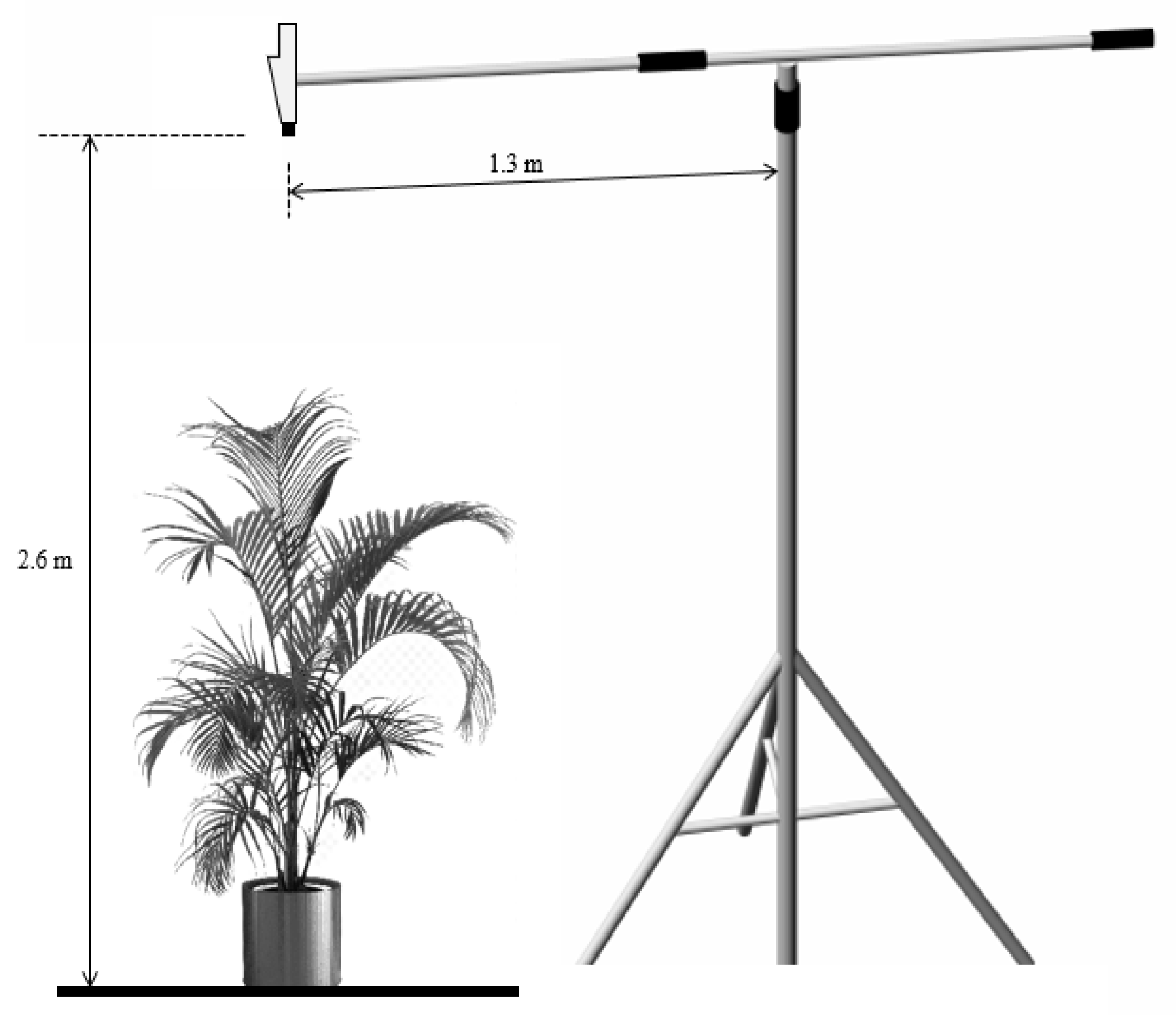
For oil palm seedlings, Shafri et al. [34] acquired reflectance spectra of healthy and G. boninense infected seedlings obtained using APOGEE spectroradiometer (Apogee Instruments Inc., Logan, UT, USA) in three healthiness levels, i.e., healthy, mildly infected, and severely infected. The seedlings were inoculated with G. boninense inoculum at four months old. Reflectance spectra of leaves 1 and 2 were collected after six months of inoculation when disease symptoms appeared for severely infected seedlings. The data were denoised and transformed into the first derivative. The significant bands were identified using a one-way analysis of variance (ANOVA) and were inputted into a maximum likelihood algorithm. The result yielded 82% accuracy with a kappa value of 0.73.

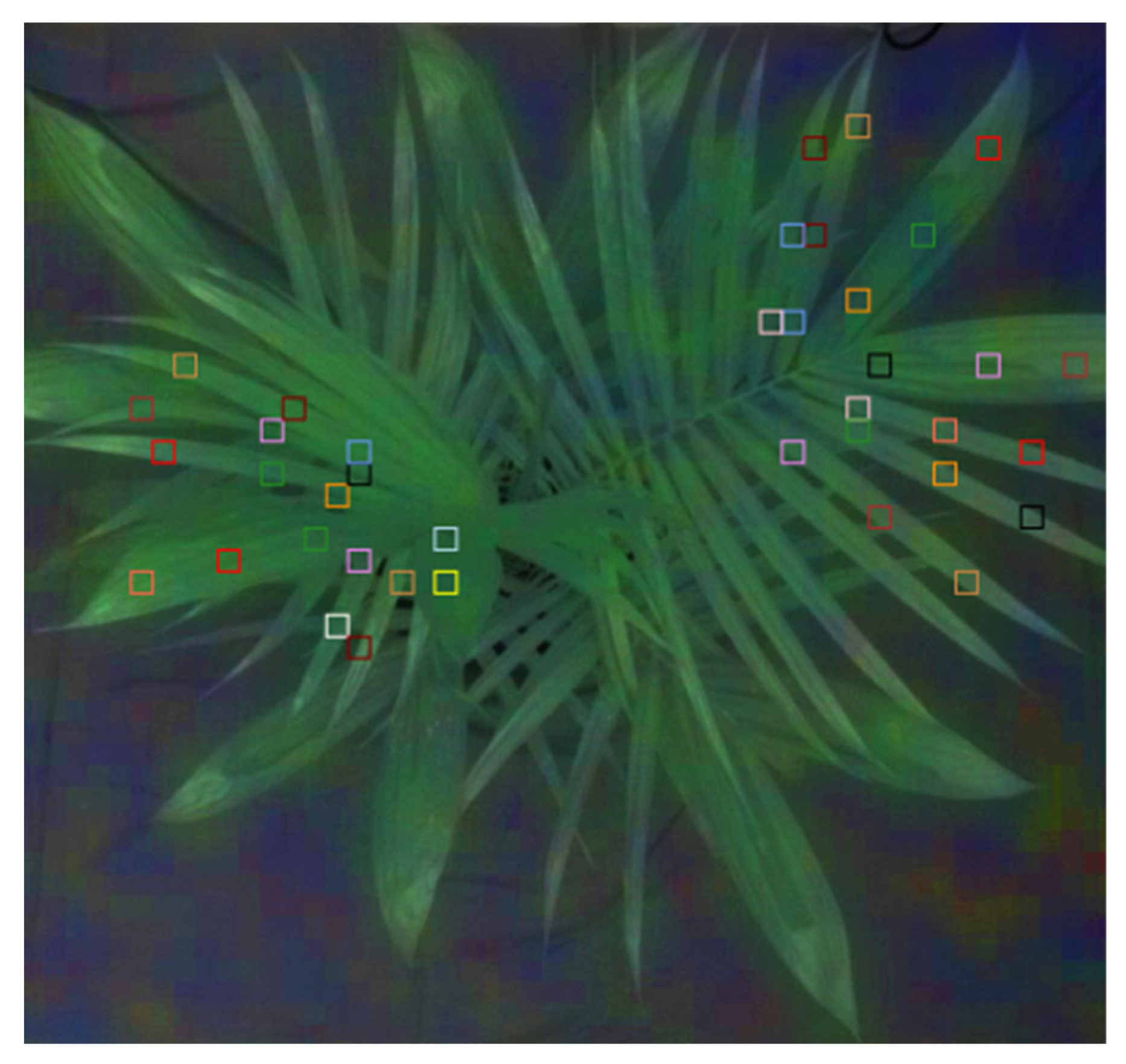
The exploration of hyperspectral imaging and machine learning for G. boninense detection at the seedlings stage was first undertaken by Azmi et al. [35]. The result achieved over 93% classification accuracy in discriminating healthy and asymptomatic G. boninense infected seedlings. However, the limitation of this study was the use of SVM kernel methods such as linear, Gaussian radial basis function (RBF), and polynomial algorithms. On the other hand, this study demonstrated that the combination of reflectance of frond 1 and frond 2 is feasible for early detection of G. boninense infection in oil palm seedlings even before the physical symptoms appear, obviating the need for complex pre-processing to distinguish between those fronds. Additionally, Khairunniza-Bejo et al. [36] utilized a single band of 934 nm to discriminate between healthy and G. boninense-infected oil palm seedlings and discovered the best model to be a linear SVM with a 94.8% accuracy and 0.95 area under the curve. A summary of machine learning application to classify G. boninense infection in oil palm seedlings and mature trees are presented in

Table 1. List of machine learning techniques used for G. boninense detection in oil palm nurseries and plantations.

Study Scale	Applied Sensor	Machine Learning Model	Accuracy (%)	Reference
Nursery	APOGEE spectroradiometer	Maximum likelihood	82	[34]
	FireflEYE S185 hyperspectral camera	SVM kernel functions	100	[35]
	FireflEYE S185 hyperspectral camera	linear SVM	94.8	[36]
Plantation	Intelligent electronic nose (e-nose)	ANN	85	[37]
	Unispec spectroradiometer	PLS-DA	92	[38]
	Unispec spectroradiometer	PLS-DA	94	[28]
	ASD field spectroradiometer	kNN	97	[29]
	FT-IR spectrometer	LDA	92	[30]
	GER 1500 handheld spectrometer	ANN	100	[31]
	Dielectric spectroscopy	QDA	81	[32]
	FARO laser scanner	kernel naïve Bayes	85	[33]

. Different sensors and machine learning models were used to achieve various degrees of classification accuracies. However, studies that utilized hyperspectral reflectance data are limited. Therefore, further study is needed to scrutinize hyperspectral imaging capabilities and machine learning techniques other than SVM to detect G. boninense in oil palm seedlings.

2. Materials and Methods

2.1. Experimental Setup

The study was conducted in the Transgenic Greenhouse, Universiti Putra Malaysia, Serdang, Malaysia. The samples consisted of 28 oil palm seedlings, aged four months old, obtained from Sime Darby Plantation, Banting. The seedling was allowed to adapt to the greenhouse environment for one month prior to artificial inoculation. The temperature and humidity inside the greenhouse were set at 27 °C and 90%, respectively, following the procedure proposed by Oettli et al. [39].

After a month, 15 of the seedlings were inoculated with G. boninense inoculum using techniques described in Naidu et al. [5] and labelled as inoculated (I) seedlings. Meanwhile, the remaining 13 seedlings were served as a control treatment and labelled as uninoculated (U) seedlings. The seedlings were arranged in a standard nursery arrangement, watered, and fertilized sufficiently at the same rate. Two months after the inoculation, two of the I seedlings were sent to Bacteriology Laboratory, Faculty of Agriculture, UPM, Serdang, Malaysia, to confirm the G. boninense infection using a PCR test.

2.2. Data Collection

At five months after inoculation, image acquisition was carried out inside the greenhouse using FireflEYE S185 (Cubert GmbH, Ulm, BW, Germany) hyperspectral snapshot camera. The camera captured 125 bands ranging from 450 nm to 950 nm, including the blue, green, red and near-infrared (NIR) spectrum with a sampling interval of 4 nm. The camera was mounted on a custom tripod and positioned 2.6 m vertically from the ground to obtain the nadir view of the seedlings (Figure 1). The camera was calibrated before each image acquisition with white and dark reference to maintain a similar integration time to minimize the effects of illumination and detector sensitivity. The white calibration was performed by placing the provided white rectangular board (99% light reflection) flat and close to the lens, while the dark calibration was performed by completely closing the camera lens. Thus, each collected image was calibrated as:

$$Reflectance=\frac{\left(Image-Dark\right)}{\left(White-Dark\right)}$$

(1)

The calibrations were tested before image acquisition to ensure a good quality of the output image. One seedling was imaged at a time against a black background board (2 m × 2 m) on a sunny clear day from 11:00 a.m. to 2:00 p.m. local time to maintain a natural illumination. The image acquisition system was controlled by Cube-Pilot software supplemented by the manufacturer.

2.3. Data Pre-Processing

Spectral reflectance was extracted manually and randomly from the first four left and right leaflets (Figure 2) to minimize spectral variations due to the effects of frond inclinations [40]. Twenty sample points were extracted approximately for each seedling, yielding a total of 540 samples for U and 582 samples for I. Thereafter, outliers in the data were removed using the box plot method as suggested in Azmi et al. [35]. Box plot analyzed the data statistically in a graphical manner with five measured parameters representing the distribution, i.e., lower quartile, upper quartile, lower fence, upper fence, and interquartile range. These quartile ranges are advantageous due to their less sensitivity towards outliers [41,42].

2.4. Data Processing

Based on Azmi et al. [35], the detection of G. boninense was determined by analyzing specific spectral signatures of U and I treatments. Only the bands that attained the highest separation between treatments and statistically significant were included for further processing to avoid analytical issues due to unnecessary data. Initially, 35 bands were chosen based on the work of Azmi et al. [35]. Then the number of bands was optimized based on the performance of machine learning classification models. The models were developed using seven machine learning algorithms available in MATLAB’s machine learning toolbox (2019b, The MathWorks Inc., Natick, MA, USA), ran on a personal computer equipped with an Intel^® Core™ i7-8750H processor and 32 GB RAM. Each algorithm is generally described as below:

• Decision trees build classification in the form of a tree structure. The classifier breaks down a dataset into smaller and smaller subsets while at the same time an associated decision tree is incrementally developed. The final result is a tree with decision nodes and leaf nodes. The leaf nodes contain responses in nominal terms such as ‘true’ or ‘false’.
• Discriminant analysis assumes that different classes generate data based on different Gaussian distributions. For example, LDA model has the same covariance matrix for each class with different means, while QDA has both covariances and means of each class different. LDA (Equation (2)) and QDA (Equation (3)) can be expressed as:

  $$\beta =C^{-1}\left({\mu }_1-{\mu }_2\right)$$

  (2)

  where $\beta$ is the linear model coefficients, $C$ is the covariance matrices, and ${\mu }_i$ are the mean vectors.

  $$Z_k\left(x\right)=-\frac{1}{2}{\left(x-{\mu }_k\right)}^T{C}_k^{-1}\left(x-{\mu }_k\right)-\frac{1}{2}ln\left|C_k\right|+lnP\left(C_k\right).$$

  (3)

  where $C_k$ is the covariance matrix for the class $k^{-1}$, $\left|C_k\right|$ is the determinant of the covariance matrix $C_k$, and $P\left(C_k\right)$ is the prior probability of the class $k$.
• Logistic regression predicts the probability of an outcome that can only have two values. The prediction is based on the use of one or several predictors (numerical and categorical). Equation of logistic regression is as below:

  $$l={\log }_b\frac{p}{1-p}={\beta }_0+{\beta }_1{x}_1+{\beta }_2{x}_2$$

  (4)

  where $p=P\left(Y=1\right)$, $b$ is the base of logarithm, ${\beta }_i$ are parameters of the model, and $x_i$ are the predictors.
• Naïve Bayes is a type of probabilistic classifier that discriminates different objects based on specific features. Bayes theorem is represented as:

  $$P\left(A|B\right)=\frac{P\left(B|A\right) P\left(A\right)}{P\left(B\right)}$$

  (5)

  where $A$ and $B$ are events and $P\left(B\right)\ne 0$. $P\left(A|B\right)$ and $P\left(B|A\right)$ are conditional probabilities, and $P\left(A\right)$ and $P\left(B\right)$ are the probabilities of observing $A$ and $B$ independently of each other; this is known as the marginal probability.
• Support Vector Machine (SVM) performs classification by finding the hyperplane that maximizes the margin between the two classes. The vectors (cases) that define the hyperplane are the support vectors. The linear kernel is fit for linearly separable data, which can be expressed as:

  $$k\left(x_i,x_j\right)=x_i^T{x}_j$$

  (6)
• where k is the kernel function, $\left(x_i,x_j\right)$ are a-dimensional input $x_i^T{x}_j$ is a map from a-dimension to b-dimension. An example of non-linear kernels is Gaussian Radial Basis Function (RBF), which can be represented as:

  $$\begin{array}{c}k\left(x_i,x_j\right)=\exp \left(-\frac{{\Vert x_i-x_j\Vert }^2}{2{\sigma }^2}\right)\\ =\exp \left(-\gamma {\Vert x_i-x_j\Vert }^2\right)\end{array}$$

  (7)

  where ${\Vert x_i-x_j\Vert }^2$ is known as the squared Euclidean distance between two feature vectors, and σ is defined as kernel width. Small kernel width tends to reflect dissimilar patterns and cause overfitting, whereas large ones result in very similar patterns and cause underfitting. The optimal kernel width is chosen based on the tradeoff between underfitting and overfitting loss. Besides that, the σ also has a similar definition with kernel scale (γ) where $\gamma =\frac{1}{2{\sigma }^2}$. Another kernel function that was used was polynomial that can be expressed as:

  $$k\left(x_i,x_j\right)={\left(1+x_i^T{x}_j\right)}^p$$

  (8)

  where $p$ is the order of the polynomial kernel. The degree of the polynomial kernel able to influence the tolerance of the classifier resulted in a flexible decision boundary of a higher degree polynomial than the lower one.
• Nearest neighbor is a simple algorithm that stores all available cases and classifies new cases based on similarity measure or distant function. Nearest neighbor is expressed as:

  $$NN=2\overline{d}\sqrt{\frac{n}{a}}$$

  (9)
• where $\overline{d}$ is the average distance between each data, $n$ is the total number of data, and $a$ is the size of the studied area.
• Ensemble modeling meld results from many weak learners into one high-quality ensemble model. Qualities depend on the choice of algorithm. An ensemble classifier is expressed as:

  $$F_T\left(x\right)={\displaystyle \sum }_{t=1}^T{f}_t\left(x\right)$$

  (10)

  where $F_T$ is the model that best fits the training data, and each $f_t$ is a weak learner that takes an object $x$ as input and returns a value that indicates the class of the object.

The total number of samples remaining after removing outliers was 913. This sample was divided into two separate datasets in a 70:30 ratio, with 70% used as input data to develop machine learning classification models, and 30% used as a prediction dataset to test the models’ ability to classify an independent dataset. In MATLAB, the input dataset was automatically divided into two groups, namely training and validation. A five-fold cross-validation technique was used to evaluate the performance of the training model, whereby the dataset was randomly divided into five equal-sized subsamples. Each subsample was used to test the model developed using the other four trained subsamples. This process was repeated five times, with each subsample becoming a testing set once to estimate the model classification skill on unseen data, thus generating a less biased model. The completed models were then subsequently exported and assessed using the prediction dataset. As a result, 23 classification models from various types of kernels, shown in

Table 2. List of classification models and kernel.

Classification Model	Types of Kernels
Decision tree	Fine tree, medium tree, coarse tree
Discriminant analysis	Linear discriminant, quadratic discriminant
Logistic regression	Logistic regression
Naïve Bayes	Gaussian naïve Bayes, kernel naïve Bayes
Support vector machine (SVM)	Linear SVM, quadratic SVM, cubic SVM, fine Gaussian SVM, medium Gaussian SVM, coarse Gaussian SVM,
Nearest neighbor	Fine kNN, medium kNN, coarse kNN, cosine kNN, cubic kNN, weighted kNN,
Ensemble	Bagged trees, subspace discriminant, subspace kNN

, were developed using the identified significant bands.

After the development of classification models, exploratory runs were performed where the 35 significant bands were optimized to find the optimal number of bands that could improve the overall classification accuracy achieved by the models. Considering only 35 significant bands instead of 125 bands can avoid analytical issues due to unnecessary bands, thereby making it less complex and more economical to design future hardware. The optimization process (Figure 3) was carried out with a 50% reduction in the number of significant bands to find the optimum number of bands that could improve the average of all accuracy of machine learning models compared to the previous band, which can be expressed in the equation below:

$$Improvement=n-\left(n-1\right)$$

(11)

where n is the average of all accuracy of the current significant bands and (n−1) is the average of all accuracy of the previous significant bands. However, if the models’ average accuracy did not improve, the number of significant bands was increased by 50%. The optimization process was terminated when the number of bands became greater than 35 or no improvement in the average of all accuracy for at least two previous significant bands. The performance time for each model for each significant band was also recorded in order to assess the models’ capability.

2.5. Assessment of Models Performance

2.5.1. F-Score

After the band optimization and accuracy assessment, the models were further assessed using F-score. Accuracy is an empirical measure that calculates only correct predictions to total predictions (Equation (12)), whereas F-score combines sensitivity and precision into a specific accuracy using an equal weighting for precision and sensitivity [43] as in the equations below:

$$Accuracy=\frac{tp+tn}{tp+fp+tn+fn}$$

(12)

$$Sensitivity=\frac{tp}{tp+fn}=recall$$

(13)

$$Precision=\frac{tp}{tp+fp}$$

(14)

$$F-measure=\frac{\left({\beta }^2+1\right)\times precision\times recall}{{\beta }^2\times precision\times recall}$$

(15)

where $tp$ is a true positive, $tn$ is a true negative, $fp$ is a false positive, and $fn$ is a false negative. Sensitivity is determined by the number of correctly classified examples (true positive) and the number of misclassified examples (false negative). In addition, precision is determined by the number of true positives and examples misclassified as positives (false positive). In the equation, $\beta$ is a parameter that can be tuned to favor precision or sensitivity, where F-score is evenly balanced when $\beta$ = 1. It favors precision over sensitivity when $\beta$ > 1 and vice versa [44].

2.5.2. McNemar’s Test

McNemar’s test is a statistical test for determining the statistical significance of differences in classifier performance. The test is a Chi-square ($x^2$) goodness of fit test that compares the distribution of counts expected under the null hypothesis to the distribution of counts observed. It is applied to a contingency table, with cells containing the number of samples correctly and incorrectly identified, as well as the number of samples correctly classified. The following equation with one degree of freedom is used to calculate the test statistic with continuity correction:

$$x^2=\frac{{\left(\left|b-c\right|-1\right)}^2}{b+c}$$

(16)

where $b$ denotes the number of I seedlings misclassified as U, and $c$ denotes the number of U seedlings misclassified as I. If the $x^2$ at the 95% confidence interval is greater than 3.84, then the p-value is less than 0.05, indicating that the model performs differently in classifying the U and I seedlings.

3. Results

3.1. Reflectance Analysis

Figure 4 shows the average spectral reflectance of U and I seedlings collected at five months after inoculation and standard deviations for each wavelength. Based on the figure, the U seedling established higher reflectance in the green and NIR spectrum at 520 to 570 nm and 750 to 950 nm, respectively. Maximum differences between U and I seedlings were detected in the NIR with values around 12% to 16%. It should also be noted that the NIR reflectance can also distinguish between U and I seedlings without any overlapping wavelength, even though it has higher standard deviations than the green reflectance.

Table 3. The significant bands of leaves reflectance dataset identified by the separation value between U and I reflectance.

Total Significant Bands	Significant Bands (nm)
35	814 818 822 826 830 834 838 842 846 850 854 858 862 866 870 874 878 882 886 890 894 898 902 906 910 914 918 922 926 930 934 938 942 946 950

tabulates 35 significant bands of U and I reflectance spectra based on the work of Azmi et al. [35]. These significant bands accounted for 30% of the 125 bands that were confirmed to be statistically significant. Including only 35 significant bands instead of 125 bands could prevent analytical problems due to excessive bands, which would make the applications in-field less complex, and cost-effective [45].

3.2. Machine Learning Classification

All 35 statistically significant bands tabulated in Table 3 were used as inputs for machine learning classification. The classification output in

Table 4. Classification accuracies obtained by a different number of significant bands.

Classification Model	Classification Accuracy (%)					No. of Attempt with the Highest Accuracy
	Number of Significant Bands
	35	18	9	14	11
Fine tree	92.71	92.87	92.22	91.94	92.36	–
Medium tree	92.63	93.52	93.19	92.59	93.01	–
Coarse tree	94.58	94.81	93.84	93.56	94.49	–
Linear discriminant	90.46	92.92	93.05	92.41	92.73	–
Quadratic discriminant	76.93	88.65	89.39	88.56	91.20	–
Logistic regression	90.73	93.52	91.62	92.77	92.68	–
Gaussian naïve Bayes	94.58	94.58	92.12	93.52	92.45	–
Kernel naïve Bayes	94.81	94.81	92.36	94.49	93.33	–
Linear SVM	94.81	95.23 *	93.33	94.49	94.81	1
Quadratic SVM	93.66	93.24	92.82	93.89	94.72	–
Cubic SVM	94.26	91.62	78.21	88.79	93.56	–
Fine Gaussian SVM	94.81	95.23 *	94.07	94.81	94.07	1
Medium Gaussian SVM	94.81	94.81	93.66	94.81	94.30	–
Coarse Gaussian SVM	94.81	94.81	94.21	93.89	93.89	–
Fine kNN	91.24	91.80	92.12	92.68	92.12	–
Medium kNN	94.81	95.23 *	93.66	94.81	94.39	1
Coarse kNN	94.81	94.81	93.98	94.39	94.30	–
Cosine kNN	92.63	92.96	92.54	92.96	93.28	–
Cubic kNN	94.81	95.23 *	93.65	94.81	94.39	1
Weighted kNN	94.81	95.23 *	94.07	94.49	94.07	1
Bagged trees	94.49	94.26	94.07	94.17	94.17	–
Subspace discriminant	92.36	92.82	92.96	93.47	93.14	–
Subspace kNN	90.85	92.77	92.87	92.68	92.54	–
Average of all accuracy (m)	92.84	93.73	92.35	93.23	93.48
Differences (m − (m − 1))		0.88	−1.38	0.88	0.29
No. of attempt with the highest accuracy	–	5	–	–	–

Note: (*) shows the highest accuracy.

shows that almost all models achieved more than 90% accuracy when using 35 bands. Due to the excellent classification, the number of bands was then reduced by 50%. Next, 18 bands were used as new input for the classification and resulted in 0.88% increases in the average of all accuracy, which means machine learning classification produced higher accuracy when using 18 bands compared to 35 bands. Then, the 18 bands were reduced by 50% to 9 bands. However, the 9 bands produced lower accuracies with an average of 92.36%, indicating decreases of 1.36% compared to 18 bands. Therefore, the 9 bands were subsequently increased by 50% to 14 bands.

The 14 bands have successfully improved the accuracy obtained by 9 bands with 0.88% increases in an average of all accuracy, the same as 35 bands. Since the previous run, the 9 bands have not been able to produce a good performance in machine learning classification; therefore, instead of reducing 14 bands to 7 bands, the process continued by increasing the 7 bands by 50%, i.e., to 11 bands. The results showed that 11 bands generated better classification accuracy than 14 bands, with 0.29% increases in the average of all accuracy. However, the optimization was ended at 11 bands because further reduction will cause a further decrease in classification accuracy, as happened in 9 bands. The list of all significant bands in the optimization process was tabulated in

Table 5. Significant bands that used as inputs of machine learning classifiers.

Total Significant Bands	Significant Bands (nm)
18	826 886 890 894 898 902 906 910 914 918 922 926 930 934 938 942 946 950
9	914 922 926 930 934 938 942 946 950
14	898 902 906 910 914 918 922 926 930 934 938 942 946 950
11	910 914 918 922 926 930 934 938 942 946 950

.

Based on Table 4, it was found that the highest classification accuracy acquired was 95.23%, and only five models earned that accuracy in 18 bands. Further, almost all models of 18 bands obtained similar classification accuracy as 35 bands, and some gained higher accuracy than 35 bands, except for quadratic SVM, cubic SVM, and bagged trees models. A distinct improvement was observed in quadratic discriminant, where the classification accuracy has increased by 11.72%. In comparison, the other models gained an average of 0.6% increase in accuracy except for linear discriminant and subspace kNN that earned around 2% increases.

Furthermore, only quadratic SVM, fine kNN, and subspace discriminant achieved higher accuracy than 18 bands when using 14 bands; however, the increase was only up to 0.88%. The remaining models either had the same classification accuracy as the 18 bands or had a decrease in classification accuracy, with an evident decrease of 2.83% in the cubic SVM model. Nonetheless, fine tree, medium tree, coarse tree, linear discriminant, quadratic discriminant, linear SVM, quadratic SVM, cubic SVM, and bagged trees models of 11 bands outperformed 14 bands in classification accuracy. For instance, cubic SVM obtained 93.56% accuracy at 11 bands compared to 88.79% at 14 bands. Apart from that, two models of 11 bands maintained the same classification accuracy as 14 bands, while the remaining models produced a slightly lower accuracy with an average of 0.43% decrement.

For 9 bands, four models such as a medium tree, linear discriminant, coarse Gaussian SVM, and subspace kNN scored better classification accuracy than 11 bands. Meanwhile, fine Gaussian SVM, fine kNN, and weighted kNN procured equal accuracy as 11 bands, while the other models obtained lower accuracy. A significant decrease was observed in cubic SVM, where the classification accuracy decreased sharply from 93.56% in 11 bands to 78.21% in 9 bands, amounting to a 15.35% decrement.

In short, the 18, 14, and 11 bands have successfully established more accurate machine learning models compared to 35 bands. It was demonstrated by the average of all accuracy tabulated in Table 4, where the 18, 14, and 11 bands attained a higher average than 35 bands, generally indicating that those bands’ models performed better in classifying the I and U seedlings.

F-score was computed and presented in

Table 6. F-score of models developed using the significant bands.

Classification Model	F-Score (%)
	Number of Significant Bands
	35	18	9	14	11
Fine tree	92.93	93.38	92.67	92.81	93.11
Medium tree	92.98	94.08	93.73	93.51	93.81
Coarse tree	95.08	95.45	94.43	94.53	95.11
Linear discriminant	91.50	93.85	94.27	93.59	93.93
Quadratic discriminant	78.23	89.84	90.49	89.90	92.16
Logistic regression	91.33	94.08	92.46	93.73	93.46
Gaussian naïve Bayes	95.08	95.08	92.72	94.08	93.07
Kernel naïve Bayes	95.45	95.45	93.11	95.11	94.16
Linear SVM	95.45	95.77	94.16	95.11	95.45
Quadratic SVM	94.50	94.19	93.89	94.19	95.48
Cubic SVM	94.74	92.46	73.60	90.32	94.53
Fine Gaussian SVM	95.45	95.77	94.81	95.45	94.81
Medium Gaussian SVM	95.45	95.45	94.50	95.45	95.18
Coarse Gaussian SVM	95.45	95.45	95.21	94.87	94.87
Fine kNN	91.58	92.36	92.72	93.46	92.72
Medium kNN	95.45	95.77	94.50	95.45	95.15
Coarse kNN	95.45	95.45	94.84	95.15	95.18
Cosine kNN	92.98	93.33	93.02	93.33	93.69
Cubic kNN	95.45	95.77	94.50	95.45	95.15
Weighted kNN	95.45	95.77	94.81	95.11	94.81
Bagged trees	95.11	94.74	94.81	94.77	94.77
Subspace discriminant	93.11	93.89	94.30	94.57	94.23
Subspace kNN	91.28	93.42	93.38	93.46	93.02

to determine which model was the best. According to the table, the highest F-score was 95.77% when the linear SVM, fine Gaussian SVM, medium kNN, and cubic kNN models were used with 18 bands. Meanwhile, the quadratic SVM model with 11 bands achieved the second-highest F-score of 95.48%. The 35 and 14 bands, on the other hand, obtained the same highest F-score value of 95.45%. The similar models of 35 and 14 bands that attained that accuracy were fine Gaussian SVM, medium Gaussian SVM, medium kNN, and cubic kNN that demonstrated their insensitivity to band optimization. Next, 9 bands obtained 95.21% F-score value only for coarse Gaussian SVM, which was considered the highest for 9 bands.

Due to the fact that a few models achieved the highest F-score, performance time for each model of each band was presented in

Table 7. Performance time of models developed using the significant bands.

Classification Model	Performance Time (s)
	Number of Significant Bands
	35	18	9	14	11
Fine tree	5.0538	4.6277	1.2873	3.6890	3.8240
Medium tree	4.3907	4.2772	0.9609	3.2645	3.3773
Coarse tree	3.9659	4.0446	0.8531	3.0669	3.2237
Linear discriminant	5.5868	3.6876	0.7478	2.7450	2.9791
Quadratic discriminant	5.3982	5.3332	0.6290	4.3591	2.7304
Logistic regression	6.5610	5.1549	1.3870	4.1698	4.3726
Gaussian naïve Bayes	4.4120	4.7064	0.4503	3.7530	3.9366
Kernel naïve Bayes	8.7138	6.6702	2.6167	4.8786	4.6418
Linear SVM	5.1192	4.0248	1.2056	3.5172	3.7279
Quadratic SVM	12.8810	15.0320	15.1990	11.1230	11.6320
Cubic SVM	30.8420	36.4900	33.1880	34.1180	35.0530
Fine Gaussian SVM	6.1060	4.6642	1.0061	3.8789	3.0490
Medium Gaussian SVM	4.8147	4.5799	0.8960	3.7307	2.9310
Coarse Gaussian SVM	5.9675	5.5084	1.7124	4.1013	4.2087
Fine kNN	6.7865	4.9865	0.5287	3.5970	3.7909
Medium kNN	5.7937	4.8772	1.1323	3.9551	3.6686
Coarse kNN	6.1868	5.3351	1.0433	3.8722	4.0413
Cosine kNN	6.0353	5.2496	0.9635	4.3031	3.9559
Cubic kNN	8.9532	6.1620	1.3550	4.8110	5.2101
Weighted kNN	6.4390	5.6440	0.8320	4.7278	4.1607
Bagged trees	11.2750	9.1523	4.2469	8.2750	7.7564
Subspace discriminant	13.2520	9.9335	4.7204	9.0717	8.4402
Subspace kNN	14.1990	10.8960	4.6275	9.4566	9.3989

. Among the models of 35 bands that obtained the highest F-score, medium Gaussian SVM has the shortest performance time of 4.8147 s. Meanwhile, for 18 bands, the shortest performance time of 4.0248 s was attained by linear SVM. For 14 bands, medium Gaussian SVM was developed in 3.7307 s and yielded the same highest F-score as 35 bands; however, 14 bands provided 1.084 s faster performance time. Further, the quadratic SVM of 11 bands took 11.6320 to classify the I and U data, which was the longest time consumed.

It was also discovered that the number of bands and the type of algorithms used affected the model performance; for example, cubic SVM took the longest time to develop a classification model for all bands, with an average of 33.9382 s. Furthermore, when using the 9 bands, Gaussian Nave Bayes provided the shortest performance time of 0.4503 s; however, the F-score was slightly lower than coarse Gaussian SVM by 2.49%. Overall, coarse Gaussian SVM of 9 bands has the shortest performance time of 1.7124 s with an F-score of 95.21%, making it the best model for classifying the I and U seedlings.

Furthermore,

Table 8. P-values of McNemar’s test for each model of each significant bands.

Classification Model	p-Value
	Number of Significant Bands
	35	18	9	14	11
Fine tree	0.0291 *	0.2636	0.1356	0.8312	0.6625
Medium tree	0.0809	0.4795	0.3588	0.8231	1.0000
Coarse tree	0.6056	0.7893	0.6276	0.6276	1.0000
Linear discriminant	0.8445	1.0000	0.2386	0.5023	0.3588
Quadratic discriminant	0.1042	0.7194	0.7103	1.0000	0.8383
Logistic regression	0.1698	0.4795	0.6767	0.3588	0.8231
Gaussian naïve Bayes	0.6056	0.6056	0.2864	0.4795	0.3827
Kernel naïve Bayes	0.7893	0.7893	0.6625	1.0000	0.8137
Linear SVM	0.7893	1.0000	0.8137	1.0000	0.7893
Quadratic SVM	1.0000	0.8137	0.6464	0.8137	0.7893
Cubic SVM	0.4533	0.6767	0.0000 *	0.8551	0.6276
Fine Gaussian SVM	0.7893	1.0000	0.8026	0.7893	0.8026
Medium Gaussian SVM	0.7893	0.7893	1.0000	0.7893	0.6056
Coarse Gaussian SVM	0.7893	0.7893	0.3017	0.4533	0.4533
Fine kNN	0.0455 *	0.2109	0.2864	0.8231	0.2864
Medium kNN	0.7893	1.0000	1.0000	0.7893	1.0000
Coarse kNN	0.7893	0.7893	0.8026	1.0000	0.6056
Cosine kNN	0.0809	0.1175	0.1904	0.1175	0.1687
Cubic kNN	0.7893	1.0000	1.0000	0.7893	1.0000
Weighted kNN	0.7893	1.0000	0.8026	1.0000	0.8026
Bagged trees	1.0000	0.4533	0.8026	0.8026	0.8026
Subspace discriminant	0.6625	0.6464	0.0990	0.3320	0.4795
Subspace kNN	0.0776	0.5023	0.2636	0.8231	0.1904

Note: (*) significant at the p ≤ 0.05.

displayed the p-values of McNemar’s test, which examined only misclassifications of U and I within each model. If the counts of misclassification in U and I are similar or nearly identical, this implies that the models make approximately the same number of errors for both treatments. In this scenario, the result would not be significant, and the null hypothesis would not be rejected. Based on Table 8, nearly all models had p-values greater than 0.05 at the 95% confidence level, implying that there were no significant differences in the misclassification of U and I and that the models were not biased in favor of treatments. In comparison, only three models (fine tree and fine kNN of 35 bands and cubic SVM of 9 bands) obtained the p-values less than 0.05, showing that substantial differences existed in misclassifying the U and I.

4. Discussion

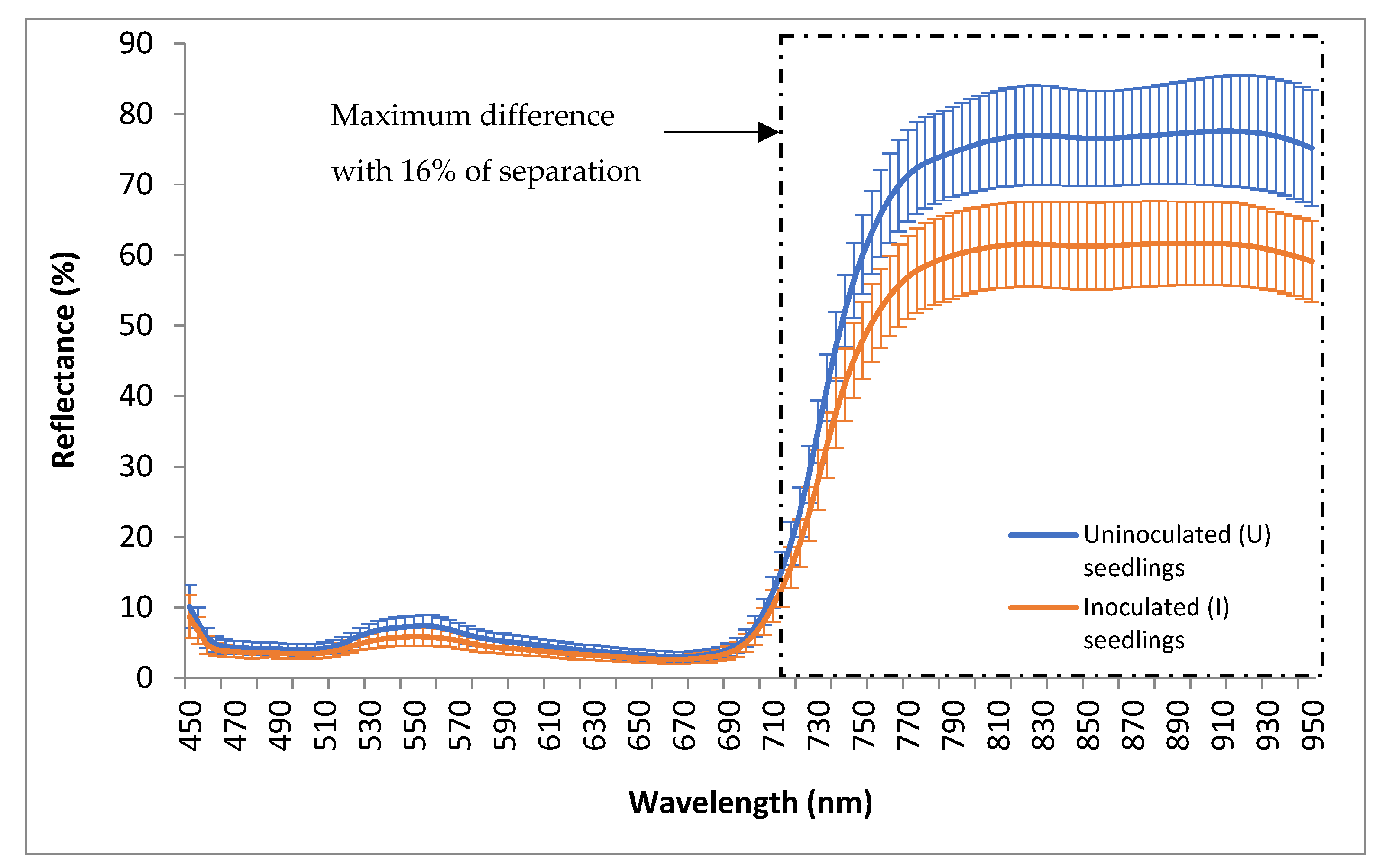
In this study, it should be noted that the low reflectance of the I seedlings in the NIR spectrum was typical for diseased plants that demonstrated the damaged leaf’s internal structure, which consequently causes water stress in the plants. Furthermore, changes in the NIR reflectance during a stress period were more evident than changes in the visible reflectance since NIR could penetrate deeper through the internal leaf structure than visible wavelengths [29]. This finding agreed with [46], where healthy citrus and asymptomatic huanglongbing infected leaves showed significant differences in the NIR spectrum. Undoubtedly, in a nutshell, healthy leaves reflect higher NIR reflectance than infected leaves even before the development of physical symptoms.

Conversely, the U seedlings provide a slightly higher reflectance in the visible spectrum than the I seedlings. This pattern was contrary to the spectral signature of healthy plants examined by other researchers who agreed that healthy plants normally have lower reflectance than a diseased plant in the visible range, especially in green (520 to 560 nm) due to the higher level of chlorophyll in the leaves. However, in this study, the pattern shown was identical to the study carried out by [34], where the healthy seedlings developed higher reflectance than infected seedlings in the green wavelengths. As each plant has a specific spectral signature [47], this pattern may be a unique spectral signature for oil palm seedlings.

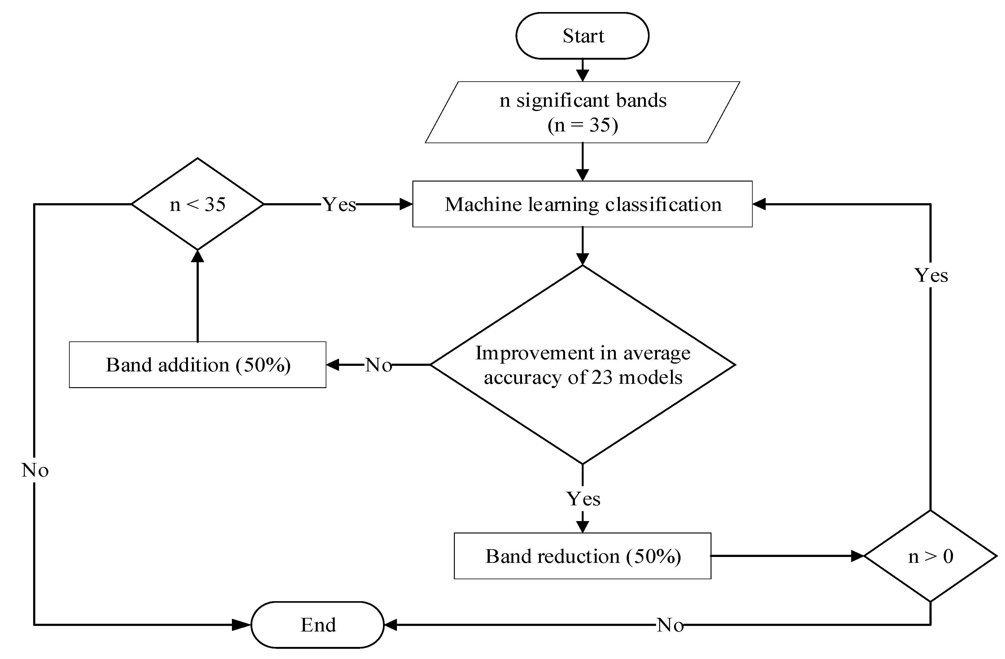
According to [48], a higher number of input parameters in machine learning had resulted in higher accuracy models; however, this finding contrasted with linear discriminant, quadratic discriminant, and subspace kNN models, which produced higher accuracy at a lower number of bands, e.g., 9 bands. In addition, linear SVM has maintained a nearly consistent accuracy of ±95% at 35, 18, 14 and 11 bands despite the reduced number of bands that reflect its insensitivity towards bands optimization. The differences in classification accuracy were due to different characteristics and sensitivities of specific classifiers towards the optimization of parameters [33]. For example, bagged trees only achieved the highest classification accuracy of 94.49% when 35 bands were used, whereas quadratic SVM achieved the highest classification accuracy when 11 bands were used.

Additionally, it was noted that there were minor discrepancies in the percentage classification accuracy and F-score. This is because classification accuracy is only concerned with the total number of correct predictions ($tp$ and $tn$), whereas F-scores balance precision and sensitivity by assigning equal weight to each. Accuracy alone is insufficient as a performance metric for issues involving unequal classification; for example, in this case, U is 279 and I is 360. The key reason for this is that the amount of data of I overwhelmed the amount of data of U, which means that even unskilled models can achieve high classification accuracy, depending on the severity of the class imbalance.

However, the results showed that most SVM-based models achieved a higher F-score than the other models. The linear kernel provided the optimal hyperplane to separate the data points of U and I, followed by the fine and medium gaussian kernels. Additionally, kNN algorithms were also determined as the best classifier based on the classification accuracy obtained, with medium, cubic, and weighted kNN models outperforming other kNN models. Thus, it is revealed that medium distinctions between classes with 10 number of neighbors are more suitable, while one neighbor is too fine, and 100 neighbors are too coarse. On the other hand, the less accuracy from discriminant analysis indicates that the U and I data does not fit with the Gaussian distributions. Furthermore, both classes also do not fit well with the sigmoid function, as indicated by logistic regression results.

Coarse Gaussian SVM is a Gaussian radial basis function (RBF) that was used to improve SVM classification when the data were not linearly separable. The kernel approach enables SVM to find a hyperplane in the kernel space, enabling non-linear separation within the feature space to be viable. The best kernel width is determined by balancing underfitting and overfitting loss. In the remote sensing field, SVM is particularly appealing for managing limited training data effectively and having higher classification accuracy than the conventional classification [49]. The basic principle that benefits SVM compared to conventional classification is the structural risk minimization learning process. SVM minimizes the classification error on unseen data without making prior assumptions about the probability distribution of data [50]. In contrast, conventional classification, such as maximum likelihood, usually assumes that data distribution is a priority.

In recent studies, SVM was frequently used to classify healthily and G. boninense infected oil palm with high accuracy of 100% [35], 94.8% [36], 91% [51], and 89% [32], which confirmed the suitability of SVM classifiers in oil palm disease classification. Furthermore, machine learning classification models typically produced better results compared to conventional classification models, such in the study conducted by Shafri et al. [34] that produced a net accuracy of 82% and kappa coefficient of 0.73 using maximum likelihood to classify multiple severities of G. boninense infection in oil palm seedlings. Furthermore, this finding was not only consistent with previous research conducted for BSR disease in mature oil palm trees, but also with other diseases such as identifying cotton canopy infected with Verticillium wilt, apple scab disease caused by Venturia inaequalis, and corn kernels infected with fungi.

5. Conclusions

In this study, it can be concluded that reflectance spectra of U and I seedlings showed significant differences in the NIR spectrum; therefore, all significant bands were identified from the NIR wavebands. The significant bands were optimized based on the average of all accuracy obtained by the models. For each optimal band (35, 18, 14, 11 and 9 bands), 23 classification models were constructed, e.g., decision trees, discriminant analysis, logistic regression, naïve Bayes, SVM, nearest neighbor, and ensemble modelling. In general, SVM and kNN-based models have been identified as effective classifier algorithms for differentiating between U and I seedlings. However, the coarse Gaussian SVM with 9 bands was determined to be the best model due to the higher F-score and the shorter performance time, demonstrating its potential to attain excellent accuracy even when a small number of bands was used. The main benefit of this study is to assess the capability of machine learning models to detect G. boninense infection at an early stage (asymptomatic). In future studies, the monitoring period of oil palm seedlings could be shortened to less than 10 months to assess the efficacy of hyperspectral imaging to detect G. boninense at the earliest stage of infection.

References

1. Sanderson, F.R. An insight into spore dispersal of Ganoderma boninense on oil palm. Mycopathologia 2005, 159, 139–141. [Google Scholar] [CrossRef] [PubMed]
2. Turner, P.D.; Gillbanks, R.A. Oil Palm Cultivation and Management; Incorporated Society of Planters: Kuala Lumpur, Malaysia, 1974. [Google Scholar]
3. Shu’ud, M.M.; Loonis, P.; Seman, I.A. Towards automatic recognition and grading of Ganoderma infection pattern using fuzzy systems. T. Eng. Comput. Technol. 2007, 19, 51–56. [Google Scholar]
4. Paterson, R.R.M. Ganoderma disease of oil palm—A white rot perspective necessary for integrated control. Crop. Prot. 2007, 26, 1369–1376. [Google Scholar] [CrossRef] [Green Version]
5. Naidu, Y.; Siddiqui, Y.; Rafii, M.Y.; Saud, H.M.; Idris, A.S. Inoculation of oil palm seedlings in Malaysia with white rot hymenomycetes: Assessment of pathogenicity and vegetative growth. Crop Prot. 2018, 110, 146–154. [Google Scholar] [CrossRef]
6. Sariah, M.; Hussin, M.Z.; Miller, R.N.G.; Holderness, M. Pathogenicity of Ganoderma boninense tested by inoculation of oil palm seedlings. Plant Pathol. 1994, 43, 507–510. [Google Scholar] [CrossRef]
7. Idris, A.S.; Kushairi, D.; Ariffin, D.; Basri, M.W. Technique for inoculation of oil palm germinated seeds with Ganoderma. MPOB Inf. Ser. 2006, 314, 1–4. [Google Scholar]
8. Roslan, A.; Idris, A.S. Economic impact of Ganoderma incidence on Malaysian oil palm plantation—A case study in Johor. Oil Palm Ind. Econ. J. 2012, 12, 24–30. [Google Scholar]
9. Meor, M.S.Y.; Khalid, M.A.; Idris, A.S. Identification of basal stem rot disease in local palm oil by microfocus XRF. J. Nucl. Relat. Technol. 2009, 6, 282–287. [Google Scholar]
10. Helmi, Z.; Mohanad, S.E. Quantitative performance of spectral indices in large scale plant health analysis. Am. J. Agric. Biol. Sci. 2009, 4, 187–191. [Google Scholar]
11. Shafri, H.Z.; Hamdan, N. Hyperspectral imagery for mapping disease infection in oil palm plantation using vegetation indices and red-edge techniques. Am. J. Appl. Sci. 2009, 6, 1031. [Google Scholar]
12. Shafri, H.Z.M.; Hamdan, N.; Izzuddin Anuar, M. Detection of stressed oil palms from an airborne sensor using optimized spectral indices. Int. J. Remote Sens. 2012, 33, 4293–4311. [Google Scholar] [CrossRef]
13. Izzuddin, M.A.; Idris, A.S.; Nisfariza, N.M.; Ezzati, B. Spectral based analysis of airborne hyperspectral remote sensing image for detection of Ganoderma disease in oil palm. In Proceedings of the 2015 International Conference on Biological and Environmental Science (BIOES 2015), Phuket, Thailand, 1–2 October 2015; pp. 13–20. [Google Scholar]
14. Izzuddin, M.A.; Nisfariza, M.N.; Ezzati, B.; Idris, A.S.; Steven, M.D.; Boyd, D. Analysis of airborne hyperspectral image using vegetation indices, red edge position and continuum removal for detection of Ganoderma disease in oil palm. J. Oil Palm Res. 2018, 30, 416–428. [Google Scholar]
15. Waibel, A.; Hanazawa, T.; Hinton, G.; Shikano, K.; Lang, K.J. Phoneme recognition using time-delay neural networks. IEEE Trans. Acoust. Speech Signal Process. 1989, 37, 328–339. [Google Scholar] [CrossRef]
16. Baker, J.M.; Deng, L.; Glass, J.; Khudanpur, S.; Lee, C.H.; Morgan, N.; O’Shaughnessy, D. Developments and directions in speech recognition and understanding. IEEE Signal Process. Mag. 2009, 26, 75–80. [Google Scholar] [CrossRef]
17. Friedl, M.A.; Brodley, C.E.; Strahler, A.H. Maximising land cover classification accuracies produced by decision trees at continental to global scales. IEEE Trans. Geosci. Remote Sens. 1999, 37, 969–977. [Google Scholar] [CrossRef]
18. Waske, B.; Van der Linden, S.; Benediktsson, J.A.; Rabe, A.; Hostert, P. Sensitivity of support vector machines to random feature selection in classification of hyperspectral data. IEEE Trans. Geosci. Remote Sens. 2010, 48, 2880–2889. [Google Scholar] [CrossRef] [Green Version]
19. Su, Y.X.; Xu, H.; Yan, L.J. Support vector machine-based open crop model (SBOCM): Case of rice production in China. Saudi J. Bio. Sci. 2017, 24, 537–547. [Google Scholar] [CrossRef] [PubMed]
20. Ferentinos, K.P. Deep learning models for plant disease detection and diagnosis. Comput. Electron. Agric. 2018, 145, 311–318. [Google Scholar] [CrossRef]
21. Pantazi, X.E.; Tamouridou, A.A.; Alexandridis, T.K.; Lagopodi, A.L.; Kontouris, G.; Moshou, D. Detection of Silybum marianum infection with Microbotryum silybum using VNIR field spectroscopy. Comput. Electron. Agric. 2017, 137, 130–137. [Google Scholar] [CrossRef]
22. Hu, H.; Pan, L.; Sun, K.; Tu, S.; Sun, Y.; Wei, Y.; Tu, K. Differentiation of deciduous-calyx and persistent-calyx pears using hyperspectral reflectance imaging and multivariate analysis. Comput. Electron. Agric. 2017, 137, 150–156. [Google Scholar] [CrossRef]
23. Grinblat, G.L.; Uzal, L.C.; Larese, M.G.; Granitto, P.M. Deep learning for plant identification using vein morphological patterns. Comput. Electron. Agric. 2016, 127, 418–424. [Google Scholar] [CrossRef] [Green Version]
24. Matthews, S.G.; Miller, A.L.; PlÖtz, T.; Kyriazakis, I. Automated tracking to measure behavioral changes in pigs for health and welfare monitoring. Sci. Rep. 2017, 7, 17582. [Google Scholar] [CrossRef] [PubMed]
25. Morales, I.R.; Cebrián, D.R.; Blanco, E.F.; Sierra, A.P. Early warning in egg production curves from commercial hens: An SVM approach. Comput. Electron. Agric. 2016, 121, 169–179. [Google Scholar] [CrossRef]
26. Feng, Y.; Peng, Y.; Cui, N.; Gong, D.; Zhang, K. Modelling reference evapotranspiration using extreme learning machine and generalized regression neural network only with temperature data. Comput. Electron. Agric. 2017, 136, 71–78. [Google Scholar] [CrossRef]
27. Morellos, A.; Pantazi, X.E.; Moshou, D.; Alexandridis, T.; Whetton, R.; Tziotzios, G.; Mouazen, A.M. Machine learning based prediction of soil total nitrogen, organic carbon and moisture content by using VIS-NIR spectroscopy. Biosyst. Eng. 2016, 152, 104–116. [Google Scholar] [CrossRef] [Green Version]
28. Lelong, C.C.; Roger, J.M.; Brégand, S.; Dubertret, F.; Lanore, M.; Sitorus, N.A.; Caliman, J.P. Evaluation of oil-palm fungal disease infestation with canopy hyperspectral reflectance data. Sensors 2010, 10, 734–747. [Google Scholar] [CrossRef]
29. Liaghat, S.; Ehsani, R.; Mansor, S.; Shafri, H.Z.; Meon, S.; Sankaran, S.; Azam, S.H. Early detection of basal stem rot disease (Ganoderma) in oil palms based on hyperspectral reflectance data using pattern recognition algorithms. Int. J. Remote Sens. 2014, 35, 3427–3439. [Google Scholar] [CrossRef]
30. Liaghat, S.; Mansor, S.; Ehsani, R.; Shafri, H.Z.M.; Meon, S.; Sankaran, S. Mid-infrared spectroscopy for early detection of basal stem rot disease in oil palm. Comput. Electron. Agric. 2014, 101, 48–54. [Google Scholar] [CrossRef]
31. Ahmadi, P.; Muharam, F.M.; Ahmad, K.; Mansor, S.; Abu Seman, I. Early detection of Ganoderma basal stem rot of oil palms using artificial neural network spectral analysis. Plant Dis. 2017, 101, 1009–1016. [Google Scholar] [CrossRef] [PubMed] [Green Version]
32. Khaled, A.Y.; Abd Aziz, S.; Bejo, S.K.; Nawi, N.M.; Seman, I.A. Spectral features selection and classification of oil palm leaves infected by basal stem rot (BSR) disease using dielectric spectroscopy. Comput. Electron. Agric. 2018, 144, 297–309. [Google Scholar] [CrossRef]
33. Husin, N.A.; Khairunniza-Bejo, S.; Abdullah, A.F.; Kassim, M.S.; Ahmad, D.; Azmi, A.N. Application of ground-based LiDAR for analyzing oil palm canopy properties on the occurrence of basal stem rot (BSR) Disease. Sci. Rep. 2020, 10, 6464. [Google Scholar] [CrossRef] [PubMed] [Green Version]
34. Shafri, H.Z.; Anuar, M.I.; Seman, I.A.; Noor, N.M. Spectral discrimination of healthy and Ganoderma-infected oil palms from hyperspectral data. Int. J. Remote Sens. 2011, 32, 7111–7129. [Google Scholar] [CrossRef]
35. Azmi, A.N.N.; Bejo, S.K.; Jahari, M.; Muharam, F.M.; Yule, I.; Husin, N.A. Early detection of Ganoderma boninense in oil palm seedlings using support vector machines. Remote Sens. 2020, 12, 3920. [Google Scholar] [CrossRef]
36. Khairunniza-Bejo, S.; Shahibullah, M.S.; Azmi, A.N.N.; Jahari, M. Non-destructive detection of asymptomatic Ganoderma boninense infection of oil palm seedlings using NIR-hyperspectral data and support vector machine. Appl. Sci. 2021, 11, 10878. [Google Scholar] [CrossRef]
37. Abdullah, A.H.; Adom, A.H.; Ahmad, M.N.; Saad, M.A.; Tan, E.S.; Fikri, N.A.; Zakaria, A. Electronic nose system for Ganoderma detection. Sens. Lett. 2011, 9, 353–358. [Google Scholar] [CrossRef]
38. Lelong, C.C.; Roger, J.M.; Bregand, S.; Dubertret, F.; Lanore, M.; Sitorus, N.A.; Caliman, J.P. Discrimination of fungal disease infestation in oil-palm canopy hyperspectral reflectance data. In Proceedings of the First Workshop on Hyperspectral Image and Signal Processing: Evolution in Remote Sensing, Grenoble, France, 26–28 August 2009; IEEE: New York, NY, USA, 2009. [Google Scholar]
39. Oettli, P.; Behera, S.K.; Yamagata, T. Climate based predictability of oil palm tree yield in Malaysia. Sci. Rep. 2018, 8, 2271. [Google Scholar] [CrossRef] [PubMed] [Green Version]
40. Asaari, M.S.M.; Mishra, P.; Mertens, S.; Dhondt, S.; Inzé, D.; Wuyts, N.; Scheunders, P. Close-range hyperspectral image analysis for the early detection of stress responses in individual plants in a high-throughput phenotyping platform. ISPRS J. Photogramm. Remote Sens. 2018, 138, 121–138. [Google Scholar] [CrossRef]
41. Wilcox, R.R. A fundamental problem. In Fundamentals of Modern Statistical Methods: Substantially Improving Power and Accuracy, 2nd ed.; Springer: New York, NY, USA, 2010; pp. 109–126. [Google Scholar]
42. Kwak, S.K.; Kim, J.H. Statistical data preparation: Management of missing values and outliers. Korean J. Anesthesiol. 2017, 70, 407. [Google Scholar] [CrossRef]
43. Sokolova, M.; Japkowicz, N.; Szpakowicz, S. Beyond accuracy, F-score and ROC: A family of discriminant measures for performance evaluation. In Proceedings of the Australasian Joint Conference on Artificial Intelligence, Hobart, Australia, 4–8 December 2006; Springer: Berlin/Heidelberg, Germany, 2006. [Google Scholar]
44. Joshi, P.P.; Wynne, R.H.; Thomas, V.A. Cloud detection algorithm using SVM with SWIR2 and tasseled cap applied to Landsat 8. Int. J. Appl. Earth Obs. Geoinf. 2019, 82, 101898. [Google Scholar] [CrossRef]
45. Wang, Q.; Li, Q.; Li, X. Hyperspectral band selection via adaptive subspace partition strategy. IEEE J. Sel. Top. Appl. Earth Obs. Remote Sens. 2019, 12, 4940–4950. [Google Scholar] [CrossRef]
46. Deng, X.; Huang, Z.; Zheng, Z.; Lan, Y.; Dai, F. Field detection and classification of citrus Huanglongbing based on hyperspectral reflectance. Comput. Electron. Agric. 2019, 167, 105006. [Google Scholar] [CrossRef]
47. Schweiger, A.K.; Schütz, M.; Risch, A.C.; Kneubühler, M.; Haller, R.; Schaepman, M.E. How to predict plant functional types using imaging spectroscopy: Linking vegetation community traits, plant functional types and spectral response. Methods Ecol. Evol. 2017, 8, 86–95. [Google Scholar] [CrossRef]
48. Zhang, Y.; Ling, C. A strategy to apply machine learning to small datasets in materials science. Npj Comput. Mater. 2018, 4, 25. [Google Scholar] [CrossRef] [Green Version]
49. Savas, C.; Dovis, F. Comparative performance study of linear and gaussian kernel SVM implementations for phase scintillation detection. In Proceedings of the 2019 International Conference on Localization and GNSS (ICL-GNSS), Nuremberg, Germany, 1–6 June 2019. [Google Scholar]
50. Faris, H.; Hassonah, M.A.; Ala’M, A.Z.; Mirjalili, S.; Aljarah, I. A multi-verse optimizer approach for feature selection and optimizing SVM parameters based on a robust system architecture. Neural Comput. Appl. 2018, 30, 2355–2369. [Google Scholar] [CrossRef]
51. Kresnawaty, I.; Mulyatni, A.S.; Eris, D.D.; Prakoso, H.T.; Triyana, K.; Widiastuti, H. Electronic nose for early detection of basal stem rot caused by Ganoderma in oil palm. IOP Conf. Ser. Earth Environ. Sci. 2020, 468, 012029. [Google Scholar] [CrossRef]
Figure 1. Illustration of image acquisition setup inside the greenhouse.
Applsci 11 11798 g001
Figure 2. Spectral extraction using Cube-Pilot of left and right leaflets.
Applsci 11 11798 g002
Figure 3. Flowchart of the optimization process of significant bands.
Applsci 11 11798 g003
Figure 4. Spectral reflectance at U and I treatments. Each value represents a mean of 540 and 582 sample points of U and I, respectively. Vertical bars represent standard deviation.
Applsci 11 11798 g004