
Stochastic Model-Predictive Control with Uncertainty Estimation for Autonomous Driving at Uncontrolled Intersections


Department of Mechanical and Automotive Engineering, Seoul National University of Science and Technology, Seoul 01811, Korea
Appl. Sci. 2021, 11(20), 9397; https://doi.org/10.3390/app11209397
Submission received: 16 September 2021
/
Revised: 5 October 2021
/
Accepted: 9 October 2021
/
Published: 10 October 2021
(This article belongs to the Special Issue The Development and Prospects of Autonomous Driving Technology)
Abstract
:This paper presents an uncontrolled intersection-passing algorithm with an integrated approach of stochastic model-predictive control and prediction uncertainty estimation for autonomous vehicles. The proposed algorithm is designed to utilize information from sensors mounted on the autonomous vehicle and high-definition intersection maps. The proposed algorithm is composed of two modules, namely target state prediction and a motion planner. The target state prediction module has predicted the future behavior of intersection-approaching vehicles based on human driving data. The recursive covariance estimator has been utilized to estimate the prediction uncertainty for each approaching vehicle. The desired driving mode has been determined based on the uncontrolled intersection theory. The estimated prediction uncertainty has been used to define the probability distribution of the stochastic model-predictive controller to cope with time-varying uncertainty characteristics of the perception algorithm. The constrained stochastic model-predictive controller based on safety indexes has determined the desired longitudinal acceleration. The proposed robust intersection-passing algorithm has been evaluated via computer simulation based on Monte Carlo simulation with a sensor model. The simulation results showed that the proposed algorithm guarantees the minimum safety constraints and improves the ride comfort at uncontrolled intersections by estimating the uncertainty of sensors and prediction.
1. Introduction
Autonomous or self-driving vehicles are attracting attention as a solution for transportation due to their various advantages such as improved safety, increased traffic efficiency, decrease in pollution, and equitable access to mobility. The coverage of autonomous driving has been extended from the motorway to urban roads to spread these advantages. In this process, uncontrolled intersections are one of the most dangerous driving situations because there is no traffic signal to control the traffic participants. In particular, the accident rate and fatality rate at uncontrolled intersections are higher than in other driving environments [1,2]. Several studies tried to figure out the important factors related to the geometric and traffic-related elements that affect the accident rates of intersections [3,4]. Based on the achievements of accident analysis in intersections, situation awareness, decision making, and motion planning become important issues to pass an uncontrolled intersection safely and comfortably. Various algorithms have been proposed for autonomous driving at uncontrolled intersections.
Various approaches have been used for decision making and motion planning for uncontrolled intersections. In many previous studies, decision making at intersections has been designed based on pre-defined policies. The Markov Decision Process (MDP) has been utilized as a policy-based motion planning algorithm. In particular, the partially observable Markov decision process was introduced to overcome the limitations of unmeasurable variables from the sensors and communication [5,6,7,8]. In these studies, the uncertainty of the surrounding vehicles was considered at the maneuver level, which affects the driving policy decisions of the autonomous vehicles. The Bayesian network was also utilized for probabilistic decision making at intersections. A time window for observation was considered to improve the performance of the Bayesian network [9]. The rule-based approach was applied to select the optimal rule from the pre-defined rule sets [10]. The MDP and the deep Q-network algorithm were established to obtain the optimal driving policy based on traffic image analysis using convolution neural networks [11].
In addition to the decision-making problem, there have been studies focused on determining the driving path and acceleration command for the autonomous vehicle. The combined approach of Gaussian processes regression and a rapidly exploring random tree was used to generate a desired local path to guide the autonomous vehicle through the intersection [12]. The robust Model Predictive Control (MPC) was used for optimal velocity planning under the assumption that all target information is available [13]. The loosely coupled low-complexity MPC was formulated for automated yield maneuvers [14]. The linear MPC with target vehicle motion prediction and driving mode decision was employed to achieve human-like behavior at uncontrolled intersections [15]. In addition, the cooperative scheduling method of all intersection-approaching vehicles was proposed under the assumption of a connected autonomous vehicle [16,17,18,19]. In particular, virtual platooning was introduced, in which vehicles traveling on each branch are transferred to the same road [17].
In order to improve the performance of the decision-making and motion-planning algorithm, various studies have been conducted on traffic modeling and predictions on surrounding vehicles at intersections. The prediction can be classified as maneuver-level [5,6,7,8,19,20] and trajectory-level prediction [9,21] based on the output of the predictor. A game theory was used to model the vehicle interactions in unsignalized intersections [20]. The map-based prediction was used to provide the lane-level prediction results [9]. A learning-based approach, such as the support vector machine and the long short-term memory-based recurrent neural network [21,22], was also utilized to predict the future behavior of surrounding vehicles. However, predictions based on the perception results inevitably have uncertainties in perception information. Many studies have assumed that Vehicle to Vehicle (V2V) can provide the true values of target states without uncertainty [10,16,17,18,19,23,24].
According to a careful review of the previous studies, various approaches have been introduced to develop the prediction and motion-planning algorithm for intersections. Many studies focused on the maneuver decision of the autonomous vehicle among the pre-defined policies. In particular, MDP-based approaches were frequently utilized to select the optimal policy. However, the computational burden of MDP is an obstacle to achieving real-time implementation. MPC was also employed to calculate the desired acceleration to pass the intersection. When using MPC, the target states were often provided by V2V communication to overcome the limitations of perception caused by blind spots and sensor uncertainty. A robust motion planner that can manage the perception and prediction uncertainty has not been addressed much in previous studies.
In this paper, the motion planner based on SMPC with prediction uncertainty estimation is proposed and evaluated. The objectives of the proposed algorithm are ensuring safety, robustness to sensor uncertainty, and minimizing control efforts. Prediction uncertainty of the prediction algorithm is estimated using the recursive covariance estimator to improve the Intelligent Driver Model (IDM)-based prediction algorithm. The estimated uncertainty is used to define the probability distribution of the chance constraint for the SMPC problem, which improves the performance under changes in sensor noise. The desired longitudinal acceleration is decided by solving the SMPC problem. The proposed algorithm has been evaluated via computer simulation using MATLAB/Simulink and FORCES solver.
2. Overall Architecture of Proposed Algorithm
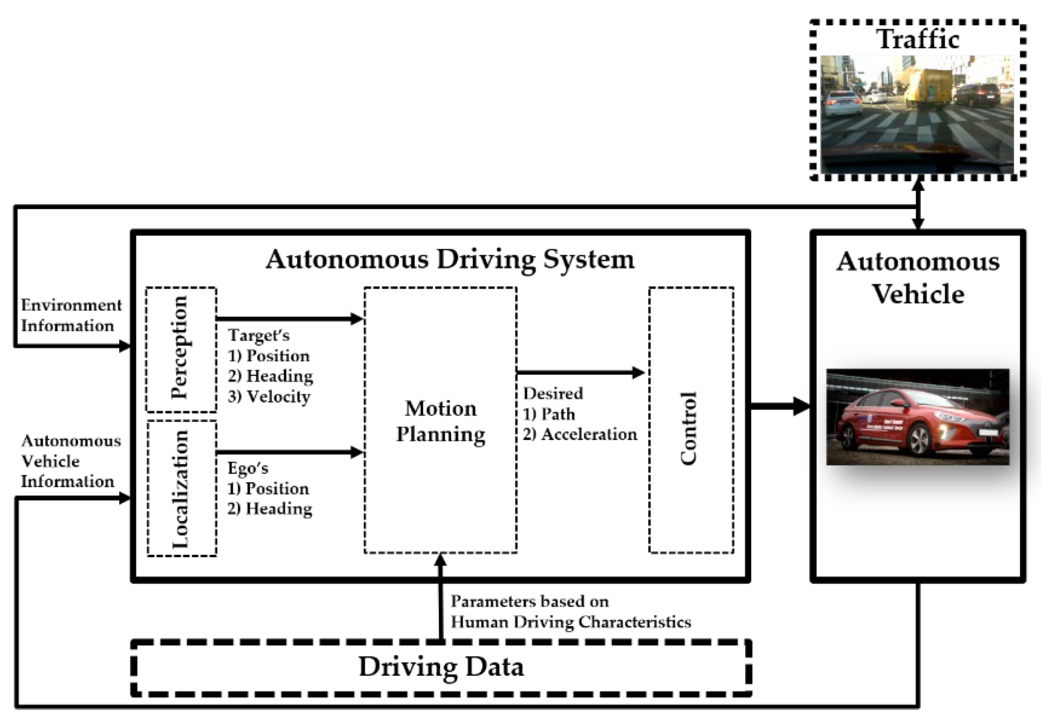
The core functions of autonomous driving can be categorized into four categories, namely perception, localization, motion planning, and control, with the interactions between the autonomous vehicle and the environments depicted in Figure 1. The perception module has a role to detect the surrounding objects around the autonomous vehicle. In this study, a geometric model-free approach [25] has been used to process the LiDAR point clouds from the six IBEO Lux sensors. This algorithm provides the local position, heading angle, and velocity of the moving objects with a grid-base static obstacle map. The localization module estimates the current global position and heading angle of the autonomous vehicle with respect to the high-definition map. A map-matching algorithm with a multi-rate Kalman filter has been used based on the measurement of GPS/INS sensors, LiDAR, and an around-view camera. The control module determines the steering-wheel angle, throttle, and brake inputs to track the desired path and acceleration.
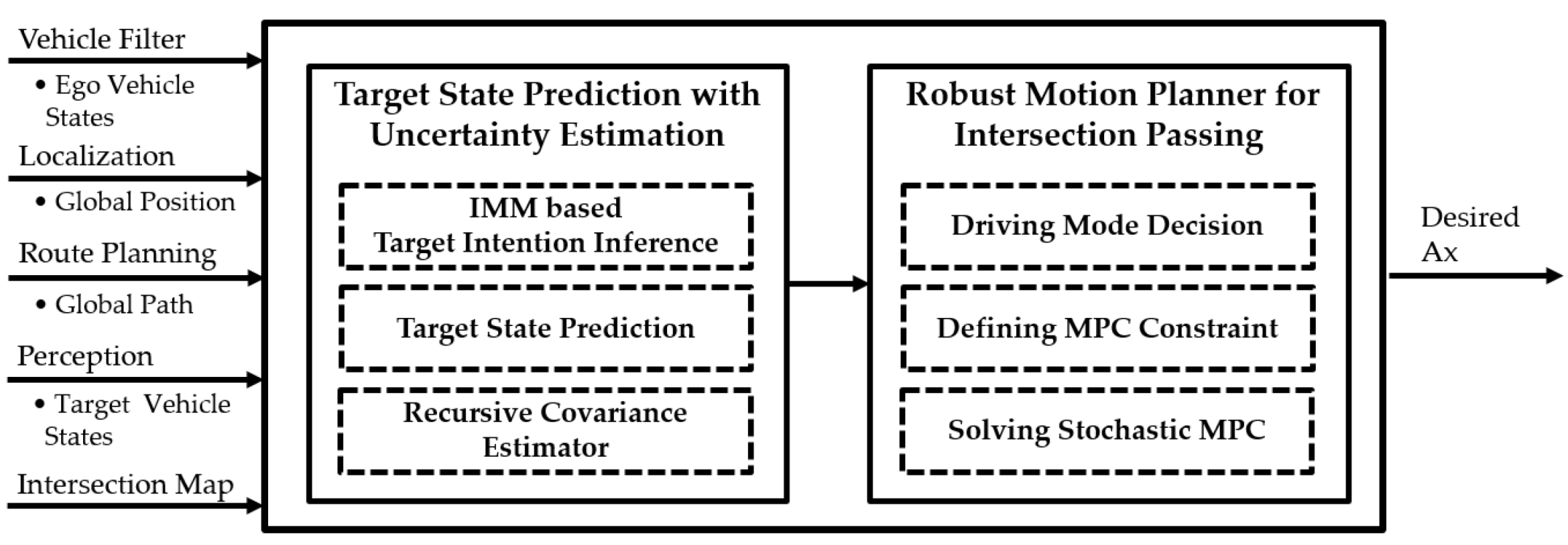
The last module, motion planning, is mainly discussed in this article. The architecture of the proposed motion-planning algorithm for an uncontrolled intersection is shown in Figure 2. The motion-planning algorithm consists of two parts with three sub-modules. The first part, target state prediction with uncertainty estimation, is composed of the three sub-modules intention inference, state prediction, and the recursive covariance estimator. These modules have been utilized to predict the future trajectory of the approaching targets and estimate the prediction uncertainty based on the result of driving intention inference and a recursive covariance estimator. The second part, the robust motion planner for intersection passing, consists of the three sub-modules driving mode decision, defining MPC constraint decision, and solving SMPC. The driving mode of the autonomous vehicle has been determined among ‘Cross’, ‘Yield’, and ‘Stop’ modes according to the uncontrolled intersection theory. Depending on the driving mode, predicted states of the target, and estimated prediction uncertainty, the hard and chance constraints for the SMPC problem have been defined to satisfy the safety index thresholds, which are derived from the human driving data. Finally, the desired acceleration is calculated by the SMPC.
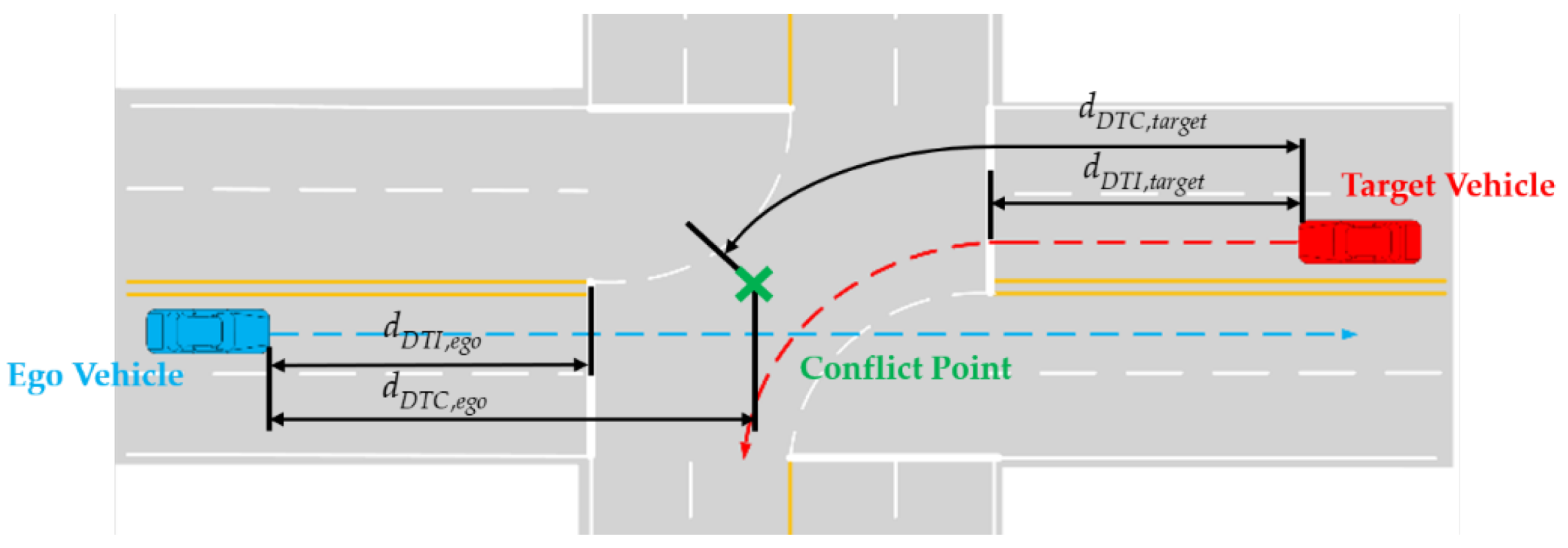
Before proceeding further with the discussion in this paper, the safety indexes for the intersection scenario have been defined as shown in Figure 3. From both a safety and performance perspective, the clearance and time to collision (TTC) have been widely used as an important index for the research of advanced driving-assistant systems (ADAS) and autonomous vehicles. However, the driving situation of an intersection is quite different from nominal driving conditions. Therefore, the clearance and TTC have been modified to consider the conflict point between intersection-approaching vehicles as follows:
where ‘conf’ and ‘DTC’ are the abbreviation of ‘conflict point’ and ‘distance to conflict point’. dDTC,ego and dDTC,target represent the remaining distance to the conflict point of ego and the target vehicle. vego and vtarget are the velocity of the ego and target vehicle, respectively. In addition, the proposed safety index considers the trade-off of cross priority between two vehicles encountered at an intersection. The trade-off relationship of each term in TTCconf applies equally to Cconf. Therefore, Cconf and TTCconf is the suitable safety index that can be utilized for all driving situations. In addition, the remaining distance to the stop line of the intersection is denoted as dDTI, where ‘DTI’ means the distance to the intersection. dDTI is used to depict an evaluation result in the distance domain.
3. Target State Prediction with Uncertainty Estimation
The state prediction of the surrounding objects is generally used in autonomous driving research for motion planners because autonomous vehicles should act like human drivers, who have intuition to be aware of the driving situation. In this research, the objective of state prediction is to provide the information for the driving mode and desired acceleration decision, which are robust to sensor and prediction uncertainty. Therefore, the prediction algorithm has the rule to infer the driving intention and predict the future states of the intersection-approaching vehicles with uncertainty prediction.
3.1. Intention Inference and State Prediction
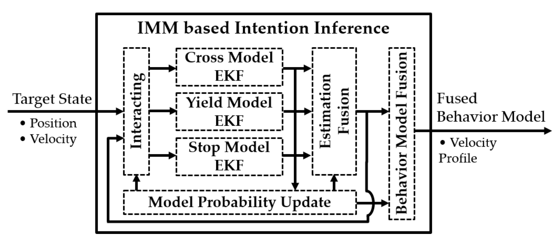
Because the behavior of the approaching vehicles can vary widely, it is difficult to express the future behavior with a few models without compromising the continuity of behavior. However, if too many models are used to overcome this problem, the computational load becomes too burdensome to achieve real-time performance. This study utilized the interacting multiple model (IMM) filter to estimate the probability of each behavior model, which is used to fuse each behavior model. A block diagram of the proposed IMM-based target intention inference algorithm is described in Figure 4. The purpose of the IMM filter is to define the fused behavior model by integrating the behavior model of the local extended Kalman filter (EKF) based on probability.
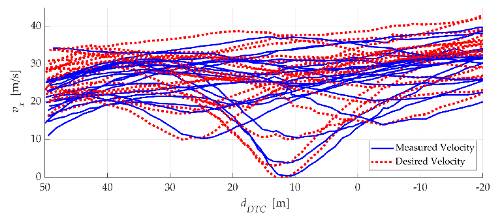
The first step of designing the IMM filter is defining the behavior model for local EKF. The ‘Cross’, ‘Yield’, and ‘Stop’ models are defined based on the collected driving data. The data were collected at Midan City, Incheon, South Korea. The velocity profiles of the collected driving data are described in Figure 5. As shown in Figure 5, am asymmetric characteristic of the acceleration usage has been observed, which is biased to braking. Therefore, the IDM has been selected to model the asymmetric acceleration profile [26]. The IDM is composed of two terms, namely the desired velocity tracking term and the car-following behavior term, as follows:
where amax is the maximum acceleration. v and vdes are the vehicle velocity and desired velocity. s, s*, and Δv are the clearance, desired clearance, and relative velocity to the preceding vehicle. Parameters T, b, and δ are the desired time headway, comfortable braking deceleration, and acceleration exponent.
The collected velocity profiles should be converted to the desired velocity profiles to use the IDM as a process update model of the local EKF. The desired velocity tracking term of the IDM has been rearranged to calculate vdes from the v profile. The rearranged IDM is as follows:
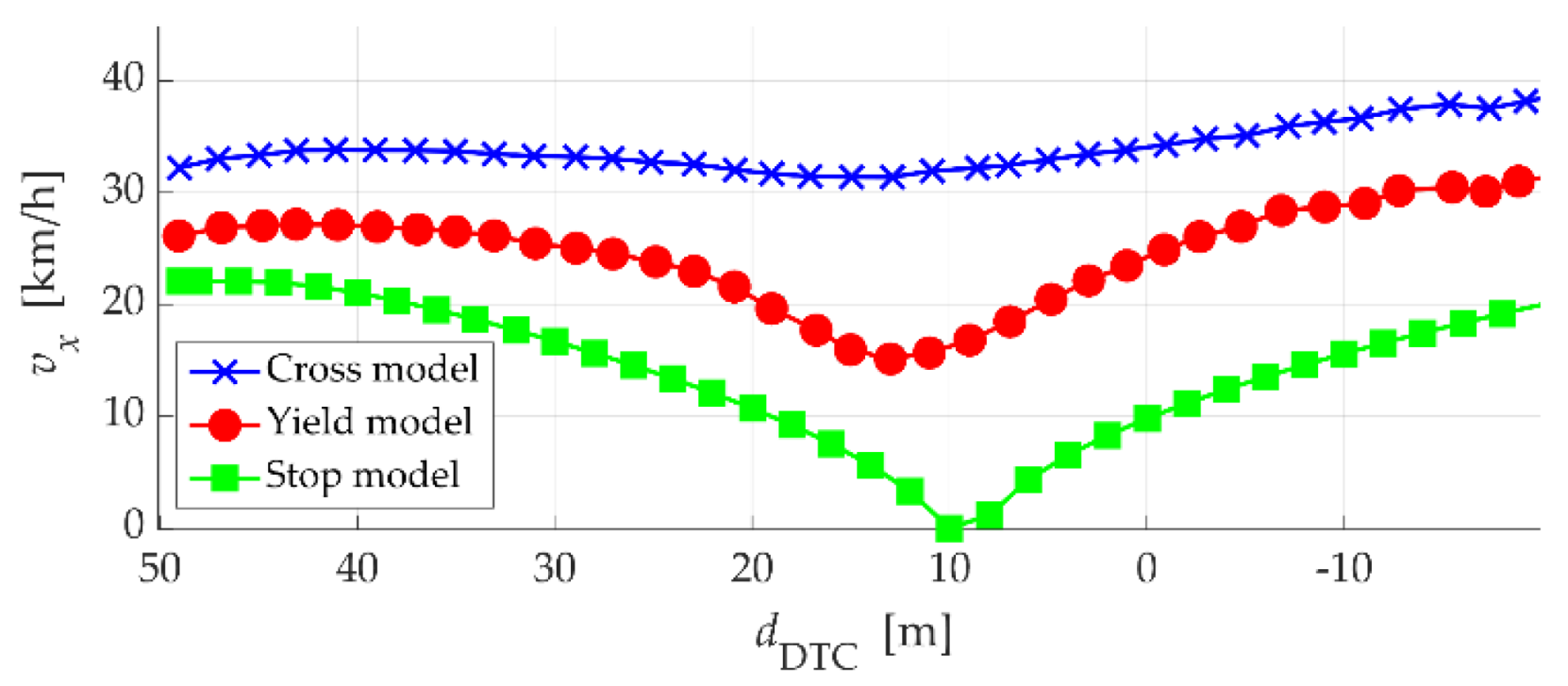
where i is the data index of each profile. The generated desired velocity profiles are presented in Figure 5 as a red dotted line. Parameters amax of 5.0 m/s2 and δ of 4 have been used to calculate the vdes,i(s). The derived vdes,i(s) profiles have been clustered by K-means clustering to define the behavior model as depicted in Figure 6. As mentioned before, these three vdes,i(s) profiles have been named ‘Cross’, ‘Yield’, and ‘Stop’ models and used to determine the process update model of local EKF.
The local filters have been designed as an IDM-based EKF to use ‘Cross’, ‘Yield’, and ‘Stop’ models. The state vector x and measurement vector z of the IDM-based EKF has been defined as follows:
where p, v, and a are the dDTC, velocity, and acceleration, respectively. Parameters pmeas and vmeas represent the measurement of the dDTC and velocity from the sensor of the autonomous vehicle. The process update of IDM-based EKF is defined as follows:
where the parameters dt of 0.1 s and τx of 0.5 s are the sampling time and acceleration delay constant of the IDM-based EKF. The probabilities of each local filter are estimated by using the probability update process of the IMM filter. First, the mixing probability of the i-th model is calculated as follows:
where cj is the normalizing factor and μi is the i-th model probability. pij is the transition probability from the i-th model to the j-th model under the assumption of the Markov chain. The mixed state is calculated as follows:
Based on the mixed state, filtering using the IDM-based EKF is performed. The model probability is updated with the likelihood ratio Λj,k as follows:
In Equation (9), rj,k is the residual of the j-th model, and Sj,k is the covariance matrix of the residual. The remaining parts and details of the IMM filter can be found in [27].
The process update of each IDM-based EKF has been conducted within the prediction horizon to predict the future states of the target vehicle. In this study, the fused behavior model has been derived by using the individual behavior model based on the estimated probability of each model. Therefore, the desired velocity profile of the fused behavior model has been defined as follows:
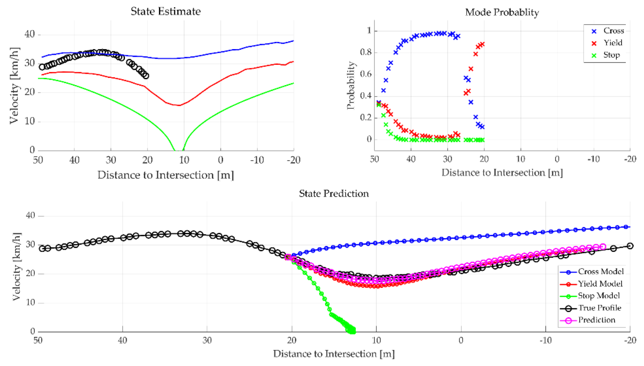
The fused behavior model, vdes,fused(s), has been used as a desired velocity profile of the IDM to predict the future state of the target vehicle based on the sensor measurements. The example of state prediction with an estimated probability is summarized in Figure 7. As shown in Figure 7, the proposed predictor provides more accurate prediction results than the single model prediction case.
3.2. Recursive Uncertainty Estimation
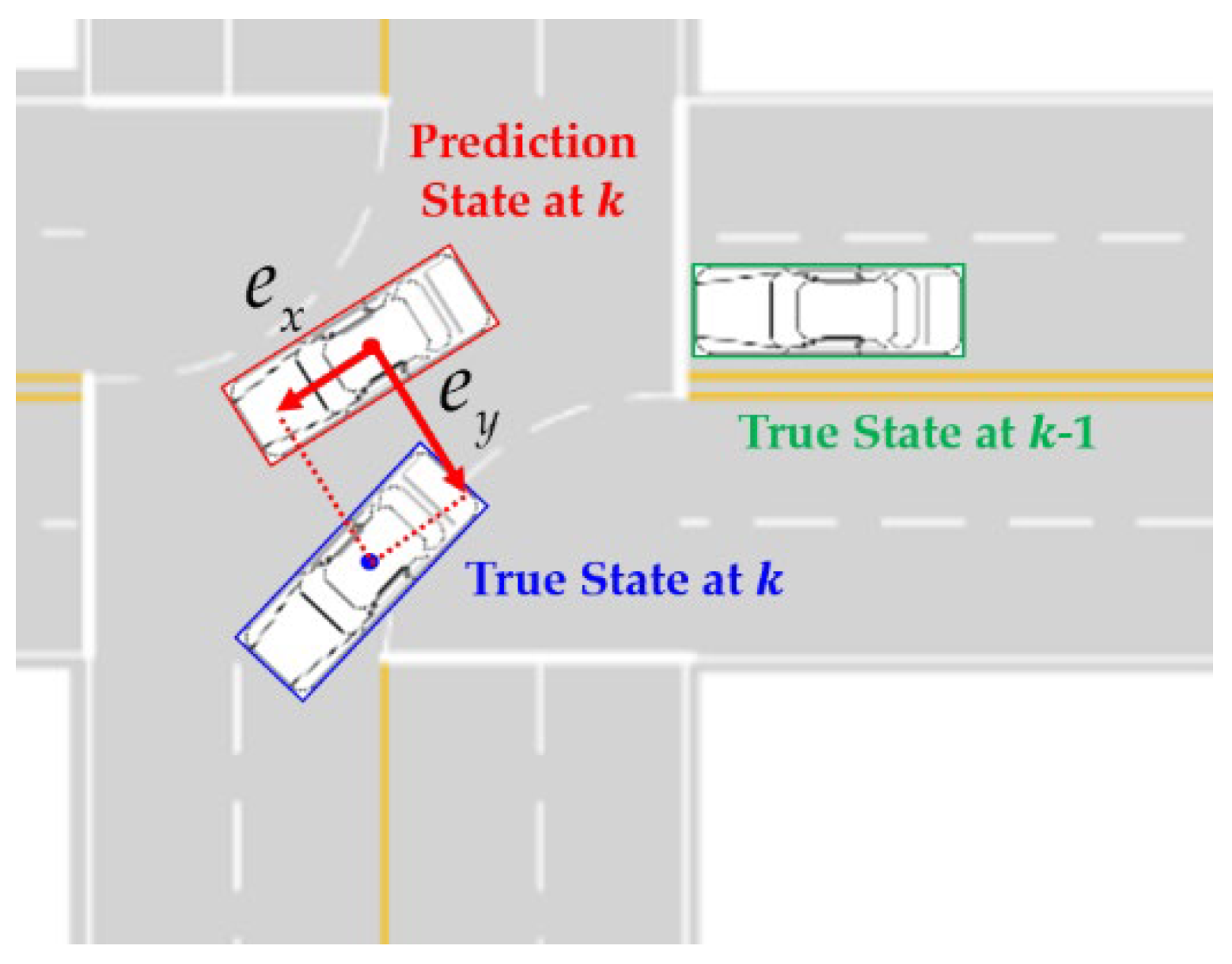
In the previous chapter, the target state prediction with the intention inference algorithm has been proposed based on the IMM approach. Because the future states are predicted based on the present and past information, the prediction uncertainty inevitably exists regardless of the prediction methods. In addition, the level of uncertainty is dependent on the prediction algorithm and the quality of the object data from the perception algorithm. Therefore, a proper algorithm for uncertainty estimation is required to increase the safety and control performance of the prediction-based motion planner. In this study, a recursive covariance estimator has been used to estimate the prediction uncertainty of the prediction results [28]. Because the prediction algorithm is based on the process update model of the EKF using IDM, the recursive covariance estimator is applicable to estimate the process noise of each state, such as the position and velocity. The basic concept of the prediction uncertainty estimation is a comparison between the current true states and predicted states derived from the true states of the previous step. The graphical representation of the relationships is described in Figure 8.
The recursive covariance estimator assumes that the measurement noise is stationary. As mentioned in the previous chapter, the position of the target vehicle is defined in a fixed global coordinate, not a local coordinate of the autonomous vehicle. In other words, dDTC, the position of the state vector, is defined with respect to the conflict point on the intersection map. Therefore, the proposed prediction algorithm satisfies the assumption of the recursive covariance estimator. Since EKF is already used, the process update and measurement can be written in the linearized equation as follows:
where wk−1 and vk are the covariances of the prediction model and perception module. Ak−1, Bk−1, and C are the system matrix, input matrix, and output matrix, respectively. In this study, Ak−1 is the same matrix Fk in the previous section. In Equation (11), xk−1 is the vehicle state at (k−1), and xk is the predicted state using the prediction model. This means that xk is the first-step prediction results from the true state xk−1 using the above-linearized equation.
yk can be represented in terms of xk−1 as follows:
xk−1 is represented in terms of yk−1 as follows:
yk can be represented as follows by substituting (13) into (12):
In Equation (14), the only unknown term is wk−1. Because yk and yk−1 are the measurement from the perception algorithm, vk and vk−1 are the same measurement noise under the assumption of stationary. Therefore, the recursive estimator for wk−1 can be defined by multiplying M to (14) and introducing the new notations ξk and Vk:
The covariance of wk−1 is estimated as a recursive form as follows:
Using (16), the covariance of the process noise wk is estimated.
4. Target State Prediction with Uncertainty Estimation
It is necessary to consider the uncertainty of the prediction in order to improve the safety and performance of autonomous vehicles on urban roads. Therefore, this study integrates the SMPC approach with the prediction uncertainty estimator to improve the performance of SMPC by updating the probability distribution of chance constraints every moment. Before discussing SMPC, the driving mode and constraints are properly defined based on the predicted states of intersection-approaching vehicles. Therefore, the robust motion planner for intersection passing is composed of three sub-modules: The driving mode decision, the defining prediction-based constraint, and solving SMPC. The details of each module will be discussed in the following sections.
4.1. Driving Mode Decision
Constraints for SMPC are highly related to the driving mode because intersection cross priority decides the boundaries of constraints. Therefore, the driving mode should be determined before defining the constraints for SMPC. In this study, driving modes are composed of three modes: ‘Approach’, ‘Cross’, and ‘Yield’. The approach mode is prepared to provide safe approaching behavior at the uncontrolled intersection until the target is detected. It means that the driver’s deceleration characteristics are reflected in autonomous driving as an approach mode to avoid the inevitable collision with targets appearing from a blind spot. The deceleration command of the approach mode is determined based on the shape of the occluded region, the possible target-appearing position, and the nominal braking characteristics of the human driver.
Meanwhile, the cross and yield modes are declared when the autonomous vehicles detect other intersection-approaching targets. In these driving modes, the risk caused by the target vehicle should be properly managed by the interaction between the autonomous vehicle and targets. Then, an SMPC-based motion planner is used to determine the desired acceleration. Particularly, yield mode is the replacement of the stop mode of the previous studies to cover most driving situations except when the ego vehicle has a cross priority. Therefore, an autonomous vehicle in yield mode does not simply stop but determines various behaviors according to the driving situation.
A mode transition condition between the cross and yield modes is defined based on the uncontrolled intersection theory. The uncontrolled intersection theory has been used to analyze the driving behavior of human drivers who are interacting with each other in uncontrolled intersections. The concepts of critical gap and follow-up gap have been used to define the mode transition condition between the cross and yield modes. In the uncontrolled intersection theory, the critical gap is the threshold for the time gap between higher-rank stream vehicles. It means that no driver will split the vehicle stream from a higher-rank road unless the gap between the vehicle in a higher priority stream is at least equal to the critical gap. The follow-up gap is the threshold to follow the preceding vehicle that enters the intersection. The driver will enter the intersection if the headway time with a preceding vehicle is less than the follow-up gap.
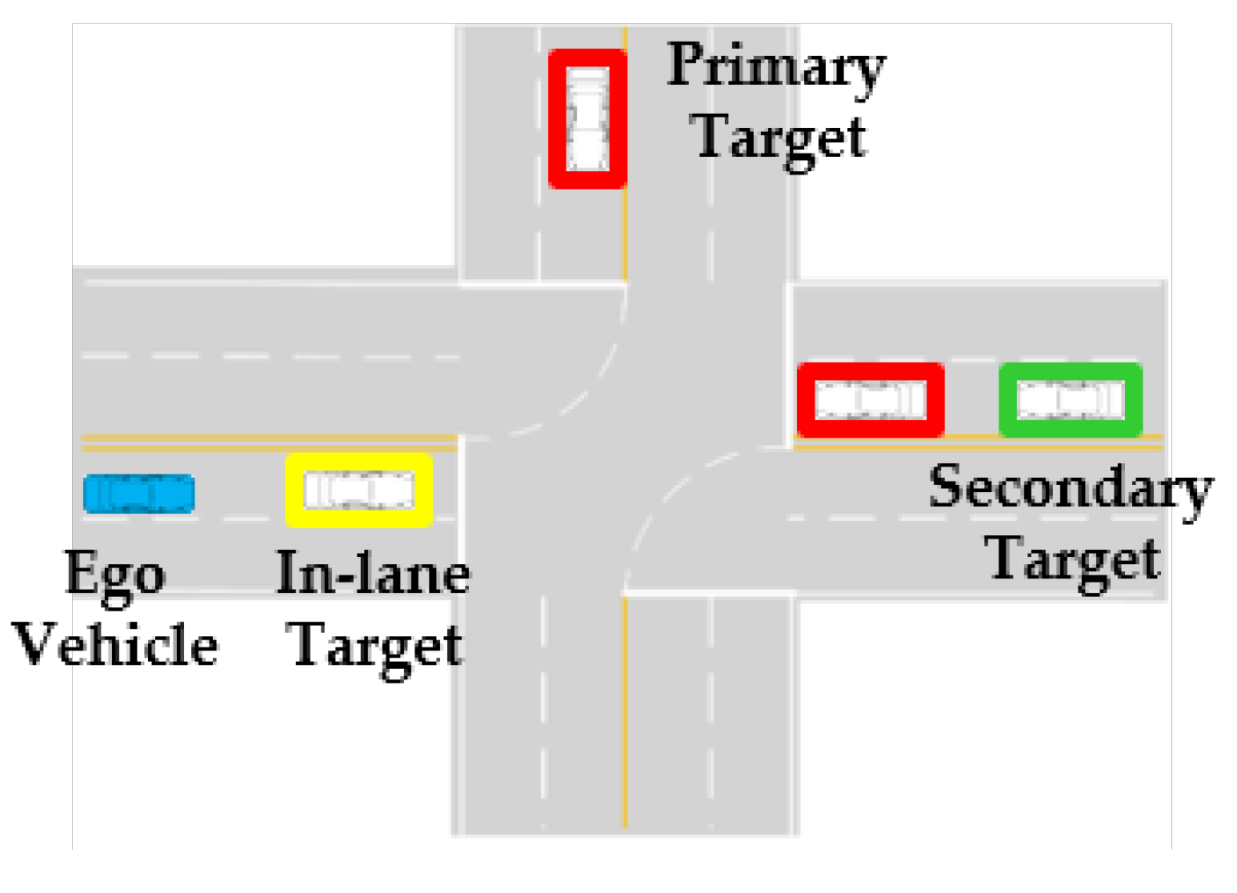
This concept has been modified to define the mode transition condition for the proposed driving-mode decision algorithm. First, the approaching targets have been classified into three groups, primary, secondary, and in-lane targets, as shown in Figure 9. The first vehicle entering the intersection from other branches of the ego vehicle is denoted as a primary target. Then, the next vehicle immediately following the primary target is classified as a secondary target. The in-lane target means the preceding target of the ego vehicle. Based on the target classification, a time gap between primary and secondary targets is compared to the critical gap. A headway time between the in-lane target and ego vehicle is compared to the follow-up gap. When calculating the time gap and headway time, the predicted states of the ego and the target vehicle have been used to overcome the limitations of the constant velocity assumption.
The driving mode is changed to yield mode if one of the following conditions is satisfied: (1) The remaining time to the intersection is larger than the primary target, (2) the time gap between primary and secondary target is smaller than the critical gap threshold, or (3) the headway time to the preceding vehicle is larger than the follow-up gap threshold. On the contrary, the cross mode is only declared if the opposites of the aforementioned conditions are all satisfied simultaneously. This hard condition for the cross mode is introduced to prevent a dangerous situation caused by misjudgment of the driving mode. In this study, a critical gap threshold of 4 s and a follow-up gap threshold of 2 s has been used [29,30,31]. In addition, the transition margin of a 1s base has been added to avoid chattering between driving modes.
4.2. Stochastic Model Predictive Controller
The first step of designing the SMPC-based motion planner is defining the plant model [32]. The state-space model of the longitudinal dynamics is defined by considering the characteristics of the longitudinal actuator. The delay of the acceleration and braking can be modeled as a first-order delay model. Therefore, the first-order input delay model has been employed to define a longitudinal model. The state and input vectors are defined as follows:
where p[k], v[k], and a[k] are the position, velocity, and acceleration of the ego vehicle on the curvilinear coordinate along the desired trajectory of the ego vehicle. ades,[k] is the longitudinal acceleration input, which is determined by solving the SMPC problem. Based on the state and input vectors, the longitudinal dynamics are defined as follows:
where dt and τx are the sampling time of the SMPC solver and the acceleration delay constant of the actuator.
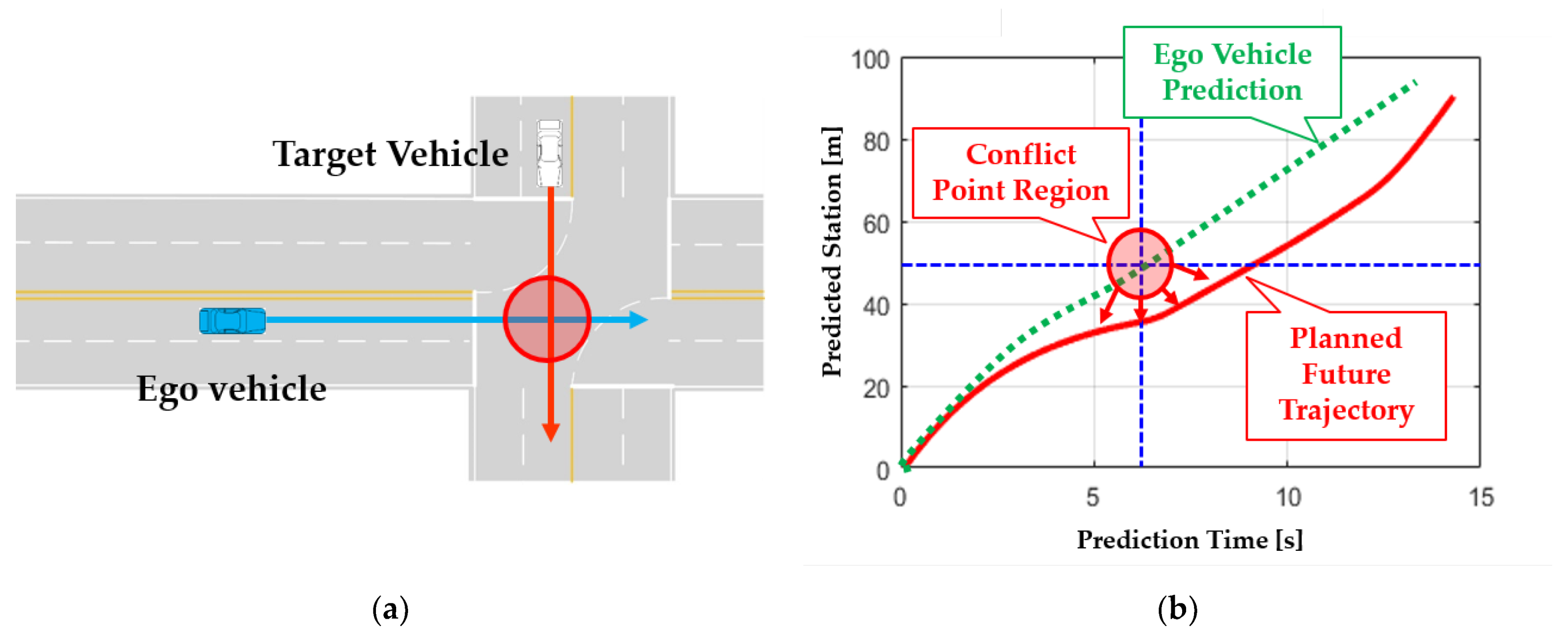
The next step is defining the constraints for the SMPC problem. The concept of intersection motion planning is described in Figure 10. The example scenario is the primary target-only case where a single conflict point region is predicted inside the intersection as shown in Figure 10a. This conflict point region can be defined based on the prediction time vs. the predicted station plane as shown in Figure 10b. When defining the conflict point region, the prediction results of the ego vehicle under the assumption of the cross mode and the predicted states of the approaching target using the proposed predictor have been used to find the most probable conflict position and time. The constraints have been determined to avoid the conflict point region while considering the prediction uncertainty.
Constrains for the SMPC problem are categorized as chance constraints and deterministic constraints. The constraints related to the predicted states of the targets are defined as chance constraints. Meanwhile, the dynamics, actuator limitation, and initial condition correspond to the deterministic constraints. As mentioned before, the predicted states of the target are used to define the conflict point region. Therefore, the position constraint should consider the uncertainty of target state prediction. In other words, the position constraint is designed as a chance constraint. The inequalities of the position constraint are defined as follows:
where TTCconf,min and Cconf,min are the minimum value of TTCconf and Cconf from the human driving data analysis. [k],1 and [k],2 are the predicted position and velocity of the target vehicle, which have uncertainty. Pego is the base constraint that follows the predicted states of the ego vehicle, which is represented as a green dotted line in Figure 10b. c[k] is the coupled term between the optimal state of the ego vehicle and the predicted state of the target vehicle. Therefore, (19) has a stochastic variable as a form of an inequality constraint. In other words, (19) is the chance constraint of the SMPC problem. Therefore, the position constraints are redefined as follows:
where β is the lower boundary for the probability of the inequality equations. The standard deviation of the probability distribution is defined as an estimation result of the recursive covariance matrix. It means that the inequality constraints are adaptively adjusted according to the perception performance and the accuracy of the behavior predictor.
The position constraint is defined differently for the corresponding driving mode. For the yield mode, the ego vehicle avoids the collision using braking, which means an upper limit is assigned. For the cross mode, the ego vehicle has a priority to pass the conflict point first then the target vehicle. In this case, a lower limit has been applied to the position constraint.
The constraints for v[k], a[k], and [k] are defined as a deterministic constraint as follows:
where vmax and vcurve are the velocity limit and velocity derived from the maximum lateral acceleration and road curvature. amin, amax, and max are the minimum acceleration, maximum acceleration, and maximum jerk for longitudinal motion, respectively. The parameters used for the SMPC problem are summarized in Table 1.
The initial conditions are defined as the current states of the ego vehicle.
Based on these constraints, the SMPC problem has been designed to calculate the desired longitudinal acceleration. The cost function for the SMPC problem is formulated as follows:
where xref,[k] is the ego vehicle prediction results, which are depicted as a green dotted line in Figure 10b. Q and R are the weighting matrices of the cost function. Np is the size of the prediction horizon of the SMPC problem. The cost function is designed to minimize the deviation from the ego vehicle prediction results and control effort. Therefore, the SMPC problem calculates the control inputs that minimize the change of behavior of the cross mode and the acceleration usage. The solver FORCES is utilized to solve the SMPC problem in the MATLAB/Simulink environment [33].
5. Results
The proposed motion planner based on SMPC with a recursive uncertainty estimator has been evaluated through computer simulation for a Left-Turn Across-Path–Opposite Direction (LTAP-OD) scenario and the arbitrary scenario with multi-traffic. For simulation under the arbitrary scenario, the Monte Carlo simulation approach has been used to randomly generate the initial condition and driving route of target vehicles. The simulation environment has been constructed based on MATLAB/Simulink R2021a and CarSim 8.02.
5.1. Case Study
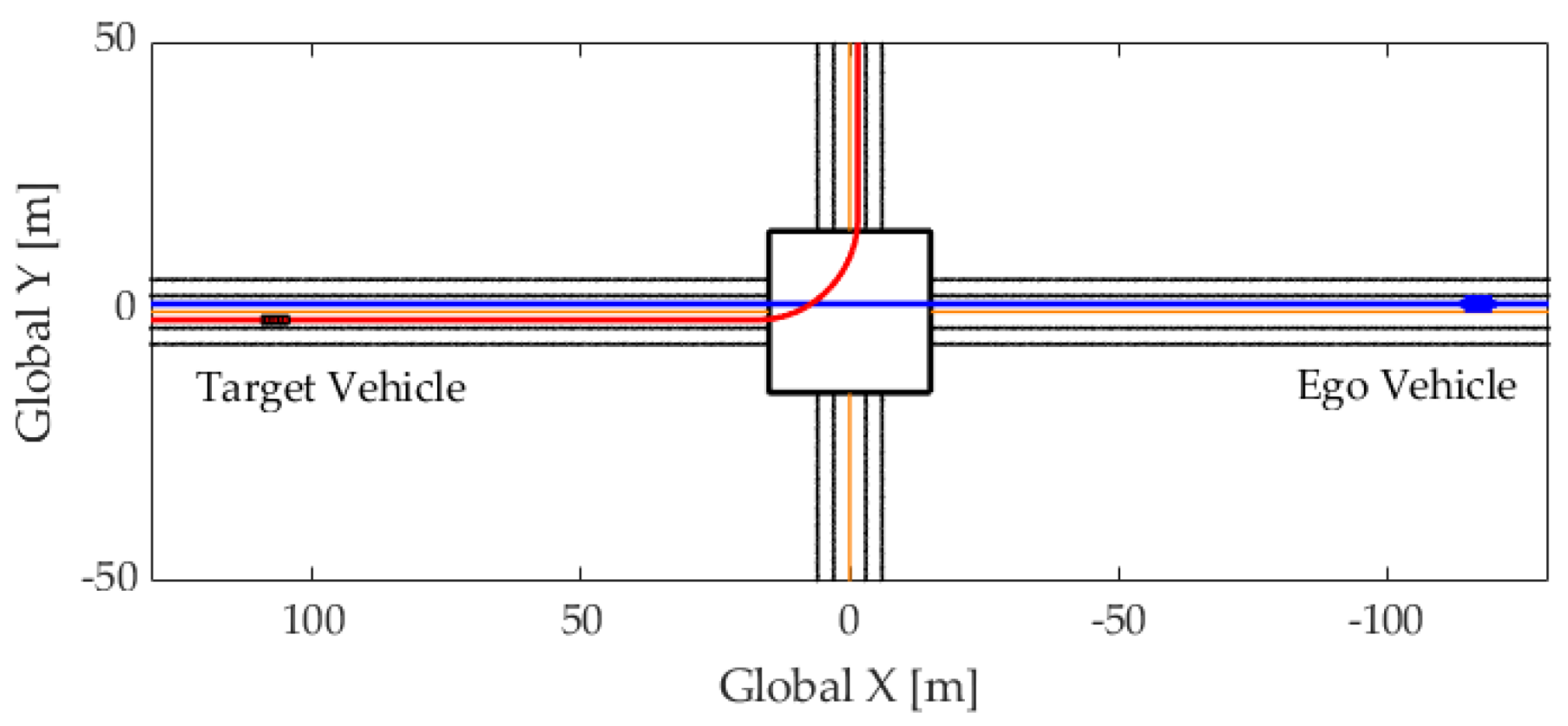
The simulation scenario for the case study is described in Figure 11. The LTAP-OD scenario has been used for the evaluation of the proposed and base algorithms. The SMPC without an uncertainty estimator is denoted as a base algorithm in this chapter. In the conventional LTAP-OD scenario, the subject vehicle tries to turn left while oncoming targets are going straight. In this study, LTAP-OD has been modified to swap the driving route of the ego and target vehicles. In other words, the target vehicle turns left while the ego vehicle attempts to pass straight through the intersection. The values of initial dDTI,ego of 80 m, initial dDTI,target of 60 m, the initial velocity of 45 km/h, and the maximum velocity of 50 km/h have been used as an initial condition. The difference in the initial condition of dDTI was intended to make the target vehicle enter the intersection first, which creates the situation where the ego vehicle will yield. Under the same initial condition, the simulation has been performed three times for each algorithm with different levels of sensor noise. In each of the three simulation runs, the measurement noise of the environment sensor and perception algorithm has been assumed to be a normal distribution. The standard deviation of the sensor noise has been set to 0.5-times, 1 time, and 2 times the reference value from the quantitative analysis of the previous study [25].
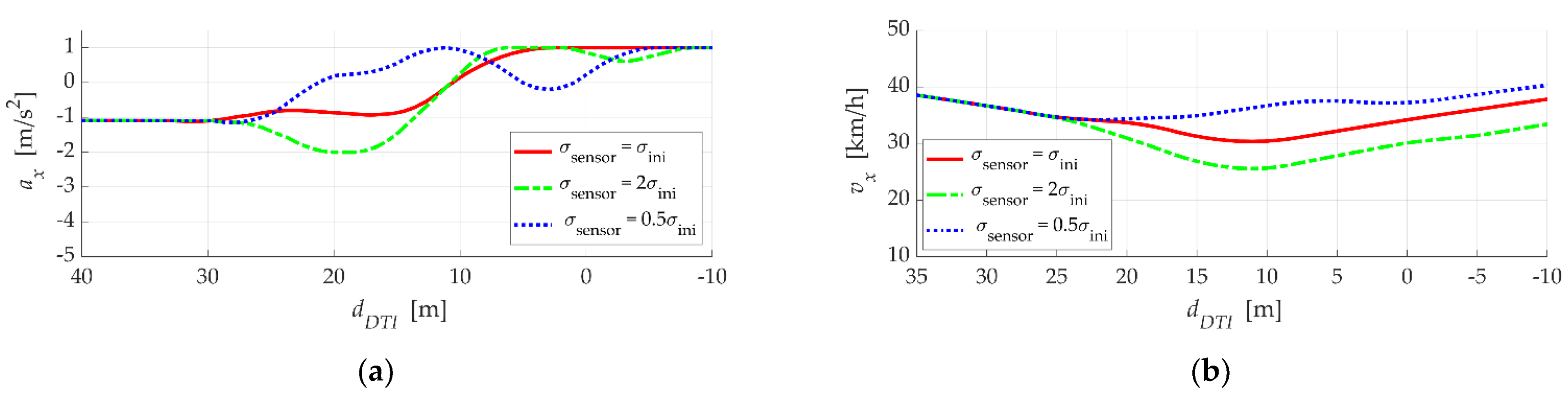
The simulation results of the proposed and base algorithms have been summarized in Figure 12 and Figure 13, respectively. A history of the variables has been represented with respect to the dDTI to prevent the misinterpretation caused by a different driving time. As shown in Figure 12 and Figure 13, the behavior changes of the ego vehicle occurred at dDTI = 30 m, where the target vehicle was detected by the sensor model for the first time. The driving mode of all simulations was transitioned to yield mode after target detection. As a result of the simulation, it can be confirmed that the TTCconf and Cconf were maintained above the TTCconf,min and Cconf,min in all simulation cases. However, the difference in behavior shown in the simulation results was significant.
From the simulation results of the proposed algorithm shown in Figure 12, it can be confirmed that the response to the perception and prediction uncertainty has been effectively made. The magnitude of the deceleration command is proportional to the sensor noise level because the probability distribution of the chance constraint is adapted to the uncertainty estimate from the recursive covariance estimator. Specifically, the amount of the deceleration is increased to respond to large uncertainty of the σsensor = 2 σini case. Then, in a situation where the influence of uncertainty is reduced due to the decrease in Cconf, the acceleration command is generated earlier than the σsensor = σini case because the safety margin is already secured. In the case of σsensor = 0.5 σini, the SMPC can trust the prediction results more than other cases, because the prediction algorithm estimates the small uncertainty. Therefore, the risk caused by approaching targets can be managed at a point close to the conflict point region. The braking command is generated at a later moment than the other two cases. As the proposed algorithm can actively respond to the uncertainty of the sensor, the trajectories of TTCconf vs. Cconf show a similar shape while complying with the constraints for TTCconf and Cconf.
The simulation result of the base algorithm shows the opposite tendency to the proposed algorithm, and it can be seen that more deceleration is utilized to manage the risk. Because the covariance of the chance constraint is set to σini, the simulation result of the σsensor = σini case is the same as the proposed algorithm. However, the sensor noise differed from the σini, and different behavior was observed as shown in Figure 13. In the case of σsensor = 2 σini, the predicted states of the target are overly trusted, which means the delayed braking is close to the conflict point region. On the other hand, the uncertainty is excessively considered in the σsensor = 0.5 σini case, which causes deceleration to occur earlier. In both simulation cases, the minimum safety specifications TTCconf,min and Cconf,min were satisfied, but the base algorithm was unable to respond to changes of perceived uncertainty and showed discomfort behavior for passengers and surrounding vehicles. In short, the simulation results for the LTAP-OD scenario have shown that the proposed algorithm can manage the uncertainty of perception and prediction when passing through the uncontrolled intersection.
5.2. Monte Carlo Simulation
Monte Carlo simulation has been conducted to evaluate the proposed algorithm in various situations. The test scenario has been generated by randomly selecting the sensor noise level, initial position, initial velocity, maximum velocity, and the driving route of the target vehicles. Five target vehicles have been used when configuring the test scenarios. Sets of the sensor noise, initial position, initial velocity, and maximum velocity are generated by using a normal distribution as follows:
The example case of the Monte Carlo simulation scenario is shown in Figure 14.
A total of 100 simulations were performed for both algorithms. The distributions of the simulation result on the TTCconf vs. Cconf plane are depicted in Figure 15. As the two vehicles approach the intersection, the TTCconf and Cconf decrease, and trajectories are headed to the origin of the TTCconf vs. Cconf plane. Then, the motion planner applied braking inputs to manage the risks caused by approaching targets and prevent the reduction of TTCconf. After the target vehicle passing through the intersection, TTCconf and Cconf increase to the right top of the TTCconf vs. Cconf plane. From this point of view, it can be seen that the proposed algorithm maintains its control performance robustly against changes in sensor uncertainty from the distribution toward the top right side of the TTCconf vs. Cconf plane. On the other hand, the results of the base algorithm show that few trajectories are heading to the top right. This shows that the base algorithm does not have the ability to respond to changes in sensor uncertainty. In particular, since the risk was not properly assessed, the braking input was increased only after TTCconf,min and Cconf,min were exceeded. In other words, the results of the proposed algorithm were maintained above the safety constraints TTCconf,min and Cconf,min. However, the base algorithm cannot guarantee the safety constraints, even though more deceleration was used.
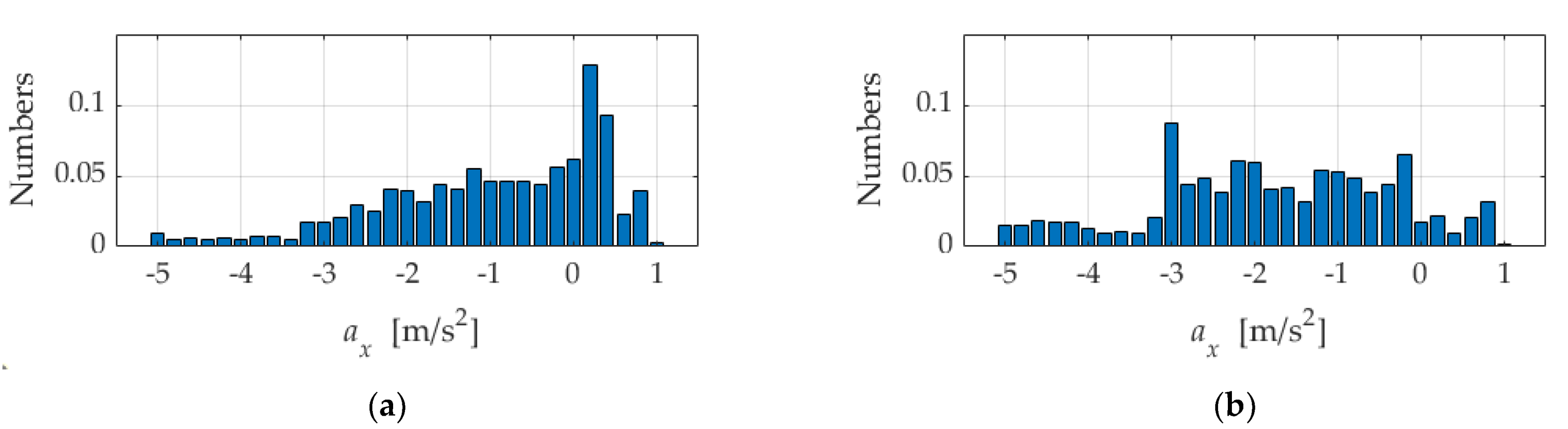
In order to analyze the ride comfort of both algorithms, the histogram of the acceleration usage is illustrated in Figure 16. The acceleration usage of the proposed algorithm was concentrated near 0 m/s2 and most of it is in the range of −3 to 1 m/s2, which is the typical range of human drivers. However, the histogram of the base algorithm is evenly distributed between −3 to 1 m/s2. In addition, hard braking below −3 m/s2 is often used. This difference can be explained based on the shape difference of the trajectory on the TTCconf vs. Cconf plane shown in Figure 15. As mentioned before, the base algorithm does not guarantee the minimum constraints, and in this situation, maximum deceleration is generated. As a result, hard braking below −3 m/s2 occurs frequently as shown in Figure 16b. Meanwhile, the proposed algorithm proactively applies braking before the risk increases, and risk is appropriately managed with minimal hard braking. Therefore, the proposed algorithm achieves both safety and ride comfort compared to the base algorithm.
From the perspective of computational time, the proposed SMPC-based motion planner was able to determine the desired acceleration within 30 ms even though the algorithm was implemented in MATLAB/Simulink environments. When implemented on an autonomous vehicle, a velocity controller calculates the throttle and brake inputs with much faster sampling to track the target acceleration determined by the proposed algorithm. In addition, since the speed of the vehicle is not fast in the uncontrolled intersection driving situation, the error caused by the calculation time of 30 ms is not significant. Furthermore, since the 30 ms is shorter than the typical LiDAR or camera sensor processing time, a sampling time of 30 ms is fast enough to determine the target motion based on environmental information. For example, the LiDAR-based environment perception system used to collect driving data in this study has a sampling time of 40 ms. Therefore, the proposed algorithm can be applied to an autonomous vehicle.
6. Conclusions
A stochastic model predictive control-based motion-planning algorithm for uncontrolled intersections has been developed and evaluated with computer simulation. The proposed SMPC problem has been improved by integrating it with a prediction uncertainty estimator. The future states of target vehicles have been predicted using an interacting multiple-model filter based on human behavior models. The intelligent driver model has been used to define the behavior model and process update of the IMM filter. The uncertainty of the sensor measurement and prediction has been estimated by using the recursive covariance estimator. The driving mode has been determined using the estimated time to arrive at the intersection, the critical gap, and the follow-up gap. The desired acceleration of autonomous vehicles has been determined using the SMPC approach considering the safety indexes, predicted states of ego and target vehicles, prediction uncertainty, and driving mode. Simulation studies have been conducted to evaluate the proposed algorithm. The results of the left-turn across-path–opposite direction scenario showed that the integrated approach of an uncertainty estimator and SMPC improve the robustness of perception performance. The results of the Monte Carlo simulation showed the proposed algorithm to guarantee the minimum safety level and improve the ride comfort compared to the base algorithm without uncertainty estimation.
The proposed integrated approach can be extended to situations where prediction uncertainty can affect the performance of the motion planning of autonomous driving. For example, decision and motion planning for lane changing, overtaking, and roundabout scenarios can improve the safety and performance of an autonomous vehicle driving with human drivers. In future studies, the proposed motion planner for intersections will be extended to the path-planning algorithm within the intersection as well as the prediction error estimation for lateral motion. In other words, the algorithm for an uncontrolled intersection will cover the prediction of the surrounding vehicles and motion planning in both directions, longitudinally and laterally. In addition, the model-based predictor will be improved by introducing learning-based approaches to effectively reflect the driving characteristics of the drive.
Funding
This study was supported by the Research Program funded by the SeoulTech (Seoul National University of Science and Technology).
Institutional Review Board Statement
Not applicable.
Informed Consent Statement
Not applicable.
Data Availability Statement
Not applicable.
Conflicts of Interest
The authors declare no conflict of interest.
References
- Maile, M.; Zaid, F.A.; Caminiti, L.; Lundberg, J.; Mudalige, P. Cooperative Intersection Collision Avoidance System Limited to Stop Sign and Traffic Signal Violations; RITA: Washington, DC, USA, 2008; DOT-HS-811-048. [Google Scholar]
- Bougler, B.; Cody, D.; Nowakowski, C. California Intersection Decision Support: A Driver-Centered Approach to Left-Turn Collision Avoidance System Design; PATH: Berkeley, CA, USA, 2008; UCB-ITS-PRR-2008-1. [Google Scholar]
- Poch, M.; Mannering, F. Negative binomial analysis of intersection-accident frequencies. J. Transp. Eng. 1996, 122, 105–113. [Google Scholar] [CrossRef] [Green Version]
- Polus, A. Driver behaviour and accident records at unsignalized urban intersections. Accid. Anal. Prev. 1985, 17, 25–32. [Google Scholar] [CrossRef]
- Hubmann, C.; Becker, M.; Althoff, D.; Lenz, D.; Stiller, C. Decision making for autonomous driving considering interaction and uncertain prediction of surrounding vehicles. In Proceedings of 2017 IEEE Intelligent Vehicles Symposium, Los Angeles, CA, USA, 11–14 June 2017; pp. 1671–1678.
- Hubmann, C.; Schulz, J.; Becker, M.; Althoff, D.; Stiller, C. Automated driving in uncertain environments: Planning with interaction and uncertain maneuver prediction. IEEE Trans. Intell. Veh. 2018, 3, 5–17. [Google Scholar] [CrossRef]
- Qiao, Z.; Muelling, K.; Dolan, J.; Palanisamy, P.; Mudalige, P. POMDP and hierarchical options MDP with continuous actions for autonomous driving at intersections. In Proceedings of the 2018 21st International Conference on Intelligent Transportation Systems, Maui, HI, USA, 4–7 November 2018; pp. 2377–2382. [Google Scholar]
- Brechtel, S.; Gindele, T.; Dillmann, R. Probabilistic decision-making under uncertainty for autonomous driving using continuous POMDPs. Proceedings of 17th international IEEE conference on intelligent transportation systems, Qingdao, China, 8–11 October 2014; pp. 392–399. [Google Scholar]
- Noh, S. Decision-making framework for autonomous driving at road intersections: Safeguarding against collision, overly conservative behavior, and violation vehicles. IEEE Trans. Ind. Electron. 2019, 66, 3275–3286. [Google Scholar] [CrossRef]
- Lu, G.; Li, L.; Wang, Y.; Zhang, R.; Bao, Z.; Chen, H. A rule based control algorithm of connected vehicles in uncontrolled intersection. In Proceedings of the 17th international IEEE conference on intelligent transportation systems, Qingdao, China, 8–11 October 2014; pp. 115–120. [Google Scholar]
- Li, G.; Li, S.; Li, S.; Qin, Y.; Cao, D.; Qu, X.; Cheng, B. Deep reinforcement learning enabled decision-making for autonomous driving at intersections. Automot. Innov. 2020, 3, 374–385. [Google Scholar] [CrossRef]
- Xihui, W. Predictive Motion Planning of Vehicles at Intersection Using a New GPR and RRT. In Proceedings of the 2020 IEEE 23rd International Conference on Intelligent Transportation Systems, Rhodes, Greece, 20–23 September 2020; pp. 1–6. [Google Scholar]
- Schildbach, G.; Soppert, M.; Borrelli, F. A collision avoidance system at intersections using robust model predictive control. In Proceedings of the 2016 IEEE Intelligent Vehicles Symposium, Gothenburg, Sweden, 19–22 June 2016; pp. 233–238. [Google Scholar]
- Nilsson, J.; Brännström, M.; Fredriksson, J.; Coelingh, E. Longitudinal and lateral control for automated yielding maneuvers. IEEE Trans. Intell. Transp. Syst. 2016, 17, 1404–1414. [Google Scholar] [CrossRef]
- Jeong, Y.; Yi, K. Target vehicle motion prediction-based motion planning framework for autonomous driving in uncontrolled intersections. IEEE Trans. Intell. Transp. Syst. 2021, 22, 168–177. [Google Scholar] [CrossRef]
- Nor, M.H.M.; Namerikawa, T. Optimal Motion Planning of Connected and Automated Vehicles at Signal-Free Intersections with State and Control Constraints. SICE J. Control, Meas. Syst. Integr. 2020, 13, 30–39. [Google Scholar]
- Medina, A.I.M.; van de Wouw, N.; Nijmeijer, H. Cooperative intersection control based on virtual platooning. IEEE Trans. Intell. Transp. Syst. 2017, 19, 1727–1740. [Google Scholar] [CrossRef] [Green Version]
- Choi, M.; Rubenecia, A.; Choi, H.H. Reservation-based traffic management for autonomous intersection crossing. Int. J. Distrib. Sensor Netw. 2019, 15, 1–15. [Google Scholar] [CrossRef] [Green Version]
- Qian, B.; Zhou, H.; Lyu, F.; Li, J.; Ma, T.; Hou, F. Toward collision-free and efficient coordination for automated vehicles at unsignalized intersection. IEEE Internet Things J. 2019, 6, 10408–10420. [Google Scholar] [CrossRef]
- Tian, R.; Li, N.; Kolmanovsky, I.; Yildiz, Y.; Girard, A.R. Game-theoretic modeling of traffic in unsignalized intersection network for autonomous vehicle control verification and validation. IEEE Trans. Intell. Transp. Syst. in press. [CrossRef]
- Jeong, Y.; Yi, K.; Park, S. SVM based intention inference and motion planning at uncontrolled intersection. IFAC-PapersOnLine 2019, 52, 356–361. [Google Scholar] [CrossRef]
- Jeong, Y.; Kim, S.; Yi, K. Surround vehicle motion prediction using LSTM-RNN for motion planning of autonomous vehicles at multi-lane turn intersections. IEEE Open J. Intell. Transp. Syst. 2020, 1, 2–14. [Google Scholar] [CrossRef]
- Hafner, M.R.; Cunningham, D.; Caminiti, L.; Del Vecchio, D. Automated vehicle-to-vehicle collision avoidance at intersections. In Proceedings of the World Congress on Intelligent Transport Systems, Orlando, FL, USA, 16–20 October 2011; pp. 1–11. [Google Scholar]
- Chen, Y.; Zha, J.; Wang, J. An autonomous T-intersection driving strategy considering oncoming vehicles based on connected vehicle technology. IEEE/ASME Trans. Mechatron. 2019, 24, 2779–2790. [Google Scholar] [CrossRef]
- Lee, H.; Yoon, J.; Jeong, Y.; Yi, K. Moving Object Detection and Tracking Based on Interaction of Static Obstacle Map and Geometric Model-Free Approach for Urban Autonomous Driving. IEEE Trans. Intell. Transp. Syst. in press. [CrossRef]
- Liebcner, M.; Klanner, F.; Baumann, M.; Ruhhammer, C.; Stiller, C. Velocity-based driver intent inference at urban intersections in the presence of preceding vehicles. IEEE Intell. Transp. Syst. Mag. 2013, 5, 10–21. [Google Scholar] [CrossRef] [Green Version]
- Mazor, E.; Averbuch, A.; Bar-Shalom, Y.; Dayan, J. Interacting multiple model methods in target tracking: A survey. IEEE Trans. Aerosp. Electron. Syst. 1998, 34, 103–123. [Google Scholar] [CrossRef]
- Feng, B.; Fu, M.; Ma, H.; Xia, Y.; Wang, B. Kalman filter with recursive covariance estimation—Sequentially estimating process noise covariance. IEEE Trans. Ind. Electron. 2014, 61, 6253–6263. [Google Scholar] [CrossRef]
- Troutbeck, R.J.; Brilon, W. Unsignalized Intersection Theory; Transportation Research Board: Washington, DC, USA, 1997; Special Rep. 165. [Google Scholar]
- Chan, C.Y. Characterization of driving behaviors based on field observation of intersection left-turn across-path scenarios. IEEE Trans. Intell. Transp. Syst. 2006, 7, 322–331. [Google Scholar] [CrossRef]
- Weinert, A. Estimation of critical gaps and follow-up times at rural unsignalized intersections in Germany. In Proceedings of the Fourth International Symposium on Highway Capacity, Maui, HI, USA, 27 June–1 July 2000; pp. 409–421. [Google Scholar]
- Mesbah, A. Stochastic model predictive control: An overview and perspectives for future research. IEEE Control Syst. Mag. 2016, 36, 30–44. [Google Scholar]
- Chae, H.; Jeong, Y.; Lee, H.; Park, J.; Yi, K. Design and implementation of human driving data–based active lane change control for autonomous vehicles. Proc. Inst. Mech. Eng. D 2021, 235, 55–77. [Google Scholar] [CrossRef]
Figure 1.
Overall architecture of the autonomous driving system.

Figure 2.
Architecture of the proposed motion-planning algorithm for an uncontrolled intersection.

Figure 3.
Safety indexes for intersection driving scenario.

Figure 4.
Block diagram of IMM-based target intention inference algorithm.

Figure 5.
The measured and desired velocity profiles.

Figure 6.
Velocity profile of behavior models for target vehicle intention inference.

Figure 7.
Target state prediction results.

Figure 8.
Basic concepts of recursive covariance estimator-based prediction uncertainty estimation.

Figure 9.
Classification of intersection-approaching targets.

Figure 10.
Concept of the proposed motion planner. (a) Example scenario; (b) motion planning in predicted station vs. prediction time plane.
Figure 10.
Concept of the proposed motion planner. (a) Example scenario; (b) motion planning in predicted station vs. prediction time plane.

Figure 11.
LTAP-OD scenario for case study.

Figure 12.
Simulation results of the proposed algorithm. (a) History of longitudinal acceleration; (b) history of longitudinal velocity; (c) history of TTCconf; (d) trajectory of TTCconf and Cconf.
Figure 12.
Simulation results of the proposed algorithm. (a) History of longitudinal acceleration; (b) history of longitudinal velocity; (c) history of TTCconf; (d) trajectory of TTCconf and Cconf.


Figure 13.
Simulation results of the base algorithm. (a) History of longitudinal acceleration; (b) history of longitudinal velocity; (c) history of TTCconf; (d) trajectory of TTCconf and Cconf.
Figure 13.
Simulation results of the base algorithm. (a) History of longitudinal acceleration; (b) history of longitudinal velocity; (c) history of TTCconf; (d) trajectory of TTCconf and Cconf.

Figure 14.
Example simulation scenario of Monte Carlo simulation.

Figure 15.
Simulation results of the Monte Carlo simulation: (a) Proposed algorithm in vx; (b) proposed algorithm in ax; (c) base algorithm in vx; (d) base algorithm in ax.
Figure 15.
Simulation results of the Monte Carlo simulation: (a) Proposed algorithm in vx; (b) proposed algorithm in ax; (c) base algorithm in vx; (d) base algorithm in ax.

Figure 16.
Acceleration usage comparison: (a) Proposed algorithm; (b) base algorithm.


Table 1.
Parameters for SMPC problem.
| Symbol | Values | Symbol | Values |
|---|---|---|---|
| dt | 0.2 s | vmax | 50 km/h |
| τx | 0.5 s | amax | 1 m/s2 |
| Np | 25 | amin | −5 m/s2 |
| TTCconf,min | 2.0 s | max | 2 m/s3 |
| Cconf,min | 5.0 m | β | 0.95 |
Publisher’s Note: MDPI stays neutral with regard to jurisdictional claims in published maps and institutional affiliations. |
© 2021 by the author. Licensee MDPI, Basel, Switzerland. This article is an open access article distributed under the terms and conditions of the Creative Commons Attribution (CC BY) license (https://creativecommons.org/licenses/by/4.0/).
Share and Cite
MDPI and ACS Style
Jeong, Y. Stochastic Model-Predictive Control with Uncertainty Estimation for Autonomous Driving at Uncontrolled Intersections. Appl. Sci. 2021, 11, 9397. https://doi.org/10.3390/app11209397
AMA Style
Jeong Y. Stochastic Model-Predictive Control with Uncertainty Estimation for Autonomous Driving at Uncontrolled Intersections. Applied Sciences. 2021; 11(20):9397. https://doi.org/10.3390/app11209397
Chicago/Turabian StyleJeong, Yonghwan. 2021. "Stochastic Model-Predictive Control with Uncertainty Estimation for Autonomous Driving at Uncontrolled Intersections" Applied Sciences 11, no. 20: 9397. https://doi.org/10.3390/app11209397
Note that from the first issue of 2016, this journal uses article numbers instead of page numbers. See further details here.