
Anticipating Future Behavior of an Industrial Press Using LSTM Networks
by
 , , and
Balduíno César Mateus
1,2,* ,
,
Mateus Mendes
3,4,* ,
,
José Torres Farinha
3,5 and
and
António Marques Cardoso
2
1
EIGeS—Research Centre in Industrial Engineering, Management and Sustainability, Lusófona University, Campo Grande, 376, 1749-024 Lisboa, Portugal
2
CISE—Electromechatronic Systems Research Centre, University of Beira Interior, Calçada Fonte do Lameiro, P–62001-001 Covilhã, Portugal
3
Polytechnic of Coimbra, ISEC, 3045-093 Coimbra, Portugal
4
Institute of Systems and Robotics, University of Coimbra, 3004-531 Coimbra, Portugal
5
Centre for Mechanical Engineering, Materials and Processes—CEMMPRE, 3030-788 Coimbra, Portugal
*
Authors to whom correspondence should be addressed.
Appl. Sci. 2021, 11(13), 6101; https://doi.org/10.3390/app11136101
Submission received: 30 April 2021
/
Revised: 24 June 2021
/
Accepted: 25 June 2021
/
Published: 30 June 2021
(This article belongs to the Special Issue Smart Services: Artificial Intelligence in Service Systems)
Abstract
:Predictive maintenance is very important in industrial plants to support decisions aiming to maximize maintenance investments and equipment’s availability. This paper presents predictive models based on long short-term memory neural networks, applied to a dataset of sensor readings. The aim is to forecast future equipment statuses based on data from an industrial paper press. The datasets contain data from a three-year period. Data are pre-processed and the neural networks are optimized to minimize prediction errors. The results show that it is possible to predict future behavior up to one month in advance with reasonable confidence. Based on these results, it is possible to anticipate and optimize maintenance decisions, as well as continue research to improve the reliability of the model.
1. Introduction
Modern processors, computers and high speed networks make it possible to acquire, transfer and store large quantities of data in real time. Acquisition and combination of data from different sensors makes it possible to gain an insightful view of the state of factories, industrial plants and other facilities. Large datasets can be constructed, stored and processed using information technologies such as Big Data, cloud computing, cutting-edge computing, and artificial intelligence tools. The Internet of Things (IoT) is a recent concept, which provides many benefits to different areas, such as maintenance and production management, because it facilitates the automation of tasks such as monitoring and maintenance. This results in the popularization of intelligent systems, which are highly dependent on Big Data [1] and are an important area of study, since they offer the tools and methods to acquire and process large volumes of data such as historical production processes, including many production and operating parameters.
Modern time-series and other data analysis techniques have been used with success for different tasks, such as freeway traffic analysis [2] and additive manufacturing [3]. Different approaches have also been proposed in the field of predictive maintenance [4,5]. Satisfactory results were obtained using Big Data records as support for PCA models, which resulted in a warning alarm several days before a potential failure happened [6].
Life cycle optimization has been an important concern for decades. A physical asset with proper maintenance will have a longer useful life with a greater return on investment for the organization [7].
Predictive maintenance requires good quality data. The information that is extracted from the online or offline data must be reliable, and so the results must be good enough to justify the investment in data collection and analysis. The process starts from the correct calibration of the reading sensors and equipment [8]. The data are then stored and processed using different models, such as Principal Component Analysis (PCA) and Neural Networks [9]. Maintenance planning involves the use of several algorithms, the most common being time series [10].
Maintenance of equipment in the industry becomes a sensitive and important point that affects the equipment’s operating time and efficiency [5]. This makes maintenance one of the strategic points for the development and growth of competitiveness vis-à-vis competitors. Chen and Tseng studied the total expected cost of maintaining a flotation system, including the cost of lost production, the cost of repairs, and the cost of standby machines [11].
Daniyan et al. propose the integration of Artificial Intelligence (AI) systems, which will bring many benefits in diagnosing condition problems of industrial machines [12]. They highlight the viability of AI that combines the use of Artificial Neural Networks (ANNs) with a dynamic time series model, for fault diagnostics, to optimize the equipment intervention time.
Hsu et al. demonstrated that neural networks can be a great technology in the support and decision making of large and small companies [13]. There is a trend to use those tools in predictive maintenance systems with the aim of making the prediction systems more intelligent [14].
According to Jimenez et al., there is a great effort in the development of predictive models for application in predictive maintenance [15]. Ayvaz and Alpay apply Long Short-Term Memory (LSTM) neural network approaches to predict real production data, obtaining satisfactory results, superior to conventional models [16]. In their study to improve maintenance planning to minimize unexpected stops, they apply a new method that consists of the combined use of decomposition in empirical mode of ensemble and long-term memory. Their results showed a performance superior to other state of the art models.
LSTM networks use several ports with different functions to control neurons and to store information. The LSTM cell can retain important information for a longer period in which it is used. This property of information maintenance allows the LSTM to exhibit a good performance in the classification, processing, or forecasting of a complex dynamic sequences [17].
The present work uses different LSTM models to predict future trends of six variables, on a dataset containing three years of data samples grabbed in an industrial press, which aims to operate continuously with minimum downtime. Different data pre-processing techniques, network architectures and hyperparameters were tested in order to determine the models that best fit the data and provide the lowest prediction errors.
2. Related Work
2.1. Predictive Maintenance
In smart industries, predictive maintenance is one of the most used techniques to improve condition monitoring, as it allows one to evaluate the conditions of specific equipment in order to predict problems before failure [18]. For good performance of predictive models, it is important that the sensor data collected are of good quality. Deep neural models have been used with success to improve prediction for condition monitoring of industrial equipment.
Wang et al. [19] use a model of long short-term recurrent neural networks (LSTM-RNN) with the objective of predictive maintenance based on past data. The main objective of predictive maintenance is to make an accurate estimate of a system’s Remaining Useful Life (RUL). Traditional systems are only able to warn the user when it is too late and the failure occurs, causing an unpredictable offline period during which the system cannot operate properly with a consequent waste of time and resources [20].
In order to assess the condition of a system, the predictive maintenance approach employs sensors of different kinds. Some examples are temperature, vibration, velocity or noise sensors, which are attached to the main components whose failure would compromise the entire operation of the system. In this sense, predictive maintenance analyzes the history of a system in terms of the measurements collected by the sensors that are distributed among the components, with the objective of extracting a “failure pattern” that can be exploited to plan an optimal maintenance strategy and thus reducing offline periods [21]. In a case related to the steel industry, Ref. [22] used neural networks for classification of maintenance activities, so that interventions are planned according to the actual status of the machine and not in advance. Using multiple neural networks to identify status and RUL at a higher resolution can be very difficult, as the system can predict failure classifications and may not be able to recognize neighboring states. One limitation arises from the need for maintenance records to label datasets and the need for large amounts of data of adequate quality with maintenance events, such as component failures.
When systems start to be very complex or the number of sensor measurements to manage is very large, it can be difficult to estimate a failure. For this reason, in recent years, machine learning techniques are used more and more to predict working conditions of a component. Mathew et al. [23] propose several approaches to machine learning such as support vector machines (SVMs), decision trees (DTs), Random Forests (RFs), and others that show which technique has the best performance in RUL forecast for turbofan engines.
A major challenge in operations management is related to predicting machine speed, which can be used to dynamically adjust production processes based on different system conditions, optimize production performance and minimize energy consumption [24]. Essien and Giannetti [25] use a deep convolutional LSTM encoder–decoder architecture model on real data, obtained from a metal packaging factory. They show that it is possible to perform combinations of LSTM with other networks to significantly improve the results.
2.2. Prediction with LSTM Models
LSTM neural networks achieved the best performance in a number of computational sequence labeling tasks, including speech recognition and machine translation [26]. There are a variety of engineering problems that can be solved using predictive neural models. Beshrand Zarzoura used neural network models to predict problems of suspended road bridge structures based on global navigation satellite system observations [27]. Sak et al. demonstrated that the proposed LSTM architectures exhibit better performances compared to deep neural networks (DNNs) in a large vocabulary speech recognition task with a large number of output states [28]. Chen et al. adopted LSTMs for predicting the failure of heavy truck air compressors [29]. They concluded that the use of LSTMs leads to more consistency in predictions over time compared to models that ignore history, such as random forest models.
Gosh et al. [30] presented an extension that they called Contextual LSTM (CLSTM). This model was also used for the forecasting of pollutants. There is also the proposal for a genetic long short-term memory (GLSTM), which has been used in the study of wind energy forecasting [31]. Guo et al. presented a combination method based on real-time prediction errors in which the support vector regression (SVR) and LSTM outputs are combined in the final results of the model’s prediction, thus obtaining results of greater precision [32].
Ren et al. used a combination of a Convolution Neural Networks (CNNs) and LSTM in order to extract more in-depth information from data to predict the useful life of ion batteries [33]. Niu et al. used an LSTM and developed an effective speed prediction model to solve prediction problems over time [34]. Feng et al. report that the LSTM algorithm is superior and, according to them, it performs better than conventional neural network models [35].
The architecture of an LSTM network includes the number of hidden layers and the number of delay units, which is the number of previous data points that are considered for training and testing. Currently, there is no general rule for selecting the number of delays and hidden layers [36]. A deep LSTM can be built by stacking multiple LSTM layers, which generally works better than a single layer. Deep LSTM networks have been applied to solve many real-world sequence modelling problems [37]. The LSTM can also be used for planning studies [38], namely for planning the analysis of road traffic speed.
To produce a prediction model with good accuracy, it is necessary to optimize neural models’ hyperparameters. While simple models can often produce good results with default hyperparemeters, the optimization process can greatly improve the results [39,40,41]. The selection of hyperparameters often makes the difference between underperformance and state-of-the-art performance. Optimization is often performed using machine learning algorithms, such as grid search, grey wolf optimization or particle swarm optimization. In the present prediction model, however, the hyperparameters were optimized manually, following a trial and error guided process, one variable at a time. This method was followed because it was the most convenient considering the limited computing power available.
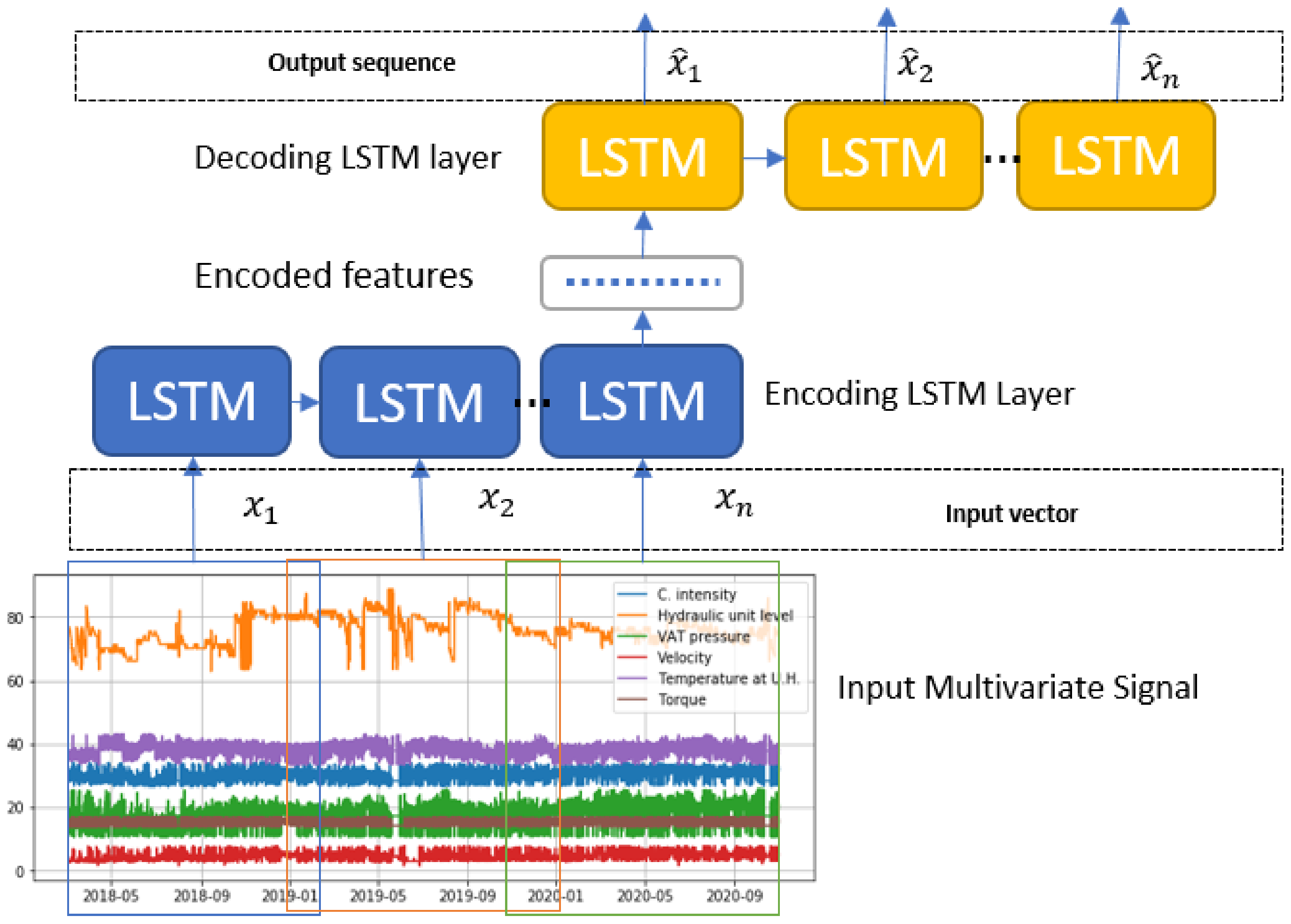
2.3. LSTM with Encoder and Decoder
Experiments were performed with a predictive model based on the LSTM with encoder and decoder architecture. The model consists of two LSTMs, in which the first LSTM has the function of processing an input sequence and generating an encoded state. The encoded state compresses the information in the input stream. The second LSTM, called a decoder, uses the encoded state to produce an output sequence. Those input and output sequences can be of different lengths.
This technique has already been used to solve problems such as the prediction of vehicle trajectories based on deep learning [42]. This architecture [43] has shown great performance for tasks of translating from sequence to sequence. LSTM encoder–decoder models have also been proposed for learning tasks such as automatic translation [43,44]. There is the application of this model to solve many practical problems, such as the study of the equipment condition, applications in language translations, among others [45,46,47].
3. Theoretical Background
The present work uses LSTM networks, considering the referred different studies showing their usefulness for time series predictions [48,49]. The LSTM is a deep learning recurrent neural network architecture that is a variation of traditional recurrent neural networks (RNNs). It was introduced by Hochreiter and Schmidhuber in 1997. The most popular version is a modification refined by many works in the literature [50,51], which is called vanilla LSTM (hereinafter referred to as LSTM). The LSTM is excellent at handling time series data only with its network parameters. For example, weights and polarization are adjusted or optimized [52]. The primary modification of the LSTM when compared to the RNN architecture is the structure of the hidden layer [53]. The LSTM model is a powerful type of recurrent neural network (RNN), capable of learning long-term dependencies [54]. They became popular due to their power of representation and effectiveness in capturing long-term dependencies [55].
Many networks showed instability when dealing with exploding or vanishing gradient problems during learning. Those problems happen when the gradient of the error is too large or too small. If it is too large, it overflows and the errors cannot propagate properly through different layers during learning. If it is too small, it vanishes and the network does not learn. Different methods were proposed to solve those problems, known as a kind of of “door control” that is used in RNN models. For example, Gated Recurrent unit (GRU) algorithms [56,57], as the LSTMs [58,59], are to a large extent immune to the gradient problems and learn well.
The LSTM network structure is based on three ports whose function is to regulate the flow. Those ports are called the entrance door, the forget gate, and the exit door. The main port of entry is to regulate the entry of new memory data; the forget gate has the function of regulating the storage time in the network memory and the output port intends to regulate how much the value retained in memory influences the activation of the output block [60].
Kong et al. demonstrate some relevant conclusions such as (1) LSTM has a good predictive capacity; (2) their use can significantly improve the profit of service providers, so there is an opportunity when it comes to exploring the forecast in real time [61]. LSTM networks are the de facto gold standard for deep learning algorithms for analyzing time series data [55].
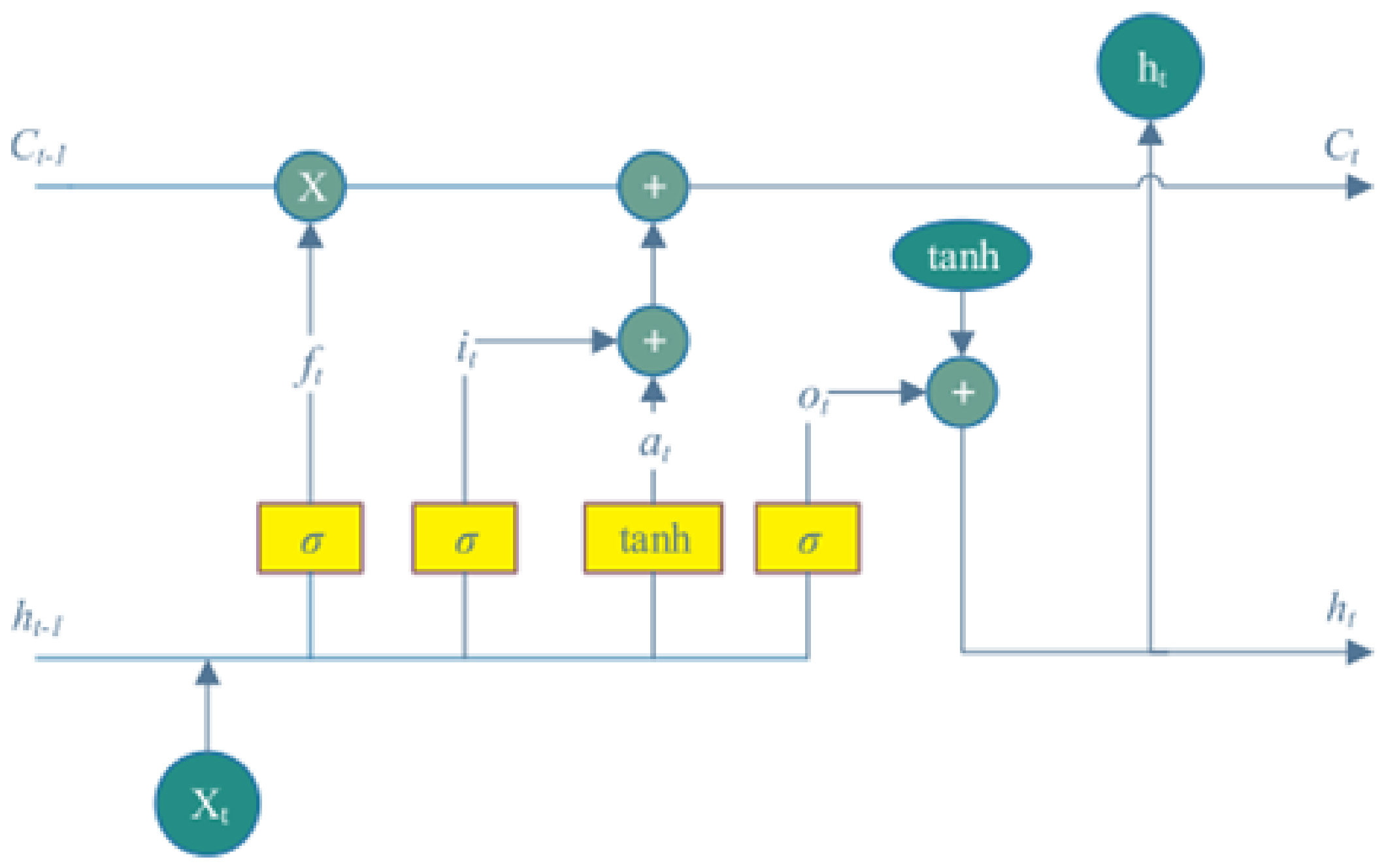
Figure 1 shows the internal architecture of an LSTM unit cell. According to [62,63], the internal calculation formulae of the LSTM unit are defined as follows:
where and are the weight matrices for mapping the current input layer on three ports and the state of the current input cell.
and are the weight matrices for mapping the previous output layer on three ports and the current state of the input cell. , and are polarization vectors for calculating the state of the door and the input cell. is the gate activation function, which is normally a sigmoid function. is the hyperbolic tangent function which is the activation function for the current state of the input cell.
Then, the current state of the output cell and the output layer can be calculated using the following equations.
To assess the quality of the prediction model, one of the most popular metrics is the Root Mean Square Error (RMSE), which is given by Equation (7):
where represents the desired (real) value and is the predicted (obtained from the model) value. The difference between Y and is the error between the value expected to obtain and the value actually obtained from the network. n represents the number of samples used in the test set.
The RMSE, however, is an absolute error. Therefore, there are also the Mean Absolute Percentage Error (MAPE) and the Mean Absolute Error (MAE). Those errors are given by the following formulae:
where represents the real value, the predicted value and n represents the total number of samples.
4. Data Preparation
Data are key to developing efficient modeling and planning. However, to be valuable, data need to be processed and structured before being analyzed.
4.1. The Problem
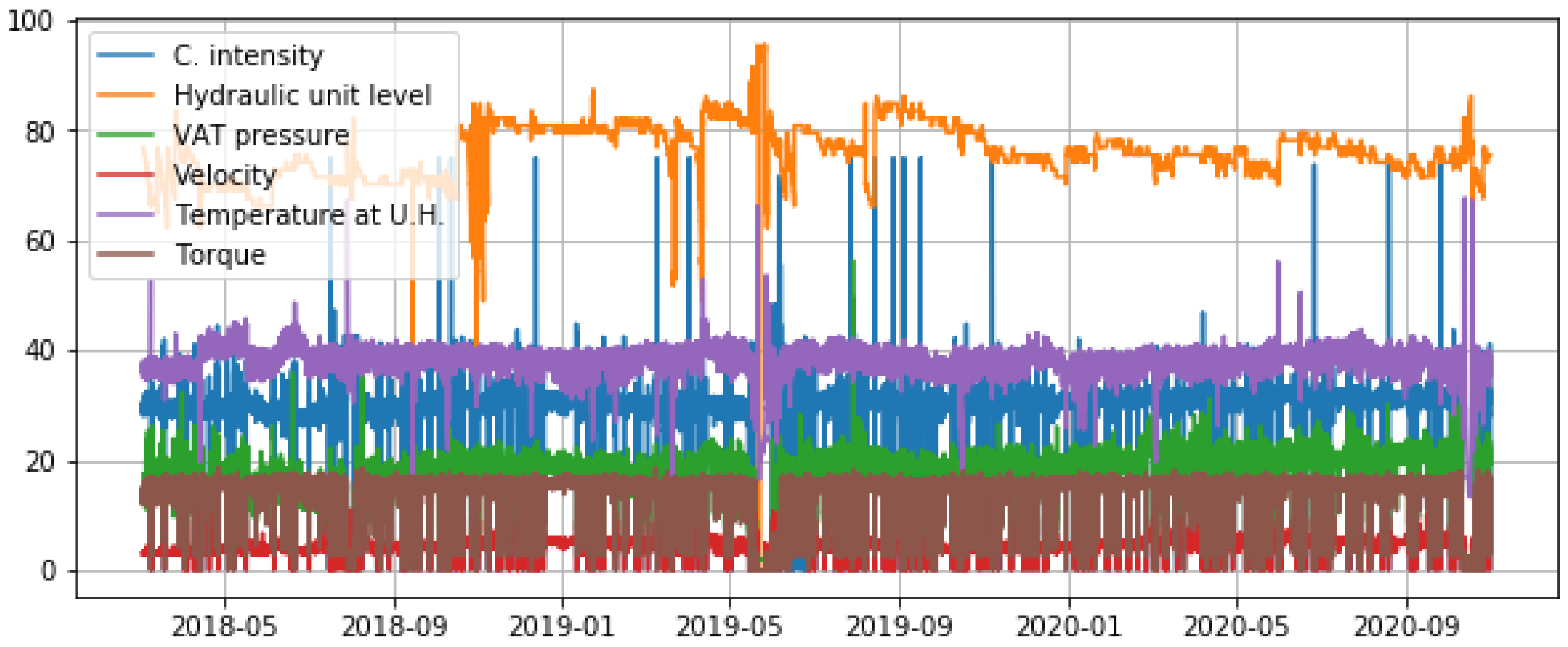
The main goal of the present work is to predict potential failures in an industrial drying press before they happen. Data come from six sensors installed in the press. Those sensors monitor the operation of the press, with a sampling period of one minute. The monitored variables are: (1) electric current intensity; (2) oil level at the hydraulic unit; (3) VAT pressure; (4) rotation speed; (5) temperature in the hydraulic unit; and (6) torque. The dataset contains six time series, one for each sensor, with the values stored in the database from 2016 to August 2020.
Figure 2 shows a plot of the six time series, before any processing is applied. These data present some upper and lower extremes, which may be discrepant data. Those discrepant samples may be due to reading errors or periods when the equipment was off or in another atypical state.
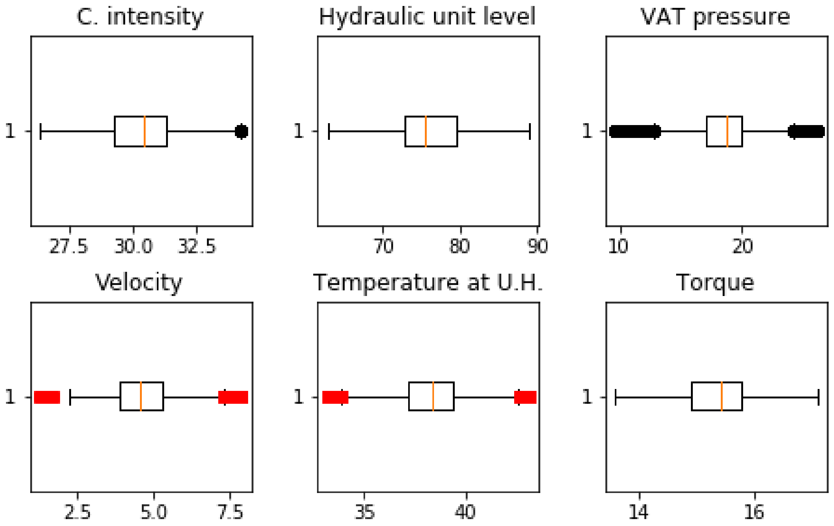
Some of the samples, such as those when the equipment was off but the sensors were still reading, can compromise the training of the machine learning models to be developed. Table 1 shows some statistical parameters such as mean, standard deviation (std), minimum, third quantiles, and maximum value.
4.2. Cleaning Discrepant Data
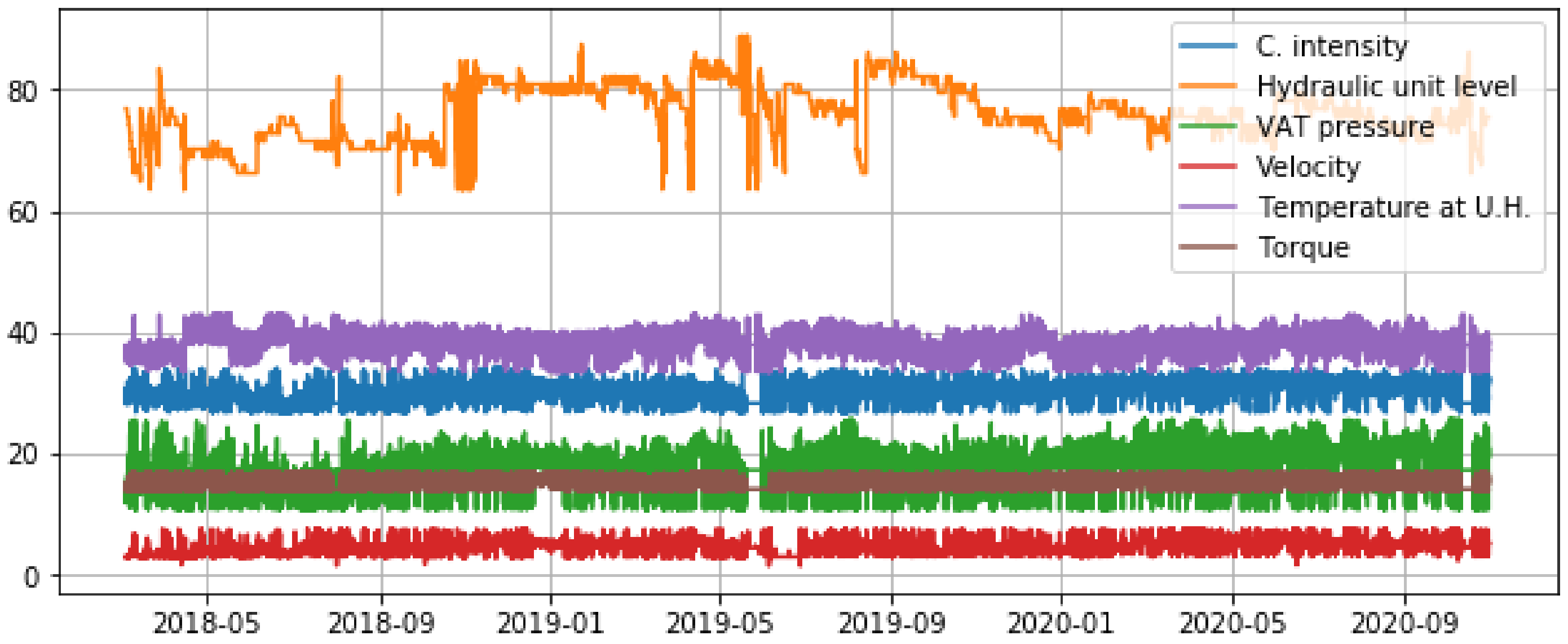
In order to facilitate the training process, discrepant samples were identified and removed using the quantiles method. Samples which are beyond the or are replaced by the mean value. The extreme values were replaced with the average. Figure 3 shows the same variables after discrepant data samples were removed.
As the figure shows, the lines are now smoother and easier to read. Figure 4 shows that the samples are evenly distributed after the withdrawal of discrepant data.
The predictive models to be used are robust and tolerant to noise. However, the cleaner data are expected to show better results. As an example, a provisional experiment to train a neural network LSTM model with a historical window of 70 samples and 40 LSTM unit cells showed higher and undetermined errors. The model was not able to learn or predict some variables, as shown in Table 2. With clean data, there were better and determinable results, as shown in Table 3. The tables show the MAPE and MAE for all input variables, as determined in the test set. They also show the RMSE, as calculated in the train and test sets, globally for all variables.
5. Experiments and Results
Experiments were performed with the aim of validating the model that has the best performance in predicting data from the industrial press. The tests are divided into two subsections, first with resampling of data to one sample per day and then with resampling for a sample each 12 h.
5.1. LSTM Models and Dataset Partition
After processing the data, experiments were performed with an LSTM model. The model included an encoder and decoder, with one hidden LSTM layer in the middle and a dense layer at the output. The model was used to train and predict, with six variables that represent data coming from the paper press sensors. The goal was to forecast the value of those variables with the highest possible level of confidence so that it brings added benefits in predictive maintenance.
Figure 5 describes the architecture of one of the network models used. The models were implemented in Python using the TensorFlow library and Keras.
The experiments were performed aiming to obtain a prediction for all variables one month in advance, from a window of a number of past samples.
The LSTM models received, as an input, a sequence consisting of the composition of a number of samples for each variable. The number of samples depended on the window size and the resampling rate used. The output sequence is composed of the values predicted for each of the variables.
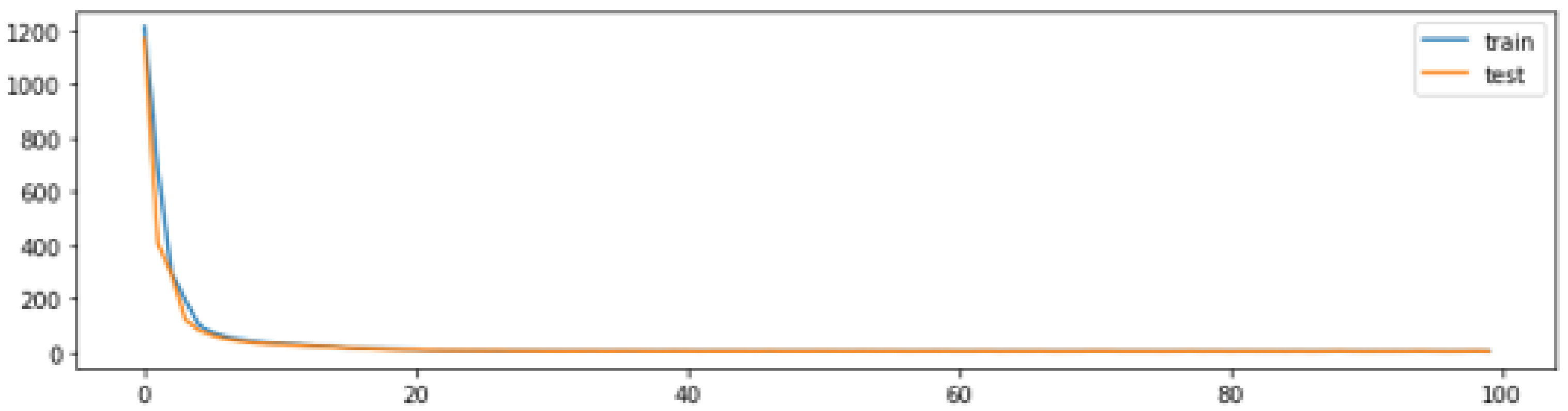
To train and test the models, the dataset was divided into train and test subsets. Validation was performed using the test set, but those samples were not incorporated into the training set. The training set contained 85% of the samples and the test set the remaining 15% of samples. These values are adequate for convergence during learning. As an example, Figure 6 shows a learning curve for a model with 70 units in the middle layer and a window of 30 lag samples. The figure shows that learning converges and takes fewer than 10 epochs. The remainder experiments were performed using 100 epochs.
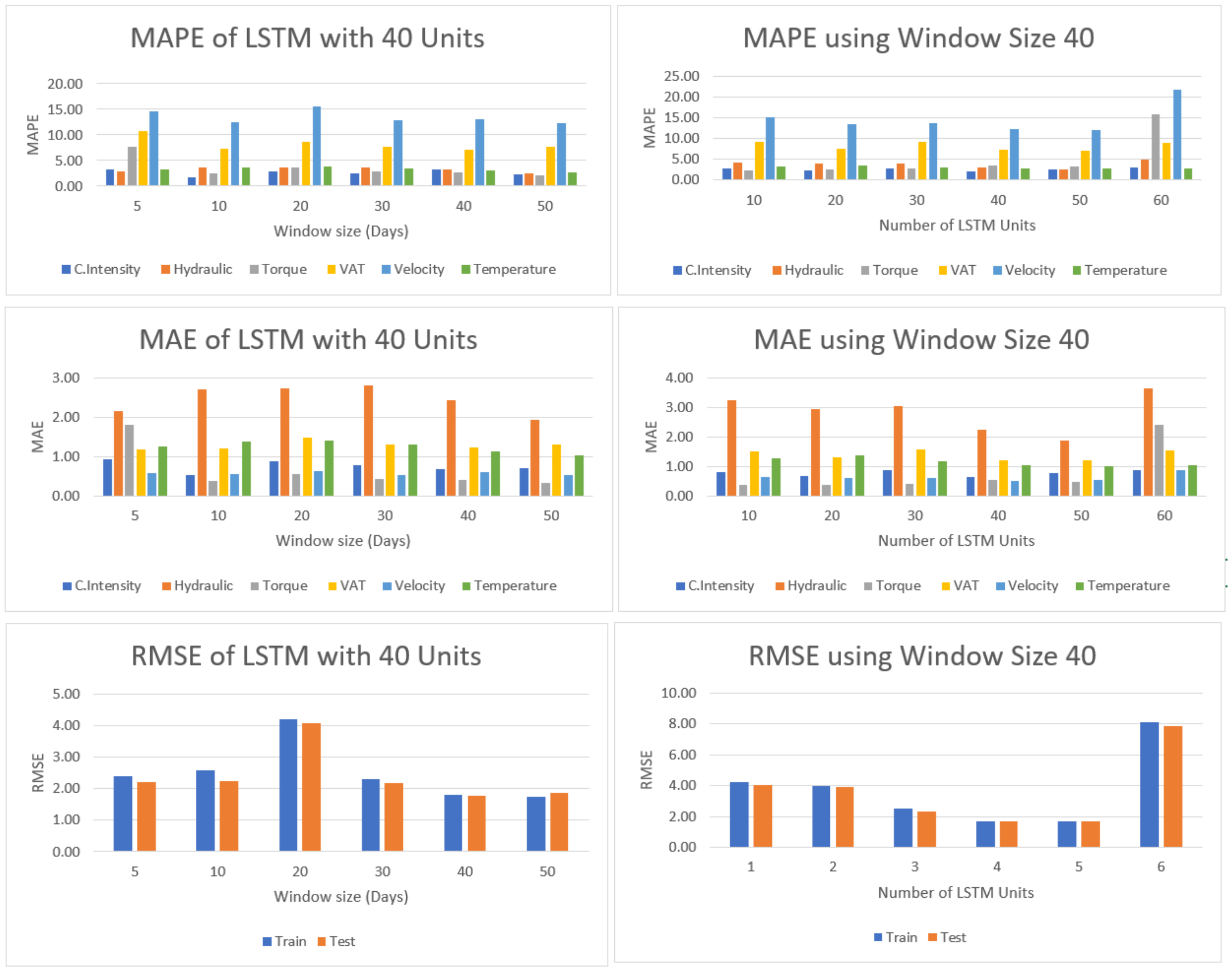
5.2. Experiments to Determine Historical Window Size and Number of LSTM Units Using One Sample per Day
The first experiments performed aimed to determine the best window size to use. The smaller the window, the smaller and faster the model that can be used. However, if the window is too small, it may be insufficient to make accurate predictions.
The original dataset had 1,445,760 data points, which is very large and would require a lot of memory and time to train and test. The experiments were performed after downsampling the data, so that there is only one sample per day. That sample is the average of 1004 original samples. The downsampled dataset is, therefore, less than the one thousand of the original dataset.
The results are measured in the test set. The figure above shows the MAPE and MAE measured for each variable. It also shows the global RMSE measured globally for the train and test sets.
As Figure 7 shows, models with windows of 40 and 50 samples allow better learning and produce smaller prediction errors.
Additional experiments were performed to determine the best size for the number of cells in the hidden layer. For those experiments, a window of 40 historical samples was used, relying on the results of the previous experiments.
Figure 7 shows the results obtained for experiments with a window of 40 days and different numbers of hidden cells. As the results show, the model with the best performance is the one with 50 hidden cells.
After the results of the first experiments with one sample per day, additional experiments were conducted to determine if there was any considerable loss in downsampling from one sample per minute to one sample per day. A first experiment was performed, which consisted of halving the downsampling period from 24 to just 12 h. Therefore, the dataset doubled in size, since it contained two samples per day instead of just one.
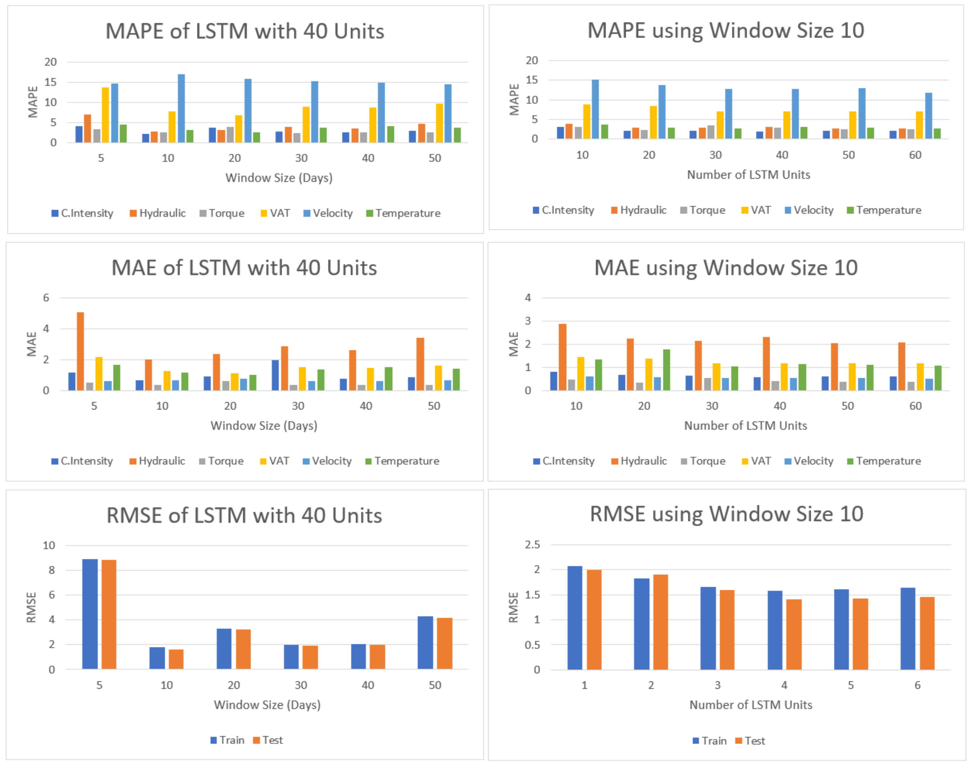
5.3. Experiments to Determine Historical Window Size and Number of Unit LSTMs Using Two Samples per Day
According to the results shown in Figure 8, it is concluded that a window of 10 days (20 samples) shows the best performance. This shows that the model can exhibit approximately the same performance with even fewer input samples when compared to the models above. The models used for those experiments had 20 cells in the hidden layer.
Once the impact of the window size was determined, additional experiments were performed to gain a better insight into the impact of using more or less cells in the hidden layer. Figure 8 shows results of using different numbers of cells.
5.4. Plot of One Result
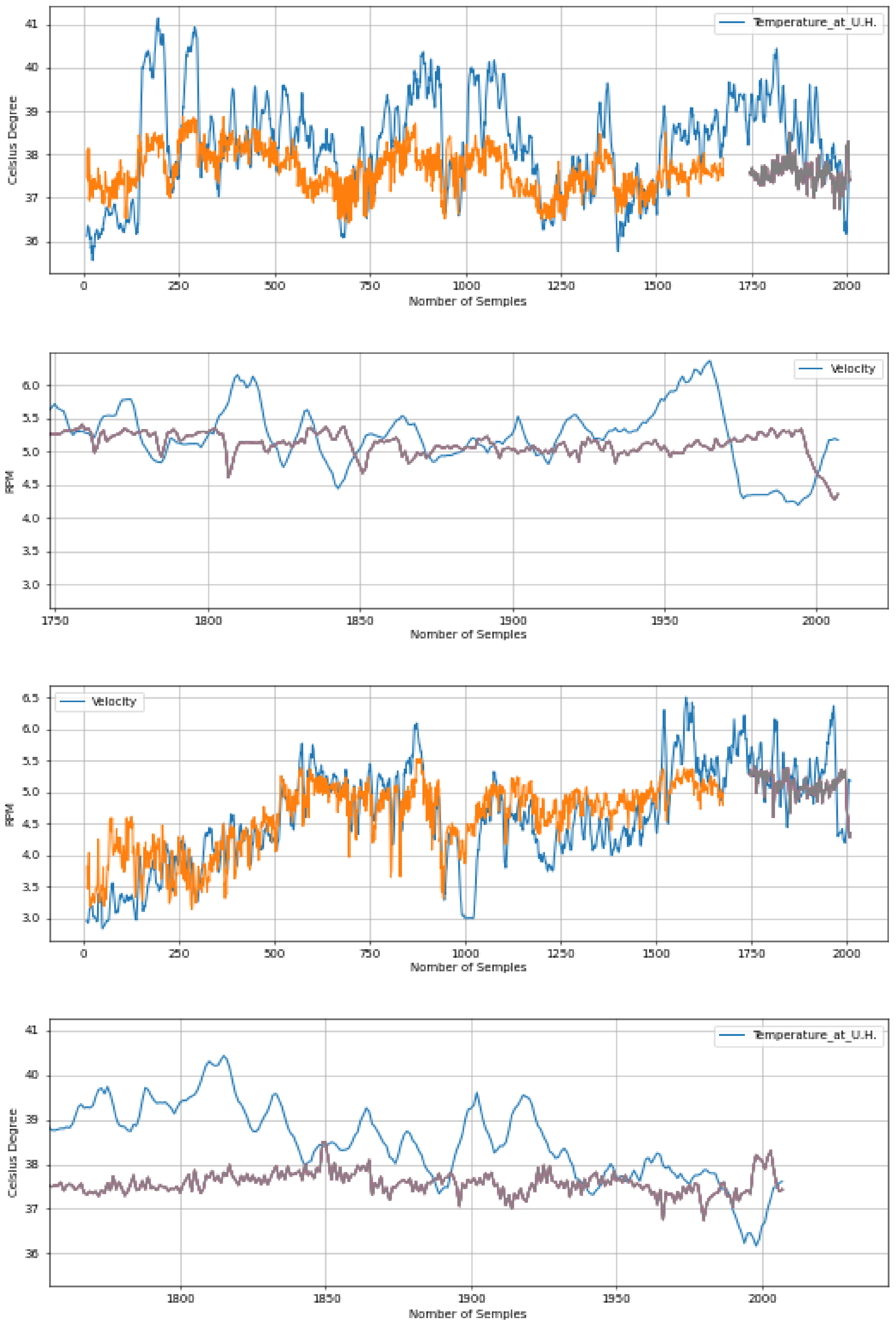
Figure 9 shows plots of the results obtained using the model using 40 units in the hidden layer and a 10-day window of samples. As the figure shows, the forecasts in general follow the actual signals most of the time. However, there are still some areas where the actual signal diverges a small percentage from the prediction, namely for velocity and temperature. Most of the differences may be due to behaviors that are still difficult to capture due to the small dimension of the dataset. As more data will be collected, the neural models will probably be able to capture more patterns and offer more accurate predictions.
6. Discussion
Anticipating industrial equipment’s future behavior is a goal that has been long sought after, for it allows predictive maintenance to perform the right actions at the right time. Therefore, the application of time series and other artificial intelligence models to forecast the equipment’s state is a new and growing area of interest.
The present research uses a dataset of approximately 2.5 years of data of an industrial paper press. A procedure to clean the data is proposed and different experiments are described to use a deep neural model based on LSTM recurrent networks.
The method proposed is going to be applied in other industrial presses, aiming to improve predictive maintenance. Based on the state of the art and experiments, this architecture presents a good versatility, depending of course on the quality of data and hyperparameter settings.
The results show that it is possible to optimize neural models to forecast future values 30 days in advance. The model experimented uses as input a vector consisting of concatenation of a number of samples of all variables. The output is a vector with the predictions of all samples too. The performance of the models is generally better for some variables and worse for others. Those differences will be dealt with in future work.
An important conclusion is that the downsampling used might have been too aggressive. Experiments were performed using one sample per day and two samples per day. The models trained with two samples per day showed a better performance. Hence, more resolution is better for reducing errors and may allow for better learning. That is achieved at the cost of additional processing power. This is also another research question which will be dealt with in future work.
7. Conclusions
Predicting industrial machines’ future behaviors is key for predictive maintenance success. The present research aims to find prediction models adequate for anticipating the future behavior of industrial equipment with good certainty.
The predictive model used was based on LSTM networks, with encoding and decoding layers as the input and output, respectively. In this study, different data pre-processing techniques, network architectures, and hyperparameters were tested, in order to determine the best models.
The predictive model used was based on LSTM network, with encoding and decoding layers as the input and output, respectively.
The results show that the model proposed is able to learn and forecast the behavior of the six variables studied: torque, pressure, current intensity, velocity, oil level and temperature. The best results were obtained using a window of samples of the last 10 days at two samples per day. The MAPE errors varied in the range of 2 to 17% for one of the best models for different variables.
Future work includes additional experiments to determine the optimal sampling rate and stabilize the results for optimal performance with all the variables. The predicted results will also be used to determine an expected probability of failure, using classification models. Other methods may also be used to deal with discrepant data. Later, the models developed will also be applied to other equipment.
Author Contributions
Conceptualization, J.T.F., A.M.C., M.M.; methodology, J.T.F. and M.M.; software, B.C.M. and M.M.; validation, J.T.F. and M.M.; formal analysis, J.T.F. and M.M.; investigation, B.C.M. and M.M.; resources, J.T.F., A.M.C. and M.M.; writing—original draft preparation, B.C.M.; writing—review and editing, J.T.F. and M.M.; project administration, J.T.F. and A.M.C.; funding acquisition, J.T.F. and A.M.C. All authors have read and agreed to the published version of the manuscript.
Funding
The research leading to these results has received funding from the European Union’s Horizon 2020 research and innovation programme under the Marie Sklodowvska-Curie grant agreement 871284 project SSHARE and the European Regional Development Fund (ERDF) through the Operational Programme for Competitiveness and Internationalization (COMPETE 2020), under Project POCI-01-0145-FEDER-029494, and by National Funds through the FCT—Portuguese Foundation for Science and Technology, under Projects PTDC/EEI-EEE/29494/2017, UIDB/04131/2020, and UIDP/04131/2020.
Acknowledgments
This research is sponsored by FEDER funds through the program COMPETE—Programa Operacional Factores de Competitividade—and by national funds through FCT—Fundação para a Ciência e a Tecnologia—under the project UIDB/00285/2020. This work was produced with the support of INCD funded by FCT and FEDER under the project 01/SAICT/2016 nº 022153.
Conflicts of Interest
The authors declare no conflict of interest.
Abbreviations
The following abbreviations are used in this manuscript:
| ARMA | Autoregressive Integrated Moving Average |
| CNN | Convolution Neural Networks |
| LSTM | Long Short-Term Memory |
| MAE | Mean Absolute Error |
| MAPE | Mean Absolute Percentage Error |
| RMSE | Root Mean Square Error |
| RNN | Recurrent Neural Networks |
References
- Sahal, R.; Breslin, J.; Ali, M. Big data and stream processing platforms for Industry 4.0 requirements mapping for a predictive maintenance use case. J. Manuf. Syst. 2020, 54, 138–151. [Google Scholar] [CrossRef]
- Ahmed, M.S.; Cook, A.R. Analysis of Freeway Traffic Time-Series Data by Using Box-Jenkins Techniques; Transportation Research Board: Washington, DC, USA, 2020; ISBN 9780309029728. [Google Scholar]
- Majeed, A.; Zhang, Y.; Ren, S.; Lv, J.; Peng, T.; Waqar, S.; Yin, E. A big data-driven framework for sustainable and smart additive manufacturing. Robot. Comput. Integr. Manuf. 2021, 67, 102026. [Google Scholar] [CrossRef]
- Ferreiro, S.; Konde, E.; Fernández, S.; Prado, A. Industry 4.0: Predictive intelligent maintenance for production equipment. In European Conference of the Prognostics and Health Management Society; 2016; pp. 1–8. Available online: https://www.semanticscholar.org/paper/INDUSTRY-4-.-0-%3A-Predictive-Intelligent-Maintenance-Ferreiro-Konde/638c2b72a747ea4b82e098572be820083dca9c7a (accessed on 25 June 2021).
- Wang, K. Intelligent predictive maintenance (IPdM) system—Industry 4.0 scenario. WIT Trans. Eng. Sci. 2016, 113, 259–268. [Google Scholar]
- Yu, W.; Dillon, T.; Mostafa, F.; Rahayu, W.; Liu, Y. A global manufacturing big data ecosystem for fault detection in predictive maintenance. IEEE Trans. Ind. Inform. 2020, 16, 183–192. [Google Scholar] [CrossRef]
- Pais, E.; Farinha, J.T.; Cardoso, A.J.M.; Raposo, H. Optimizing the Life Cycle of Physical Assets—A Review. WSEAS Trans. Syst. Control 2020, 15, 417–430. [Google Scholar] [CrossRef]
- Martins, A.B.; Torres Farinha, J.; Marques Cardoso, A. Calibration and Certification of Industrial Sensors—A Global Review. WSEAS Trans. Syst. Control 2020, 15, 394–416. [Google Scholar] [CrossRef]
- Rodrigues, J.; Cost, I.; Farinha, J.; Mendes, M.; Margalho, L. Predicting motor oil condition using artificial neural networks and principal component analysis. Eksploat. Niezawodn. 2020, 22, 440–448. [Google Scholar] [CrossRef]
- Torres Farinha, J. Asset Maintenance Engineering Methodologies; CRC Press: Boca Raton, FL, USA, 2018. [Google Scholar]
- Chen, M.; Tseng, H. An approach to design of maintenance float systems. Integr. Manuf. 2003, 14, 458–467. [Google Scholar]
- Daniyan, I.; Mpofu, K.; Oyesola, M.; Ramatsetse, B.; Adeodu, A. Artificial intelligence for predictive maintenance in the railcar learning factories. Procedia Manuf. 2020, 45, 13–18. [Google Scholar] [CrossRef]
- Hsu, Y.Y.; Tung, T.T.; Yeh, H.C.; Lu, C.N. Two-Stage Artificial Neural Network Model for Short-Term Load Forecasting. IFAC-PapersOnLine 2018, 51, 678–683. [Google Scholar] [CrossRef]
- Balduíno, M.; Torres Farinha, J.; Marques Cardoso, A. Production Optimization versus Asset Availability—A Review. WSEAS Trans. Syst. Control 2020, 15, 320–332. [Google Scholar] [CrossRef]
- Jimenez, V.J.; Bouhmala, N.; Gausdal, A.H. Developing a predictive maintenance model for vessel machinery. J. Ocean. Eng. Sci. 2020, 5, 358–386. [Google Scholar] [CrossRef]
- Ayvaz, S.; Alpay, K. Predictive maintenance system for production lines in manufacturing: A machine learning approach using IoT data in real-time. Expert Syst. Appl. 2021, 173, 114598. [Google Scholar] [CrossRef]
- Yu, Z.; Moirangthem, D.S.; Lee, M. Continuous Timescale Long-Short Term Memory Neural Network for Human Intent Understanding. Front. Neurorobot. 2017, 11, 42. [Google Scholar] [CrossRef]
- Aydin, O.; Guldamlasioglu, S. Using LSTM networks to predict engine condition on large scale data processing framework. In Proceedings of the 2017 4th International Conference on Electrical and Electronic Engineering (ICEEE), Ankara, Turkey, 8–10 April 2017; pp. 281–285. [Google Scholar] [CrossRef]
- Wang, Q.; Bu, S.; He, Z. Achieving Predictive and Proactive Maintenance for High-Speed Railway Power Equipment with LSTM-RNN. IEEE Trans. Ind. Inform. 2020, 16, 6509–6517. [Google Scholar] [CrossRef]
- Bruneo, D.; De Vita, F. On the Use of LSTM Networks for Predictive Maintenance in Smart Industries. In Proceedings of the 2019 IEEE International Conference on Smart Computing (SMARTCOMP), Washington, DC, USA, 12–15 June 2019; pp. 241–248. [Google Scholar] [CrossRef]
- Dong, D.; Li, X.Y.; Sun, F.Q. Life prediction of jet engines based on LSTM-recurrent neural networks. In Proceedings of the 2017 Prognostics and System Health Management Conference (PHM-Harbin), Harbin, China, 9–12 July 2017; pp. 1–6. [Google Scholar] [CrossRef]
- Bampoula, X.; Siaterlis, G.; Nikolakis, N.; Alexopoulos, K. A Deep Learning Model for Predictive Maintenance in Cyber-Physical Production Systems Using LSTM Autoencoders. Sensors 2021, 21, 972. [Google Scholar] [CrossRef]
- Mathew, V.; Toby, T.; Singh, V.; Rao, B.M.; Kumar, M.G. Prediction of Remaining Useful Lifetime (RUL) of turbofan engine using machine learning. In Proceedings of the 2017 IEEE International Conference on Circuits and Systems (ICCS), Thiruvananthapuram, India, 20–21 December 2017; pp. 306–311. [Google Scholar] [CrossRef]
- Düdükçü, H.V.; Taşkıran, M.; Kahraman, N. LSTM and WaveNet Implementation for Predictive Maintenance of Turbofan Engines. In Proceedings of the 2020 IEEE 20th International Symposium on Computational Intelligence and Informatics (CINTI), Budapest, Hungary, 5–7 November 2020; pp. 151–156. [Google Scholar] [CrossRef]
- Essien, A.; Giannetti, C. A Deep Learning Model for Smart Manufacturing Using Convolutional LSTM Neural Network Autoencoders. IEEE Trans. Ind. Inform. 2020, 16, 6069–6078. [Google Scholar] [CrossRef] [Green Version]
- Schmidhuber, J. Deep learning in neural networks: An overview. Neural Netw. 2015, 61, 85–117. [Google Scholar] [CrossRef] [Green Version]
- Beshr, A.; Zarzoura, F. Using artificial neural networks for GNSS observations analysis and displacement prediction of suspension highway bridge. Innov. Infrastruct. Solut. 2021, 6. [Google Scholar] [CrossRef]
- Sak, H.; Senior, A.; Beaufays, F. Long Short-Term Memory Based Recurrent Neural Network Architectures for Large Vocabulary Speech Recognition. arXiv 2014, arXiv:1402.1128. [Google Scholar]
- Chen, Z.; Liu, Y.; Liu, S. Mechanical state prediction based on LSTM neural netwok. In Proceedings of the 2017 36th Chinese Control Conference (CCC), Dalian, China, 26–28 July 2017; pp. 3876–3881. [Google Scholar] [CrossRef]
- Ghosh, S.; Vinyals, O.; Strope, B.; Roy, S.; Dean, T.; Heck, L. Contextual LSTM (CLSTM) models for Large scale NLP tasks. arXiv 2016, arXiv:1602.06291. [Google Scholar]
- Shahid, F.; Zameer, A.; Muneeb, M. A novel genetic LSTM model for wind power forecast. Energy 2021, 223, 120069. [Google Scholar] [CrossRef]
- Guo, J.; Xie, Z.; Qin, Y.; Jia, L.; Wang, Y. Short-Term Abnormal Passenger Flow Prediction Based on the Fusion of SVR and LSTM. IEEE Access 2019, 7, 42946–42955. [Google Scholar] [CrossRef]
- Ren, L.; Dong, J.; Wang, X.; Meng, Z.; Zhao, L.; Deen, M. A Data-Driven Auto-CNN-LSTM Prediction Model for Lithium-Ion Battery Remaining Useful Life. IEEE Trans. Ind. Inform. 2021, 17, 3478–3487. [Google Scholar] [CrossRef]
- Niu, K.; Zhang, H.; Zhou, T.; Cheng, C.; Wang, C. A Novel Spatio-Temporal Model for City-Scale Traffic Speed Prediction. IEEE Access 2019, 7, 30050–30057. [Google Scholar] [CrossRef]
- Feng, M.; Zheng, J.; Ren, J.; Hussain, A.; Li, X.; Xi, Y.; Liu, Q. Big Data Analytics and Mining for Effective Visualization and Trends Forecasting of Crime Data. IEEE Access 2019, 7, 106111–106123. [Google Scholar] [CrossRef]
- Palangi, H.; Deng, L.; Shen, Y.; Gao, J.; He, X.; Chen, J.; Song, X.; Ward, R. Deep Sentence Embedding Using Long Short-Term Memory Networks: Analysis and Application to Information Retrieval. IEEE/ACM Trans. Audio Speech Lang. Process. 2016, 24, 694–707. [Google Scholar] [CrossRef] [Green Version]
- Rumelhart, D.E.; Hinton, G.E.; Williams, R.J. Learning representations by back-propagating errors. Nature 1986, 323, 533–536. [Google Scholar] [CrossRef]
- Mao, Y.; Qin, G.; Ni, P.; Liu, Q. Analysis of road traffic speed in Kunming plateau mountains: A fusion PSO-LSTM algorithm. Int. J. Urban Sci. 2021, 1–21. [Google Scholar] [CrossRef]
- Hutter, F.; Lücke, J.; Schmidt-Thieme, L. Beyond Manual Tuning of Hyperparameters. KI Künstliche Intell. 2015, 29, 329–337. [Google Scholar] [CrossRef]
- Khalid, R.; Javaid, N. A survey on hyperparameters optimization algorithms of forecasting models in smart grid. Sustain. Cities Soc. 2020, 61, 102275. [Google Scholar] [CrossRef]
- Hutter, F.; Hoos, H.; Leyton-Brown, K. An Efficient Approach for Assessing Hyperparameter Importance. In Proceedings of the 31st International Conference on Machine Learning, Beijing, China, 21–26 June 2014; pp. 754–762. [Google Scholar]
- Park, S.H.; Kim, B.; Kang, C.M.; Chung, C.C.; Choi, J.W. Sequence-to-Sequence Prediction of Vehicle Trajectory via LSTM Encoder-Decoder Architecture. In Proceedings of the 2018 IEEE Intelligent Vehicles Symposium (IV), Changshu, China, 26–30 June 2018; pp. 1672–1678. [Google Scholar] [CrossRef] [Green Version]
- Cho, K.; van Merrienboer, B.; Gülçehre, Ç.; Bougares, F.; Schwenk, H.; Bengio, Y. Learning Phrase Representations using RNN Encoder-Decoder for Statistical Machine Translation. arXiv 2014, arXiv:1406.1078. [Google Scholar]
- Sutskever, I.; Vinyals, O.; Le, Q.V. Sequence to Sequence Learning with Neural Networks. arXiv 2014, arXiv:1409.3215. [Google Scholar]
- Wang, T.; Chen, P.; Amaral, K.; Qiang, J. An Experimental Study of LSTM Encoder-Decoder Model for Text Simplification. arXiv 2016, arXiv:1609.03663. [Google Scholar]
- Bengio, S.; Vinyals, O.; Jaitly, N.; Shazeer, N. Scheduled Sampling for Sequence Prediction with Recurrent Neural Networks. arXiv 2015, arXiv:1506.03099. [Google Scholar]
- Du, S.; Li, T.; Yang, Y.; Horng, S.J. Multivariate time series forecasting via attention-based encoder–decoder framework. Neurocomputing 2020, 388, 269–279. [Google Scholar] [CrossRef]
- Gers, F.A.; Eck, D.; Schmidhuber, J. Applying LSTM to Time Series Predictable Through Time-Window Approaches. In Neural Nets WIRN Vietri-01; Perspectives in Neural Computing; Tagliaferri, R., Marinaro, M., Eds.; Springer: Berlin/Heidelberg, Germany, 2002; pp. 193–200. [Google Scholar] [CrossRef]
- Meng, Q.; Wang, H.; He, M.; Gu, J.; Qi, J.; Yang, L. Displacement prediction of water-induced landslides using a recurrent deep learning model. Eur. J. Environ. Civ. Eng. 2020. [Google Scholar] [CrossRef]
- Sarikaya, R.; Hinton, G.E.; Deoras, A. Application of Deep Belief Networks for Natural Language Understanding. IEEE/ACM Trans. Audio Speech Lang. Process. 2014, 22, 778–784. [Google Scholar] [CrossRef] [Green Version]
- Sundermeyer, M.; Schlüter, R.; Ney, H. LSTM neural networks for language modeling. In Proceedings of the Thirteenth Annual Conference of the International Speech Communication Association, Portland, OR, USA, 9–13 September 2012. [Google Scholar]
- Hu, Y.; Sun, X.; Nie, X.; Li, Y.; Liu, L. An Enhanced LSTM for Trend Following of Time Series. IEEE Access 2019, 7, 34020–34030. [Google Scholar] [CrossRef]
- Gers, F.A.; Schmidhuber, J.; Cummins, F. Learning to Forget: Continual Prediction with LSTM. In Proceedings of the 1999 Ninth International Conference on Artificial Neural Networks ICANN 99 (Conf. Publ. No. 470), Edinburgh, UK, 7–10 September 1999; pp. 850–855. [Google Scholar] [CrossRef]
- Greff, K.; Srivastava, R.K.; Koutník, J.; Steunebrink, B.R.; Schmidhuber, J. LSTM: A Search Space Odyssey. IEEE Trans. Neural Netw. Learn. Syst. 2017, 28, 2222–2232. [Google Scholar] [CrossRef] [PubMed] [Green Version]
- Hochreiter, S.; Schmidhuber, J. Long Short-Term Memory. Neural Comput. 1997, 9, 1735–1780. [Google Scholar] [CrossRef] [PubMed]
- Li, C.; Jiang, P.; Zhou, A. Rigorous solution of slope stability under seismic action. Comput. Geotech. 2019, 109, 99–107. [Google Scholar] [CrossRef]
- Li, C.; Hu, B.C.; Hu, D.; Xu, X.F.; Zong, X.C.; Li, J.P.; Wu, M.C. Stereoselective ring-opening of styrene oxide at elevated concentration by Phaseolus vulgaris epoxide hydrolase, PvEH2, in the organic/aqueous biphasic system. Catal. Commun. 2019, 123, 1–5. [Google Scholar] [CrossRef]
- Qin, Y.; Li, K.; Liang, Z.; Lee, B.; Zhang, F.; Gu, Y.; Zhang, L.; Wu, F.; Rodriguez, D. Hybrid forecasting model based on long short term memory network and deep learning neural network for wind signal. Appl. Energy 2019, 236, 262–272. [Google Scholar] [CrossRef]
- Zhang, Z.; Ye, L.; Qin, H.; Liu, Y.; Wang, C.; Yu, X.; Yin, X.; Li, J. Wind speed prediction method using Shared Weight Long Short-Term Memory Network and Gaussian Process Regression. Appl. Energy 2019, 247, 270–284. [Google Scholar] [CrossRef]
- Zhao, R.; Yin, Y.; Shi, Y.; Xue, Z. Intelligent intrusion detection based on federated learning aided long short-term memory. Phys. Commun. 2020, 42, 101157. [Google Scholar] [CrossRef]
- Kong, X.; Kong, D.; Bai, L.; Xiao, J. Online pricing of demand response based on long short-term memory and reinforcement learning. Appl. Energy 2020, 271, 114945. [Google Scholar] [CrossRef]
- Li, Y.; Lu, Y. LSTM-BA: DDoS Detection Approach Combining LSTM and Bayes. In Proceedings of the 2019 Seventh International Conference on Advanced Cloud and Big Data (CBD), Suzhou, China, 21–22 September 2019; pp. 180–185. [Google Scholar] [CrossRef]
- Alameer, Z.; Fathalla, A.; Li, K.; Ye, H.; Jianhua, Z. Multistep-ahead forecasting of coal prices using a hybrid deep learning model. Resour. Policy 2020, 65, 101588. [Google Scholar] [CrossRef]
Figure 1.
Detailed layout of a long short-term memory unit [63].
Figure 1.
Detailed layout of a long short-term memory unit [63].

Figure 2.
Plot of the original dataset values. The variables are electric current intensity, hydraulic unit oil level, VAT pressure, motor velocity, temperature at the hydraulic unit, and torque.
Figure 2.
Plot of the original dataset values. The variables are electric current intensity, hydraulic unit oil level, VAT pressure, motor velocity, temperature at the hydraulic unit, and torque.

Figure 3.
Plot of the dataset values after cleaning discrepant data. The variables are current intensity, hydraulic unit oil level, VAT pressure, velocity, temperature, and torque.
Figure 3.
Plot of the dataset values after cleaning discrepant data. The variables are current intensity, hydraulic unit oil level, VAT pressure, velocity, temperature, and torque.

Figure 4.
Distribution of data points of all the sensors, with lowly and highly discrepant data cleaned.
Figure 4.
Distribution of data points of all the sensors, with lowly and highly discrepant data cleaned.

Figure 5.
Model summary of one of the LSTM networks used. The model receives a window of n samples of each variable and predicts the value of those variables as predicted 30 days ahead.
Figure 5.
Model summary of one of the LSTM networks used. The model receives a window of n samples of each variable and predicts the value of those variables as predicted 30 days ahead.

Figure 6.
Example of learning curve, showing the loss measured during training of an LSTM model.

Figure 7.
Results obtained with a different number of LSTM cells in the hidden layer, as well as different sliding window sizes, to predict values 30 days in advance with downsampling to one sample per day.
Figure 7.
Results obtained with a different number of LSTM cells in the hidden layer, as well as different sliding window sizes, to predict values 30 days in advance with downsampling to one sample per day.

Figure 8.
Results obtained with a different number of cells in the hidden layer, also using different window samples to predict values 30 days in advance with resampling for the two samples for a day.
Figure 8.
Results obtained with a different number of cells in the hidden layer, also using different window samples to predict values 30 days in advance with resampling for the two samples for a day.

Figure 9.
Variable forecast with a window of samples of 10 days, sampling rate two samples per day, and a network model with 50 units in the hidden layer. The blue lines show the actual value. The orange lines show the predictions during the training set and the gray lines show the predictions in the test set.


Table 1.
Statistical parameters of the dataset variables, before processing: C. intensity, hydraulic unit oil level, torque, VAT pressure, velocity, and temperature.
Table 1.
Statistical parameters of the dataset variables, before processing: C. intensity, hydraulic unit oil level, torque, VAT pressure, velocity, and temperature.
| C. Intensity | Hydraulic | Torque | VAT | Velocity | Temperature | |
|---|---|---|---|---|---|---|
| mean | 30.26 | 75.90 | 15.28 | 18.25 | 4.59 | 38.22 |
| std | 1.36 | 4.54 | 0.69 | 2.67 | 0.98 | 1.62 |
| min | 26.34 | 62.93 | 13.59 | 9.67 | 1.27 | 33.19 |
| —25% | 29.30 | 72.86 | 14.90 | 17.13 | 3.92 | 37.17 |
| —50% | 30.46 | 75.53 | 15.43 | 18.72 | 4.57 | 38.33 |
| —75% | 31.28 | 79.52 | 15.78 | 19.97 | 5.28 | 39.35 |
| max | 34.26 | 88.97 | 17.09 | 26.17 | 7.87 | 43.10 |
Table 2.
Prediction results without cleaning discrepant data in the database, with a window of 70 samples and 40 LSTM units.
Table 2.
Prediction results without cleaning discrepant data in the database, with a window of 70 samples and 40 LSTM units.
| Window 70 Days | ||||||
|---|---|---|---|---|---|---|
| C. Intensity | Hydraulic | Torque | VAT | Velocity | Temperature | |
| MAPE | inf | 8.46 | inf | 98.19 | inf | 11.59 |
| MAE | 3.52 | 6.57 | 24.73 | 10.53 | 14.88 | 4.21 |
| Train | Test | |||||
| RMSE | 79.52 | 79.64 | ||||
Table 3.
Forecast results with treatments in the database with 40 LSTM units.
| Window 70 Days | ||||||
|---|---|---|---|---|---|---|
| C. Intensity | Hydraulic | Torque | VAT | Velocity | Temperature | |
| MAPE | 2.52 | 3.02 | 2.44 | 13.10 | inf | 2.48 |
| MAE | 0.76 | 2.28 | 0.37 | 1.32 | 0.57 | 0.94 |
| Train | Test | |||||
| RMSE | 1.71 | 1.97 | ||||
Table 4.
The magnitude of RMSE errors in the test and training set, using one sample per day.
| Window Size (Days) | Train | Test | Units | Train | Test |
|---|---|---|---|---|---|
| 5 | 2.39 | 2.20 | 10 | 4.23 | 4.07 |
| 10 | 2.57 | 2.24 | 20 | 3.99 | 3.93 |
| 20 | 4.21 | 4.09 | 30 | 2.52 | 2.35 |
| 30 | 2.31 | 2.19 | 40 | 1.68 | 1.70 |
| 40 | 1.81 | 1.77 | 50 | 1.66 | 1.70 |
| 50 | 1.74 | 1.86 | 60 | 8.14 | 7.85 |
Table 5.
The magnitude of RMSE errors in the test and training set, using two samples per day.
| Window Size (Days) | Train | Test | Units | Train | Test |
|---|---|---|---|---|---|
| 5 | 8.91 | 8.87 | 10 | 2.07 | 1.99 |
| 10 | 1.80 | 1.61 | 20 | 1.82 | 1.91 |
| 20 | 3.29 | 3.23 | 30 | 1.65 | 1.59 |
| 30 | 1.98 | 1.94 | 40 | 1.58 | 1.41 |
| 40 | 2.07 | 1.98 | 50 | 1.61 | 1.42 |
| 50 | 4.32 | 4.16 | 60 | 1.64 | 1.46 |
Publisher’s Note: MDPI stays neutral with regard to jurisdictional claims in published maps and institutional affiliations. |
© 2021 by the authors. Licensee MDPI, Basel, Switzerland. This article is an open access article distributed under the terms and conditions of the Creative Commons Attribution (CC BY) license (https://creativecommons.org/licenses/by/4.0/).
Share and Cite
MDPI and ACS Style
Mateus, B.C.; Mendes, M.; Farinha, J.T.; Cardoso, A.M. Anticipating Future Behavior of an Industrial Press Using LSTM Networks. Appl. Sci. 2021, 11, 6101. https://doi.org/10.3390/app11136101
AMA Style
Mateus BC, Mendes M, Farinha JT, Cardoso AM. Anticipating Future Behavior of an Industrial Press Using LSTM Networks. Applied Sciences. 2021; 11(13):6101. https://doi.org/10.3390/app11136101
Chicago/Turabian StyleMateus, Balduíno César, Mateus Mendes, José Torres Farinha, and António Marques Cardoso. 2021. "Anticipating Future Behavior of an Industrial Press Using LSTM Networks" Applied Sciences 11, no. 13: 6101. https://doi.org/10.3390/app11136101
Note that from the first issue of 2016, this journal uses article numbers instead of page numbers. See further details here.