Underwater Image Mosaic Algorithm Based on Improved Image Registration

Abstract

In order to obtain panoramic images in a low contrast underwater environment, an underwater panoramic image mosaic algorithm based on image enhancement and improved image registration (IIR) was proposed. Firstly, mixed filtering and sigma filtering are used to enhance the contrast of the original image and de-noise the image. Secondly, scale-invariant feature transform (SIFT) is used to detect image feature points. Then, the proposed IIR algorithm is applied to image registration to improve the matching accuracy and reduce the matching time. Finally, the weighted smoothing method is used for image fusion to avoid image seams. The results show that IIR algorithm can effectively improve the registration accuracy, shorten the registration time, and improve the image fusion effect. In the field of cruise research, instruments equipped with imaging systems, such as television capture and deep-drag camera systems, can produce a large number of image or video recordings. This algorithm provides support for fast and accurate underwater image mosaic and has important practical significance.

1. Introduction

With the rapid development of image processing technology, image mosaic has become a hot topic in the field of image processing, which refers to combining multiple images with overlapping parts into a panoramic image that mainly consists of image registration and image fusion. In the study of image registration, Hines et al. [1] proposed a method of phase correlation in 1975 using Fourier transformation to effectively register images with translation. However, when the image gets larger, the time of the Fourier transformation increases exponentially, which seriously reduces the efficiency of the algorithm. In 1988, Harris et al. [2] proposed a feature-based registration algorithm that improved the matching speed and accuracy compared with the method of phase correlation, but the calculation of the Harris response function was related to the empirical value and lacked stability. In 2004, Lowe et al. [3] proposed a new image registration algorithm based on scale-invariant feature transform (SIFT). This algorithm applies to images with translation, rotation, and distortion, and its stability is greatly improved. However, it is difficult to avoid many false matching points, and the execution speed of the algorithm is slow. In 2006, Edward et al. [4] proposed an algorithm called features from accelerated segment test (FAST), which significantly improved the detection speed but lacked a description of the feature points. In the same year, Bay et al. [5] proposed the speed-up robust features (SURF) algorithm, which solved the disadvantages of SIFT, but its stability and number of feature points were inferior to SIFT. Then, Michael et al. [6] proposed an improved algorithm based on FAST, named oriented FAST, and Rotated BRIEF (ORB). Moreover, the advantage of this algorithm was that it had a significant increase in noise resistance and speed, but it lacked scale-invariance. Accuracy, rapidity, and stability are three important evaluation indexes in the study of image registration [7].

In terms of the purification of matching point pairs, Liu et al. [8] eliminated some mismatching points by modifying the threshold values of Euclidean distance and integral images, and realized the effective utilization of feature points, but the registration accuracy was still not high. Zhu et al. [9] proposed an improved SIFT algorithm based on the idea of block matching, which had a good registration effect for remote sensing images. To solve the problem of algorithm stability, Yi et al. [10] proposed an iterative SIFT algorithm based on adaptive non-maximum suppression, which realized the high robustness of UAV cognitive navigation but also increased its complexity. Aimed at the problem of poor registration effect caused by simply improving SIFT, scholars started to combine SIFT and the random sample consensus (RANSAC) algorithm for image registration, which was famous for its robustness. Even if there are a few wrong data points, it can still obtain an ideal model parameter.

Rahul et al. [11] presented a comprehensive overview of existing research in RANSAC-based robust estimation, and provided a universal framework for RANSAC (USAC) algorithm. Shi et al. [12] presented an improved RANSAC (I-RANSAC) algorithm for SIFT feature point matching. Li et al. [13] proposed an algorithm based on a double-column histogram, which has a good application in remote sensing images. Zhao et al. [14] proposed an algorithm based on the consistency principle of matching distance and realized high matching accuracy. Eduardo et al. [15] proposed a dynamic distributed robust RANSAC algorithm, which improved the stability index. Gao et al. [16] proposed a rotating average pipeline based on layered RANSAC to handle relative rotational outliers, and improve the accuracy index. Lati et al. [17] proposed an image mosaic algorithm based on effective blur technology, which has good recognition performance for motion blur images. In terms of image fusion, classical fusion algorithms include direct fusion, weighted smooth fusion, PCA fusion, wavelet transformation fusion, and multi-scale transformation fusion [18]. The traditional RANSAC method has obvious disadvantages, because it only produces reasonable results under certain probability, and improves the accuracy through multiple iterations of the optimal solution of model parameters, which increases the complexity of the algorithm.

In addition, in terms of underwater image mosaic, Chen et al. [19] scombined SIFT and wavelet transformation, but the image registration speed was slow. Xie et al. [20] applied the SURF algorithm to underwater images and obtained a good mosaic effect, but only for images of shallow water with good illumination. Rahul et al. [21] proposed a seamless underwater image mosaic technology based on alpha clipping. Due to degradation problems such as low contrast and color deviation of underwater images, traditional image mosaic algorithms cannot be directly applied to underwater image mosaic.

In the above-mentioned studies, there exist three problems. Firstly, the algorithms have high computational complexity. Secondly, the algorithms focus on improving the effectiveness of a single index and less on improving the performance of two or three indicators. Thirdly, they are seldom used for low contrast and low definition in image processing. Based on these problems, in this paper, we proposed an improved image registration (IIR) algorithm to realize the rapidity of calculation and accuracy of image processing, by optimizing the solution of the Homography matrix according to the number of inner points. In addition, the proposed algorithm was tested on the images from the Oxford Buildings Dataset [22] to verify that it has high feasibility since this dataset is recognized by the academic community for image processing research and is highly representative, containing thousands of images. Finally, the IIR algorithm was implemented in underwater image processing to improve the quality of underwater image mosaic.

2. Materials and Methods

2.1. Method of Image Enhancement

2.1.1. Mixed Method for Image Contrast Enhancement

Due to the influence of the complex underwater environment, the underwater images have different degrees of degradation, resulting in low contrast of the original image performance, which directly affects the subsequent image registration and image fusion. The method of piecewise linear transformation is actually to enhance the contrast of various parts of the original image [23]. It enhances the gray area of interest in the image and suppresses that of no interest.

$$l_{out}=\left\{\begin{array}{ll}0\hfill & l_{inp}<l_{\min }\hfill \\ 255\times \left(\frac{l_{inp} - l_{\min }}{l_{\max } - l_{\min }}\right)\hfill & l_{\min }\le l_{inp}\le l_{\max }\hfill \\ 255\hfill & l_{inp}>l_{\max }\hfill \end{array}\right.$$

(1)

In Equation (1), $l_{inp}$ is the pixel value of the input pixel, $l_{out}$ is the pixel value of the output pixel, $l_{\min }$ is the set minimum pixel threshold, $l_{\max }$ is the set maximum threshold of the pixel, and the maximum grayscale value of the pixel is 255. The piecewise linear method is simple and produces very good results, but is not effective for areas that contain a lot of darkness or light.

The method of histogram equalization is adopted to map the pixel gray level and stretch the image nonlinearly [24,25,26,27,28], and thus the probability density of the transformed image gray level is evenly distributed and the overall contrast of the image is improved. In two-dimensional image space, it is assumed that $r$ and $s$ are the gray level of the image before and after transformation, respectively, and the probability density of $r$ is $p(r)$. Then, for the gray level $r_k$, the corresponding probability density after transformation is $S_k$ as follows:

$$s_k={\displaystyle \sum _{c=0}^{k}p(r_c)}={\displaystyle \sum _{c=0}^k\frac{n_c}{N_n}},k=0,1,\dots ,255$$

(2)

In Equation (2), $n_c$ is the number of pixels of $r_k$, $N_n$ is the total number of pixels of the image, and $k$ is the gray level of the transformed image. When $k$ is 255, it is the maximum gray level. However, if the original image contains many pixels and the grayscale value is equal to the minimum brightness, the formula will scale up the grayscale value of these pixels, making histogram equalization difficult to apply and may reduce the image contrast.

Therefore, the combination of piecewise linear method and histogram equalization method is called mixed method, which is used to improve image contrast. The idea of our algorithm is to first map the interval between the set minimum brightness and maximum brightness to the whole interval using piecewise linear method, so that the number of pixels whose brightness is less than $l_{\min }$ and $l_{\max }$ is less than 1% of all the pixels of the image, thus reducing the serious impact of those few very low or very high pixels on histogram equalization. Then all the pixels are evenly distributed on as many gray levels as possible through histogram equalization. The hybrid method produces enhanced images with high contrast and a large dynamic range.

2.1.2. Sigma Filtering for Original Image Denoising

Digital images are usually distorted by noise, which is usually classified as Gaussian noise and impulse noise. The common method to reduce Gaussian noise is to replace the brightness of pixel P with the average value of brightness near pixel P. Average filtering replaces the center pixel value by obtaining the average value of all pixels in the sliding window. When a pixel is obviously different from its neighbor, it is easy to appear a rectangular frame, resulting in unnecessary image distortion. This situation can be avoided when Gaussian filtering is used. According to the two-dimensional Gaussian law, the Gaussian filtering adds a gray value that attenuates with the distance from the center of the window, which can produce a better noise suppression effect. However, both kinds of filters will blur the image. The median filter replaces the center pixel value by taking the median of all the pixels in the sliding window [29,30]. This filter is highly effective at suppressing salt and pepper noise, but it has a fatal drawback. It severely distorts the image and removes some rectangular stripes [23].

Sigma filtering is effective for noise cancellation, which removes the noise while keeping the edge sharp. In two-dimensional image space, it is assumed that the center pixel is $I(x_0,y_0)$, and the size of the sliding window is $n\times n$. In the sliding window, the pixel values other than the center point are $I(x,y)$, $x$ and $y$ are not more than $n$. The center pixel transformed by Sigma filtering can be described as:

$$\delta \left(x,y\right)=\left\{\begin{array}{ll}0,\hfill & \left|I(x,y)-I(x_0,y_0)\right|>t\hfill \\ 1,\hfill & \left|I(x,y)-I(x_0,y_0)\right|\le t\hfill \end{array}\right.$$

(3)

$$I^{\prime }(x_0,y_0)=\frac{{\displaystyle \sum _{k=1}^n{\displaystyle \sum _{l=1}^n\delta (k,l)\cdot I(k,l)}}}{{\displaystyle \sum _{k=1}^n{\displaystyle \sum _{l=1}^n\delta (k,l)}}}$$

(4)

In Equations (3) and (4), $\delta \left(x,y\right)$ is used to count the pixel positions in the window where the difference in pixel intensity from the center point does not exceed a fixed tolerance t, and pixels with a large difference are not allowed to participate in the average effect. Choosing the appropriate t value can remove the isolated point noise without damaging the image structure.

2.1.3. Quality Evaluation Index of Image Enhancement Effect

After mixed method and sigma filtering, to prevent artificial image distortion, the three indexes of mean square error $\alpha$, peak signal to noise ratio $\beta$, and one-dimensional image entropy $\gamma$ are used to test and evaluate the image quality after the process of image enhancement [31,32,33]. The calculation formulas are given below.

$$\alpha =\frac{1}{m\times n}{{\displaystyle \sum _{0\le x_0^{\prime }<m}{\displaystyle \sum _{0\le y_0^{\prime }<n}\left(e_{x_0^{\prime }{y}_0^{\prime }} - e_{x_0^{\prime }{y}_0^{\prime }}^{\prime }\right)}}}^2$$

(5)

$$\beta =10\times \lg \frac{l\times l}{\alpha }$$

(6)

$$\gamma =-{\displaystyle \sum _{v=0}^{255}{\xi }_v\log }{\xi }_v.$$

(7)

In Equations (5)–(7), m and n represent the length and width of the image, respectively, $e_{x_0^{\prime }{y}_0^{\prime }}$ is the pixel value of the point $(x_0,y_0)$ in the original image, $e_{x_0^{\prime }{y}_0^{\prime }}^{\prime }$ is the pixel value of the point $(x_0^{\prime },y_0^{\prime })$ in the enhanced image, ${\xi }_v$ is the probability of the occurrence for the gray level $v$ in the image, $l$ is the maximum gray value of the pixel in the image, and the value of $l$ is 255.

Firstly, the mean square error $\alpha$ is a measure of the difference between the original image and the enhanced image, which can judge the filtering effect. Secondly, the peak signal to noise ratio $\beta$ is a statistic of the pure error between the original image and the enhanced image, which reflects the denoising effect. Finally, the one-dimensional image entropy $\gamma$ is a measure of the average uncertainty of the image, which reflects the information of image gray distribution. Thus, the three indexes are appropriate for image quality evaluation after mixed method and sigma filtering. Three indexes will be discussed in Section 3, which can detect the differences between the original image and enhancement image, and the degree of difference determines whether image distortion occurs.

2.2. Detection of Feature Points with SIFT

Harris corner detection method is robust and rotation invariant. However, it is scale varying. Fast algorithm has rotation invariance and scale invariance, and has better execution time. But when there is noise, its performance is poor. SURF corner detection speed is better than SIFT, but its stability and number of feature points are not as good as SIFT. SIFT algorithm has rotation invariance and scale invariance, and is more effective in the case of noise [7]. By comparing the advantages and disadvantages of each algorithm and considering the underwater noise environment, the SIFT algorithm is utilized to carry out feature transformation.

2.2.1. Detection of Scale-Space Extrema

For the two-dimensional image $I(x,y)$, its scale space $L(x,y,\sigma )$ can be constituted by the convolution of the image $I(x,y)$ and the two-dimensional Gaussian kernel function $G(x,y,\sigma )$. The Gaussian difference pyramid $D(x,y,\sigma )$ can be obtained by performing difference operations on images of different scales. The calculation formula is as follows:

$$\begin{array}{l}D(x,y,\sigma )=L(x,y,k\sigma )-L(x,y,\sigma )\\ \hspace{1em}\hspace{1em}\hspace{1em}\hspace{1em}=I(x,y)\ast (G(x,y,k\sigma )-G(x,y,\sigma )).\end{array}$$

(8)

In Equation (8), $G(x,y,\sigma )=\frac{1}{2\pi {\sigma }^2}{e}^{-(x^2+y^2)/2{\sigma }^2}$ is the two-dimensional Gaussian kernel function, $\sigma$ is the variance of the two-dimensional Gaussian kernel function, $k$ embodies different scales, and $\ast$ is the convolution. After construction of the pyramid $D(x,y,\sigma )$, the extremum point on a certain scale can be defined as the maximum or minimum point of a total of 27 pixels points in a 3 × 3 × 3 template centered on that point.

2.2.2. Accurate Keypoint Localization

Since not all the extremum points solved by the above process are feature points, some points sensitive to noise or poor stability need to be removed by the operation of the keypoint location. In this work, two existed approaches have been used. The scale-space function $L(x,y,\sigma )$ is expanded at the sampling point $x={(x,y,\sigma )}^T$ through Taylor series to delete the extremum point with low contrast [34,35]. At the same time, the edge effect of $D(x,y,\sigma )$ is reduced by using the ratio of trace and determinant of the Hessian matrix [36].

2.2.3. Orientation Assignment

After filtering out the extremum points with low contrast or poor stability, it is necessary to determine the direction of the remaining extremum points to meet the scale invariance. In some improved SIFT algorithms, the gradient information of the neighborhood pixels of the key points is used to specify direction parameters for each feature point. The size and direction of the gradient are defined as $d(x,y)$ and $\lambda (x,y)$, respectively, and the calculation formulas are as follows:

$$d(x,y)=\sqrt{{(L(x+1,y)-L(x-1,y))}^2+{(L(x,y+1)-L(x,y-1))}^2},$$

(9)

and

$$\lambda (x,y)=\arctan \frac{L(x,y+1)-L(x,y-1)}{L(x+1,y)-L(x-1,y)}.$$

(10)

In Equations (9) and (10), (x,y) is the index of any point in the image.

2.2.4. Keypoint Descriptor

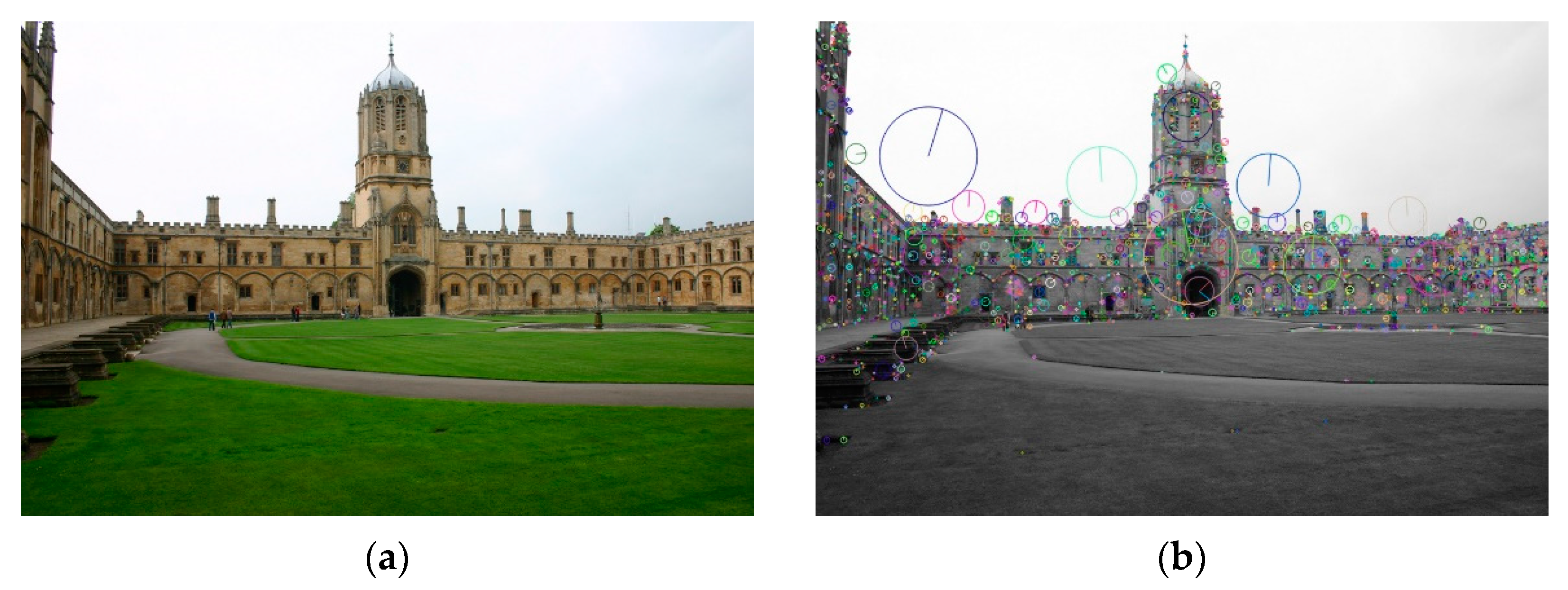
After assigning the scale, position, and direction information to each feature point, a feature descriptor needs to be defined for object matching. In this research, a 16 × 16 template-sized window is taken as the center of feature points and divided into 16 4 × 4 subblocks. The gradient size and histogram of the gradient direction in 8 directions including 0°, 45°, 90°, 135°, 180°, 225°, 270°, and 315° are calculated on each subblock [35]. Therefore, a 4×4 subblock can obtain a descriptor with 8 directions, and then 16 subblocks can obtain 128 direction descriptors, and the 1 × 128 dimensions vector is named as a feature descriptor vector. Figure 1 describes the key points through SIFT.

2.3. Accurate Matching of Feature Points Based on the IIR Algorithm

2.3.1. A Universal Framework for RANSAC

After roughly matching with SIFT, some missing matching pairs will inevitably occur. To eliminate the error caused by false matching, the RANSAC algorithm is a good and accurate matching algorithm [38]. However, low efficiency, slow speed, and easy degradation are three limitations of the classic RANSAC algorithm [39]. On this basis, many improved algorithms have flourished. Rahul et al. [11] presented a comprehensive overview and provided a universal framework called USAC for RANSAC algorithm, by analyzing and comparing various methods, which have been deeply explored over the years. For different modules, different algorithms that have been proved effective can be used.

2.3.2. The IIR Algorithm

In the improved RANSAC (I-RANSAC) algorithm [12], the fundamental purpose is to construct the optimal Homography matrix $\mathit{H}$, which refers to the invertible homogeneous transformations between two planes, plays a very important role in multi-view image. Then, the coordinate transformation can be shown as follows:

$$\left[\begin{array}{c}{x}_b\\ y_b\\ 1\end{array}\right]=\left[\begin{array}{ccc}{h}_0& h_1& h_2\\ h_3& h_4& h_5\\ h_6& h_7& 1\end{array}\right]\left[\begin{array}{c}{x}_a\\ y_a\\ 1\end{array}\right].$$

(11)

In Equation (11), $(x_a,y_a)$ and $(x_b,y_b)$ are respectively the image coordinates before and after the transformation.

$$\mathit{H}=\left[\begin{array}{ccc}{h}_0& h_1& h_2\\ h_3& h_4& h_5\\ h_6& h_7& 1\end{array}\right].$$

(12)

In Equation (12), h₀~h₇ are eight parameters in the Homography matrix $\mathit{H}$, which can be calculated by selecting 4 feature points, i.e., four-point algorithm [12,40], on each of the two images.

However, when the I-RANSAC algorithm shown in Ref. [12] is adopted to achieve image matching, if the number of image feature points obtained after SIFT processing is large and the degree of correlation between feature points is small, then the difficulty of acquiring the Homography matrix increases, which affects the matching accuracy and matching time of the image feature points. To meet the requirements of simultaneously improving the accuracy and speed, on the basis of RANSAC universal framework, this paper proposes IIR in the module of model generation to optimize the Homography matrix through a decision rule for the total number of interior points. The specific implementation process is given below.

Firstly, 4 pairs of feature points that are not on the same line are randomly selected after the rough matching with SIFT, and the distance among the matching points can be calculated, which is denoted as a set $d_H$. The purpose of selecting 4 pairs of non-collinear matching points is to solve the 8 parameters in the Homography matrix $\mathit{H}$ and obtain the unique Homography matrix $\mathit{H}$ [41].

Secondly, the ratio of the nearest distance $d_{\min }$ and sub-nearest distance $d_{\min 0}$ should be calculated according to the nearest-neighbor principle in $d_H$, and then the results will be divided into 4 groups from large to small.

Thirdly, the number of inner points $T_H$ for the 4 groups of matching pairs that are randomly selected in the group with the smallest ratio are calculated. If $T_H\ge 3$, then the selected matching pair is retained, and the remaining matching pairs are successively executed in the above process; otherwise, 4 groups of feature points are randomly selected again for the operation.

Finally, a comparison is made between the accumulated inner points $T_{Hall}$ and the pre-set threshold $T_{H0}$. If $T_{Hall}\ge T_{H0}$, then the total process finishes; otherwise, it is restarted.

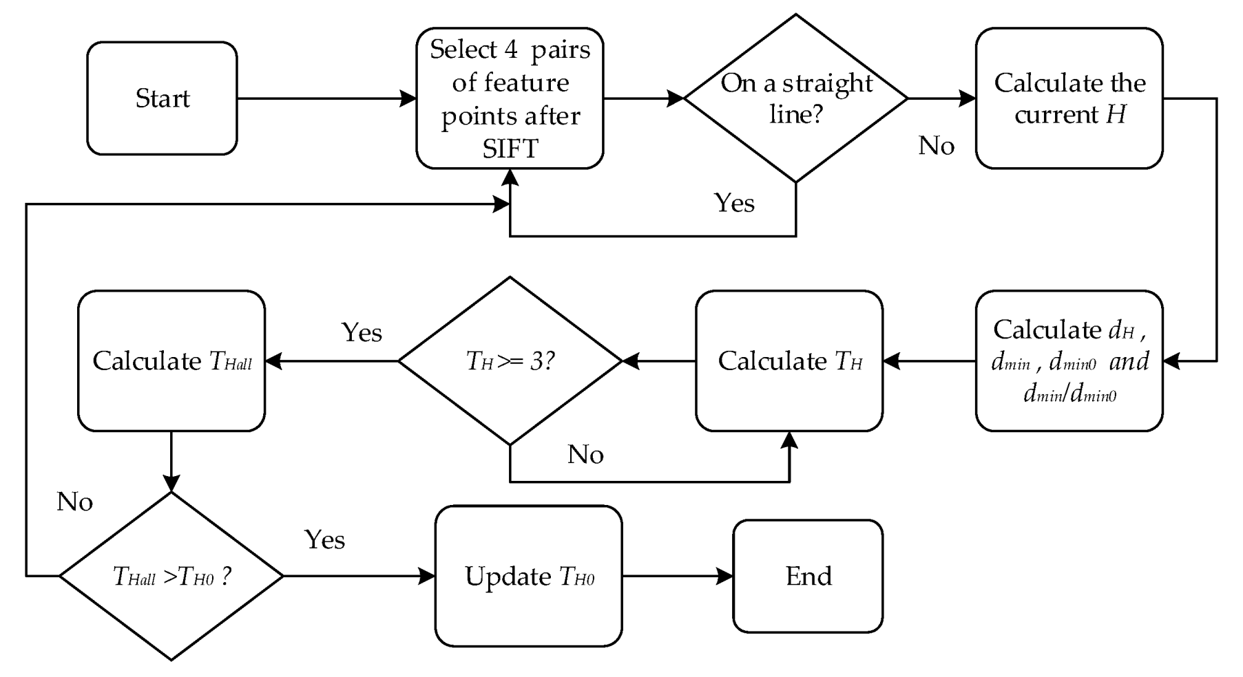
A flow chart for IIR is shown in Figure 2.

Depending on the aforementioned steps and flow chart, in IIR algorithm, the distance among the matching points can be calculated, while the ratios of the nearest distance $d_{\min }$ and sub-nearest distance $d_{\min 0}$ are divided into 4 groups from large to small, with the principle of nearest-neighbor. Thus, when selecting matching pairs from the smallest ratio group, it can ensure that the selected matching pairs are evenly distributed in the image, which can avoid selecting some isolated feature points. In addition, the judging condition $T_H\ge 3$ means that most of the feature points selected from the smallest ratio group have the same area attributes and model attributes. Therefore, the conditions that these feature points satisfied should remain unchanged. Finally, by comparison of the accumulated inner points $T_{Hall}$ and threshold $T_{H0}$, the current Homography matrix can be updated and optimized, which is likewise the purpose of IIR algorithm.

2.4. Image Fusion Method

After image registration, if the method of direct fusion is adopted, the fusion effect will be stiff and it is easy to produce an obvious image seam and then the fusion image will be blurred due to the simple addition of pixels. Therefore, the method of weighted smoothing is adopted in this paper for image fusion [42].

It is assumed that $F_1(x_1,y_1)$ and $F_2(x_2,y_2)$ are respectively the pixel values of the two images to be fused at the indexes of $(x_1,y_1)$ and $(x_2,y_2)$; $F_3(x_3,y_3)$ are the pixel values of the fusion image at the index of $(x_3,y_3)$; $w_{F_1}$ and $w_{F_2}$ are the weights of the two images to be fused, respectively. The fusion condition should be satisfied as follows.

$$F_3(x_3,y_3)=\left\{\begin{array}{l}{F}_1(x_1,y_1),(x_3,y_3)\in F_1\\ F_2(x_2,y_2),(x_3,y_3)\in F_2\\ w_{F_1}\times F_1(x_1,y_1)+w_{F_2}\times F_2(x_2,y_2),(x_3,y_3)\in F_1\cap F_2\end{array}\right.$$

(13)

In Equation (13), $w_{F_1}$ and $w_{F_2}$ are related to the width of the overlapping region of the two images, and $0<w_{F_1},w_{F_2}<1$, and $w_{F_1}+w_{F_2}=1$. In practice, $w_{F_1}$ should be slowly reduced from 1 to 0 and $w_{F_2}$ should be slowly increased from 0 to 1 in the overlapping region of the two images to achieve the smooth transition of the weight.

3. Results and Discussion

In this study, image mosaic refers to combining two original images with overlapping regions into one image, which is completed through three steps including image enhancement, image registration, and image fusion. The two original images are respectively defined as the reference image and the be-registered image (the image to be registered). The former can be regarded as a standard reference image without any change, and the latter will be mapped to the former via the spatial transformation with dynamic change. The image processing platform was unified as one laptop, and the detailed information of which was as follows: Windows 10 system, Intel(R) Core(TM) i5-7200u CPU @2.50 GHz 2.71 GHz, and 8 GB of memory.

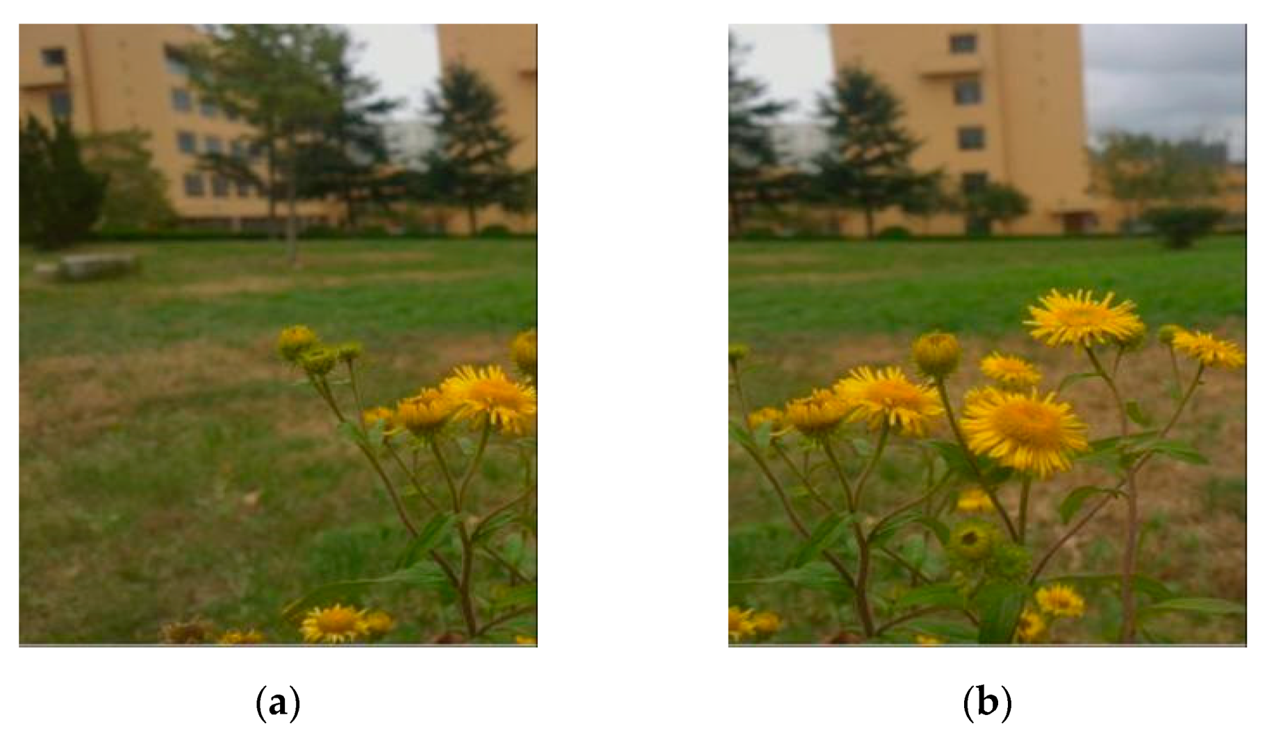
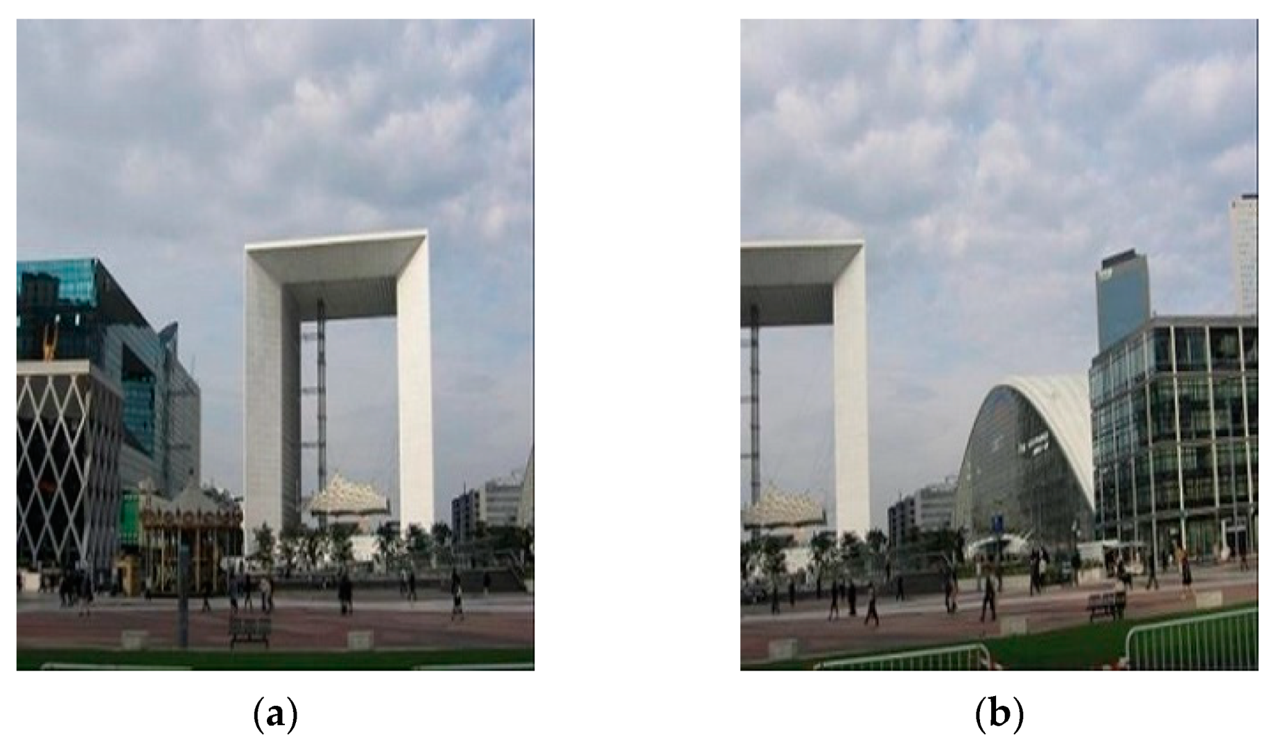
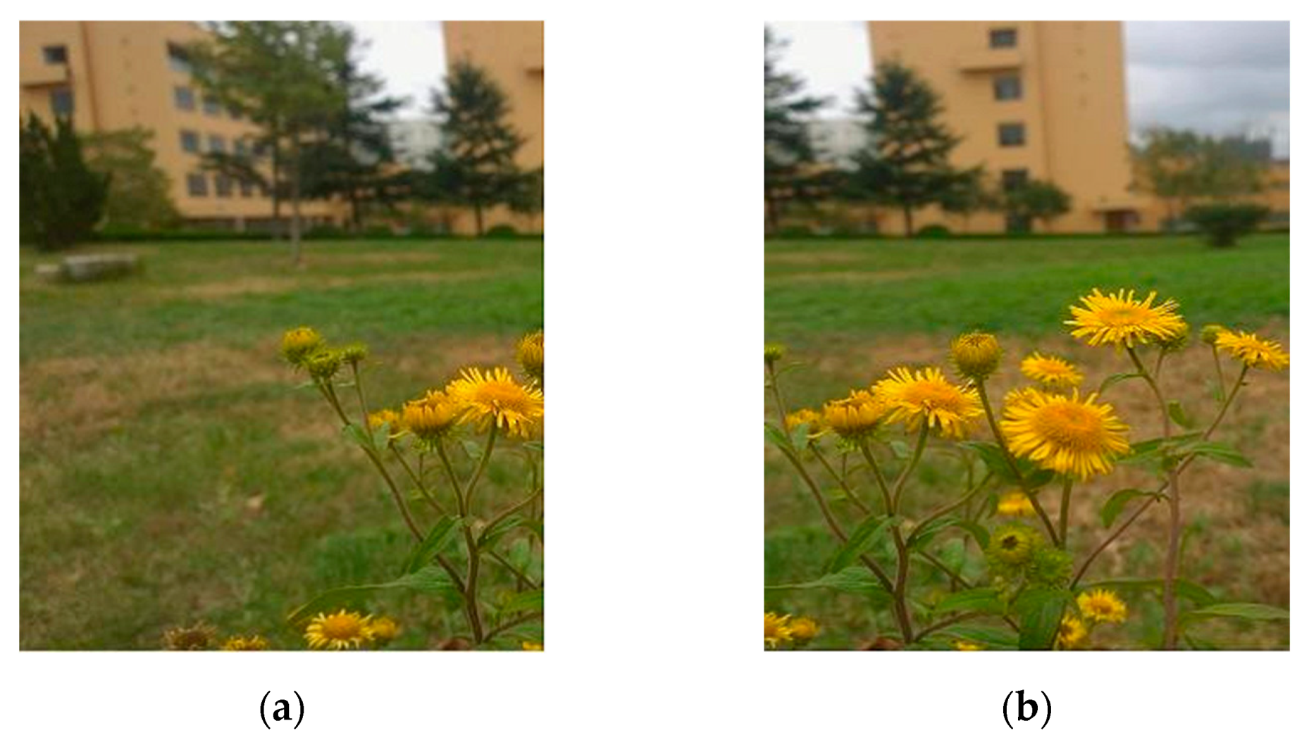
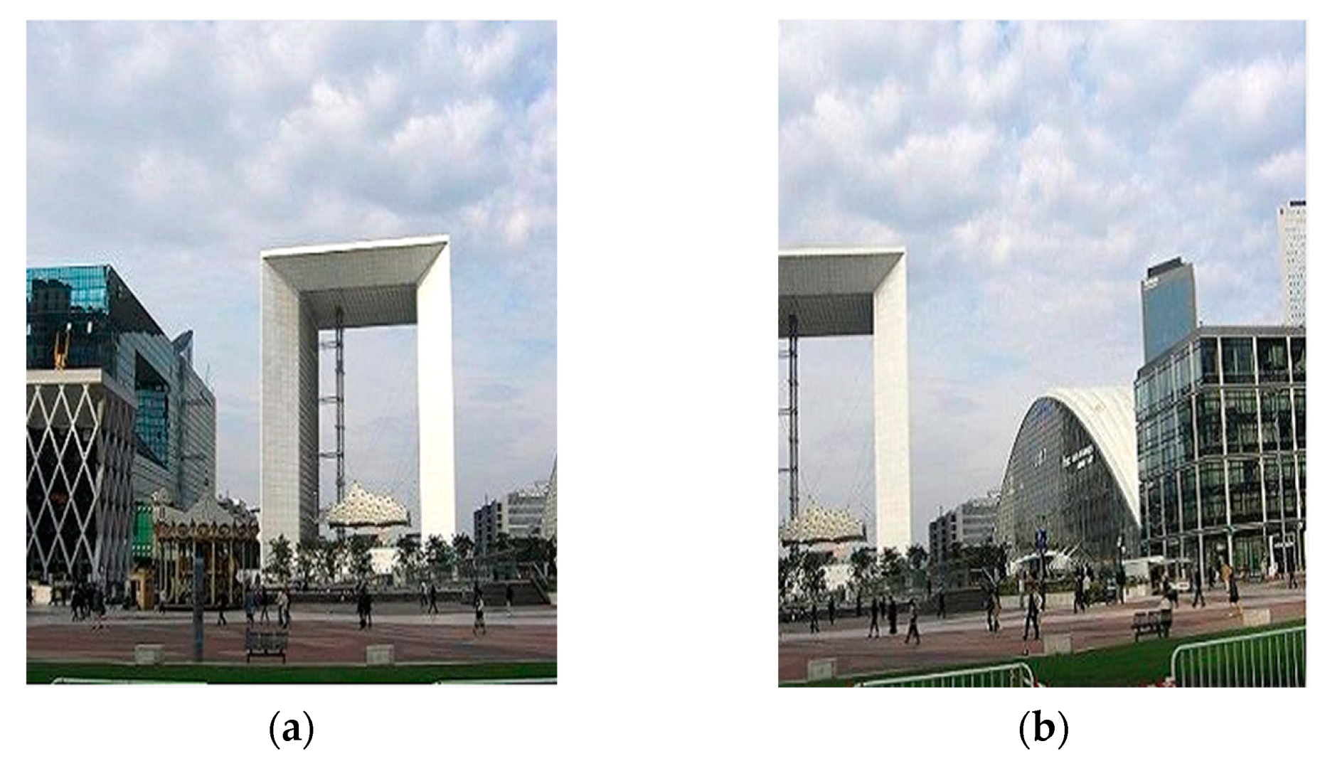
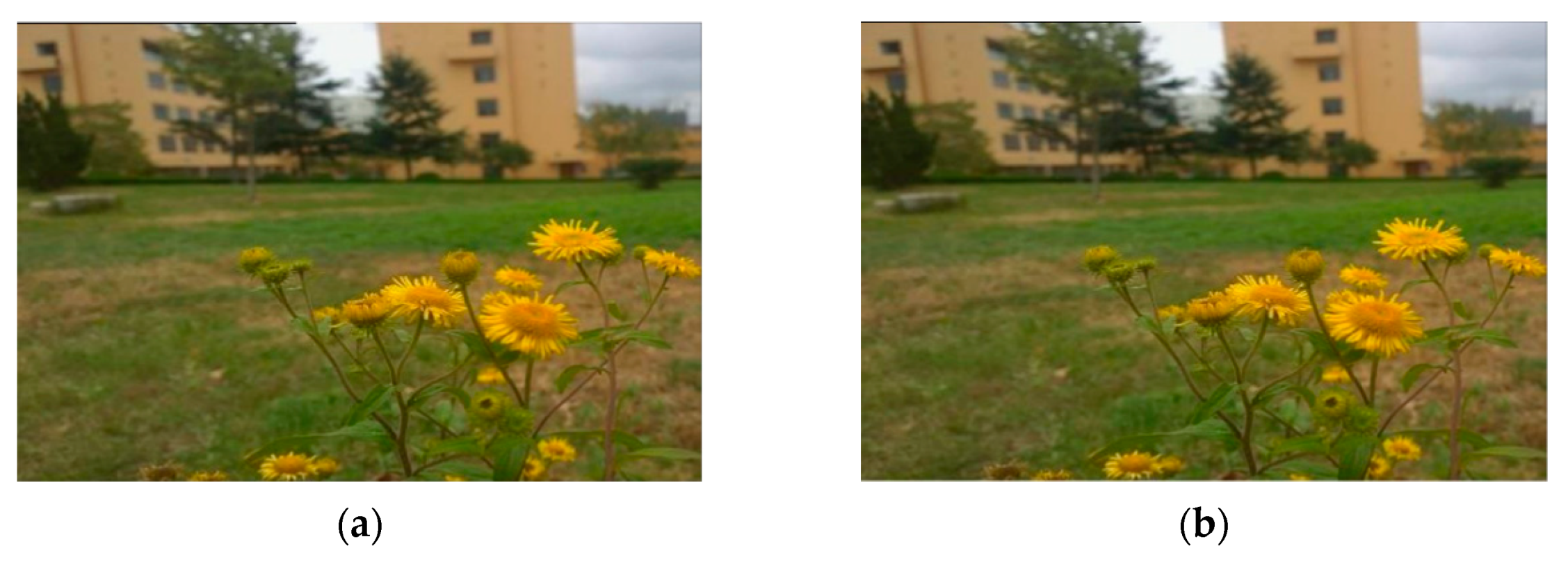
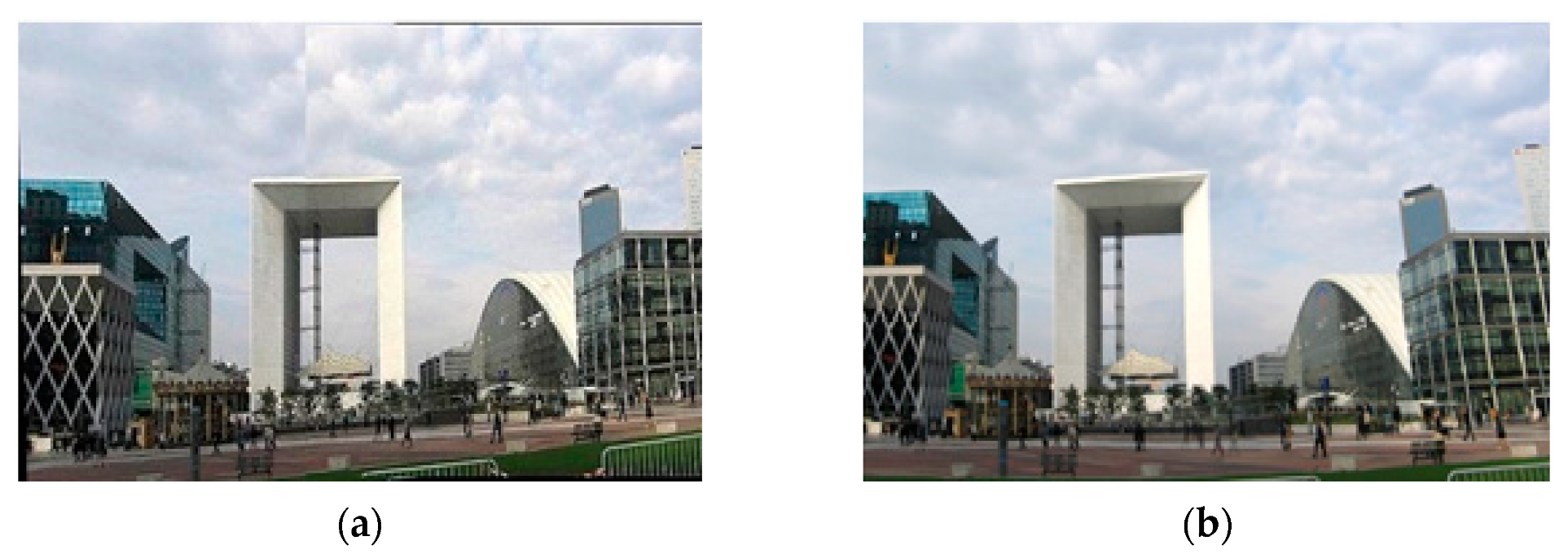
Firstly, two-group images (four images) with low contrast and low definition were randomly selected as experimental objects from the Oxford Buildings Dataset, as shown in Figure 3 and Figure 4. The two-group images are named T1 and T2; and the original images of each group included a reference image and a be-registered image that corresponded to Sub-figure (a) and Sub-figure (b), respectively.

After mixed method and sigma filtering, Figure 5 and Figure 6 are the enhanced results of the two-group images. To evaluate the enhancement effect quantitatively, three indexes, including the mean square error $\alpha$, the peak signal-to-noise ratio $\beta$, and one-dimensional image entropy $\gamma$, were used to evaluate the image quality before and after enhancement.

Table 1. Three image quality indexes of T1 and T2.

Group	$\mathit{\alpha }$		$\mathit{\beta }$		$\mathit{\gamma }$
	Reference	Be-Registered	Reference	Be-Registered	Reference	Be-Registered
T1	8.42	9.13	49.87	49.28	0.03	0.02
T2	7.48	7.61	48.96	48.43	0.12	0.15
Mean	7.95	8.37	49.42	48.86	0.08	0.09

lists the specific information of the three indexes.

The improvement of the image contrast and definition can be visually seen in Figure 5 and Figure 6. Through a quantitative analysis of the data in Table 1, the average mean square error for the reference image and be-registered image were 7.95 and 8.37, respectively; the average peak signal-to-noise ratio for the reference image and be-registered image were 49.42 and 48.86, respectively; and the average one-dimensional image entropy for the reference image and be-registered image were 0.08 and 0.09, respectively. Therefore, the three indexes all meet the conditions of image non-distortion that the mean square error was smaller, the peak signal-to-noise ratio was larger, and the difference of one-dimensional entropy was also smaller. Thus, there was no artificial distortion between the enhanced images and the original images, and subsequent processes of the image registration and image fusion can be carried out.

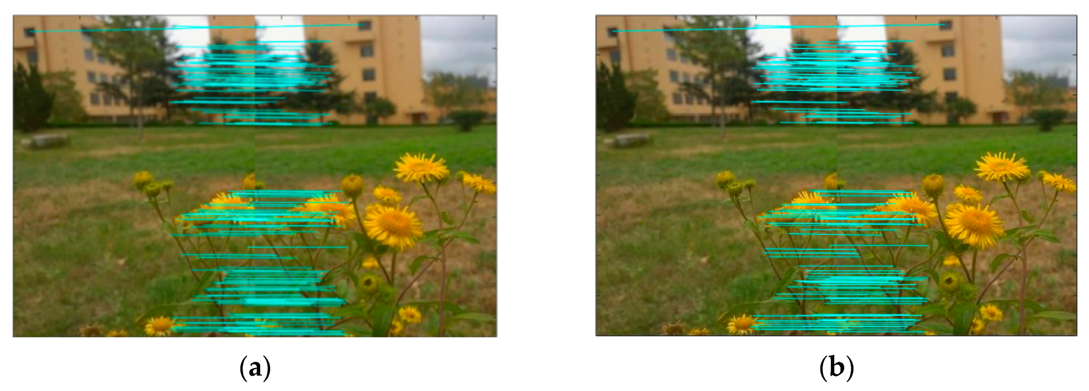
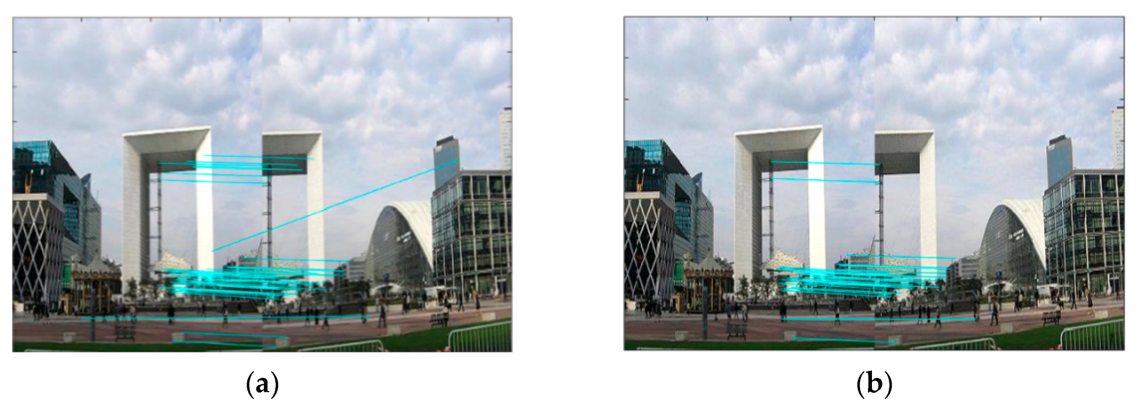
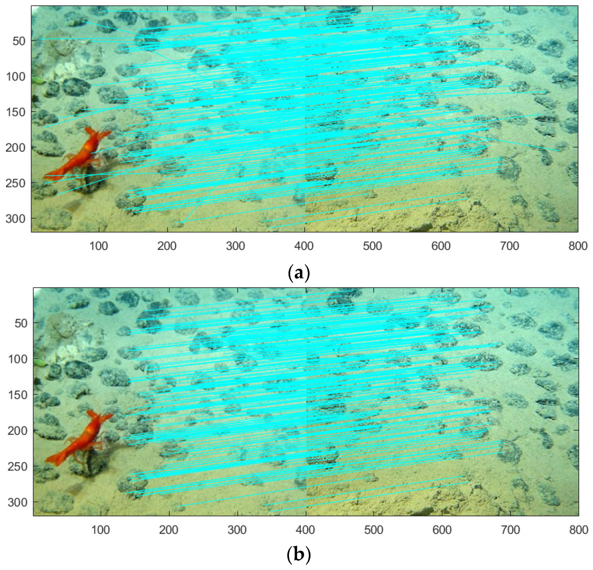
To prove that the proposed algorithm in this paper can effectively eliminate many mismatching points, Figure 7 and Figure 8 respectively show the image registration effect of two-group images processed by the I-RANSAC algorithm [12] and the IIR algorithm.

Compared to the I-RANSAC algorithm, in Figure 7 and Figure 8, the number of lines for matching points in the registration images by the IIR algorithm was greatly reduced, effectively avoiding some mismatching points. To quantitatively prove that the IIR algorithm can simultaneously improve the accuracy and speed in the process of image registration,

Table 2. A comparison of feature point information between two algorithms.

Algorithm	Group	Feature Point		Match Pair
		Reference	Be-Registered	Rough	Uniformly
I-RANSAC [15]	T1	541	856	213	190
	T2	1069	1087	124	109
IIR	T1	478	671	197	180
	T2	716	783	98	91

shows the specific information of feature points for the two-group images in image registration, and

Table 3. A comparison of the matching accuracy and matching time between different algorithms.

Features	Group	ORB [6]	FAST [4]	SURF [5]	I-RANSA [12]	IIR
Matching accuracy	T1	87.76	84.71	87.12	89.20	91.37
	T2	86.33	84.78	86.42	87.90	92.86
	Mean	87.04	84.74	86.77	88.55	92.12
Matching time	T1	2.58	2.17	2.35	2.63	2.43
	T2	2.89	2.53	2.78	2.94	2.88
	Mean	2.74	2.35	2.57	2.79	2.67

shows a comparison of the matching accuracy and matching time among five algorithms, i.e., ORB, FAST, SURF, I-RANSAC, and IIR.

Compared with the I-RANSAC algorithm, the IIR algorithm reduced the number of feature points and the number of consistent matching pairs, as shown in Table 2. The reason for this is that the improved algorithm is more rigorous in the selection of feature points and more accurate in the solution of the Homography matrix, which effectively eliminates the mismatching pairs. Moreover, accuracy and rapidity are two important indexes for image registration, which will be displayed as matching accuracy and matching time. According to Table 3, when compared with the I-RANSAC algorithm alone, the IIR algorithm can greatly improve the matching accuracy and matching time. Regarding the average matching accuracy and average matching time of the two-group images, the IIR algorithm improved the average matching accuracy by 3.54% and reduced the average matching time by 4.30%. When compared with the existing four algorithms of ORB, FAST, SURF, and I-RANSAC, the IIR algorithm was close to the four existing algorithms in matching time but it significantly improved the matching accuracy. The average matching accuracy was 92.12%, which was the best among the five algorithms.

Considering the randomness of the two groups of experimental images randomly selected, the experimental results may be unconvincing. Therefore, this paper conducts multiple groups of experiments to verify the effectiveness of the IIR algorithm by obtaining the mean ($M$) and standard deviation ($SD$).

Table 4. The information of matching accuracy with different groups of images.

Features	Group	ORB [6]	FAST [4]	SURF [5]	I-RANSAC [12]	IIR
		$\mathit{M}\pm \mathit{S}\mathit{D}$	$\mathit{M}\pm \mathit{S}\mathit{D}$	$\mathit{M}\pm \mathit{S}\mathit{D}$	$\mathit{M}\pm \mathit{S}\mathit{D}$	$\mathit{M}\pm \mathit{S}\mathit{D}$
Matching	5	87.13 ± 1.74	85.42 ± 2.52	86.96 ± 1.61	88.78 ± 1.51	89.34 ± 1.37
	10	88.34 ± 1.81	88.10 ± 2.04	88.27 ± 1.75	89.75 ± 1.28	91.26 ± 1.04
Accuracy	15	87.92 ± 1.56	87.68 ± 1.63	87.71 ± 1.38	88.96 ± 1.34	91.54 ± 1.16
	20	88.12 ± 1.18	87.83 ± 1.34	88.04 ± 0.96	89.41 ± 0.92	92.17 ± 0.87

shows the specific matching accurate information of the experimental images of different groups.

As shown in Table 4, with the increases of the number of groups, in IIR algorithm, the average of matching accuracy takes the first place, while at the same time, the standard deviation of matching accuracy is the smallest, among the five algorithms. So, it is obvious that the IIR algorithm is effective and stable in image registration.

To further prove that the IIR algorithm proposed in this paper can also partly improve the image fusion effect, Figure 9 and Figure 10 show the fusion effect of two-group images by the method of weighted smoothing after image registration through the I-RANSAC algorithm [12] and IIR algorithm.

As shown in Figure 9 and Figure 10, the same method of weighted smoothing was adopted to image fusion, but the final results were different. Compared with the I-RANSAC algorithm, the image fusion effect by the IIR algorithm is better because image seams disappear in the fusion images. The reason for this is that the IIR algorithm can eliminate more mismatching points in image registration, which improves the percentage of accurate matching pairs. Therefore, the fusion effect has also been improved. According to the above experimental results, the following conclusion can be drawn: the proposed IIR algorithm can simultaneously improve the matching accuracy and matching time.

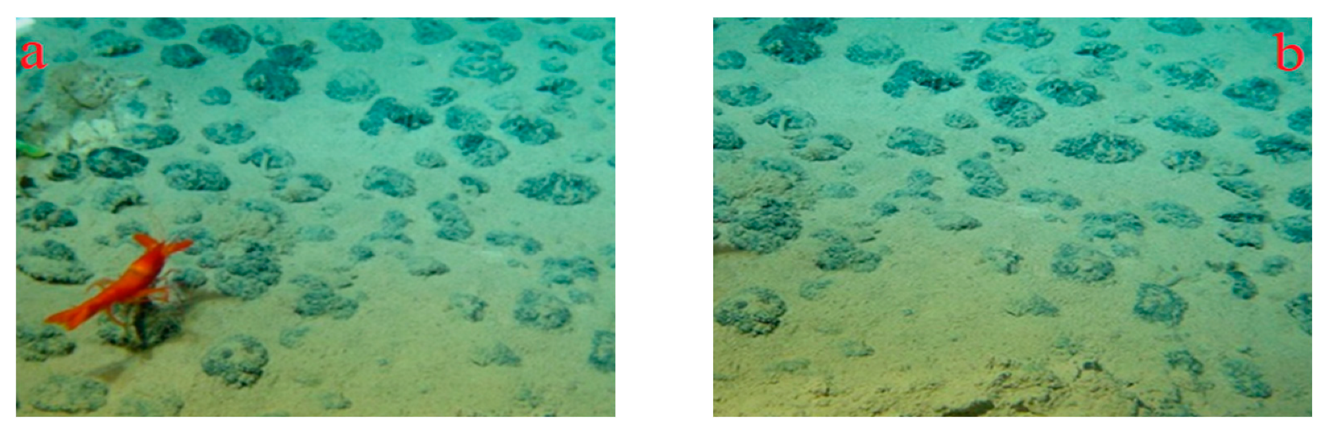
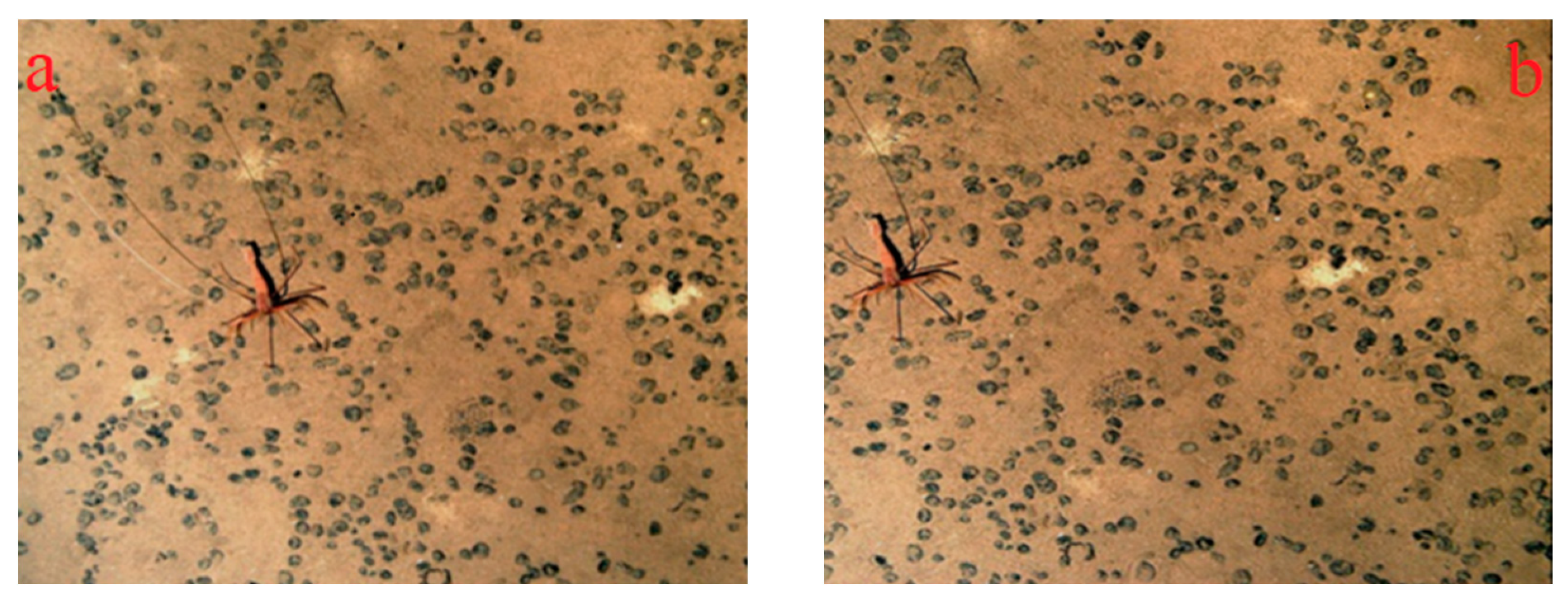
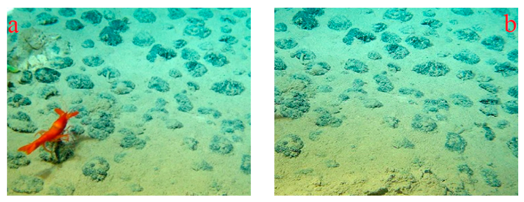
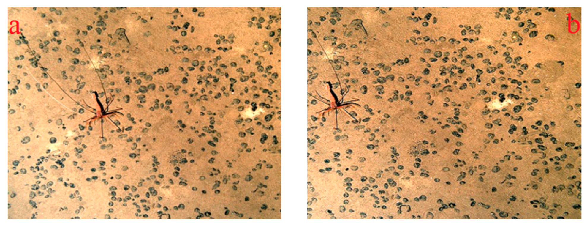
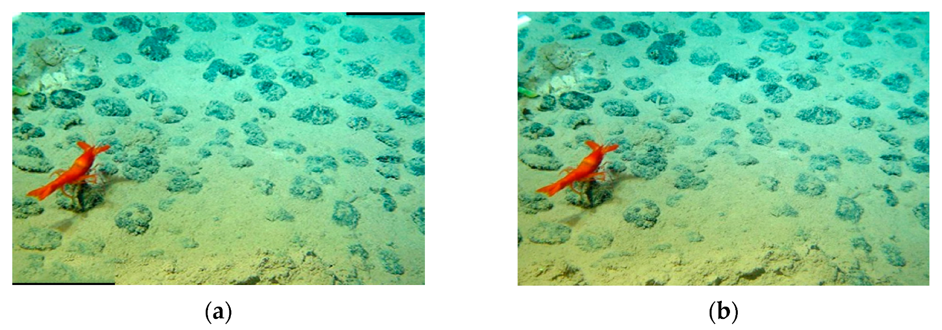
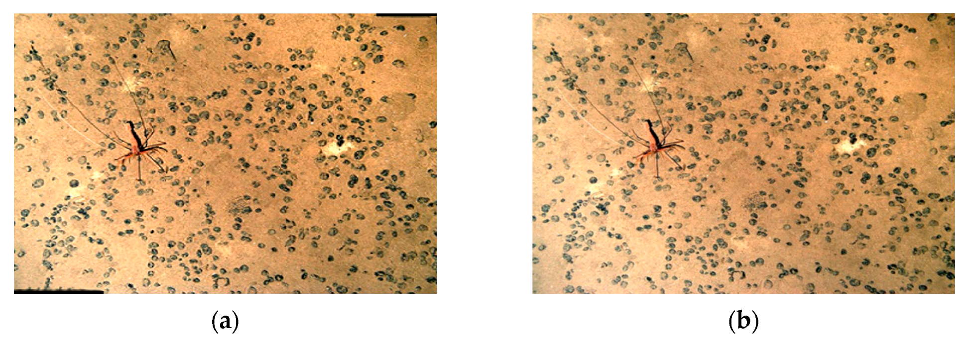
Due to the sharp increase of the research cruises, together with the large amounts of images and video recordings for underwater topography, it is a great demand for image mosaic and processing. We have demonstrated the effectiveness of the IIR algorithm in the Oxford Buildings Dataset and then applied it in underwater scenarios. The proposed algorithm has been used to study underwater image mosaic. Two-group images (four images) with low contrast and low definition were randomly selected as experimental objects from the image dataset of manganese nodules, as shown in Figure 11 and Figure 12. Specifically, four images were segmented from the two original images. The purpose of that is to obtain the experimental images with similar sizes and attributes and make the appropriate overlap area between the reference image and be-registered image. Then, two-group images were named T3 and T4, respectively; and the original images of each group similarly included the reference image and be-registered image, which corresponded to Sub-figure (a) and Sub-figure (b).

Similar to the process of T1 and T2, Figure 13 and Figure 14 show the enhancement effect of the two-group underwater images. Also, the information of three image quality evaluation indexes corresponding to each group before and after the process of image enhancement is given in

Table 5. Three image quality indexes of T3 and T4.

Group	$\mathit{\alpha }$		$\mathit{\beta }$		$\mathit{\gamma }$
	Reference	Be-Registered	Reference	Be-Registered	Reference	Be-Registered
T3	0.49	0.37	55.23	55.44	0.01	0.04
T4	0.62	0.57	57.43	57.97	0.12	0.09
Mean	0.56	0.47	56.33	56.71	0.07	0.07

.

Compared with Figure 11 and Figure 12, the image contrast and definition in Figure 13 and Figure 14 are significantly improved, which can be intuitively sensed by the naked eye. A quantitative analysis of the data in Table 5 shows that the average mean square error for the reference image and the be-registered image were 0.56 and 0.47, respectively; the average peak signal to noise ratio for the reference image and be-registered image were 56.33 and 56.71, respectively; and the average one-dimensional image entropy for the reference image and the be-registered image both were 0.07. Therefore, the three indexes better meet the conditions of image non-distortion that the mean square error was smaller, the peak signal-to-noise ratio was larger, and the difference of one-dimensional entropy was smaller as well. Thus, the subsequent processes of image registration and image fusion can also be carried out.

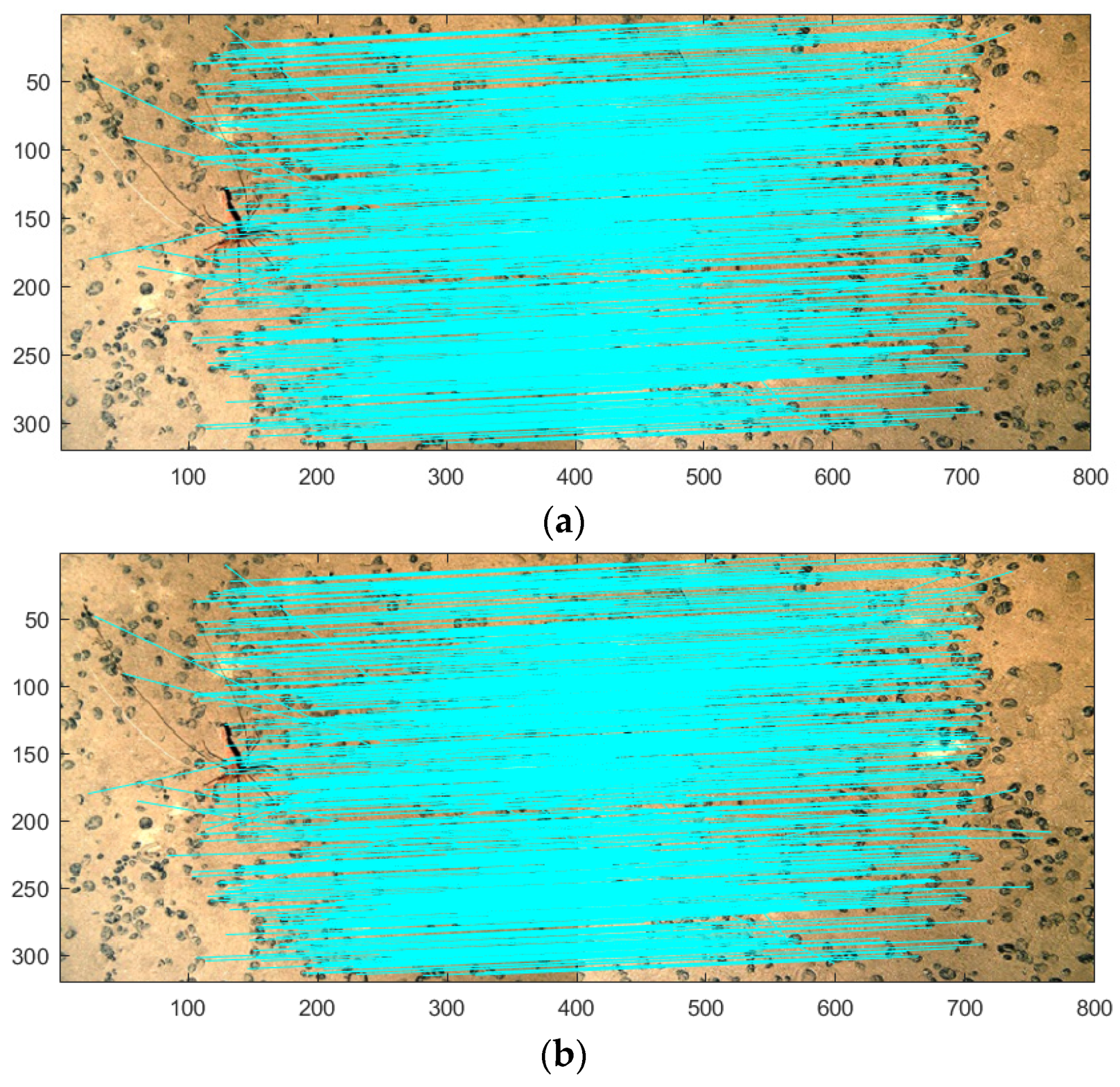
To prove that the proposed algorithm in this paper can also effectively eliminate many mismatching points on underwater images, Figure 15 and Figure 16 respectively show the image registration effect of two-group images processed by the I-RANSAC algorithm [12] and the IIR algorithm.

As shown in Figure 15 and Figure 16, compared with the I-RANSAC algorithm, the number of lines for matching points in the registration images by the IIR algorithm was reduced, effectively avoiding some mismatching points. To quantitatively prove that the IIR algorithm can simultaneously improve the accuracy and speed in the process of image registration,

Table 6. A comparison of feature point information between two algorithms.

Algorithm	Group	Feature Point		Match Pair
		Reference	Be-Registered	Rough	Uniformly
I-RANSAC [15]	T3	2103	2269	740	690
	T4	2344	2648	816	735
IIR	T3	1686	1761	623	586
	T4	1851	2096	676	628

shows the specific information of the feature points for the two-group images in image registration.

Table 7. A comparison of matching accuracy and matching time between different algorithms.

Features	Group	ORB [6]	FAST [4]	SURF [5]	I-RANSAC [12]	IIR
Matching accuracy	T3	90.10	87.46	91.13	93.24	94.06
	T4	87.62	85.37	88.36	90.07	92.90
	Mean	88.86	86.42	89.75	91.66	93.48
Matching time	T3	2.39	2.21	2.33	2.51	2.42
	T4	2.46	2.28	2.41	2.61	2.49
	Mean	2.43	2.25	2.37	2.56	2.46

shows a comparison of the matching accuracy and matching time among the ORB, FAST, SURF, I-RANSAC, and IIR algorithms.

Compared with the I-RANSAC algorithm, the IIR algorithm reduced the number of feature points and the number of consistent matching pairs, as shown in Table 6. The reason for this is that the improved algorithm is more rigorous in the selection of feature points and more accurate in the solution of the homology matrix, which effectively eliminates the mismatching pairs. Moreover, according to Table 7, when compared to the I-RANSAC algorithm alone, the IIR algorithm can improve the matching accuracy and matching time. Regarding the average matching accuracy and average matching time of the two-group images, the IIR algorithm improved the average matching accuracy by 3.54% and reduced the average matching time by 4.30%. Compared to the existing four algorithms (ORB, FAST, SURF, and I-RANSAC), the IIR algorithm is close to the four existing algorithms in matching time but significantly improved the matching accuracy. The average matching accuracy was 92.12%, which was the best among the five algorithms.

To further prove that the IIR algorithm can also partly improve the image fusion effect, Figure 17 and Figure 18 show the fusion effect of two-group images by the method of weighted smoothing after image registration through the I-RANSAC algorithm [12] and IIR algorithm.

The same method of weighted smoothing was adopted for image fusion, but the final results are different, as shown in Figure 17 and Figure 18. Compared to the I-RANSAC algorithm, the image fusion effect by the IIR algorithm was better because the image seams disappeared in the fusion images. The reason for this is that the IIR algorithm can eliminate more mismatching points in image registration, which improves the percentage of accurate matching pairs. Therefore, the fusion effect is also improved. Therefore, the algorithm in this paper also has a good application in underwater image mosaic, which cannot only improve the accuracy and rapidity but also improve the image mosaic quality.

4. Conclusions

The problems of image registration and image fusion are studied in this paper. Firstly, mixed method and sigma filtering are used to enhance the images with low contrast and low definition. Then, IIR is proposed for image registration based on USAC. Finally, the method of weighted smoothing is used for image fusion. We tested the IIR algorithm via the Oxford Buildings Dataset to verify the effectiveness. Then, the algorithm was applied in an underwater environment. Compared with ORB, FAST, SURF, and I-RANSAC algorithms, the quantitative analysis results show the IIR algorithm can reduce the number of feature points and that of consistent matching points, and improve the fast index and accurate index. Furthermore, the algorithm in this paper avoids the appearance of image seams in the image quality, thus improving the image fusion effect.

References

- Hines, D. Immediate and delayed recognition of sequentially presented random shapes. J. Exp. Psychol. Hum. Learn. Mem. 1975, 1, 634–639. [Google Scholar] [CrossRef]
- Harris, C.; Stephens, M. A Combined Corner and Edge Detector. In Proceedings of the 4th Alvey Vision Conference, Alvey, UK, 31 August–2 September 1988; pp. 147–151. [Google Scholar]
- Lowe, D.G. Distinctive image features from scale-invariant keypoints. Int. J. Comput. Vis. 2004, 60, 91–110. [Google Scholar] [CrossRef]
- Rosten, E.; Tom, D. Machine learning for high-speed corner detection. In Proceedings of the 7th European Conference on Computer Vision, Berlin, Germany, 7–13 May 2006; Springer: Berlin, Germany, 2006; pp. 430–443. [Google Scholar]
- Bay, H.; Ess, A.; Tuytelaars, T. Speeded-up robust features (SURF). Comput. Vis. Image Underst. 2008, 110, 346–359. [Google Scholar] [CrossRef]
- Michael, C.; Vincent, L.; Pascal, F. Brief: Binary robust independent elementary features. In Proceedings of the 11th European Conference on Computer Vision, Hersonissos, Greece, 5–11 September 2010; Springer: Hersonissos, Greece, 2010; pp. 778–792. [Google Scholar]
- Ghosh, D.; Kaabouch, N. A survey on image mosaicing techniques. J. Vis. Commun. Image Represent. 2016, 34, 1–11. [Google Scholar] [CrossRef]
- Liu, J.; Fu, W.P.; Wang, W. Image matching based on improved SIFT algorithm. Chin. J. Sci. Instrum. 2017, 35, 1107–1112. [Google Scholar]
- Zhu, Z.W.; Shen, Z.F.; Luo, J.C. Parallel remote sensing image registration based on improved SIFT point feature. J. Remote Sens. 2011, 15, 1024–1039. [Google Scholar]
- Yi, N.J.; Wu, D.W.; Qi, J.Y. A method to extract high robust keypoints based on improved SIFT. Chin. J. Aeronaut. 2012, 33, 2313–2321. [Google Scholar]
- Raguram, R.; Chum, O.; Pollefeys, M.; Matas, J.; Frahm, J.-M. USAC: A universal framework for random sample consensus. IEEE Trans. Pattern Anal. Mach. Intell. 2013, 35, 2022–2038. [Google Scholar] [CrossRef]
- Shi, G.J.; Xu, X.Y.; Dai, Y.P. SIFT feature point matching based on improved RANSAC algorithm. In Proceedings of the Fifth International Conference on Intelligent Human-Machine Systems and Cybernetics, Hangzhou, China, 26–27 August 2013; IEEE Press: Hangzhou, China, 2013; pp. 474–477. [Google Scholar]
- Li, B.; Ming, D.L.; Yan, W.W. Image matching based on two-column histogram hashing and improved RANSAC. IEEE Geosci. Remote Sens. Lett. 2014, 11, 1433–1437. [Google Scholar]
- Zhao, M.F.; Chen, H.J.; Song, T.; Deng, S.X. Research on image matching based on improved RANSAC-SIFT algorithm. Laser J. 2017, 7, 114–118. [Google Scholar]
- Eduardo, M.; Sonia, M.; Carlos, S. Distributed robust consensus using RANSAC and dynamic opinions. IEEE Trans. Control Syst. Technol. 2015, 23, 150–163. [Google Scholar]
- Gao, X.; Luo, J.Z.; Li, K.Q.; Xie, Z.X. Hierarchical RANSAC-based rotation averaging. IEEE Signal Process. Lett. 2020, 27, 1874–1878. [Google Scholar] [CrossRef]
- Lati, A.; Belhocine, M.; Achour, N. Robust aerial image mosaicing algorithm based on fuzzy outliers rejection. Evol. Syst. 2020, 11, 717–729. [Google Scholar] [CrossRef]
- Meher, B.; Agrawal, S.; Panda, R.; Abraham, A. A survey on region based image fusion methods. Inf. Fusion 2019, 48, 119–132. [Google Scholar] [CrossRef]
- Chen, M.M.; Rui, N.; Bo, H.; Qiu, S.Q.; Yan, T.H. Underwater image stitching based on SIFT and wavelet fusion. In Proceedings of the Oceans 2015, Genova, Italy, 18–21 May 2015; IEEE Press: Genova, Italy, 2015; pp. 12–17. [Google Scholar]
- Xie, Y.L.; Li, X.F.; Lv, J.W. Real-time underwater image registration based on SURF algorithm. J. Comput. Aided Des. Comput. Graph. 2010, 22, 2215–2220. [Google Scholar]
- Rahul, R.; Shishir, R.; Karen, P.; Sos, A. Adaptive alpha-trimmed correlation based underwater image stitching. In Proceedings of the IEEE International Symposium on Technologies for Homeland Security (HST), Waltham, MA, USA, 25–26 April 2017; IEEE Press: Waltham, MA, USA, 2017; pp. 32–39. [Google Scholar]
- Li, H.L.; Huang, Y.Q.; Zhang, Z.J. An improved faster R-CNN for same object retrieval. IEEE Access 2017, 5, 13665–13676. [Google Scholar] [CrossRef]
- Kovalevsky, V. Modern Algorithms for Image Processing; Apress: Berkeley, CA, USA, 2019. [Google Scholar] [CrossRef]
- Dong, L.L.; Ding, C.; Xu, W.H. Two improved methods based on histogram equalization for image enhancement. Chin. J. Electron. 2018, 46, 65–73. [Google Scholar]
- Majid, Z.; Ali, P.; Hassan, H. Image contrast enhancement using triple clipped dynamic histogram equalisation based on standard deviation. IET Image Process. 2019, 13, 1081–1089. [Google Scholar]
- Stimper, V.; Bauer, S.; Ernstorfer, R.; Schölkopf, B.; Xian, R.P. Multidimensional contrast limited adaptive histogram equalization. IEEE Access 2019, 7, 35–51. [Google Scholar]
- Gao, F.; Wang, K.; Yang, Z.; Wang, Y.; Zhang, Q. Underwater image enhancement based on local contrast correction and multi-scale fusion. J. Mar. Sci. Eng. 2021, 9, 225. [Google Scholar] [CrossRef]
- Yanling, H.; Lihua, H.; Zhonghua, H.; Shouqi, C.; Yun, Z.; Jing, W. Deep supervised residual dense network for underwater image enhancement. Sensors 2021, 21, 3289. [Google Scholar]
- Zhang, H.; Lei, Z.H.; Ding, X.H. Improved method of median filter. China J. Image Graph. 2004, 9, 408–411. [Google Scholar]
- Deniz, L.G.; Buemi, M.E.; Julio, J.B.; Mejail, M. A new image quality index for objectively evaluating despeckling filtering in SAR Images. IEEE J. Sel. Top. Appl. Earth Obs. Remote Sens. 2016, 9, 1297–1307. [Google Scholar]
- Jiang, G.Y.; Huang, D.J.; Wang, X. Overview on image quality assessment methods. J. Electron. Inf. Technol. 2010, 32, 219–226. [Google Scholar] [CrossRef]
- Amir, K.; Orly, Y.P. Quaternion structural similarity: A new quality index for color images. IEEE Trans. Image Process. 2012, 21, 1526–1536. [Google Scholar]
- Kede, M.; Hojatollah, Y.; Zeng, K.; Zhou, W. High dynamic range image compression by optimizing tone mapped image quality index. IEEE Trans. Image Process. 2015, 24, 3086–3097. [Google Scholar] [CrossRef]
- Dellinger, F.; Delon, J.; Gousseau, Y.; Michel, J.; Tupin, F. SAR-SIFT: A SIFT-Like algorithm for SAR Images. IEEE Trans. Geosci. Remote Sens. 2015, 53, 453–466. [Google Scholar] [CrossRef] [Green Version]
- Li, Y.M.; Zhou, J.T.; Cheng, A.; Liu, X.M.; Tang, Y.Y. SIFT keypoint removal and injection via convex relaxation. IEEE Trans. Inf. Forensics Secur. 2016, 11, 1722–1735. [Google Scholar] [CrossRef]
- Fu, W.P.; Qing, C.; Liu, J. Matching and location of image object based on SIFT algorithm. Chin. J. Sci. Instrum. 2011, 6, 165–171. [Google Scholar]
- Philbin, J.; Chum, O.; Isard, M.; Sivic, J.; Zisserman, A. In object retrieval with large vocabularies and fast spatial matching. In Proceedings of the 2007 IEEE Conference on Computer Vision and Pattern Recognition, Minneapolis, MN, USA, 17–22 June 2007; pp. 1–8. [Google Scholar]
- Fischler, M.A.; Bolles, R.C. Random sample consensus: A paradigm for model fitting with applications to image analysis and automated cartography. Commun. ACM 2015, 24, 381–395. [Google Scholar] [CrossRef]
- Schnabel, R.; Wahl, R.; Klein, R. Efficient RANSAC for point-cloud shape detection. Comput. Graph. Forum 2010, 26, 214–226. [Google Scholar] [CrossRef]
- Chen, C.S.; Cheng, J.; Huang, Y.P. RANSAC-based DARCES: A new approach to fast automatic registration of partially overlapping range images. IEEE Trans. Pattern Anal. Mach. Intell. 1999, 21, 1229–1234. [Google Scholar] [CrossRef] [Green Version]
- Ascencio, C. Estimation of the Homography matrix to image stitching. In Applications of Hybrid Metaheuristic Algorithms for Image Processing; Oliva, D., Hinojosa, S., Eds.; Springer International Publishing: Cham, Switzerland, 2020; pp. 205–230. [Google Scholar]
- Chen, H.Y.; Ren, Y.F.; Cao, J.Q.; Liu, W.P.; Liu, K. Multi-exposure fusion for welding region based on multi-scale transform and hybrid weight. Int. J. Adv. Manuf. Technol. 2019, 101, 105–117. [Google Scholar] [CrossRef]
- Weaver, P.P.E.; Billett, D. Environmental impacts of nodule, crust and sulphide mining: An overview. In Environmental Issues of Deep-Sea Mining: Impacts, Consequences and Policy Perspectives; Sharma, R., Ed.; Springer International Publishing: Cham, Switzerland, 2019; pp. 27–62. [Google Scholar]
Figure 1.
SIFT key point detection. (a) is the input image [37]. and (b) is the key point description image, which is represented by a small circle at the function position, and the direction of the feature points will be displayed inside the circle. (Source: The Oxford Buildings Dataset).
Figure 2.
IIR algorithm flow chart. The goal of IIR algorithm is to obtain the optimal Homography matrix, and then to realize the accurate coordinate space transformation; that is, to delete and select the correct feature matching pairs.
Figure 3.
The original images for T1: (a) Reference image; (b) Be-registered image. Reference image is regarded as a standard reference image without any changes, and Be-registered image is mapped to the former through dynamic spatial transformation.
Figure 4.
The original images for T2: (a) Reference image; (b) Be-registered image.
Figure 5.
The improved images for T1: (a) Reference image; (b) Be-registered image.
Figure 6.
The improved images for T2: (a) Reference image; (b) Be-registered image.
Figure 7.
The registered images for T1: (a) I-RANSAC; (b) IIR. The blue line indicates the corresponding matching points of the two pictures. The registration accuracy of T1 (a) is 89.20%, and that of T1 (b) is 91.37%, as shown in Table 3.
Figure 8.
The registered images for T2: (a) I-RANSAC; (b) IIR. In complex scenarios, I-RANSAC mismatches, as shown in T2 (a), and IIR eliminates mismatches, as shown in T2 (b).
Figure 9.
The fusion images for T1: (a) I-RANSAC; (b) IIR. The image fusions of T1 (a) and T1 (b) in a simple scene have achieved good results.
Figure 10.
The fusion images for T2: (a) I-RANSAC; (b) IIR for T2 (a), I-RANSAC registration was used, and the fused images showed stitching traces; for T2 (b), IIR registration was used, and the fused images showed no stitching traces.
Figure 11.
The original images for T3: (a) Reference image [21]; (b) Be-registered image.
Figure 12.
The original images for T4: (a) Reference image [43]; (b) Be-registered image.
Figure 13.
The improved images for T3: (a) Reference image; (b) Be-registered image.
Figure 14.
The improved images for T4: (a) Reference image; (b) Be-registered image.
Figure 15.
The registered images for T3: (a) I-RANSAC; (b) IIR. Using IIR algorithm, the number of matching points is less, and many mismatching points are eliminated.
Figure 16.
The registered images for T4: (a) I-RANSAC; (b) IIR. The number of matching pairs of the two algorithms cannot be directly distinguished visually. This is because the number of feature points of the two images in group T4 is too large, and the proportion of false matching pairs is very small.
Figure 17.
The fusion images for T3: (a) I-RANSAC; (b) IIR. For the same underwater image, the image fusion of T3 (a) can see the stitching trace, while the fusion trace of T3 (b) disappears.
Figure 18.
The fusion images for T4: (a) I-RANSAC; (b) IIR.