Experimental and Numerical Investigation of 3D Dam-Break Wave Propagation in an Enclosed Domain with Dry and Wet Bottom

Abstract

Dam-break flood waves represent a severe threat to people and properties located in downstream regions. Although dam failure has been among the main subjects investigated in academia, little effort has been made toward investigating wave propagation under the influence of tailwater depth. This work presents three-dimensional (3D) numerical simulations of laboratory experiments of dam-breaks with tailwater performed at the Laboratory of Hydraulics of Iskenderun Technical University, Turkey. The dam-break wave was generated by the instantaneous removal of a sluice gate positioned at the center of a transversal wall forming the reservoir. Specifically, in order to understand the influence of tailwater level on wave propagation, three tests were conducted under the conditions of dry and wet downstream bottom with two different tailwater depths, respectively. The present research analyzes the propagation of the positive and negative wave originated by the dam-break, as well as the wave reflection against the channel’s downstream closed boundary. Digital image processing was used to track water surface patterns, and ultrasonic sensors were positioned at five different locations along the channel in order to obtain water stage hydrographs. Laboratory measurements were compared against the numerical results obtained through FLOW-3D commercial software, solving the 3D Reynolds-Averaged Navier–Stokes (RANS) with the k-ε turbulence model for closure, and Shallow Water Equations (SWEs). The comparison achieved a reasonable agreement with both numerical models, although the RANS showed in general, as expected, a better performance.

1. Introduction

Significant dam-break events produce downstream rapidly-varied unsteady flows, which may determine catastrophic consequences in terms of human losses and damages to properties. Severe floods forecasting is necessary for the prevention of these consequences and the creation of emergency plans which may avoid, or at least decrease, casualties and costly damages. In the literature, the dam-break problem has been widely investigated for fixed-bed cases, giving emphasis to the kinematic motion of the water body [1] and neglecting its interaction with the related morphodynamic processes (i.e., sediment transport and bottom evolution). In the fixed-bed problem, dam-break has been studied separately in domains with an initially dry or wet bed, owing to the related significant differences in flow behavior [2]. Analytical solutions are available for only idealized situations. Pohle [3] proved that the pressure distribution is non-hydrostatic immediately after dam failure, a result later confirmed by many reports (e.g., [4]). Stocker [5] extended the solution of Ritter [6], comprehending wet bed conditions downstream by solving the Saint–Venant equations.

Since the 1950s, many studies have focused on laboratory experiments of dam-break phenomena, starting with the pioneering works of Dressler [7] and Whitham [8]. Dressler presented experimental data obtained at the US Bureau of Standards, consisting of forward and backward wavefront trajectories in a horizontal rectangular channel for three different channel bottom roughnesses. Further studies (e.g., [8,9,10,11]) focused on resistance effects. Fraccarollo and Toro [12] carried out experiments of a 3D dam-break model case similar to the one investigated here, but only for dry bed conditions and with a downstream open boundary, measuring water depths and bottom pressures in order to assess the Shallow Water model and the feasibility of the hydrostatic approximation. Lauber and Hager [13] experimentally and analytically analyzed the forward and backward wavefront trajectories in a horizontal smooth and rectangular channel for dry bed conditions as well. The initial stages of dam-break for dry and wet bed conditions have also been investigated in other studies [14,15,16]. Other researches of dam-break floods over erodible beds have also studied wave propagation and the influence of forward and backward wavefront celerities [17,18].

Recently, image analysis techniques have been applied to the experimental flow measurements of dam-breaks. Soares-Frazão and Zech [19] examined the influence of downstream obstacles on the dam-break wave-making use of resistive gauges and Acoustic Doppler Velocimeters for water level and velocity measurements, respectively. Cagatay and Kocaman [20] processed image recordings, correcting tangential and radial distortions using the Calibration Toolbox for Matlab. Aureli and co-workers [21] added methylthioninium chloride to the upstream tank water and made use of cold fluorescent lamps in order to obtain as uniform as possible luminance during image recordings. Kocaman and Ozmen-Cagatay [22] derived stage hydrographs by processing synchronous video images of three adjacent CCD cameras, using virtual wave probes as an alternative to intrusive instruments for experimental measurements.

In most of the above-mentioned experimental works, the flow was considered to be one-dimensional (1D), since no significant wall effects are observed. Therefore, the flow kept the same features in each longitudinal section. Furthermore, and differently from the present work, an open boundary was considered so that no reflections occurred at the downstream channel edge.

On the other side, the non-stop increase of computing power in recent years has allowed for software development (e.g., [23,24,25,26,27]) and solving algorithms to tackle dam-break phenomena in complex geometries over fixed or erodible beds and embankments. The numerical solution for governing equations of motion can be obtained through Finite Difference Methods (FDMs), Finite Element Methods (FEMs), Finite Volume Methods (FVMs) [2,28,29,30,31,32], and meshless methods [33,34].

The same scenario analyzed here of a dam-break caused by a partial failure of the dam over a fixed bed has been simulated with different numerical methods by several authors (e.g., [35,36,37,38]). These authors have also considered movable bed conditions [39,40]. However, and differently from the present work, all of them considered a dry bed downstream of the gate and an open boundary at the end of the channel, thus ignoring wave reflections at the end wall.

An accurate description of dam-breaking during the initial stages of motion can be well represented by solving the fully 3D Navier–Stokes equations (NSEs), or, similarly, by solving the Reynolds-Averaged Navier–Stokes (RANS) equations, coupled with a turbulence model [41] as done in the present work [42,43,44,45,46,47,48]. Dam-break problems are usually mathematically modeled by simplified 1D and 2D models and, most of the time, by Shallow Water Equations (SWEs) derived from depth-integrating the 3D continuity and momentum equations. SWEs are, in fact, valid where the vertical length scale is negligible compared to the horizontal one (such that the vertical component of the fluid velocity is insignificant and the vertical pressure gradient is hydrostatic), and presents the advantage of providing valuable results while requiring considerably less computational time than 3D models for large computational domains [2,12,49,50,51,52,53]. SWEs’ approximation of depth-averaging velocities and accelerations is usually acceptable, except when either the flow has rapid changes in the horizontal and vertical directions and in the early stages following the dam-break [14,54,55,56,57]. In the short time step immediately after the gate collapse, in fact, flow is mainly influenced by the vertical acceleration due to gravity and the gradually-varied flow hypothesis does not hold.

In this paper, in contrast to most of the previous investigations, the 3D propagation of a partial dam-break wave in an enclosed domain over initially dry and wet beds with two different tailwater levels was experimentally and numerically investigated. Image processing was adopted as a measuring technique, and, specifically, ultrasonic sensors were used to obtain stage hydrographs at five different locations. Numerical simulations were performed by the Computational Fluid Dynamics (CFD) software package of FLOW-3D [25], with the SWEs, RANS equations, and a standard k-ε model [41] as closure equations. Comparing the experimental measurements against the numerical simulation results obtained with both methods allowed for the drawing of some interesting conclusions.

2. Laboratory Experiments

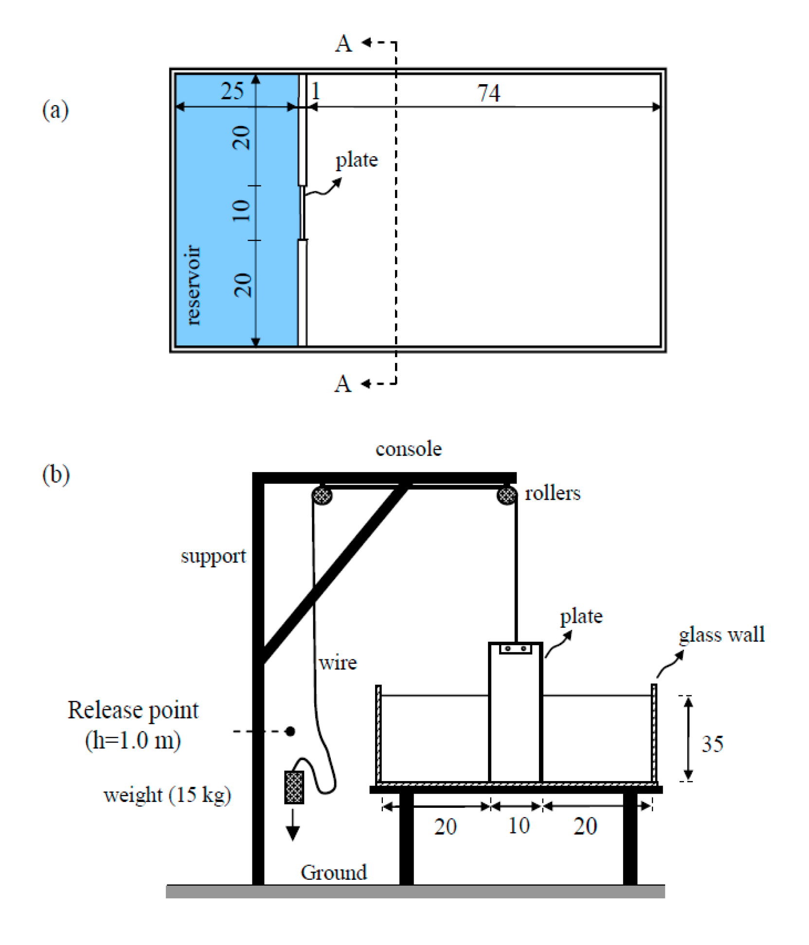
2.1. Experimental Setup

The experiments were carried out in the Hydraulic Laboratory of Civil Engineering at Iskenderun Technical University, Iskenderun, Turkey, in a small-scale rectangular horizontal channel with the following dimensions: 1.00 m length, 0.50 m width, and 0.35 m height (Figure 1a). The channel bottom and walls were made of a 9-mm thick glass. The reservoir was set upstream, covering 0.25 m of the channel, closed by two symmetric 0.20-m wide impermeable walls and by a 4 mm thick and 0.10 m wide plate coated with aluminum and made of rigid plastic representing the dam. The partial hole of the dam was simulated by the fast complete plate opening (Figure 1b). First, a steel rope was connected to the plate top. Then, the rope was drawn over a pulley with a 15 kg weight hanging at the other end. By releasing the weight from 1.0 m above the floor, the plate was removed in about 0.04 s, an opening time shorter than the one recommended by Hager and Lauber (1998) for a ‘sudden removal’, equal to 1.25(h₀/g)^1/2 (where h₀ is the reservoir depth, and g is the acceleration due to gravity) and corresponding to 0.15 s in the present tests.

2.2. Performed Tests

A total of three tests were conducted for both dry and wet conditions. The initial reservoir water depth was equal to h₀ = 0.15 m in all tests, whereas the tailwater depths h_d were 0.00 (dry condition) and 0.015 m and 0.030 m (wet conditions), respectively. The depth ratio α = h_d /h₀, calculated by dividing the tailwater depth h_d by the initial reservoir depth h₀, is, respectively, equal to 0.0, 0.1, and 0.2. Test conditions are synthetically resumed in

Table 1. List of performed tests.

TEST	hd [m]	α
D1	0.00	0
W1	0.015	0.1
W2	0.030	0.2

.

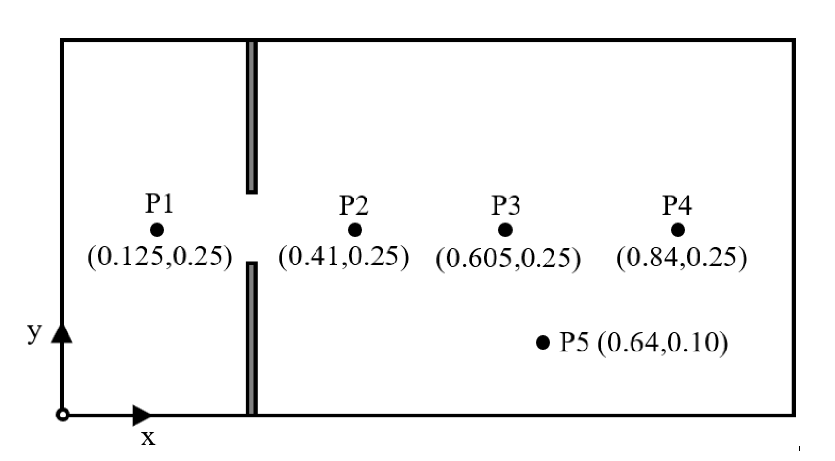
2.3. Measurement Technique

The fast evolution of the dam-break flow was recorded through a Sony Nex-7 camera with a 50-fps acquisition frequency at 1920 × 1080p resolution, positioned with the field of view focused on the downstream part of the channel. The reservoir water was colored using methylene blue dye [12]. The whole channel was lighted with fluorescent lamps located at the bottom. To better control the ambient light, tests were performed in a dark room, all of the sides of the channel were coated with black materials to reduce light reflection, and a white sheet of Plexiglas was put under the glass bottom.

Ultrasonic distance sensors (UDS) were used to obtain the time evolution of the water levels (i.e., the stage hydrographs). They measure distances by sending acoustic waves and measuring their return time [58,59,60,61,62]. Specifically, five Microsonic^TM sensors were used in the present study (one Mic+35/IU/TC and four Mic+25/IU/TCs). Measurement locations of the sensors are shown in Figure 2. The Mic+35/IU/TC sensor (P1) was used to obtain the water level variation upstream of the gate, since it has a higher measurement range (6.5–35 cm) and a slower response time (64 ms). The four Mic+25/IU/TC sensors (P2–P5) were used downstream in order to be able to measure fast water level changes, due to their lower measurement range (3–25 cm) and quicker response time (32 ms). More information about the UDS can be found in previous studies [63].

3. Numerical Model

With modern computing advancements, CFD has emerged as a robust hydraulic design and simulation tool. The commercially available CFD program FLOW-3D, developed by Flow Science Inc., Los Alamos NM [25], was used herein to simulate the dam-break wave propagation in an enclosed domain over both dry and wet beds. FLOW-3D, designed to treat time-dependent flow problems in one, two, and three dimensions, is claimed to apply to almost any type of flow and provides many options for users, including different numerical approaches. Specifically, in this work, the RANS equations with the k-ε model for the turbulence closure and SWEs were solved using the VOF (Volume of Fluid) technique for the free-surface flow simulation [22].

3.1. RANS Equations with k-ε Turbulent Model

The governing mass and momentum equations for Newtonian, incompressible fluid flow, which constitute the RANS equations, are expressed as below:

$$\frac{\partial }{\partial x_i}\left(u_i{A}_i\right)=0$$

(1)

$$\frac{\partial u_{ii}}{\partial \mathrm{t}}+\frac{1}{V_F}\left(u_j{A}_j\frac{\partial u_i}{\partial x_j}\right)=-\frac{1}{\rho }\frac{\partial p}{\partial x_i}+G_i+f_i$$

(2)

where x_i, i = 1,…, 3 represents the coordinate along the i-th direction in space, u_i (x_i, t_i) is the velocity, A_i is the fractional area open to flow over the i-th direction, t is time, V_F is the fractional volume open to flow, p is pressure, ρ is the fluid density, G_i represents the gravity accelerations, and f_i is the i-th component of the viscous acceleration term, expressed as follows:

$$r{V}_F{f}_i={\tau }_{b,i}-\frac{\partial }{\partial x_j}\left(A_j{\tau }_{ij}\right),$$

(3)

in which ${\tau }_{b,i}$ represents the wall shear stress, and $\tau$ the shear stress, given by:

$${\tau }_{ii}=2\mu \left\{\frac{\partial u_i}{\partial x_i}-\frac{1}{3}\left(\frac{\partial u_j}{\partial x_j}\right)\right\}, \mathrm{and} {\tau }_{ij}=-\mu \left\{\frac{\partial u_j}{\partial x_i}+\frac{\partial u_i}{\partial x_j}\right\} ,$$

(4)

with $\mu$ as the dynamic viscosity.

Wall boundary conditions are evaluated differently according to the chosen turbulence method, which uses a law of the wall formulation. In the present study, the standard k-ε turbulence closure was adopted, as was done in previous works involving rapidly varied high-Reynolds unsteady flows [16,25,26], in order to calculate the turbulence eddy viscosity with the turbulence kinetic energy k and the turbulent dissipation rate ε per unit fluid mass.

The Volume-of-fluid (VOF) method was used to detect the free-surface water profile. Grid cells are classified as full, empty, or partially filled with fluid, through a number between 0 and 1 for the free water surface in each cell, which is a fraction of water F, equal to 1 when the cell is completely filled with water and to 0 when the cell is completely empty. The VOF function F(x_i, t) is defined using the following transport equation:

$$\frac{\partial F}{\partial \mathrm{t}}+\frac{1}{V_F}\left\{\frac{\partial }{\partial \mathrm{x}}\left(F{A}_i{u}_i\right)\right\}=0$$

(5)

With FLOW-3D, complex geometries can be efficiently modeled by partially blocking each cell in a rectangular mesh using the FAVOR (Fractional Area/Volume Obstacle Representation) technique. However, like other discrete methods, this method is affected by the resolution of the computational grid. With the improvement of the mesh resolution, the solid geometry is better represented. When the mesh cells are partially blocked by a solid object, each computational cell is represented by a single volume fraction (VF) and three area fractions (A_i). The VF indicates how much volume is occupied by fluid in the cell after subtracting the volume occupied by solids (if there are any). In this case, the fraction of each mesh cell face through which the fluid can flow were determined as area fractions. Volume fraction and the fractional areas for each cell was calculated by the preprocessor.

Numerical computations were carried out on a structured finite-difference grid. The grid was staggered so that while scalar quantities of the fluid such as pressure (p), density (ρ), viscosity (µ), gravitational acceleration (G_i), volume fraction (V_F), and fluid fraction (F) were computed at the cell centers Only vector and tensor quantities such as velocities (u_i) and areas (A_i) were taken into account at the cell faces. For equations density, dynamic viscosity and gravitational acceleration were known constants at solution initiation. Velocities, pressure, and VOF function F are the time and space-dependent unknowns that needed to be calculated at all grid cells for each time step. These unknowns and all other quantities were determined numerically using necessary initial and boundary conditions.

3.2. The Shallow Water Equations

The Shallow Water Equations (SWEs) were derived from the depth-averaged 3D incompressible Navier–Stokes equations, neglecting vertical acceleration and assuming hydrostatic pressure distribution.

The software FLOW-3D permits solving the non-conservative form of the two-dimensional (2D) SWEs (i.e., the depth-averaged continuity and momentum equations), respectively:

$$\frac{\partial \left(V_{F}F\right)}{\partial t}+\frac{\partial \left(u{A}_{x}F\right)}{\partial x}+\frac{\partial \left(v{A}_{y}F\right)}{\partial y}=0$$

(6)

$$\frac{\partial u}{\partial t}+\frac{1}{V_F}\left(u{A}_x\frac{\partial u}{\partial x}+v{A}_y\frac{\partial u}{\partial y}\right)=-\frac{1}{\rho }\frac{\partial p}{\partial x}+G_x+\frac{{\tau }_{b,x}}{\rho d}$$

(7)

$$\frac{\partial v}{\partial t}+\frac{1}{V_F}\left(u{A}_x\frac{\partial v}{\partial x}+v{A}_y\frac{\partial v}{\partial y}\right)=-\frac{1}{\rho }\frac{\partial p}{\partial y}+G_y+\frac{{\tau }_{b,y}}{\rho d}$$

(8)

where u and v are the depth-averaged velocities along the horizontal x and vertical y directions, respectively, A_x and A_y are the fractional areas open to flow, F is the fluid fraction, G_x and G_y are the body acceleration components, d is the water depth, and ${\tau }_{b,x}$ and ${\tau }_{b,y}$ [64] represent the bottom shear stress components.

The FAVOR and the VOF methods were used in the SWEs model of FLOW-3D for the geometry description and fluid interface tracking, respectively. The volume fraction variable V_F and the water fraction variable F were used to define a variable bottom contour and the fluid depth, respectively [46]. Equations (6)–(8) are expressed in terms of volume, area, and water fractions for flow in a single layer of control volumes used to apply VOF and FAVOR methods.

The pressure was calculated as:

$$p=p_0+\rho gH$$

(9)

where p₀ is the atmospheric pressure on the water-free surface and H is the elevation of the free surface above the grid bottom (i.e., the sum of the obstacle and water depths):

$$H=\left(1-V_F\right)\cdot \delta z+F\cdot V_F\cdot \delta z.$$

(10)

In the SWEs model, the vertical z-direction is assumed as shallow direction, along which two real cells are considered in each mesh block. The lower cell size $\delta z$ in the z-direction is defined as being large enough to contain any fluid depth occurring throughout the simulation. For turbulent flow, in the SWE model, the bottom shear stress is evaluated through a quadratic law as follows:

$${\tau }_{b,x}=-\rho C_{D}u\sqrt{u^2+v^2}, {\tau }_{b,y}=-\rho C_{D}v\sqrt{u^2+v^2}$$

(11)

where C_D represents the drag coefficient. This coefficient can be defined manually or calculated using the following equation based on the surface roughness height:

$$C_D={\left[\frac{\kappa }{B+\left( z_0/d\right)}\right]}^2,$$

(12)

in which $\kappa$ = 0.4 is the Von Karman constant, B = 0.71 and z₀ = k_s/30, with k_s the surface roughness. Many depth-averaged flow models use Manning coefficient n to calculate the bed shear stress in SWEs except for the FLOW-3D SWE model which uses drag coefficient C_D instead. Manning’s n was not available in the version of the FLOW-3D SWE model used in the present study. When needed, the relationship between drag coefficient and Manning coefficient C_D = (n²g)/d^1/3 can be utilized to switch between these two coefficients.

In numerical simulations, Equations (6)–(8) can be solved explicitly and implicitly.

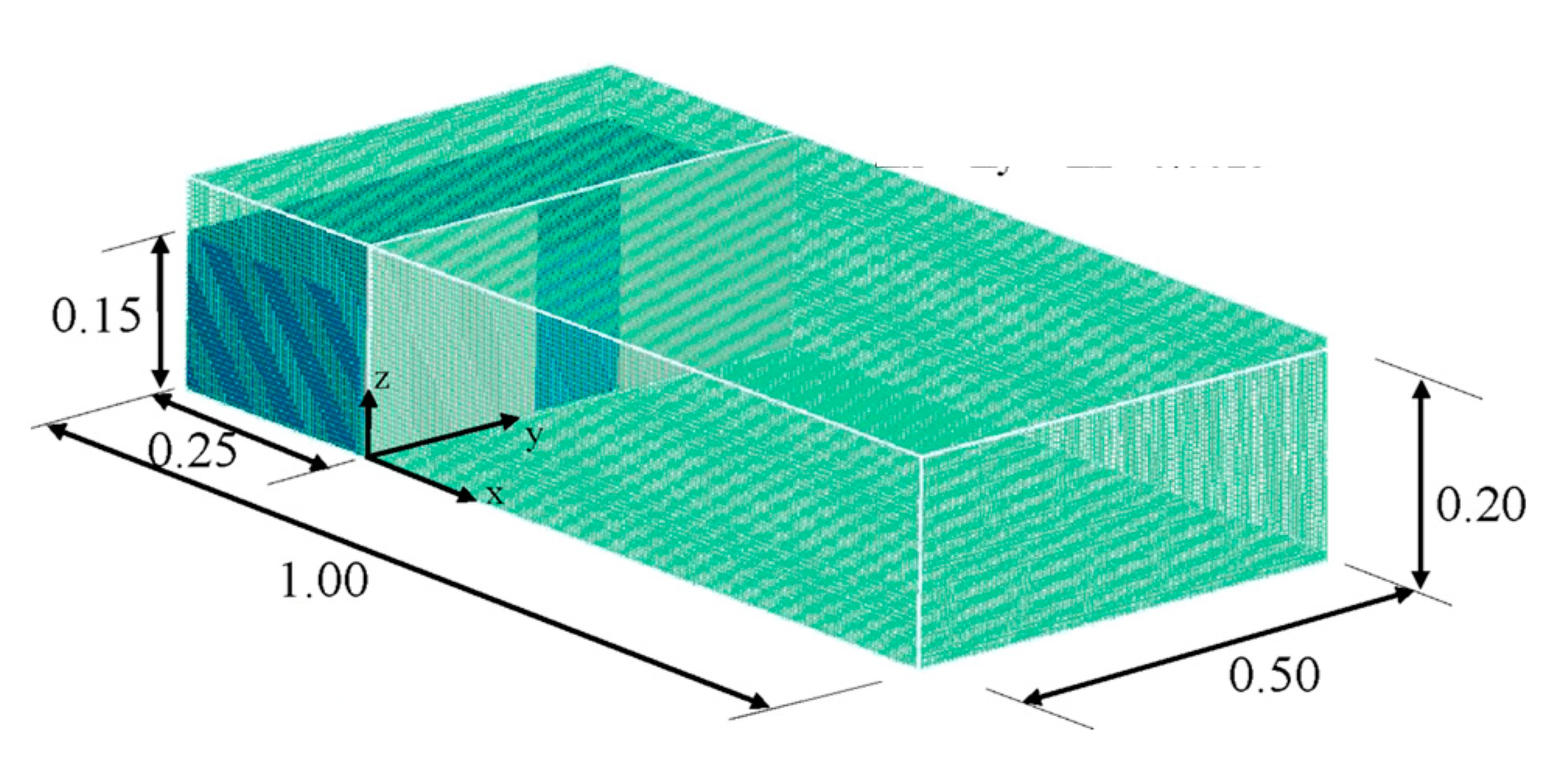
3.3. Solution Domain, Boundary and Initial Conditions

The computational domain (1.00 m long, 0.50 m wide, and 0.20 m high) was subdivided into a structured mesh of fixed square cells in all of the simulations. Herein, as mentioned before, a minimum of two real cells had to be defined in each mesh block in the z-direction in order to apply VOF in the SWEs model. The size of the lower layer cell in the z-direction had to be large enough to contain all the water in that layer through the simulation. The software allowed dividing z-axis horizontally into two layers, with a lower layer of 0.17 m and an upper layer of 0.20 m. After a sensitivity analysis, a uniform mesh size of 0.005 m was used in three directions in the 3D RANS model and in two directions for the SWEs model for the whole computational domain. The mesh resulted in 200, 100, and 40 cells in the x, y, and z directions, respectively (Figure 3). The total number of cells was therefore 800,000 for the RANS and 40,000 for the SWEs.

In the numerical computations, the sidewalls and the channel bottom were set as walls. At the top, over the air-water interface, the pressure boundary condition was assigned to account for the atmospheric pressure on the free surface. Since VOF defines the water surface, zero shear stress, and constant atmospheric pressure were applied [22]. A constant volume of fluid with dimensions of 0.25 × 0.50 × 0.15 m representing the reservoir was assigned as an initial condition (Figure 3). All channel walls were assumed to be smooth. The no-slip condition was defined as zero tangential and normal velocities.

Once the initial and boundary conditions were established, the model was applied to the three different above-described tailwater conditions (D1, W1 and W2). Simulations were run for a duration of t = 10 s for each scenario. The time step Δt was determined according to the Courant–Friedrichs–Lewy (CFL) condition. When rapidly varied unsteady flows, including strong hydraulic jump and wave breaking were modelled with SWEs in FLOW-3D, a second-order monotonicity preserving momentum advection approximation was used in order to provide robust and accurate results. For the RANS simulations, first-order momentum advection approximation was used. An implicit scheme was used to solve the equations in both numerical models. The drag coefficient C_D was taken as 0.025, 0.030, and 0.04 at SWEs simulations for D1, W1, and W2, respectively. Different C_D coefficients were used to obtain better results. The C_D coefficient significantly affected the reflected wavefront and water depths. The default drag coefficient value of 0.0026, or the one calculated with roughness height k_s for glass using Equation (11), did not give very good results in determining the water depths and wavefront velocity after wave reflection. This topic is also a subject of future study on dam-break flows with strong reflections causing turbulence and significant air entrainment.

4. Results

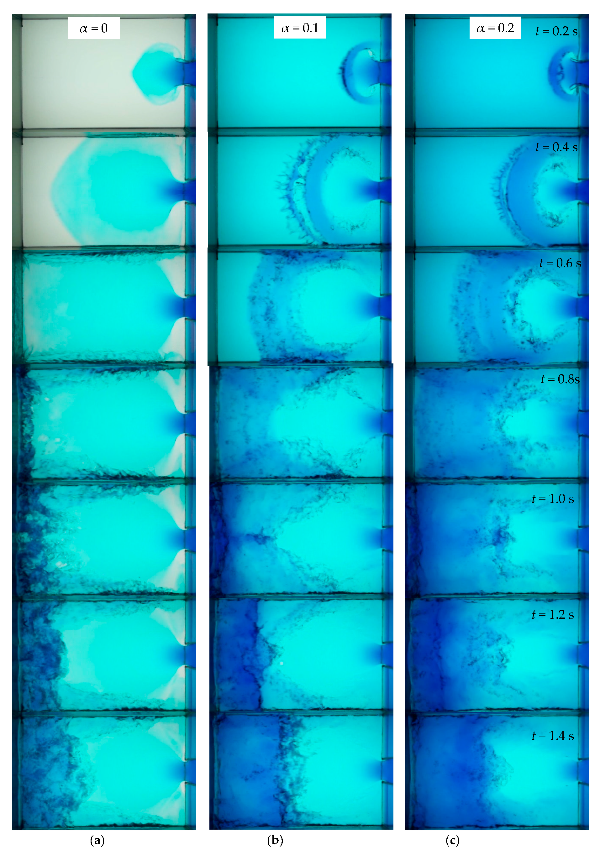
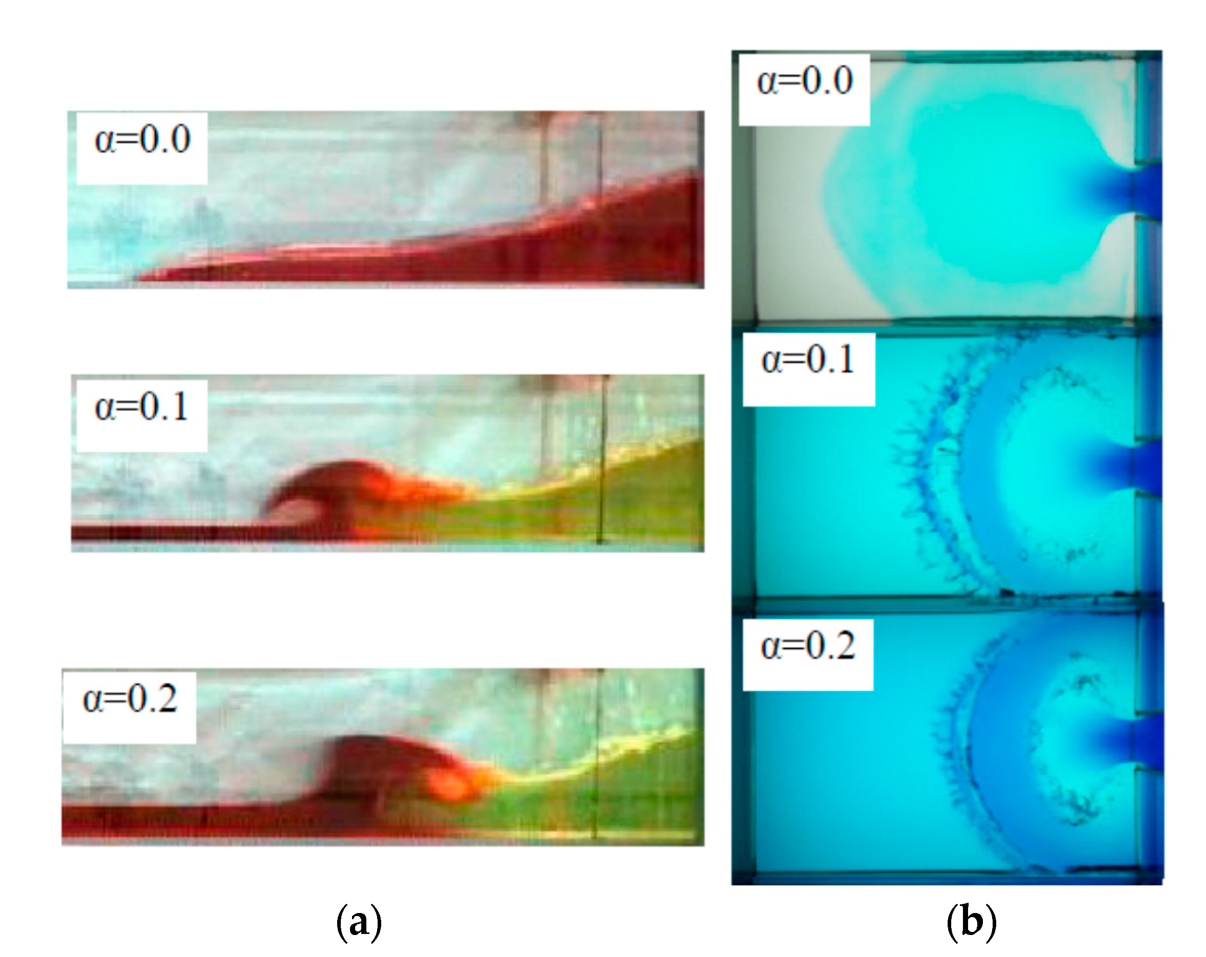
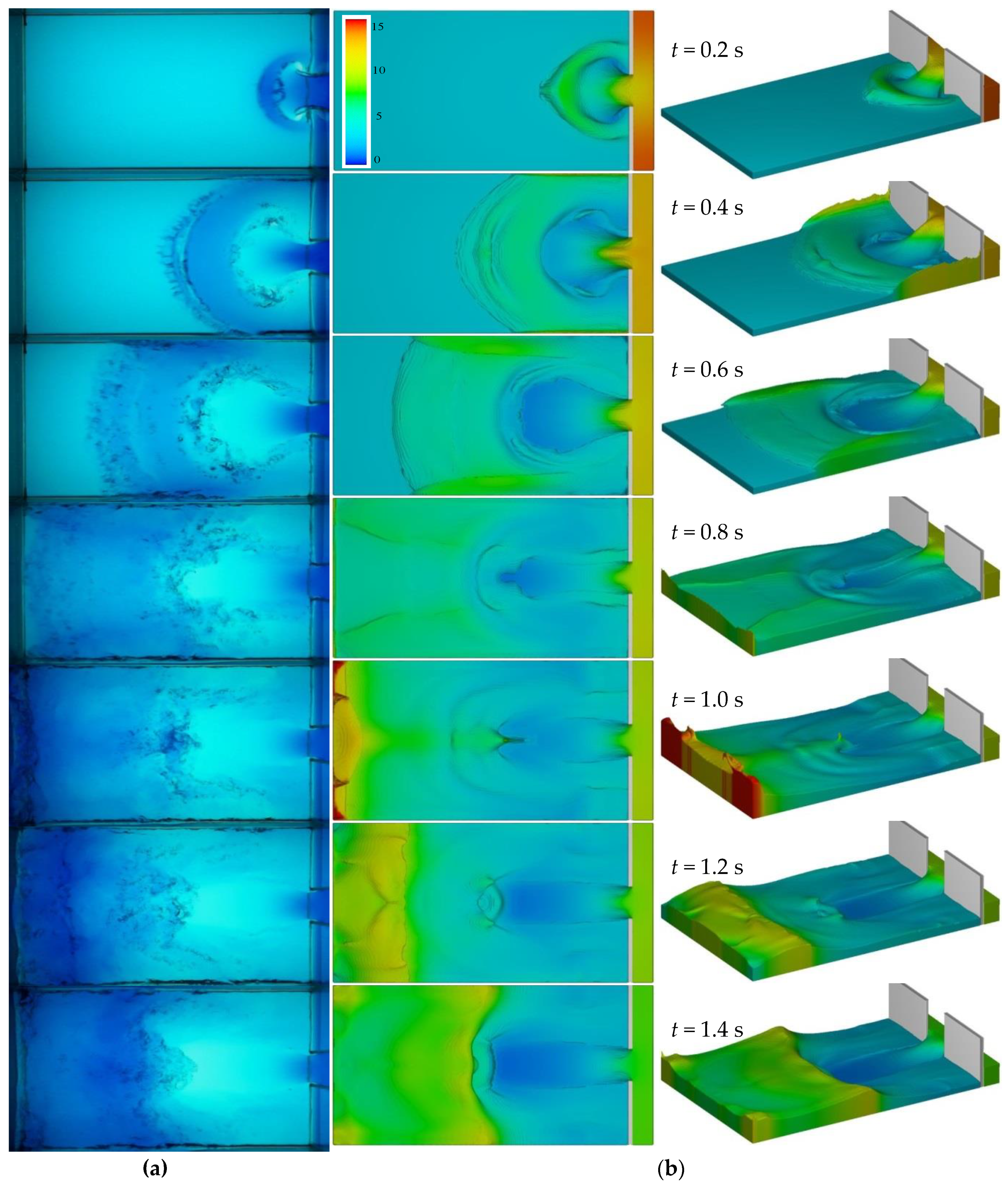
4.1. Experimental Results

Figure 4 shows video images from the top of the dam-break process evolution for tests D1 and W1-W2. After the sudden removal of the plate, the dam-break wave propagated downwards. As the wave reached the channel end wall, it reflected against it, locally increasing the flow depth, then resulting in a negative wave propagating upward. Differently from a 1D process, the wavefront also reflected against the channel sidewalls, and then oblique hydraulic jumps were formed. After the reflection, positive and negative waves keep propagating and overlapping in a complex way.

Additionally, the 3D test results were compared visually with the results of the 2D test performed by Kocaman and Ozmen-Cagatay [22] and Ozmen-Cagatay and Kocaman [52] in a channel with a rectangular cross section for the same depth ratios at the initial stages of the dam-break wave. In Figure 5, instead, the experimental results at time t = 0.4 s were plotted for all tests, comparing longitudinal and top views (2D and 3D experiments, respectively).

In the 2D experiments, the current wave confined within a rectangular channel can be simulated as propagating in one direction. However, in the scenarios considered here, where the dam hole (and consequently the initial cross-section of the wave) was smaller than the channel cross-section, the flow cannot be treated as 1D flow strictly with a preferential propagation direction. Due to the circular propagation and wave breaking in all directions, a 3D simulation was therefore necessary. A complex 3D flow, with strong turbulences and significant air entrainment, is in fact observed as a result of the reflection from the side and end walls of the channel in the 3D experiment.

Figure 4 and Figure 5 show that the dam-break wave propagates faster in dry bed conditions (test D1) than in the wet bed cases (tests W1 and W2). In addition, in this latter case, the wavefront velocity decreased as the tailwater depth increased. This may be explained by the higher resistance, due to the higher water depth encountered by the propagating waves. Soon after the plate removal, the reservoir water rushing out from the channel bottom uplifted the tailwater. In contrast, after the wave reflection, the front velocity became higher for tests W2 than for tests W1 and D1. This can be imputable to the higher impact velocity of the positive wave to the end wall, to the higher potential energy stored in the final part of the flume, and to the higher time lag in forming negative wave for the dry-bed case, as compared to the wet-bed cases (see, for example, times t = 0.6–1.2 s).

Moreover, a higher turbulence intensity with related significant energy dissipation was observed at the channel end for test D1 with respect to the wet-bed cases (see results for times t > 0.8 s in Figure 4). During the initial stages of the dam-break in the presence of tailwater, the pressure gradient forced the tailwater to move forward. Plunging-type wave breaking occurred, therefore, for the wet-bed tests, as shown in Figure 4 for t = 0.4 s and in Figure 5b. Accordingly, intensive turbulence appeared in the flow. As the tailwater depth increased (α = 0.4), spilling-type wave breaking occurred. It can also be noticed that the positive wave broke earlier as the tailwater decreased, as observed in Figure 4 and Figure 5.

Figure 4 and Figure 5 show, again, that there is a significant difference in wavefront velocities between dry and wet-bed cases. Specifically, the wavefront velocity was higher for the dry-bed case, with an average value of about 1.7 m/s. In contrast, the average value was about 0.9 m/s for tests W1 and W2, and it decreased with an increasing depth ratio (α). Similar behavior patterns were also observed in the 2D experimental dam-break studies conducted by [23] in a rectangular horizontal channel (Figure 5a).

The aforementioned observations indicate that the flow behavior at the downstream of the channel was very complex in an enclosed domain, involving multiple wave interactions. This kind of experimental study can be helpful in validating numerical models.

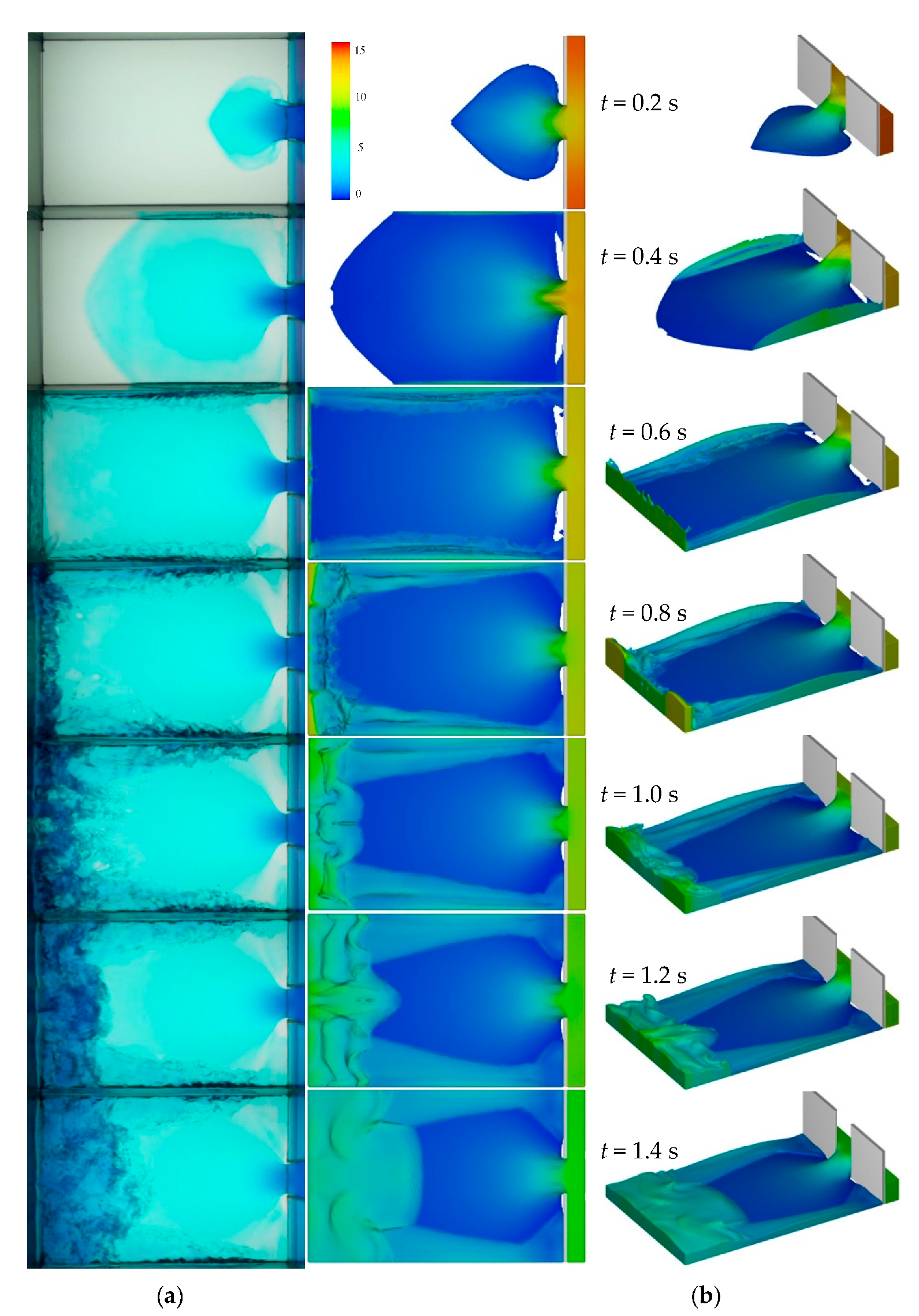
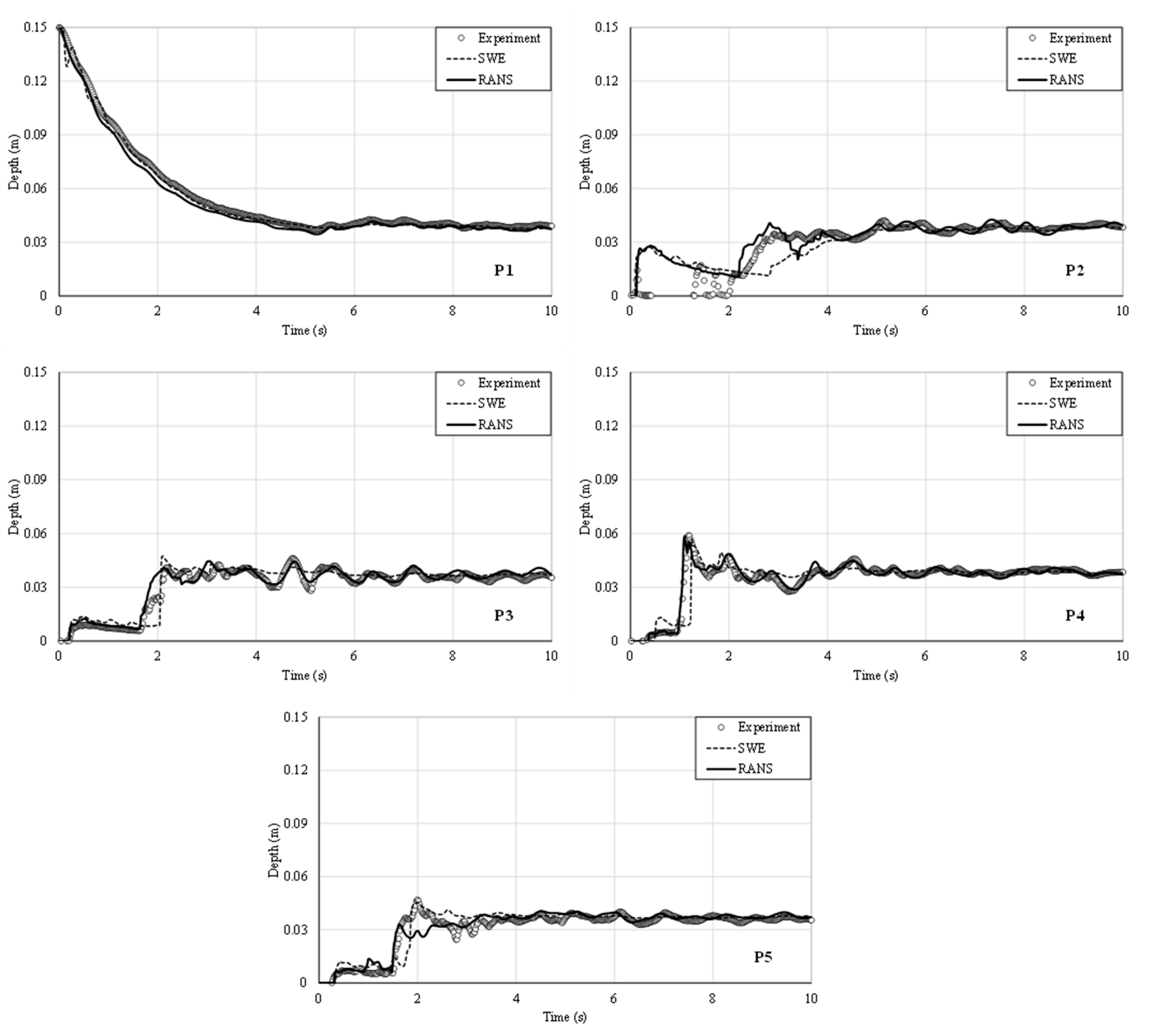
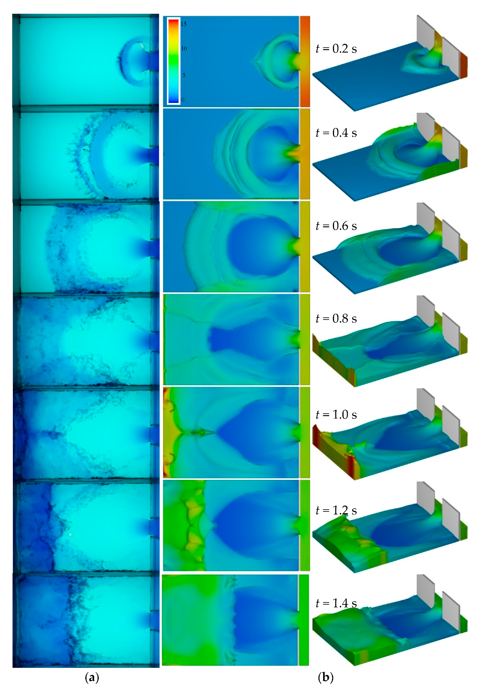
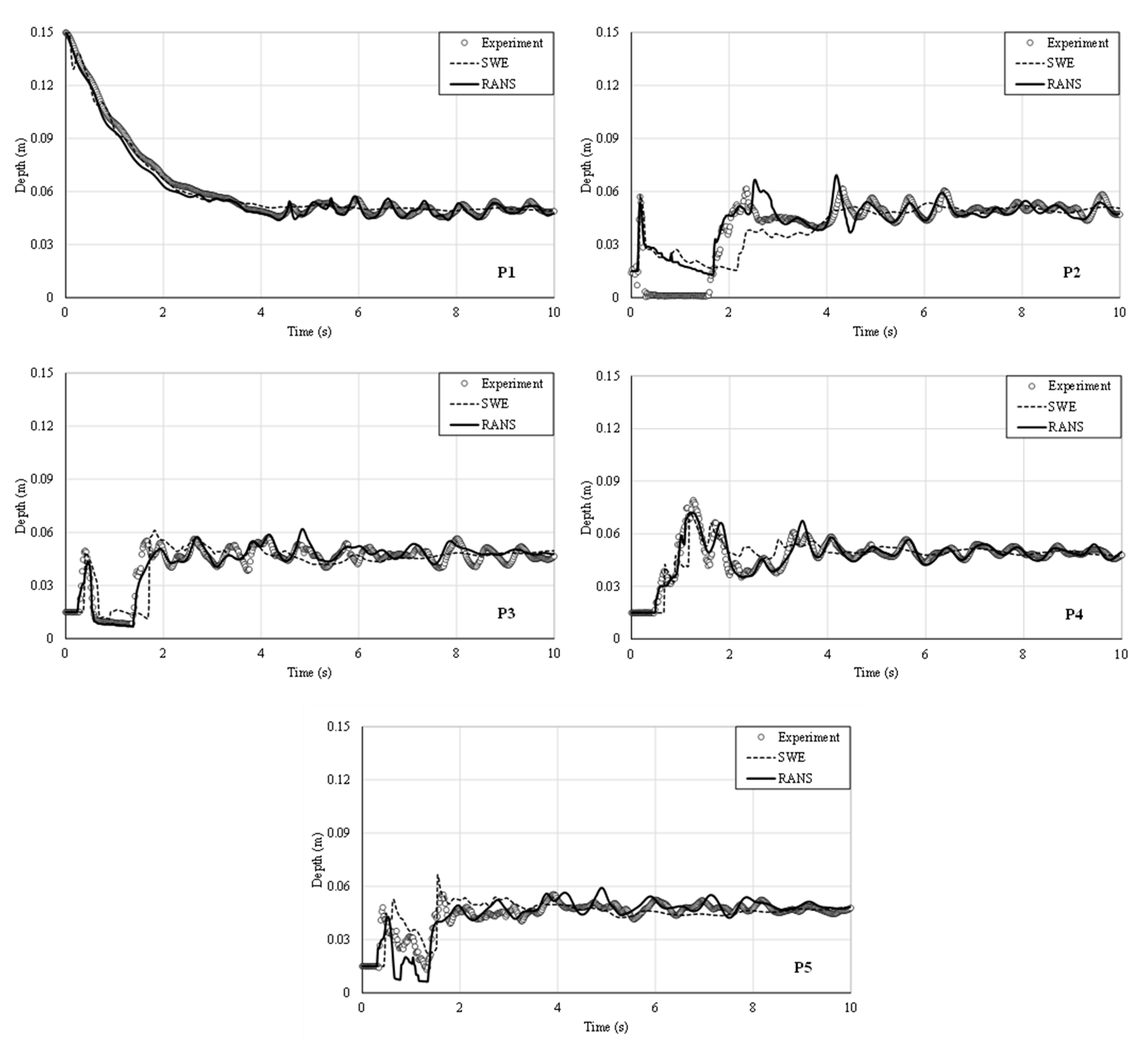
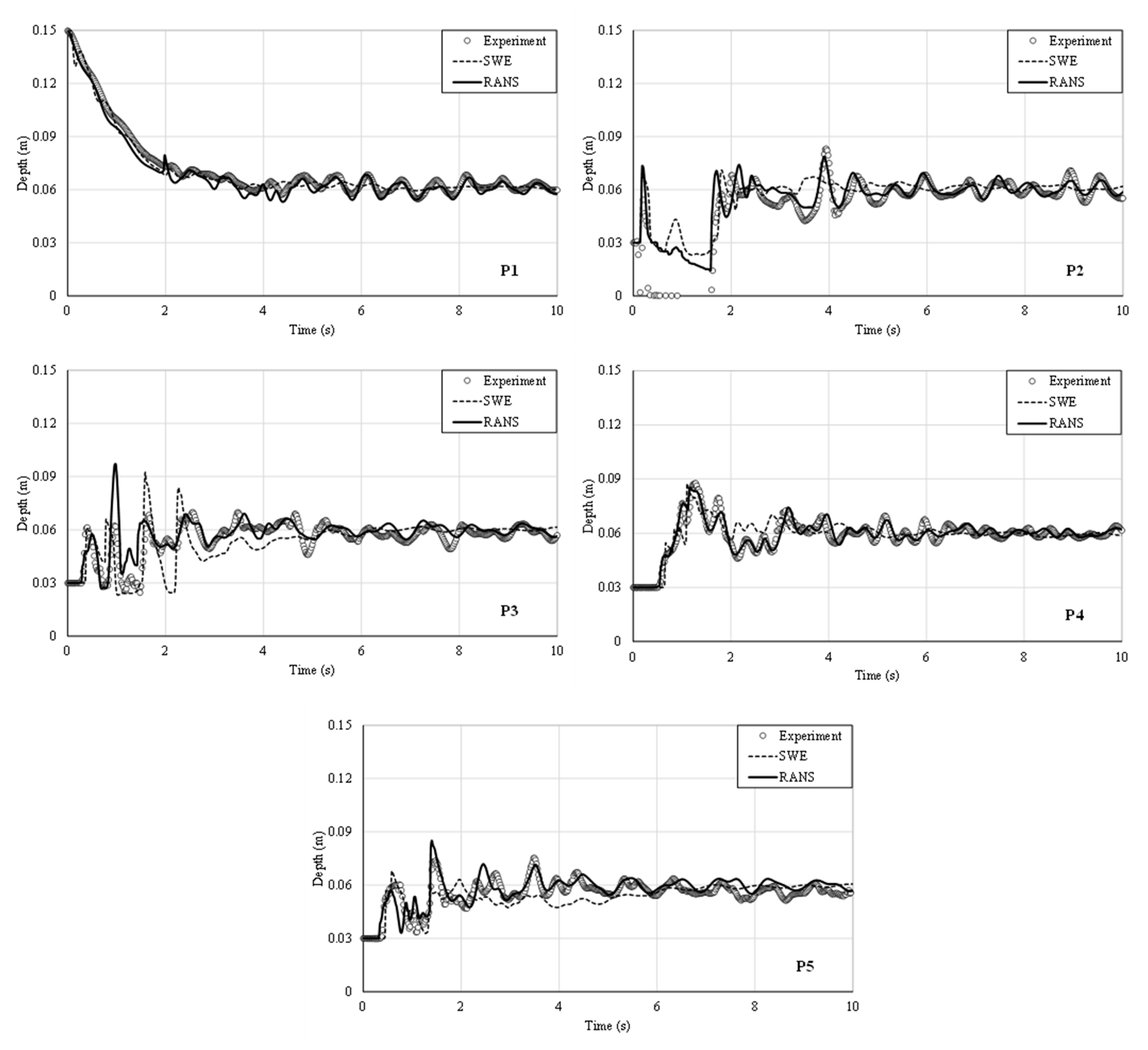
4.2. Comparison between Measured and Computed Results

Figure 6, Figure 7, Figure 8, Figure 9, Figure 10 and Figure 11 show the comparison between the experimental data and the numerical results of the dam-break process evolution for tests D1 and W1-W2, respectively. In Figure 6, Figure 8 and Figure 10, the experimental results are displayed on the left-hand side of each figure. The second and third columns refer, instead, to the numerical results calculated by the RANS.

A very good agreement between experimental data and the numerical simulation results can be observed for all tests D1 and W1-W2. Therefore, FLOW-3D can predict the dam-break wave propagation with acceptable accuracy in an enclosed domain over both dry and wet beds.

Numerical simulations have also been performed using SWEs. However, some differences can be noticed between the results obtained through the two different numerical schemes. As expected, the SWEs achieved a smaller accuracy than the RANS.

The stage hydrographs of the numerical (RANS and SWEs) and experimental results (P1–P5 sensors) for test D1 are given in Figure 7.

After the sudden removal of the gate, the water in the upstream tank moved instantly to the downstream channel and the water level fell rapidly at P1 for both experimental and numerical results until approximately t = 5.5 s. After that, the water level increased slightly due to the reflected wavefront and remained constant with minor fluctuations. A small disagreement occurred at P1 for all phases between experimental and numerical results.

It should be considered that P2 sensor graphs in all of the experiments gave erroneous results between the 0–2 s time interval, as the sensor could not read depths. This is because the waves reflected from the water surface could not reach the sensor. The response time of the sensor and curves of the flow surface were considered probable causes of the disagreement mentioned above. It is also noticeable that the SWE results were below the RANS and experimental results for time interval 2–4 s at P2, as the reflected wave passed this measurement point.

As for the P3 sensor, the experimental data are in agreement with the numerical data for time interval 0–1 s, while a disagreement was observed until t = 4 s. The water level slightly raised immediately after the sudden removal of the gate, and a sharp rise was observed in the SWE results as soon as the reflected wave reached the P3 (t = 0–2 s). After that, both the experimental and RANS results were in good agreement generally, while small oscillations due to reflections of the negative waves from the flume walls were not well represented by the SWE (t = 2–8 s). In addition, it was observed that the reflected wave celerity of the SWE results was slower than the experimental and RANS results at P3 and P4. The highest water level for the D1 case occurred at P4, located at the downstream end, as expected and already noticeable in Figure 6. Although arrival times of the reflected wave for the experimental and RANS results were quite similar, the RANS results were not as in good agreement with the experimental results as for the other probes, and the peak level of the water was not determined by the RANS at P5 (t = 2 s). Also, actual oscillations were not detected by both the computational methods (t = 3 s), and the reflected wave celerity of the SWE was slower than the other results, similar to P3 and P4. Nonetheless, the results agreed progressively with decreasing undulation after t = 4 s.

Figure 8 shows the comparison between the experimental data and the numerical results of the dam-break process evolution for test W1. The experimental results are displayed on the left-hand column, whereas the second and third columns refer to the numerical results calculated by the RANS.

A comparison of the stage hydrographs for the test case W1 is shown in Figure 9. After the fast removal of the sluice gate, water in the reservoir hit the tailwater and the flood wave moved downstream rapidly with a plunging type wave breaking that caused a complex flow behavior on the free surface. Significant fluctuations were observed on the surface with reflection phenomena of propagating waves from the side and the front-end wall of the channel, while also interacting with the incoming flow. It can be said that with the presence of the tailwater, more undulation occurred than D1 at all probes. The water level decreased quickly with the abrupt removal of the gate, and fluctuations occurred when the negative wavefront reached the P1. It can be noticed that the water depths predicted by the RANS simulations were lower than the experimental results for the time interval t = 0–3 s, which indicated that the discharge time of the upstream was not computed correctly by the RANS. After the discharge finished, the results agreed well at P1, proving that the RANS simulated the undulations properly. Also, it can be seen that the SWE discharged the upstream faster than other results at the initial phase until approximately t = 0.1 s. Then a peak was observed, the water level increased, and the SWE results agreed with the experimental results.

Nonetheless, undulations were not well determined by the SWE, unlike the RANS. A peak was observed at the beginning of the P2 and P3 plots due to passing breaking waves, then a gradual decrease occurred in the experimental and computed results due to the finite reservoir volume. The measurement method failed for P2 (t = 0–2 s). After that, the water level increased with the reflected wave and a hydraulic jump occurred in the RANS and measured results, unlike SWE. The hydraulic jump was later than in reality, which means that the SWE underestimated the jump’s velocity at P2 (t = 2–4 s). The agreement of the results increased with the decreasing oscillation for the rest of the plot. The behavior at the initial phase of the P3 sensor was similar to the P2 one, and the measured results were more successful. The hydraulic jump occurred just as for the previous probe. However, an almost 25% difference was calculated between the hydraulic jump heights of the two numerical results (t = 2 s). More undulations were observed compared to the P2 sensor, and the SWE results appeared inconsistent with the RANS and the experimental results (especially on the determination of the wave crests). Although there were some differences in the wave height and wave celerity at the P4 sensor, the measured and computed results were generally in better agreement compared to the other downstream probes in the W1 case. In contrast, the results were quite in disagreement at the P5 sensor for the time interval t = 0–2 s. Three different peak levels were observed at that time interval, and the discrepancy between the results was dramatic. Also, for the same time interval, the RANS and SWE water depths were lower and higher than the experimental results, respectively, showing the great difference between their theoretical approaches for complex flow conditions due to the collision of the moving and reflected wave at the end of the tank. In this region, the height of the hydraulic jump was not well determined by both the numerical methods, and the oscillations were not represented by the RANS as good as they were for previous probes (t = ~2–10 s).

Figure 10 shows the comparison between the experimental data (on the left-hand side) and the numerical results calculated by the RANS (second and third columns) of the dam-break process evolution for test W2. From the visual comparison, it is can be clearly stated that there is a good agreement between the experimental and numerical results.

The stage hydrographs for the test case W2 are shown in Figure 11. It is noticeable that the wave crests are sharper than for the W1 test, and the strong wave breaking cannot be seen here since the tailwater is higher in W2 test. It can be said that an increasing tailwater level, with constant initial reservoir water depth, caused sharper wave crests and less wave break. Similar behavior was observed in an earlier study [22]. The agreement of the SWE results with the measured results was better than the RANS at P1 before t = 4 s. With the increasing undulations the SWE results disagreed with both the RANS and the experimental results. Although the sharp crests were occasionally predicted nearly as measured, the SWE generally produced straight lines for the undulations in all cases of the present study due to neglecting the vertical velocity components and assuming hydrostatic pressure distribution in this model. Similar behaviors with the previous test case were observed at the P2 sensor, especially on the failed measurement results for t = 0–2 s. While the RANS and experimental results were in good agreement after the t = 2 s (except for the prediction of the wave crest at t = 4 s) the SWE determined the average water level almost properly.

The numerical results disagreed with the experimental results at the initial phase of the P3 plot, predicting the wave crest height 30% more than in reality for different time steps (t = 0–2 s). After that, the SWE results were below the other results until approximately t = 5 s. Then agreement increased, and less undulations were observed compared to the P3 sensor of the W1 test case. Even though many undulations occurred, P4 had the best agreement between the results, owing to the lower wave heights for the W2 among the downstream probes. However, the SWE disagreed with the other results for the time interval t = 2–3 s. The levels of the peaks were determined better than W1 at the P5 generally, whereas undulations were not well represented in terms of time steps of the wave crests. Although the comparison results are in good agreement overall, it can be said that the celerity of the small waves was not computed precisely by both numerical methods at this point.

The discrepancies between experimental and numerical models can be summed up in

Table 2. MAPE (Mean Absolute Percentage Error) error analysis referred to the comparison between numerical (RANS and SWEs, respectively) and experimental results for water level time histories at measurement points P1, P3, P4, and P5.

	P1		P3		P4		P5
	RANS	SWEs	RANS	SWEs	RANS	SWEs	RANS	SWEs
D1	5.17	2.91	9.45	14.74	4.99	12.57	12.54	15.37
W1	3.99	4.01	8.08	16.71	4.42	9.03	10.79	11.50
W2	3.90	3.84	8.83	13.01	3.63	7.16	8.16	10.67

in terms of the MAPE (Mean Absolute Percentage Error) of water level time histories in measuring points P1, P3, P4, and P5. The P2 error calculations in the table were not reported in the table, because, as explained before, the P2 sensor gave erroneous results between the 0–2 s time interval in all experiments, as it could not read water depths.

In general, the error rates in the SWEs were higher than the RANS for all of the simulations. As mentioned above and observed in Figure 7, Figure 9 and Figure 11, the highest errors were observed during the passage of the reflected wave for all cases (e.g., 12.54% for the RANS and 15.37% for the SWEs in test D1). The smallest error rates were observed at P1 located in the reservoir for the SWEs and the RANS (e.g., 3.99% for the RANS and 4.01% for the SWEs in test D1).

As expected, although the SWEs still appear as a well-established choice and most of the existing models developed to solve these equations can produce valuable results for flood prediction, they are not as efficient in simulating the observed dam-break wave propagation process in complex flows due to turbulence, air entrainment, hydraulic jumps, etc., which cannot be reproduced with hydrostatic pressure acceptance and shock wave representation. A 3D approach is to be preferred, at least with the RANS.

The present work investigates the capability and the performance of the two models to simulate dam-break flows in an enclosed domain with both dry and wet cases. It can be observed that the solution obtained from the VOF-based RANS numerical model reproduces, with reasonable accuracy, the propagation of the negative wave induced by the strong reflection of the dam-break flow against the side and end walls of the channel, though requiring a higher computational time. On the contrary, the SWEs simulations provided results which had little disagreement with the observed ones but with the advantage of less computational time, which would be even more significant in real-case and/or real-scale applications. As an example, considering the case W1, the run-time was approximately 2 min for the SWEs and 116 min for the RANS for a 10 s solution time, respectively, running the simulation a computer with an Intel Core i7 2.8 GHz 16 GB RAM. Hence, SWE-based numerical models are still preferable over RANS-based models for problems requiring large computational domains, especially where the vertical acceleration is insignificant due to fewer computational efforts and time. Usually, fine meshes are needed in numerical simulations in order to better represent irregular topographies and obtain more accurate results. On the other hand, more computational time and effort are required for 3D solutions of real-case dam-break problems in the presence of large-scale artificial or natural obstacles such as buildings, bridges, levees, and canopies [51]. In order to analyze the flow characteristics around 3D structures (i.e., bridges) using fine mesh to capture localized flow details, the hybrid models combining RANS-based 3D flow and SWEs models in one simulation can also be used to reduce the computation time [25].

5. Conclusions

This paper presents a 3D experimental and numerical investigation of the dam-break wave propagation during its initial stages in an enclosed domain over dry and wet beds with two different tailwater levels. Image processing for flow measurements yields 3D unsteady flow behavior economically and straightforwardly during the laboratory tests.

The findings show a significant difference in the propagation of wavefronts between the dry and wet domains. The velocity of the wavefront was faster for dry-bed conditions than the wet-bed cases. In addition, as the tailwater depth increased, the wavefront velocity decreased. This is due to the higher resistance of the higher water depth to the propagating waves. However, after reflection from the downstream wall, the wavefront velocity of the negative wave increased as the depth ratio increased. During the early dam-break stages, intense turbulence was observed for the dry-bed case. This turbulence, generated from the bottom friction, caused a significant energy dissipation on the channel end wall. Also, in the wet-bed cases, early wave breaking caused turbulence and energy dissipation in the domain. Therefore, as the depth ratio decreases, wave breaking occurred earlier.

The measured results were then compared with those of numerical simulations, and reasonable agreements were achieved. Herein, the CFD package, FLOW-3D, produced good results in predicting the 3D dam-break flow propagation in an enclosed domain over dry and wet beds, both with the RANS and the SWEs. However, as expected, although the SWEs present the advantage of requiring less time and computational resources, their assumptions are not applicable at the initial stages of the dam-break and at the front of the dam-breaking wave and near structures (due to the highly transient nature of dam-break flows, the 3D effects, and the involved turbulence). The modeling of such complex flows should be based on 2D or 3D models that use the Navier–Stokes equations. SWEs are sufficient tools for predicting the water arrival at large time or far from the dam, but not to simulate high free-surface gradient flows or to calculate the pressure-load on structures. Fortunately, the increasing computational power provided by the recent multiprocessor computers and the access to modern massively parallel supercomputers allow for the resort to more complex 3D numerical models, which can more accurately reproduce the physical processes, when needed, and in real-scale cases.

In addition, despite the potential power of numerical simulations, physical models always constitute a useful tool to investigate different features under controlled conditions and to better understand several features of the physical processes, especially when complex real problems have to be simulated. The laboratory results presented here can be valuable to validate 3D numerical models or assist the design, due to difficulties in getting field data on dam-break flows.

References

1. Rendina, I.; Viccione, G.; Cascini, L. Kinematics of flow mass movements on inclined surfaces. Theor. Comput. Fluid Dyn. 2019, 33, 107–123. [Google Scholar] [CrossRef]
2. Evangelista, S.; Altinakar, M.S.; Di Cristo, C.; Leopardi, A. Simulation of dam-break waves on movable beds using a multi-stage centered scheme. Int. J. Sediment Res. 2013, 28, 269–284. [Google Scholar] [CrossRef]
3. Pohle, F.V. Motion of Water Due to Breaking of a Dam and Related Problems; USNBS: Washington, DC, USA, 1952; pp. 47–53. [Google Scholar]
4. Kosorin, K. Hydraulic characteristics of some dam-break wave singularities. In Proceedings of the 20th IAHR Congress, International Association for Hydraulic Research, Moscow, Russia, 5–9 September 1983; pp. 520–528. [Google Scholar]
5. Stoker, J.J. Water Waves. In Water Waves; Wiley: Hoboken, NJ, USA, 1992; pp. 291–449. [Google Scholar]
6. Ritter, A. Die Fortpflanzung der Wassarwellen, Z. Vereines Deutsh. Ing. 1892, 36, 947–954. [Google Scholar]
7. Dressler, R.F. Comparison of theories and experiments for the hydraulic dam-break wave. In Assoc Int d’Hydrol Sci, Assemblee Generale De Rome, 1st ed.; National Bureau of Standards: Washington, DC, USA, 1954; Volume 38, pp. 319–328. [Google Scholar]
8. Whitham, G.B. The effects of hydraulic resistance in the dam-break problem. In Proceedings of the Royal Society of London. A. Mathematical and Physical Sciences; The Royal Society: London, UK, 1955; Volume 227, Issue 1170; pp. 399–407. [Google Scholar] [CrossRef]
9. Schmidgall, T.; Strange, J.N. Floods Resulting from Suddenly Breached Dams. Conditions of High Resistance. Hydraulic Model Investigation; Army Engineer Waterways Experiment Station: Vicksburg, MS, USA, 1961; Miscellaneous Paper N. 2-374; Available online: https://apps.dtic.mil/dtic/tr/fulltext/u2/268411.pdf (accessed on 3 August 2020).
10. Bellos, C.V.; Soulis, V.; Sakkas, J.G. Experimental investigation of two-dimensional dam-break induced flows. J. Hydraul. Res. 1992, 30, 47–63. [Google Scholar] [CrossRef]
11. Bell, S.W.; Elliot, R.C.; Chaudhry, M.H. Experimental results of two-dimensional dam-break flows. J. Hydraul. Res. 1992, 30, 225–252. [Google Scholar] [CrossRef]
12. Fraccarollo, L.; Toro, E.F. Experimental and numerical assessment of the shallow water model for two-dimensional dam-break type problems. J. Hydraul. Res. 1995, 33, 843–864. [Google Scholar] [CrossRef]
13. Lauber, G.; Hager, W.H. Experiments to dambreak wave: Horizontal channel. J. Hydraul. Res. 1998, 36, 291–307. [Google Scholar] [CrossRef]
14. Stansby, P.K.; Chegini, A.; Barnes, T.C.D. The initial stages of dam-break flow. J. Fluid Mech. 1998, 374, 407–424. [Google Scholar] [CrossRef]
15. Bukreev, V.I.; Gusev, A.V. Initial stage of the generation of dam-break waves. Dokl. Phys. 2005, 50, 200–203. [Google Scholar] [CrossRef]
16. Korobkin, A.; Yilmaz, O. The initial stage of dam-break flow. J. Eng. Math. 2008, 63, 293–308. [Google Scholar] [CrossRef] [Green Version]
17. Leal, J.G.A.B.; Ferreira, R.M.L.; Cardoso, A.H. Dambreak waves on movable bed. In Proceedings of the River Flow 2002, Louvain-la-Neuve, Belgium, 4–6 September 2002; Bousmar, D., Zech, Y., Eds.; Balkema: Rotterdam, The Netherlands, 2002; Volume 2, pp. 981–990. [Google Scholar]
18. Di Cristo, C.; Evangelista, S.; Greco, M.; Iervolino, M.; Leopardi, A.; Vacca, A. Dam-break waves over an erodible embankment: Experiments and simulations. J. Hydraul. Res. 2017, 56, 196–210. [Google Scholar] [CrossRef]
19. Soares-Frazao, S.; Zech, Y. Experimental study of dam-break flow against an isolated obstacle. J. Hydraul. Res. 2007, 45, 27–36. [Google Scholar] [CrossRef]
20. Ozmen-Cagatay, H.; Kocaman, S. Experimental study of tail water level effects on dam-break flood wave propagation. In Proceedings of the International Conference River Flow 2008, Cesme, Turkey, 3–5 September 2008; Al-tinakar, M.S., Kokpinar, M.A., Aydin, I., Cokgor, S., Kirkgoz, S., Eds.; Volume 1, pp. 635–644, ISBN 978-605-60136-1-4. [Google Scholar]
21. Aureli, F.; Maranzoni, A.; Mignosa, P.; Ziveri, C. An image processing technique for measuring free surface of dam-break flows. Exp. Fluids 2010, 50, 665–675. [Google Scholar] [CrossRef]
22. Kocaman, S.; Ozmen-Cagatay, H. Investigation of dam-break induced shock waves impact on a vertical wall. J. Hydrol. 2015, 525, 1–12. [Google Scholar] [CrossRef]
23. Amicarelli, A.; Manenti, S.; Albano, R.; Agate, G.; Paggi, M.; Longoni, L.; Mirauda, D.; Ziane, L.; Viccione, G.; Todeschini, S.; et al. SPHERA v.9.0.0: A Computational Fluid Dynamics research code, based on the Smoothed Particle Hydrodynamics mesh-less method. Comput. Phys. Commun. 2020, 250, 107157. [Google Scholar] [CrossRef]
24. Crespo, A.; Domínguez, J.; Rogers, B.; Gómez-Gesteira, M.; Longshaw, S.; Canelas, R.; Vacondio, R.; Barreiro, A.; García-Feal, O. DualSPHysics: Open-source parallel CFD solver based on Smoothed Particle Hydrodynamics (SPH). Comput. Phys. Commun. 2015, 187, 204–216. [Google Scholar] [CrossRef]
25. Flow Science, Inc. FLOW-3D® Version 11; Flow Science, Inc.: Santa Fe, NM, USA, 2019. [Google Scholar]
26. BOSS International, BOSS DAMBRK. Hydrodynamics Flooding Routing User’s Manual; BOSS International, BOSS DAMBRK: Madison, WI, USA, 1999. [Google Scholar]
27. HEC-RAS. River Analysis System. US Army Corps of Engineers. Hydrologic Engineering Center. Hydraulic Reference Man-ual. Version 5.0. 2016. Available online: https://www.hec.usace.army.mil/software/hec-ras/documentation/HEC-RAS%205.0%20Reference%20Manual.pdf (accessed on 17 June 2021).
28. Toro, E.F. Riemann Solvers and Numerical Methods for Fluid Dynamics; Springer Science and Business Media LLC: Berlin, Germany, 2009. [Google Scholar]
29. LeVeque, R.J. Finite Volume Methods for Hyperbolic Problems; Cambridge University Press: Cambridge, UK, 2002; Volume 31. [Google Scholar]
30. Lai, J.-S.; Lin, G.-F.; Guo, W.-D. An upstream flux-splitting finite-volume scheme for 2D shallow water equations. Int. J. Numer. Methods Fluids 2005, 48, 1149–1174. [Google Scholar] [CrossRef]
31. Aliparast, M. Two-dimensional finite volume method for dam-break flow simulation. Int. J. Sediment Res. 2009, 24, 99–107. [Google Scholar] [CrossRef]
32. Ahmada, M.F.; Mamat, M.; Wan Nik, W.B.; Kartono, A. Numerical method for dam break problem by using Godunov approach. Appl. Math. Comp. Intel. 2013, 2, 95–107. [Google Scholar]
33. Mirauda, D.; Albano, R.; Sole, A.; Adamowski, J. Smoothed Particle Hydrodynamics Modeling with Advanced Boundary Conditions for Two-Dimensional Dam-Break Floods. Water 2020, 12, 1142. [Google Scholar] [CrossRef] [Green Version]
34. Viccione, G.; Bovolin, V. Simulating Triggering and Evolution of Debris-Flows with Smoothed Particle Hydrodynamics (SPH). Ital. J. Eng. Geo. Environ. 2011, 523–532. [Google Scholar] [CrossRef]
35. Ferrari, A.; Fraccarollo, L.; Dumbser, M.; Toro, E.F.; Armanini, A. Three-dimensional flow evolution after a dam break. J. Fluid Mech. 2010, 663, 456–477. [Google Scholar] [CrossRef]
36. Larocque, L.A.; Imran, J.; Chaudhry, M.H. 3D numerical simulation of partial breach dam-break flow using the LES and k–ϵ turbulence models. J. Hydraul. Res. 2012, 51, 145–157. [Google Scholar] [CrossRef]
37. Marsooli, R.; Wu, W. 3-D finite-volume model of dam-break flow over uneven beds based on VOF method. Adv. Water Resour. 2014, 70, 104–117. [Google Scholar] [CrossRef]
38. Issakhov, A.; Imanberdiyeva, M. Numerical Study of the Movement of Water Surface of Dam Break Flow by VOF Methods for Various Obstacles. Int. J. Nonlinear Sci. Numer. Simul. 2020, 21, 475–500. [Google Scholar] [CrossRef]
39. Wu, W.; Marsooli, R.; He, Z. Depth-Averaged Two-Dimensional Model of Unsteady Flow and Sediment Transport due to Noncohesive Embankment Break/Breaching. J. Hydraul. Eng. 2012, 138, 503–516. [Google Scholar] [CrossRef]
40. Wu, G.; Yang, Z.; Zhang, K.; Dong, P.; Lin, Y.-T. A Non-Equilibrium Sediment Transport Model for Dam Break Flow over Moveable Bed Based on Non-Uniform Rectangular Mesh. Water 2018, 10, 616. [Google Scholar] [CrossRef] [Green Version]
41. Rodi, W. Turbulence Modeling and Simulation in Hydraulics: A Historical Review. J. Hydraul. Eng. 2017, 143, 03117001. [Google Scholar] [CrossRef]
42. Shigematsu, T.; Liu, P.L.-F.; Oda, K. Numerical modeling of the initial stages of dam-break waves. J. Hydraul. Res. 2004, 42, 183–195. [Google Scholar] [CrossRef]
43. Yang, C.; Lin, B.; Jiang, C.; Liu, Y. Predicting near-field dam-break flow and impact force using a 3D model. J. Hydraul. Res. 2010, 48, 784–792. [Google Scholar] [CrossRef]
44. Ozmen-Cagatay, H.; Kocaman, S. Dam-Break Flow in the Presence of Obstacle: Experiment and CFD Simulation. Eng. Appl. Comput. Fluid Mech. 2011, 5, 541–552. [Google Scholar] [CrossRef] [Green Version]
45. Ozmen-Cagatay, H.; Kocaman, S. Investigation of Dam-Break Flow Over Abruptly Contracting Channel with Trapezoidal-Shaped Lateral Obstacles. J. Fluids Eng. 2012, 134, 081204. [Google Scholar] [CrossRef]
46. Hu, H.; Zhang, J.; Li, T. Dam-Break Flows: Comparison between Flow-3D, MIKE 3 FM, and Analytical Solutions with Experimental Data. Appl. Sci. 2018, 8, 2456. [Google Scholar] [CrossRef] [Green Version]
47. Munoz, D.H.; Constantinescu, G. 3-D dam break flow simulations in simplified and complex domains. Adv. Water Resour. 2020, 137, 103510. [Google Scholar] [CrossRef]
48. Kocaman, S.; Güzel, H.; Evangelista, S.; Ozmen-Cagatay, H.; Viccione, G. Experimental and Numerical Analysis of a Dam-Break Flow through Different Contraction Geometries of the Channel. Water 2020, 12, 1124. [Google Scholar] [CrossRef] [Green Version]
49. Brufau, P.; Garcia-Navarro, P. Two-dimensional dam-break flow simulation. Int. J. Numer. Meth. Fluids 2000, 33, 35–57. [Google Scholar] [CrossRef]
50. Wang, J.S.; Ni, H.G.; He, Y.S. Finite-Difference TVD Scheme for Computation of Dam-Break Problems. J. Hydraul. Eng. 2000, 126, 253–262. [Google Scholar] [CrossRef]
51. Quecedo, M.; Pastor, M.; Herreros, M.; Merodo, J.F.; Zhang, Q. Comparison of two mathematical models for solving the dam break problem using the FEM method. Comput. Methods Appl. Mech. Eng. 2005, 194, 3984–4005. [Google Scholar] [CrossRef]
52. Ozmen-Cagatay, H.; Kocaman, S. Dam-break flows during initial stage using SWE and RANS approaches. J. Hydraul. Res. 2010, 48, 603–611. [Google Scholar] [CrossRef]
53. Evangelista, S. Experiments and Numerical Simulations of Dike Erosion due to a Wave Impact. Water 2015, 7, 5831–5848. [Google Scholar] [CrossRef] [Green Version]
54. Mohapatra, P.K.; Eswaran, V.; Bhallamudi, S.M. Two-Dimensional Analysis of Dam-Break Flow in Vertical Plane. J. Hydraul. Eng. 1999, 125, 183–192. [Google Scholar] [CrossRef] [Green Version]
55. Alcrudo, F.; Garcia-Navarro, P. A high-resolution Godunov-type scheme in finite volumes for the 2D shallow-water equations. Int. J. Numer. Methods Fluids 1993, 16, 489–505. [Google Scholar] [CrossRef]
56. Kuiry, S.N.; Pramanik, K.; Sen, D. Finite Volume Model for Shallow Water Equations with Improved Treatment of Source Terms. J. Hydraul. Eng. 2008, 134, 231–242. [Google Scholar] [CrossRef]
57. Morris, M.W. CADAM-Concerted Action on Dam-Break Modelling; HR: Wallingford, UK, 2000. [Google Scholar]
58. Murzyn, F.; Chanson, H. Free-Surface, Bubbly Flow and Turbulence Measurements in Hydraulic Jumps. Research Report N° CH 63/07; Department of Civil Engineering, The University of Queensland: Brisbane, Australia, 2007; p. 118. ISBN 9781864998917. [Google Scholar]
59. Murzyn, F.; Chanson, H. Free-surface fluctuations in hydraulic jumps: Experimental observations. Exp. Therm. Fluid Sci. 2009, 33, 1055–1064. [Google Scholar] [CrossRef] [Green Version]
60. Chachereau, Y.; Chanson, H. Free-surface fluctuations and turbulence in hydraulic jumps. Exp. Therm. Fluid Sci. 2011, 35, 896–909. [Google Scholar] [CrossRef] [Green Version]
61. Kocaman, S.; Dal, K. A New Experimental Study and SPH Comparison for the Sequential Dam-Break Problem. J. Mar. Sci. Eng. 2020, 8, 905. [Google Scholar] [CrossRef]
62. Dal, K.; Kocaman, S. Comparison of the experimental results with SPH method for sequential dam-break problem. In Proceedings of the 5th IAHR Europe Congress, Trento, Italy, 12–14 June 2018. [Google Scholar]
63. Munir, M.M.; Salam, R.A.; Widiatmoko, E.; Supriadani, Y.; Rahmadhani, A.; Latief, H.; Khairurrijal, K. Web-Based Surface Level Measuring System Employing Ultrasonic Sensors and GSM/GPRS-Based Communication. Appl. Mech. Mater. 2015, 771, 92–95. [Google Scholar] [CrossRef]
64. Fiorentino, A.; De Luca, G.; Rizzo, L.; Viccione, G.; Lofrano, G.; Carotenuto, M. Simulating the fate of indigenous antibiotic resistant bacteria in a mild slope wastewater polluted stream. J. Environ. Sci. 2018, 69, 95–104. [Google Scholar] [CrossRef]
Figure 1. Schematic view of experimental setup and plate removal mechanism: (a) Plan and (b) A-A cross-section. Lengths are in [cm].
Applsci 11 05638 g001
Figure 2. Measurement points.
Applsci 11 05638 g002
Figure 3. 3D configuration of the numerical model for the RANS simulations (dry case).
Applsci 11 05638 g003
Figure 4. Comparison of tailwater depth effect on wave propagation for tests (a) D1, (b) W1, and (c) W2.
Applsci 11 05638 g004
Figure 5. Dam-break wave propagation for all tests at t = 0.4 s: (a) 2D experiments [22,52] and (b) 3D experiments.
Applsci 11 05638 g005
Figure 6. Comparison between experimental (a) and numerical results (b) for test D1 (α = 0).
Applsci 11 05638 g006
Figure 7. Comparison of experimental and numerical stage hydrographs (P1–P5 sensors) for test D1.
Applsci 11 05638 g007
Figure 8. Comparison between experimental (a) and numerical (b) results for test W1 (α = 0.1).
Applsci 11 05638 g008
Figure 9. Comparison of experimental and numerical stage hydrographs (P1–P5 sensors) for test W1.
Applsci 11 05638 g009
Figure 10. Comparison between experimental (a) and numerical (b) results for test W2 (α = 0.2).
Applsci 11 05638 g010
Figure 11. Comparison of experimental and numerical stage hydrographs (P1–P5 sensors) for test W2.
Applsci 11 05638 g011