Performance Characterization of a New Model for a Cyclone Separator of Particles Using Computational Fluid Dynamics

Abstract

In the present study, through Computational Fluid Dynamics techniques, the performance characterization of a new Stairmand-type separator cyclone was carried out using the commercial software ANSYS Fluent. Four models for the geometrical cyclone separator were built, namely model A as per the dimensions reported in the literature and models B, C, and D by applying square and circular shape cavities as a passive flow control technique on the surface of its cylindrical section. The Navier-Stokes equations with the RSM turbulence model were formulated to solve the continuous phase of the cyclone separator and, the Lagrangian approach was adopted to track the solid particles with one way-coupling. The proposed model’s separation efficiency and pressure drop were compared against those recorded in the previous studies reported in the literature. Model D was the cyclone separator that stood out as the most valuable by demonstrating a separation efficiency and pressure drop decrement of 0.42% and 6.01%, respectively.

1. Introduction

Air pollution is defined as the presence of gases and small particles in the air that are conducive to health risks of people and the environment [1]. These particles, known as particulate matter, are a set of solid and/or liquid particles suspended in air, coming from natural or anthropogenic sources [2]. Particulate matter is one of the most researched environmental pollutants worldwide because it is associated with cardiovascular, cardiac, and respiratory illnesses [2,3,4,5]. Particulate matter is also highly hazardous for people with chronic illnesses, pregnant women, senior citizens, and children [6,7,8]. Nowadays, millions of dollars are invested search alternatives to control and mitigate air pollution. Consequently, numerous studies show that the cyclone separator is adequate equipment that produces good results and represents part of the broad range of emission control devices [9].

Cyclone separators are mechanical collectors whose primary function is to separate solid particles from a gas using centrifugal force [10]. This particulate matter collection equipment is the most used device in all industrial areas (energy, chemical, and cement, among others) because its simple design is absent of moving parts, which results in low maintenance costs. This indicates that it can be used under a broad range of operational conditions [11,12].

The beginning of the cyclone operation deals with the gas tangentially entering the cyclone. Subsequently, the gas descends in a spiral pattern toward the bottom of the cone as a result of the cyclone geometry. Following this flow pattern, the particle matter is separated from the gas and moves towards the cyclone walls, where it strikes and loses kinetic energy, falling to the bottom of the conical section. Finally, the gas rises in a second spiral with a smaller diameter than the initial spiral and exits the top of the cyclone through a vertical duct known as the vortex finder [13,14].

Issues revolving around the separation efficiency and the pressure drop are the most important parameters to keep in mind during the design process of cyclone separators. In such a case, there are different physical and geometrical variables that directly come into play in association with these two parameters that include the density of the particles, the viscosity of the gas, the geometrical dimensions of the cyclone, the cut-off diameter of the particles, the inlet velocity, etc. On this basis, numerous studies have been conducted to research and analyze the different variables (mentioned above) that contribute to the performance of the cyclones [9,15]. Many documents show the different structural differences in cyclone separators, the most notable are those proposed by Stairmand, Lapple, Swift, and Linoya [12,16].

Hoffman et al. [17] experimentally analyzed the effects of the length of the cyclone separator in the performance of the equipment. The author found that the length of the cylindrical section of the cyclone affects its performance greatly; by increasing the length by a range of 2.65 to 5.5 times the diameter of the cyclone, the value of the separation efficiency elevates, and the pressure drop diminishes. Furthermore, another group of researchers analyzed the influence that the gas inlet section had on the performance of the cyclone separator. Zhao et al. [18] compared the performance of three cyclone designs having different geometry in their inlet section. The first design had a tangential inlet, the second design had a direct spiral inlet, and the third design had a symmetrical convergent spiral inlet. The collective results confirmed that the convergent spiral inlet possessed a better performance when compared to the other designs. On the other hand, Elsayed and Lacor [19] using the RSM turbulence model, computationally evaluated the effect that the geometry of the inlet section of the cyclone has upon the separation efficiency. The authors found that an augmentation in the dimensions of the cyclone inlets resulted in an attenuation in its performance.

Additionally, the literature portrays research referring to the effects that the conical section has on the performance of the cyclone separator. To that effect, Chuah et al. [16] simulated the performance of three cyclones using CFD, each cyclone with different diameters in the bottom of the cone. The simulations revealed that a decrease of size to the lower diameter of the conical section resulted in an increase in the separation efficiency and the pressure drop. Interestingly, the aforementioned study could contradict the work presented by Elsayed and Lacor [20], who researched the effect that the diameter of the bottom of the cone has on the performance of three cyclone separators. The authors concluded that the diameter of the tip of the cone has an insignificant effect on the performance of the cyclone. However, Xiang et al. [21] determined that the size of the cone has a significant effect on the performance of the cyclone if its opening is greater compared to the diameter of the vortex finder.

In terms of the vortex finder, the literature exposes certain differences that have had effects on the geometry of the exit duct. Regarding this aspect, Hoekstra [22] conducted an experiment using cyclones with smaller diameters in their vortex finder. The author found that the cyclones with less small diameter in their vortex finder conveyed a cutback in the cyclone’s central vortex, as well as a boost in the separation efficiency. Additionally, the research objective of El-Batsh [23] was to optimize the dimensions of the vortex finder. Five models of cyclone separators were tested in the study; each model had a unique geometrical configuration in its vortex finder. Results established that an increase in the diameter of the exit duct causes reductions in efficiency and in the pressure drop. Moreover, Xiang and Lee [24] and Brar et al. [14] have validated the impact of the diameter of the vortex finder. The authors found the relationship between the diameter of the vortex finder and the efficiency parameters of the cyclone. If this is the case, a reduction in the diameter of the exit duct leads to increments in the efficiency of separation and pressure drop of the cyclone concurrently.

In reference to the background previously stated, it is possible to conceive part of the progress developed during the last few years in order to continually improve the characteristics of the equipment. However, despite all this progress, there are many avenues of improvement that can be applied to these devices that have not been examined as of today. One of these possibilities is the use of passive flow control techniques, like the ones proposed in [25,26,27,28,29,30,31,32,33,34,35]. The contribution of this research is framed in the use of Computational Fluid Dynamics (CFD) to describe a new cyclone separator model with geometrical changes based on passive flow control techniques. To do so, three geometrical models were built, for which, their separation efficiency and pressure drop will be determined and evaluated to establish the new cyclone model.

2. Specifics of the Base Cyclone Model and Validation

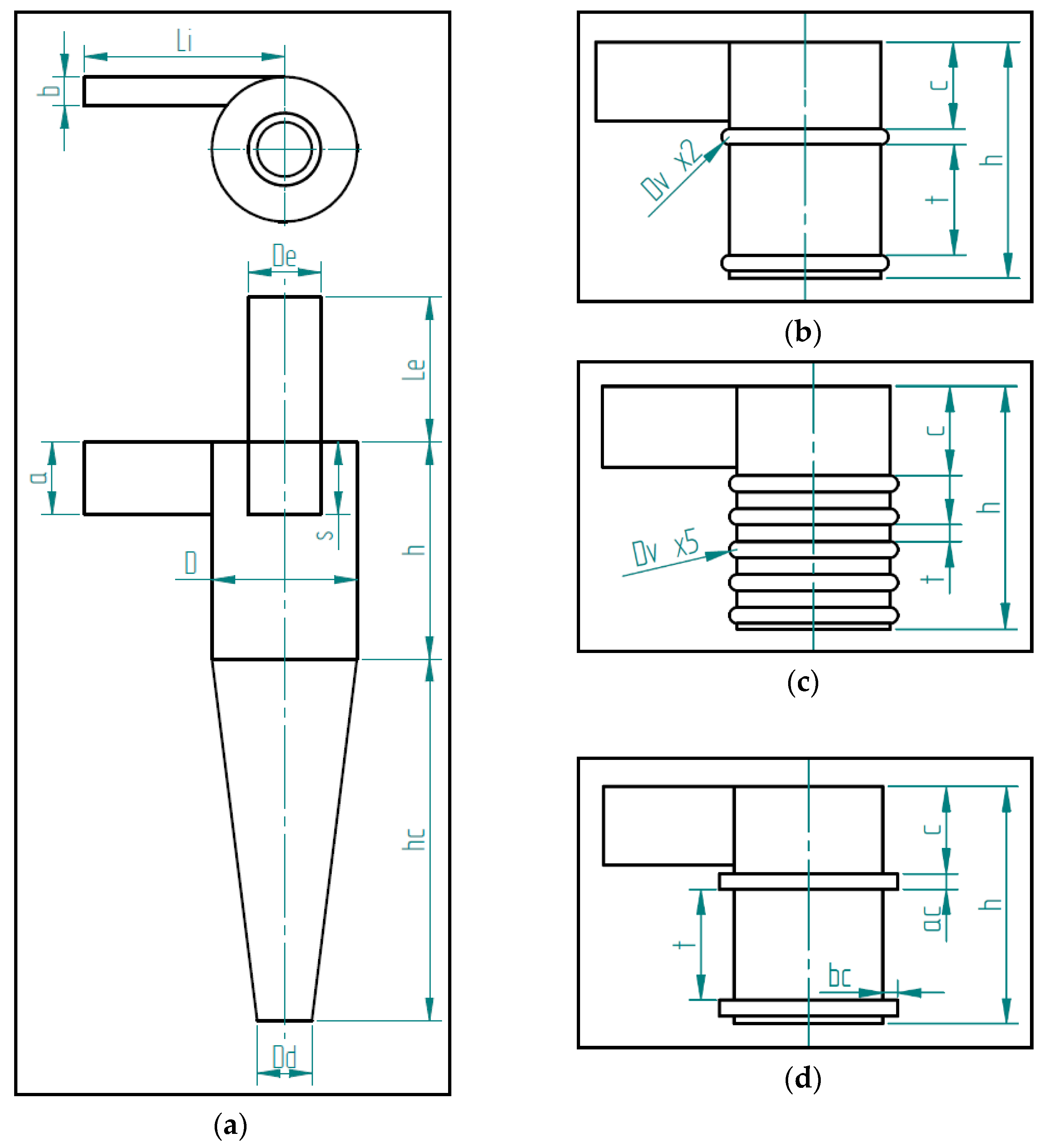
The Stairmand high-efficiency cyclone separator was the base and validation model selected for this research [36] because it is the base design for most of the work aimed at optimizing and building new cyclone models [10,11,12]. The information referring to the dimensions of the Stairmand high-efficiency cyclone model is listed in

Table 1. Geometrical details of the Stairmand high-efficiency particulate separator cyclone and the new particulate separator cyclone models based on passive flow control techniques.

Geometry	Symbol	Dimensions (mm)
		Model A	Model B	Model C	Model D
Cylinder length	h	435	435	435	435
Conical length	hc	725	725	725	725
Inlet height	a	145	145	145	145
Inlet width	b	58	58	58	58
Cylinder diameter	D	290	290	290	290
Cone apex diameter	Dd	109	109	109	109
Vortex Finder Diameter	De	145	145	145	145
Inlet length	Li	400	400	400	400
Vortex Finder Upper Section	Le	290	290	290	290
Vortex Finder Lower Section	s	145	145	145	145
Pitch	t	a Na	203	30	203
Cavity height	ac	a Na	a Na	a Na	29
Cavity width	bc	a Na	a Na	a Na	29
Cavity diameter	Dv	a Na	29	29	a Na
Distance from cyclone roof to cavity	c	a Na	160	160	160

^a Does not apply to this model.

and plotted in Figure 1.

For practical purposes, throughout this research the Stairmand high-efficiency cyclone will be called Model A, while cyclone separator models based on flow control techniques will be called models B, C, and D, respectively.

3. Flow Control

Flow control is defined as the process by which the flow configuration in a device, surface, structure, etc., is changed and/or manipulated in order to improve its performance [30]. Through the application of different flow control strategies and procedures, such as how to alter the transition point in the boundary layer, control fluid separation, and a contraction or escalation of the turbulence level of the fluid can be performed. From these changes, it is possible to obtain useful effects such as the alleviation in the dragging value, curtailment in noise indicators, raise in the lift value, as well as an increase in the mix rates and heat transfer. Flow control methods can be active or passive, the difference between the two concepts lies in that passive flow control does not require an external supply source or any feedback system, in comparison to active flow control, which requires the use of the system, supply sources or external controls to be applied [27,34]. During the last few years, numerous studies have been done [25,26,27,28,29,30,31,32,33,34,35] that are focused on the application of different flow control techniques in order to improve processes and/or industrial equipment, civil or military vehicles (land, air, and maritime), among others, to improve the economy as well as to protect the environment [30]. According to the aforementioned and using the studies published by [25,29,30] as a reference, this paper will apply cavity shaped as a passive flow control technique in the surface of the cylindrical section of the three cyclone separator models proposed.

Each of the aforementioned three models has a particular arrangement or cavity disposition. Therefore, the first cyclone model (model B) will have two circular cavities. The second model (model C) will have five circular cavities in its cylindrical section. And lastly, the third cyclone model (model D) will incorporate two square cavities in its design. Figure 1 and Table 1 show all the details of the newly proposed cyclone separator models.

4. Description of the Physical System

4.1. Navier Stokes Equations

The equations that describe the behavior of the continuous phase correspond to Navier Stokes equations. These equations model the mass and momentum conservation principles. Accordingly, considering that the fluid flow in the cyclone separator is stationary, tridimensional, highly turbulent, isothermal, and incompressible, the Navier Stokes equations could be expressed as:

$$\frac{\partial u_i}{\partial x_i}=0$$

(1)

$$\frac{\partial u_i}{\partial x_i}+u_j\frac{\partial u_i}{\partial x_i}=-\frac{1}{\rho }\frac{P}{\partial x_i}+v\frac{{\partial }^2{u}_i}{\partial x_i\partial x_j}-\frac{\delta }{\partial x_j}\left(\overline{u_i’u_j’}\right)$$

(2)

where $u_i$ is the average velocity of the fluid, $P$ is the average pressure of the fluid, $x_i$ is the spatial direction, $v$ is the kinematic viscosity, $\rho$ is the fluid density, and $\overline{u_i’u_j’}$ is the Reynolds stress tensor. In this study, Navier Stokes equations are solved by an Eulerian approach.

4.2. Turbulence Model

During the last few years, computational fluid dynamics has gained considerable recognition from many sectors (industrial, academic, among others), thanks to its ability to emulate the behavior of countless fluids that are present in real life using numeric simulations. The precision of the results in CFD is conditioned to the modeling of the case study and the choice of the ideal turbulence model to solve it.

The selection of the turbulence model is subject to the characteristics of the flow. In the case of the cyclone separators, the internal flow is complex since it is highly turbulent and anisotropic. Flow in the cyclones can be modeled by using commercial software, such as ANSYS Fluent [37], which has several turbulence models that go from the two equation models (k-ε standard and RNG) to the seven equations Reynolds Stress Model (RSM), and the large-scale model (LES). However, it should be considered that not all of these models properly solve the flow in cyclone separators. For example, equation models (k-ε standard and RNG) that are based on isotropic eddy viscosity are not suitable for cyclonic flows. In addition, researchers evaluated the performance of these turbulence models the moment they simulate the flow inside the cyclone. Results showed that the k-ε standard and RNG models cannot predict the complex periodic and tridimensional characteristics intrinsic to the internal flow in the cyclone separators [11]. Furthermore, the literature highlights numerous papers that have obtained good results when using the RSM turbulence model [10,14,16,20,38,39] and the LES model [40,41,42,43].

The RSM model with wall functions will be used for this study because it is able to predict the flow turbulence, as well as simulate factors such as the flow pattern, axial velocity, tangential velocity, pressure drop, and separation efficiency of the cyclone separator [19].

The transport equation for RSM is given as:

$$u_k\frac{\partial }{\partial x_i}\left(\overline{u_i’u_j’}\right)=D_{ij}+P_{ij}p+{\theta }_{ij}-{\epsilon }_{ij}$$

(3)

The diffusive transport term $D_{ij}$ is given as:

$$D_{ij}=-\frac{\partial }{\partial x_K}\left(\frac{D_t}{{\sigma }_k}\frac{\partial \overline{u_i’u_j’}}{\partial x_K}\right)$$

(4)

The stress generation term $P_{ij}$ is given as:

$$P_{ij}=-\rho \left(\overline{u_i’u_k’}\frac{\partial u_j}{\partial x_k}+\overline{u_j’u_k’}\frac{\partial u_i}{\partial x_K}\right)$$

(5)

The pressure strain correlation term ${\theta }_{ij}$ is given as:

$${\theta }_{ij}=P\overline{\left(\frac{\partial u{’}_i}{\partial x_j}+\frac{\partial u{’}_j}{\partial x_i}\right)}$$

(6)

The dissipation term ${\epsilon }_{ij}$ is given as:

$${\epsilon }_{ij}=2v\overline{\frac{\partial u{’}_i}{\partial x_k}}\overline{\frac{\partial u{’}_j}{\partial x_k}}$$

(7)

4.3. Governing Equations for the Dispersed Phase

Simulation of the flow laden with solid particles is developed through the Lagrangian+Eulerian approach. When the interaction between the continuous phase and the dispersed phase takes place, the dynamic interaction between both phases interact can be unidirectional or bidirectional. Because of the low volumetric fraction of the dispersed phase in this study case (3–5%), it is assumed that coupling between the phases is unidirectional (one-way coupling), the particles do not have a considerable effect on the physical properties of the fluid. According to this and keeping in mind that in Fluent [37], the Lagrangian approach is used to track the solid particles dispersed in the continuous phase, this study will use the Lagrangian approach. For just one disperse particle, the equilibrium equation is given as:

$$\frac{\partial u_{pi}}{dt}=F_D\left(u_i-u_{pi}\right)+\frac{\left({\rho }_{\rho }-\rho \right)g_i}{{\rho }_{\rho }}+F_i$$

(8)

where $u_{pi}$ is the velocity of the particles, $F_D\left(u_i-u_{pi}\right)$ is the drag force that acts over the particles, ${\rho }_{\rho }$is the density of the particles, $g_i$ is the gravitational acceleration, and $F_i$ corresponds to the additional forces that can act upon the particle, such as Brownian force, the Saffman and Magnus force, the added mass force, electromagnetic forces, and Basset force, among others; all these forces are expressed per mass unit. For spherical particles, drag force is given as:

$$F_D=\frac{18\mu }{{\rho }_{\rho }{d}_{\rho }{}^2}\frac{C_{D}Re}{24}$$

(9)

The Reynolds number is expressed as:

$$R_e=\frac{\rho d_{\rho }\left|u_p-u\right|}{\mu }$$

(10)

where $d_{\rho }$is the diameter of the particle, $u$is the velocity of the fluid, $u_p$ is the velocity of the particle, $\rho$ is the density of the fluid, and $\mu$ is the dynamic viscosity of the fluid.

4.4. Mesh Generation

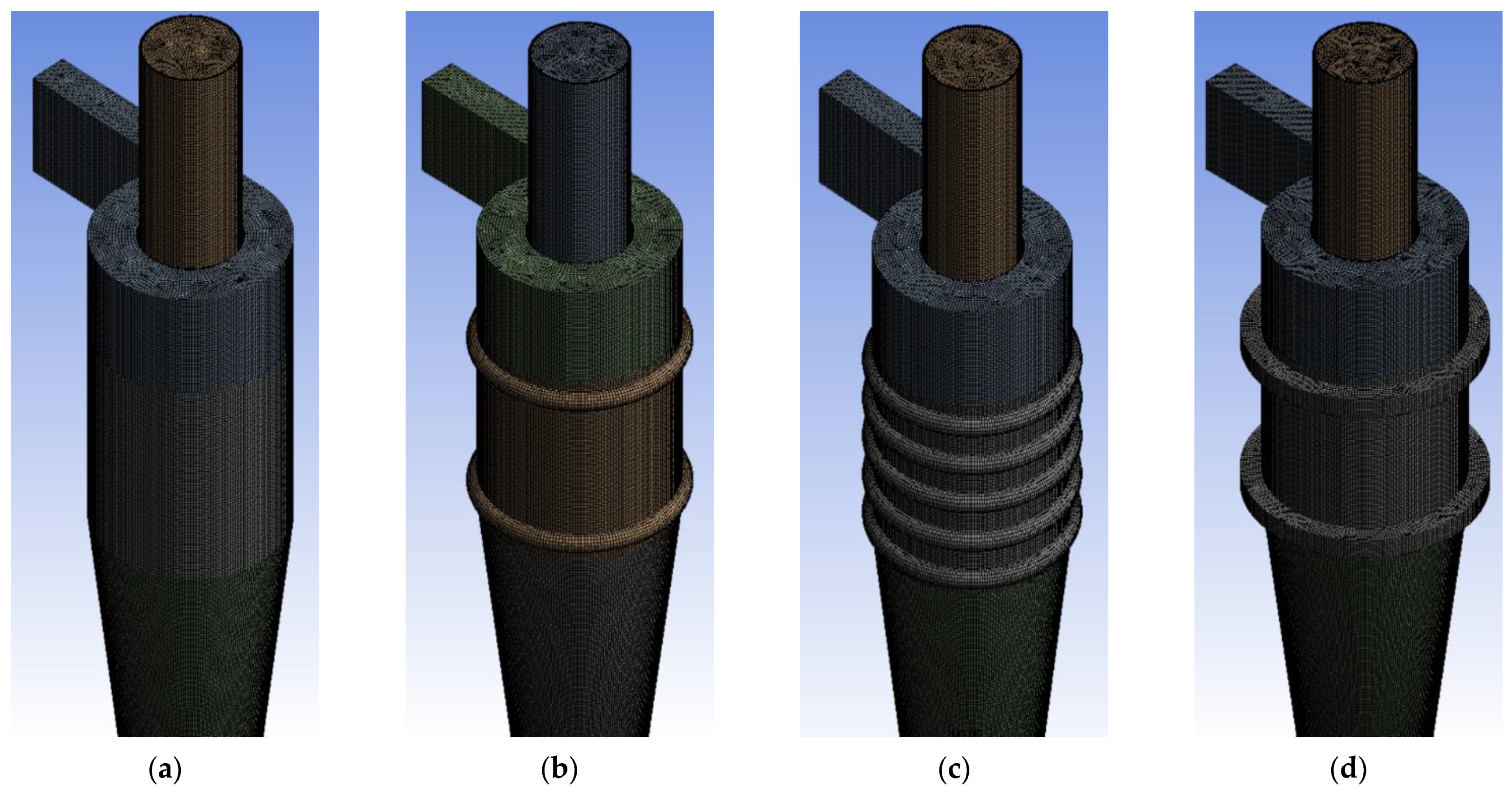
The computational domain was divided into four zones to generate an unstructured hexahedral mesh in each section using the meshing tool from ANSYS Workbench. The hexahedral mesh was generated using the Multizone method; furthermore, a refinement was applied using the local “Inflation” control to be able to predict the boundary layer adequately in the geometrical models in the zones where it is necessary to analyze flow conditions, such as the inlet, the bottom of the conic section and the vortex finder. Figure 2 illustrates the mesh for each of the models.

Various parameters allow for determining the quality of the mesh; the Aspect Ratio (AR) indicates the proportion between the dimensions of the elements, Skewness (S) determinates the mesh quality through its obliqueness, measured in a scale from 0 to 1, where 0 indicates a good quality mesh also the Orthogonal Quality (OQ) is evaluated on a scale from 0 to 1, being 1 is for an appropriate mesh.

Table 2. Mesh quality parameters of cyclone models A, B, C and D.

Mesh	Model A			Model B			Model C			Model D
	AR	OQ	S	AR	OQ	S	AR	OQ	S	AR	OQ	S
Coarse	21.1	1	0.70	61.61	1	0.93	68.51	1	0.93	23.37	1	0.70
Medium	19.66	0.99	0.86	66.81	1	0.94	70.70	1	0.93	23.02	1	0.81
Fine	18.36	1	0.70	71.09	1	0.94	76.71	1	0.94	22.15	1	0.74

* AR is the aspect ratio, OQ is the orthogonal quality and S is the skewness.

shows all the information on the mesh quality parameters for each cyclone model.

4.5. Mesh Convergence Study

The mesh convergence study was done for all the cyclone models. The pressure drop is the comparison parameter calculated in three different grids for each geometry.

Table 3. Mesh independence study for cyclone models.

Mesh	Model A		Model B		Model C		Model D
	Elements	Pressure Drop (Pa)	Elements	Pressure Drop (Pa)	Elements	Pressure Drop (Pa)	Elements	Pressure Drop (Pa)
Coarse	1,020,400	811.63	1,004,665	785.34	1,080,617	764.26	977,769	758.23
Medium	1,225,217	817.81	1,220,779	791.93	1,218,783	774.70	1,224,120	766.59
Fine	1,488,747	823.92	1,445,118	797.95	1,470,052	782.65	1,479,022	774.93
a Percentage change		0.76%		0.84%		1.37%		1.10%
b Percentage change		0.75%		0.76%		1.03%		1.09%

^a Percentage change between the coarse and medium mesh values for pressure drop. ^b Percentage change between the medium and fine mesh values for pressure drop.

shows the number of elements and pressure drop in each mesh implemented.

Note that the percentage change between pressure drop of the coarse and medium meshes, as well as the medium and fine, do not exceed 5%. Therefore, the medium mesh is suitable to solve the calculations in this paper. Also,

Table 4. Area-weighted average $y^{+}$ value obtained for each cyclone model.

Model	${\mathit{y}}^{+}$
A	22.48
B	28.80
C	29.09
D	20.99

shows the area-weighted average $y^{+}$ to highlight the grid refinement near the wall.

In this study, we used RANS equations with wall functions, a value of $y^{+}<30$, indicates that at least 1 point is into the viscous sublayer, which is adequate to model turbulence near the wall, keeping in mind that RANS is not concerned with individual eddy behavior, therefore is not necessary that RANS node spacing be less or equal to the Kolmogorov eddies.

4.6. Computational Conditions

In this study, we used three boundary conditions for the computational model. “Velocity Inlet” condition was used in the cyclone inlet, while the boundary condition “Outflow” was used for the two exits. It is worth mentioning that the flow enters the cyclone with a velocity of 16.1 m/s, the cyclone volume flow rate is 0.135 ${\mathrm{m}}^3/\mathrm{s}$, the fluid temperature is 23 °C, and its static pressure is 1 atm.

Table 5. Boundary conditions.

Section	Boundary Conditions
	Category	DPM
Inlet	Velocity Inlet	Reflect
Vortex finder outlet	Outflow	Escape
Cone bottom	Outflow	Trap

and

Table 6. Properties of the continuous and dispersed phase.

Continuous Phase		Dispersed Phase
Material	Air	Material	Anthracite
Density	1.225 (kg/m3)	Density	2700 (kg/m3)
Dynamic viscosity	1.87 × 10−5 (kg/ms)	Particle size	0.5–7 μm
Reynolds number	2.8 × 105	Diameter distribution	Uniform (10 inyections)

show the boundary conditions in different cyclone zones and the properties of the continuous and disperse phases.

Table 7. Numerical scheme.

Discretization Schemes	Scheme
Pressure–velocity coupling	Coupled
Pressure	Second order upwind
Momentum	Second order upwind
Turbulent kinetic energy	Second order upwind
Turbulent dissipation rate	Second order upwind
Reynolds stress	Second order upwind

shows the discretization schemes for the different flow field variables.

4.7. Simulation Validation

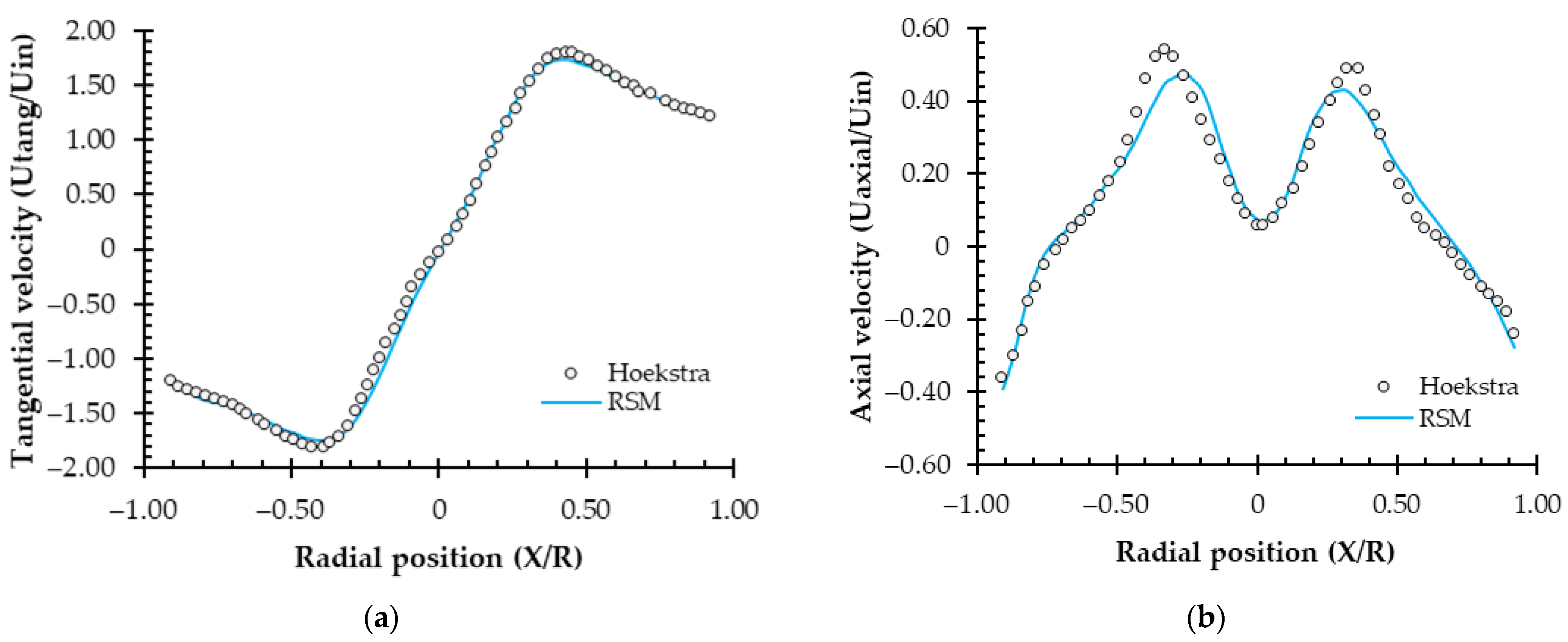
Before continuing with the numeric analysis, it needs to perform numerical results validation against the experimental data for the continuous and discrete phases. Literature includes publications [11,14] that highlight the use of the results obtained by Hoekstra [22] as an experimental model to validate his methodology. Hoekstra ran a series of experiments in the high-efficiency Stairmand cyclone [36] and studied in detail velocity scalar components at various cyclone axial stations using the LDA technique (Laser Doppler Anemometry) [14]. To validate our numeric model, compare pressure drop, separation efficiency, axial and tangential velocity profiles in an axial section located at 0.75 mm from the cyclone roof with the experimental data published by Hoekstra [22].

Figure 3 shows the comparison between the axial and tangential velocity profiles obtained through numerical simulation against published data by [22]. Profile values were obtained using a velocity inlet equal to 16.1 m/s at an axial section located at 217.5 mm (0.75D) from the roof of the cyclone. Comparing the percentage error between the axial and tangential velocity profiles obtained in the numerical study with those published by Hoekstra are from 0.51% to 4.41%, respectively.

Likewise, for validation of the separation efficiency, we use 20 m/s as a velocity inlet like in the Hoeskra study.

Table 8. Validation of pressure drop and separation efficiency parameters.

Model	Pressure Drop (Pa)	Separation Efficiency
Hoekstra	783	63.77%
Numerical simulation	817.81	65.46%
Percentage error	4.45%	2.65%

contains all the details of the validation.

Taking into account the complexity of the turbulent flow in the cyclones, along with the values corresponding to the percentage error obtained previously, it was deemed that the theoretical data and those obtained through computational simulation are in very good agreement.

5. Analysis of the Numerical Results

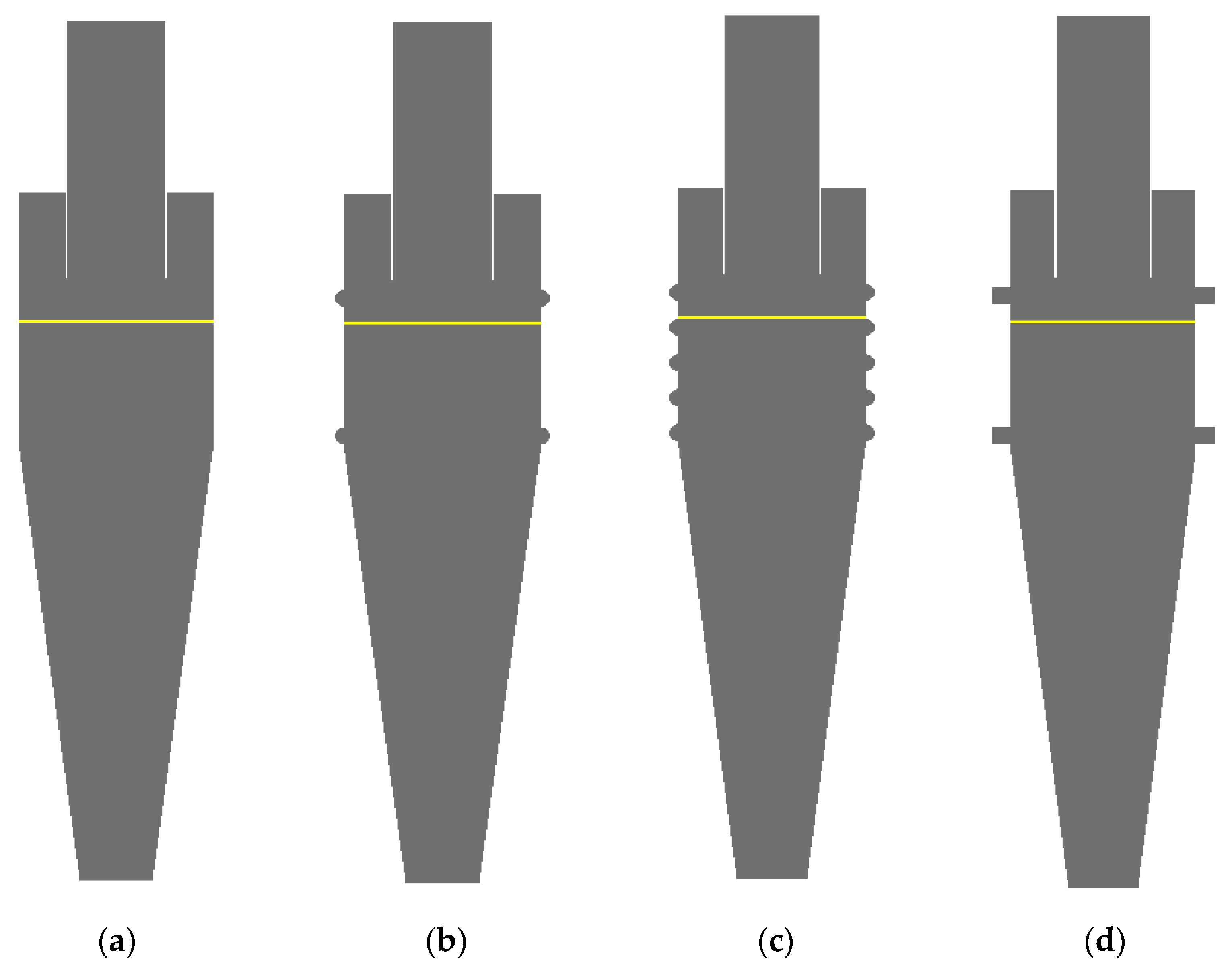
This section shows the performance parameters of the three cyclone separators whose designs incorporate flow control techniques. To this effect, the results of the test models were compared to the standard high-efficiency cyclone. The comparison of the performance parameters between models A, B, C, and D was competed using contour plots and velocity profiles, obtained through a middle plane and a 217.5 mm axial station, as shown in Figure 4.

5.1. Velocity Field

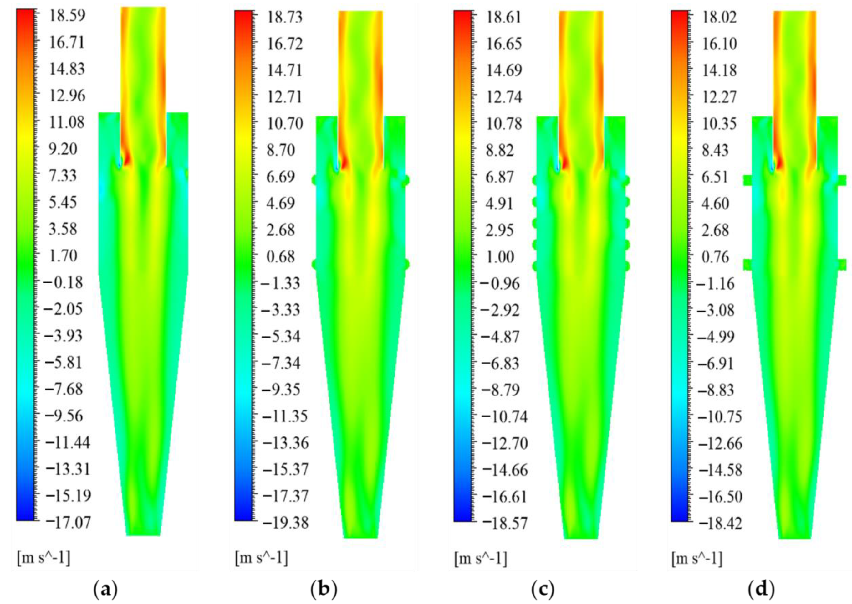
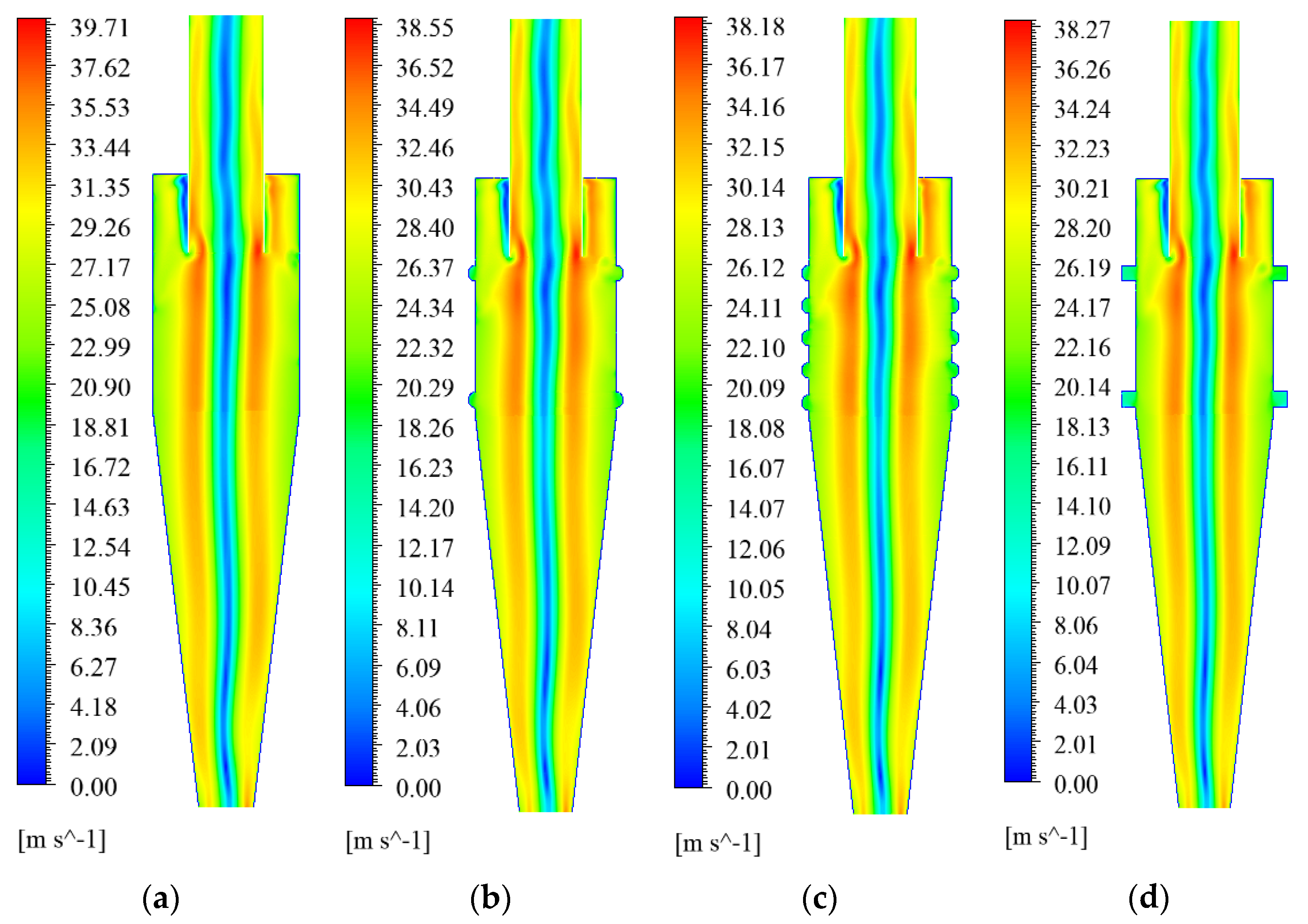
Once the fluid particles are separated by centrifugal force, the axial velocity has an important role since it is primarily responsible for transporting the particulate matter towards the bottom of the cyclone [14,42]. In addition to this, this velocity component is responsible for the direction of both flow currents inside the cyclone [11]. Figure 5 shows the axial velocity contour plots for models A, B, C, and D at the middle plane. Starting from these contour plots, the effect of the double vortex can be seen in the flow of the cyclone, formed by an initial spiral in a descending direction that forms close to the walls of the cyclone, which transports the particles toward its bottom, along with a second spiral in an upward direction in the central region whose purpose is to extract the gas flow through the vortex finder. It is noted that the axial velocity contours for the four models are qualitatively very similar; however, there are quantitative differences between the proposed models and the reference one (Model A); there is the higher axial velocity in models B and C, while in the model D, the axial velocity contours are very similar to the reference model.

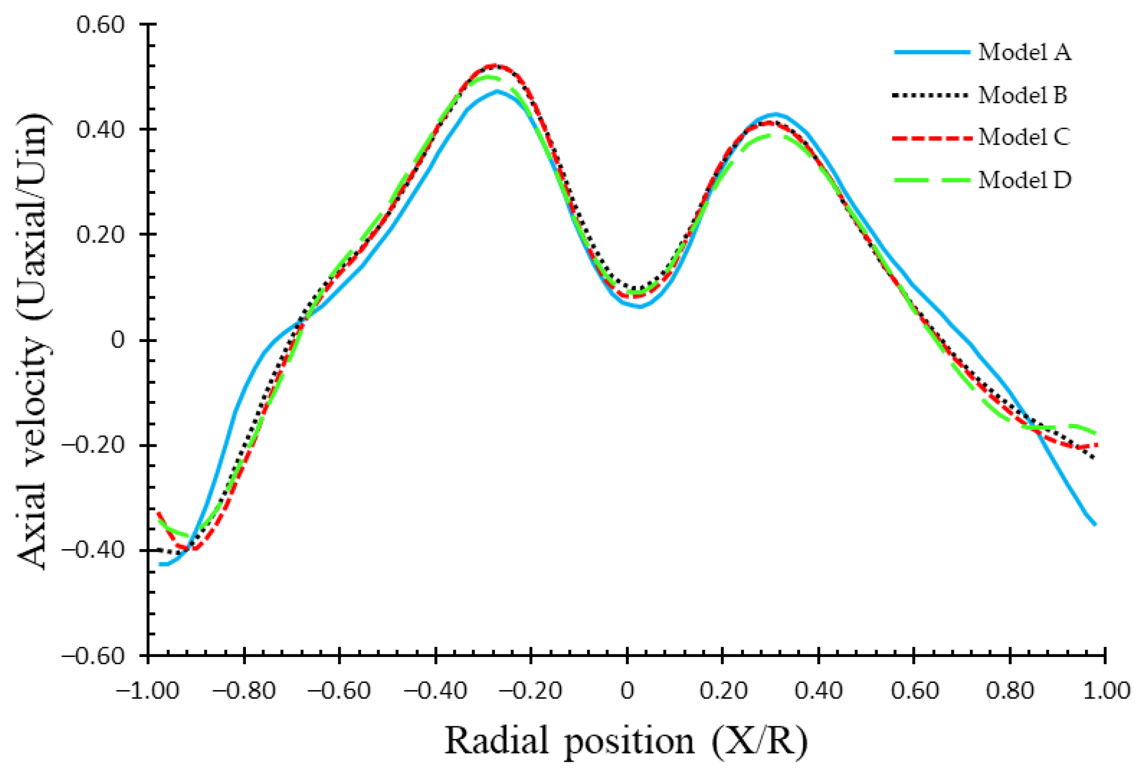
On the other hand, Figure 6 illustrates the axial velocity profiles for the four cyclone models. It shows that the axial velocity profiles of the models are similar in the magnitude of their values as well as their shape (an inverse W). However, it is possible to see an increase in axial velocity in the central region of the profiles of models B, C, and D, as well as a slight decrease in its fall as a result of the increase in kinetic energy that is the result of the passing of flow in the cavities of the cylindrical section of the cyclone. In addition to this, through the axial velocity profiles, the effects of a double vortex in the flow of the cyclone mentioned previously can be seen, because near the wall of the cyclone the values of the axial velocity are negative, thus demonstrating that the direction of the first spiral is descending. Additionally, in the direction of the central region of the cyclone, there is a point where the velocity is zero, indicating the change of direction between both spirals. Finally, in the central region of the cyclone are positive values which confirm that the direction of the second spiral is ascending towards the vortex finder. Apart from that, Figure 6 shows the asymmetry present in each of the profiles. This asymmetric factor is due in part to the spiral flow in the interior of the cyclone and its geometry since the tangential shape inlet section does not allow for its design to be symmetric. In addition, this could be due to instability in the ascending vortex. However, it is worth mentioning that in studies such as [10,41,43] this asymmetric condition is seen in the axial velocity profiles.

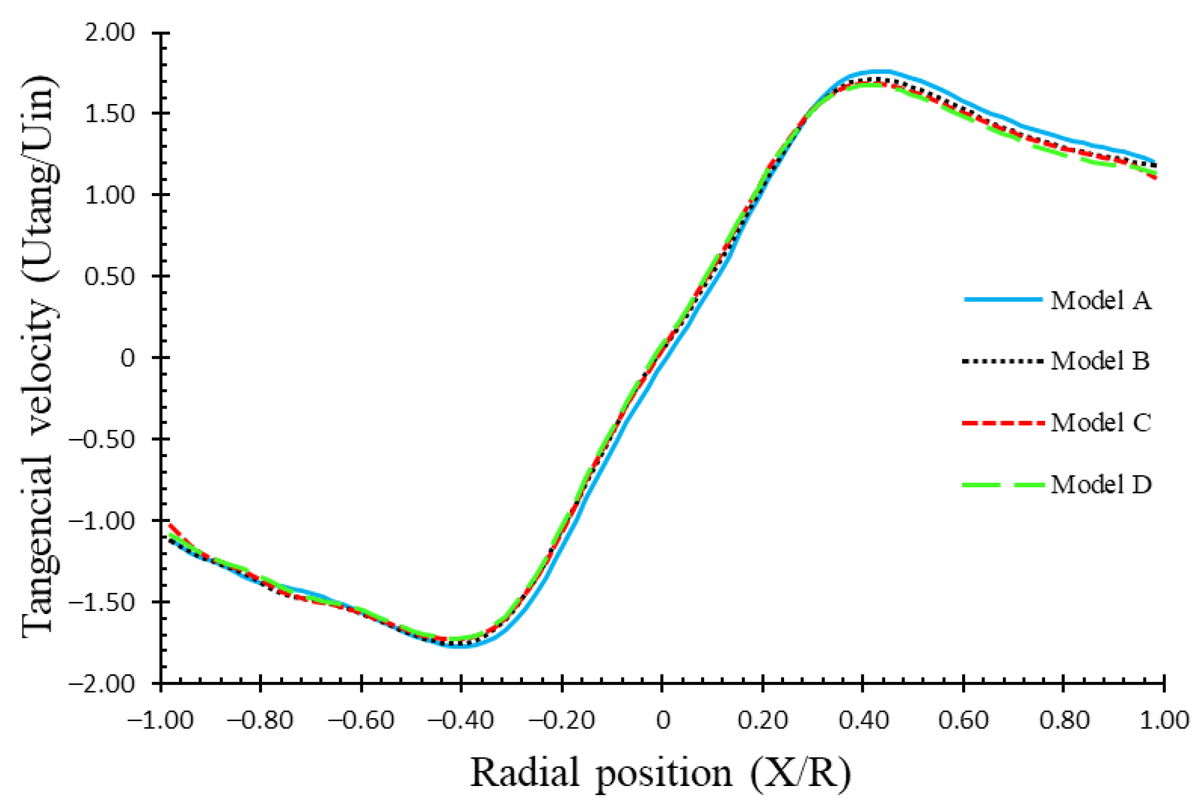
Tangential velocity is the most important parameter regarding flow velocity because it has a great impact on the separation efficiency since it determines the magnitude of the centrifugal force produced in the cyclone [11,22]. Figure 7 illustrates the tangential velocity profiles for all the cyclone models in a 217.5 mm axial station. According to the profiles, it is seen that this model, a Rankine vortex, which is made of an internal forced vortex with a tendency to rotate like a solid, where tangential velocity increases radially from the central axis of the cyclone, as well from a free external vortex, where tangential velocity values decrease as the radial distance increases [10,22]. Besides that, when the values and the shape of the profiles are analyzed between the models, it can be concluded that the flow in cyclones B, C, and D are not affected by the cavities in its cylindrical section, since its velocity profile is similar to model A. However, when the profiles are observed in detail, a decrease in the maximum value of the tangential velocity of cyclones B, C, and D can be seen, thus demonstrating a reduction in the intensity of the swirl in these models regarding Model A, as a result of the flow control technique used.

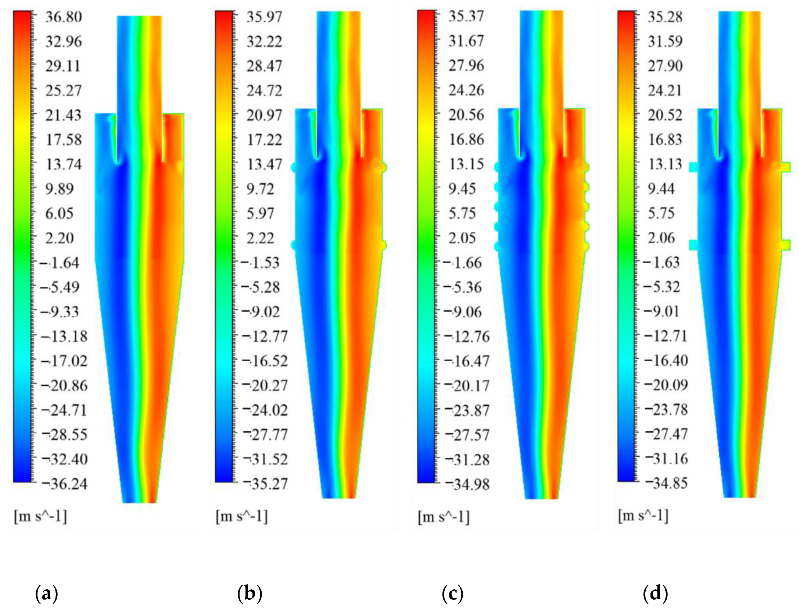
Figure 8 shows the contour plots corresponding to the tangential velocity of the four cyclone separator models at the middle plane. The aforementioned reduction in the turbulent intensity can be verified through the values in the spectrums of the tangential velocity contour plots, as well as the values in Table 8, which has the maximum values of each of the spectrums along with its variation percentage. When the tangential velocity contours and the percentage error in Table 8 for model A are compared against models B, C, and D, a reduction in the tangential velocity values is seen, thus reflecting the reduction of swirl intensity as a result of the passive flow control technique used in the cylindrical section of the models.

Figure 9 shows the contour plots corresponding to the magnitude of the velocity of cyclone models A, B, C, and D at the middle plane, respectively. Just as a decrease in the values of the spectrum in the tangential velocity contour plots of the cyclones with cavities in their cylindrical section was previously demonstrated, when the percentage change of the velocity values is seen in

Table 9. Values and percentage change of mean velocity and tangential velocity of cyclone models A, B, C and D.

Model	A	B	C	D
Tangential velocity (m/s)	36.8	35.97	35.37	35.28
Velocity (m/s)	39.71	38.55	38.18	38.27
aPercentage change	–	−2.26%	−3.89%	−4.13%
bPercentage change	–	−2.92%	−3.85%	−3.63%

^a Percentage change of maximum tangential velocity value relative to Stairmand high-efficiency cyclone. ^b Percentage change of maximum velocity value relative to Stairmand high-efficiency cyclone.

, and the spectrum of the velocity outline between the cyclone models is compared, a reduction in the magnitude of the velocity values of models B, C, and D is seen, due to the geometric modifications made.

5.2. Pressure Drop

The pressure drop of the cyclone is the difference between the inlet and outlet average static pressure values and is directly related to the energy needed to operate the cyclone [9,10].

Table 10. Values and percent change of pressure drop for cyclone models A, B, C, and D.

Model	Pressure Drop (Pa)	a Percentage Difference in Pressure Drop
A	1293.35	–
B	1243.40	−3.86%
C	1222.30	−5.49%
D	1215.67	−6.01%

^a Percentage change in pressure drop relative to Stairmand high-efficiency cyclone (Model A).

contains the pressure drop of all the models simulated under the same operating conditions model A (Stairmand) showed a higher pressure drop and, models B, C, and D, shown a decrease in their pressure drop as a result of the cavities in its cylindrical sections, where model D stood out with a reduction of 6.01% when compared to a standard cyclone. The observed pressure drop can be due to recirculating effects inside of the cavities as is exposed for a channel flow in [29].

Figure 10 illustrates the static pressure contour plots of the four cyclone models at the middle plane. According to these contour plots, the distribution of pressure in the axial direction does not show great variations compared to the radial direction that shows significant variations due to the pressure gradient that results between the walls of the cyclone and its axis [11,22]. Additionally, the pressure contour plots for each of the models show a maximum value on the cyclone wall, a value that decreases radially towards its center, thus illustrating the high- and low-pressure areas that make up the pressure gradient that occur as a result of the rotation of the flow.

5.3. Separation Efficiency

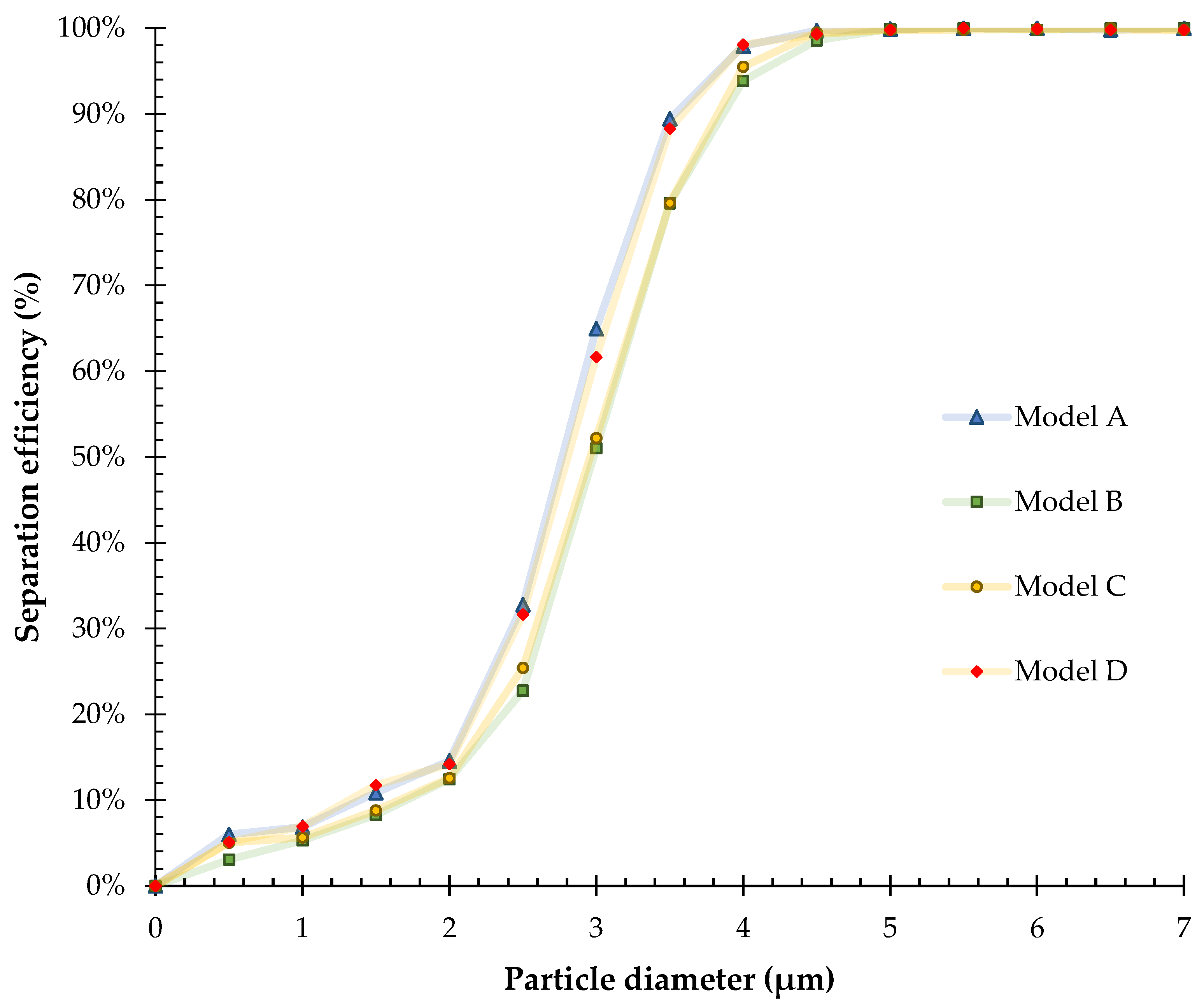
The separation efficiency in a cyclone is the relationship between the number of particles captured with regards to the number of particles that enter by its inlet section [9,14]. This collection capacity is denoted in terms of its global efficiency or the cut-off diameter (d₅₀), the latter being the particle diameter whose separation efficiency is 50% [10]. In this paper, the separation efficiency presented by each of the cyclone models is considered globally, as well as fractionally, by using a graph called grade efficiency curve, which relates the separation efficiency of each model with the diameter of the particle.

Figure 11 shows the grade efficiency curves of the four cyclone models. The cut-off diameter for each model is 2.76 μm, 2.98 μm, 2.96 μm, and 2.81 μm, respectively. In comparison with the Stairmand high-efficiency model (Model A), all the other models show an increase of the cut-off diameter, being the model D, the one that increases the less, which coincidentally is the model that generated the higher pressure drop reduction, as was already shown in Table 10.

Additionally,

Table 11. Values and percent change in separation efficiency for cyclone models A, B, C, and D.

Model	Separation Efficiency	a Percentage Change in Separation Efficiency
A	65.46%	–
B	62.61%	−4.35
C	62.96%	−3.81
D	65.18%	−0.42

^a Percentage change in separation efficiency relative to Stairmand high-efficiency cyclone (Model A).

shows the values referring to the overall separation efficiency presented by all the cyclone models, along with their percentage change concerning the standard model (Model A). Table 11 shows that the application of circular cavities as a passive flow control technique does not favor the particle collection in the cyclones. The models B and C efficiency of separation decrease 4.35% and 3.81%, respectively, regarding model A. The separation efficiency values of models A and D differ only by 0.42% and, additionally model D presented the highest reduction in pressure drop too, therefore could be considered that this cyclone exhibits the same or almost the same particle collection capacity as Model A, having the advantage that its pressure drop is way less.

6. Conclusions

The cylindrical section of the high-efficiency Stairmand model was modified, applying cavities as a passive flow control technique to characterize a new cyclone separator model using computational fluid dynamics. Numeric simulations were performed using RANS equations with an RSM turbulence model (including wall functions) to solve the continuous phase (air) and a Lagrangian tracking to solve solid particle movement, considering one-way coupling. The simulation results showed that the implementation of geometric disturbances in the cavity shape of the cyclones as passive flow control favored the reduction of pressure drop since all modified models showed a reduction in their pressure drop compared to the standard model. Furthermore, for all cases with circular cavities, the separation efficiency had a slight decrement with a lower pressure drop concerning the standard model. These findings reinforce the idea that using passive control techniques can help to improve cyclone performance; the latter is important because it opens a new field of study on cyclone separators that have not been used before to the author’s best knowledge. For future studies, it is recommended to evaluate the use and performance of passive flow techniques in new designs of cyclone separators with two-way coupling between continuous and disperse phases, including thermal effects, to consider new alternatives that allow for the improvement of the operation of this equipment.

References

- Contaminación atmosférica. Boletín Calidad del Aire, IDEAM. 2020. Available online: http://www.ideam.gov.co/web/contaminacion-y-calidad-ambiental/contaminacion-atmosferica (accessed on 3 January 2021).
- Arciniegas Suárez, C.A. Diagnóstico y control de material particulado: Partículas suspendidas totales y fracción respirable PM 10. Luna Azul 2012, 34, 195–213. [Google Scholar]
- Cataño, S.J.; Escobar, D.M.; Isaza, D.R. Problemática de la contaminación del aire en Colombia y estrategias de solución para la calidad del Aire en Medellín, Área Metropolitana del Valle de Aburrá (Antioquia). Rev. Ambient. Éolo 2019, 18, 1–14. [Google Scholar]
- López, M.; Vega, A. Estrategias de Mejoramiento de la Calidad del Aire en Ciudades con Problemas de Contaminación; Monografía de Especialización; Universidad de Antioquia: Antioquia, Colombia, 2019. [Google Scholar]
- Meléndez Gélvez, I.; Quijano Vargas, M.J.; Quijano Parra, A. Actividad mutagénica inducida por hidrocarburos aromáticos policíclicos en muestras de PM2.5 en un sector residencial de villa del rosario-Norte de Santander, Colombia. Rev. Int. Contam. Ambie. 2016, 32, 435–444. [Google Scholar] [CrossRef] [Green Version]
- García Ávila, P.A.; Rojas, N.Y. Análisis del origen de PM10 y PM2.5 en Bogotá gráficos polares. Rev. Mutis. 2016, 6, 47–58. [Google Scholar] [CrossRef]
- Muñoz, A.; Palacio, C.; Paz, J. Efectos de la Contaminación Atmosférica Sobre la Salud en Adultos que Laboran a Diferentes Niveles de Exposición. Master’s Thesis, Universidad de Antioquia, Antioquia, Colombia, 2006. [Google Scholar]
- Cortes, S. Material Particulado en el Aire y su Correlación con la Función Pulmonar en Personas que Realizan Actividad Física en la Cicloruta en la Localidad Kennedy en Bogotá: Estudio Descriptivo Transversal. Master’s Thesis, Universidad Nacional de Colombia, Bogotá, Colombia, 2018. [Google Scholar]
- Bahamondes, J.L. Diseño y Construcción de un Separador Ciclónico para la Industria Naval. Bachelor’s Thesis, Universidad Austral de Chile, Valdivia, Chile, 2008. [Google Scholar]
- Brar, L.S.; Sharma, R.P.; Elsayed, K. The effect of the cyclone length on the performance of Stairmand high-efficiency cyclone. Powder Technol. 2015, 286, 668–677. [Google Scholar] [CrossRef]
- Hamdy, O.; Bassily, M.A.; El-batsh, H.M.; Mekhail, T.A. Numerical study of the effect of changing the cyclone cone length on the gas flow field. Appl. Math. Model. 2017, 46, 81–97. [Google Scholar] [CrossRef]
- Wasilewski, M.; Singh, L.; Ligus, G. Experimental and numerical investigation on the performance of square cyclones with different vortex finder configurations. Sep. Purif. Technol. 2020, 239, 10–24. [Google Scholar] [CrossRef]
- González, W.; Medina, S. Diseño e Implementación de un Equipo Separador de Partículas Sólidas (ciclón) en la Industria del Caucho. Bachelor’s Thesis, Universidad Central del Ecuador, Quito, Ecuador, 2018. [Google Scholar]
- Brar, L.S.; Sharma, R.P.; Dwivedi, R. Effect of vortex finder diameter on flow field and collection efficiency of cyclone separators. Part. Sci. Technol. 2015, 33, 34–40. [Google Scholar] [CrossRef]
- Wang, B.; Xu, D.L.; Chu, K.W.; Yu, A.B. Numerical study of gas–solid flow in a cyclone separator. Appl. Math. Model. 2006, 30, 1326–1342. [Google Scholar] [CrossRef] [Green Version]
- Chuah, T.G.; Gimbun, J.; Choong, T.S.Y. A CFD study of the effect of cone dimensions on sampling aerocyclones performance and hydrodynamics. Powder Technol. 2006, 162, 126–132. [Google Scholar] [CrossRef]
- Hoffmann, A.; Groot, M.; Peng, W.; Kater, J.; Dries, H. Advantages and risks in increasing cyclone separator length. AIChE J. 2001, 47, 2452–2460. [Google Scholar] [CrossRef]
- Zhao, B.; Shen, H.; Kang, Y. Development of a symmetrical spiral inlet to improve cyclone separator performance. Powder Technol. 2004, 145, 47–50. [Google Scholar] [CrossRef]
- Elsayed, K.; Lacor, C. The effect of cyclone inlet dimensions on the flow pattern and performance. Appl. Math. Model. 2011, 35, 1952–1968. [Google Scholar] [CrossRef] [Green Version]
- Elsayed, K.; Lacor, C. Numerical modeling of the flow field and performance in cyclones of different cone-tip diameters. Comput. Fluids 2011, 51, 48–59. [Google Scholar] [CrossRef]
- Xiang, R.B.; Park, S.H.; Lee, K.W. Effects of cone dimension on cyclone performance. Aerosol Sci. 2001, 32, 549–561. [Google Scholar] [CrossRef]
- Hoekstra, A.J. Gas Flow Field and Collection Efficiency of Cyclone Separators. Ph.D. Thesis, Technical University Delft, Delft, The Netherlands, 2000. [Google Scholar]
- El-Batsh, H.M. Improving cyclone performance by proper selection of the exit pipe. Appl. Math. Model. 2013, 37, 5286–5303. [Google Scholar] [CrossRef]
- Xiang, R.B.; Lee, K.W. Effects of exit tube diameter on the flow field in cyclones. Part. Sci. Technol. 2008, 26, 476–481. [Google Scholar] [CrossRef]
- Leonardi, S.; Orlandi, P.; Smalley, R.J.; Djenidi, L.; Antonia, R.A. Direct numerical simulations of turbulent channel flow with transverse square bars on one wall. Cambridge Univ. Press 2003, 491, 229–238. [Google Scholar] [CrossRef] [Green Version]
- Yagiz, B.; Kandil, O.; Pehlivanoglu, Y.V. Drag minimization using active and passive flow control techniques. Aerosp. Sci. Technol. 2012, 17, 21–31. [Google Scholar] [CrossRef]
- Camocardi, M.E. Control de Flujo Sobre la Estela Cercana de Perfiles Aerodinámicos Mediante la Implementación de Mini-Flaps Gurney. Ph.D. Thesis, Universidad Nacional de la Plata, La Plata, Argentina, 2012. [Google Scholar]
- Choi, K.-S.; Fujisawa, N. Possibility of drag reduction using d-type roughness. Appl. Sci. Res. 1993, 50, 315–324. [Google Scholar] [CrossRef]
- Pastrán, J.A.R. Investigación Numérica de un Flujo Incompresible Turbulento Cargado con Partículas Sólidas Suspendidas a Través de un Canal con Perturbaciones de Pared Controladas. Ph.D. Thesis, Universidad Nacional de Colombia, Bogotá, Colombia, 2018. [Google Scholar]
- Fiedler, H.E. Flow Control: Control of free turbulent shear flows. In Flow Control Fundamentals and Practices; Gad-el-Hak, M., Pollard, A., Bonnet, J.P., Eds.; Springer: Berlin/Heidelberg, Germany; New York, NY, USA, 1998; pp. 335–429. [Google Scholar]
- Strykowski, P.J.; Forliti, D.J. Flow control applications using countercurrent shear. In Proceedings of the International Symposium on Recent Advances in Experimental Fluid Mechanics, Kampur, India, 18–20 December 2000; pp. 1–16. [Google Scholar]
- Yousefi, K.; Saleh, R. Three-dimensional suction flow control and suction jet length optimization of NACA 0012 wing. HAL Arch. 2017, 50, 1481–1494. [Google Scholar] [CrossRef]
- Gad el Hak, M. Modern developments in flow control. Appl. Mech. Rev. 1996, 49, 365–379. [Google Scholar] [CrossRef]
- Thomaz, C.R., Jr.; Calderón Muñoz, W. Desempeño Aerodinámico de Turbinas Eólicas de Eje Vertical en Función de Temperatura de Superficie de Álabe. Master’s Thesis, Universidad de Chile, San Diego, Chile, 2012. [Google Scholar]
- Hernandez, L.; Aldana, Y.; Bocanegra, W. Estudio y Análisis de Técnicas que Evitan el Desprendimiento de la Capa Límite en un Perfil Aerodinámico a Bajas Velocidades. Bachelor’s Thesis, Universidad de San Buenaventura, Buenaventura, Colombia, 2005. [Google Scholar]
- Stairmand, C.J. The design and performance of cyclone separators. Trans. I Chem. E 1951, 29, 356–383. [Google Scholar]
- Ansys® Fluent Theory Guide 2019R2, Section 4.1.2; ANSYS, Inc.: Canonsburg, PA, USA, 2019.
- Huang, H.; Sun, T.; Zhang, L.D.; Wei, H. Evaluation of a developed SST k-ω turbulence model for the prediction of turbulent slot jet impingement heat transfer. Int. J. Heat Mass Transf. 2019, 139, 700–712. [Google Scholar] [CrossRef]
- Cademartori, C.; Cravero, C.; Marini, M.; Marsano, D. CFD simulation of the slot jet impingement heat transfer process and application to a temperature control system for galvanizing line of metal band. Appl. Sci. 2021, 11, 1149. [Google Scholar] [CrossRef]
- Derksen, J.J.; Van Den Akker, H.E.A. Two way coupled Large-Eddy simulations of the gas-solid flow in cyclone separators. AIChE J. 2008, 54, 872–885. [Google Scholar] [CrossRef]
- Shukla, S.K.; Shukla, P.; Ghosh, P. Evaluation of numerical schemes for dispersed phase modeling of cyclone separators. Eng. Appl. Comput. Fluid Mech. 2014, 5, 235–246. [Google Scholar] [CrossRef] [Green Version]
- Chu, K.W.; Wang, B.D.; Xu, L.; Chen, Y.X.; Yu, A.B. CFD–DEM simulation of the gas–solid flow in a cyclone separator. Chem. Eng. Sci. 2011, 66, 834–847. [Google Scholar] [CrossRef]
- Singh, L.; Elsayed, K. Analysis and optimization of multi-inlet gas cyclones using large eddy simulation and artificial neural network. Powder Technol. 2017, 311, 465–483. [Google Scholar]
Figure 1.
Schematic diagram of cyclone models; (a) Model A (Stairmand cyclone separator), (b) Model B cyclone separator, (c) Model C cyclone separator, (d) Model D cyclone separator.
Figure 2.
Meshing of cyclone models; (a) Model A (Stairmand) cyclone separator, (b) Model B cyclone separator, (c) Model C cyclone separator, (d) Model D cyclone separator.
Figure 3.
Comparison of velocity profiles between numerical simulation and results of Hoekstra; (a) Tangential velocity profiles, (b) Axial velocity profiles.
Figure 4.
Axial stations and middle planes of cyclones; (a) Stairmand cyclone separator, (b) Model B cyclone separator, (c) Model C cyclone separator, (d) Model D cyclone separator.
Figure 5.
Contour plots of axial velocity of cyclone models; (a) Stairmand cyclone separator, (b) Model B cyclone separator, (c) Model C cyclone separator, (d) Model D cyclone separator.
Figure 6.
Axial velocity profiles of cyclone models A, B, C y D.
Figure 7.
Tangential velocity profiles of cyclone models A, B, C y D.
Figure 8.
Contour plots of tangential velocity of cyclone models; (a) Model A (Stairmand cyclone separator), (b) Model B cyclone separator, (c) Model C cyclone separator, (d) Model D cyclone separator.
Figure 9.
Contour plots of velocity magnitude of cyclone models; (a) Model A (Stairmand cyclone separator), (b) Model B cyclone separator, (c) Model C cyclone separator, (d) Model D cyclone separator.
Figure 10.
Contour plots of static pressure of cyclone models; (a) Model A (Stairmand cyclone separator), (b) Model B cyclone separator, (c) Model C cyclone separator, (d) Model D cyclone separator.
Figure 11.
Grade efficiency curves of cyclone models A, B, C y D.