Numerical and Experimental Analysis of Flow and Pulsation in Hump Section of Siphon Outlet Conduit of Axial Flow Pump Device

Abstract

In order to study the variation law of the flow field and pressure fluctuation in the hump section of the siphon outlet conduit, the flow field characteristics and frequency spectrum characteristics of the flow field were analyzed by combining a physical model test and numerical simulation under the conditions of the interaction between the axial flow pump and siphon outlet conduit, and the influence of the residual circulation at the outlet of the guide vane on the siphon outlet flow was investigated. Based on the influence of the flow field and hydraulic loss in the conduit, the equivalent surface method based on the Q criterion was used to analyze the vortex structure in the siphon outlet conduit and to analyze the internal vortex state. The results showed that with the increase of the flow rate, the intensity of the vortices in the cross-section of the hump section of the siphon outlet conduit decreased gradually, the average velocity circulation decreased gradually and the axial velocity distribution uniformity increased and tended to be stable; water flow stratification existed under three characteristic conditions with no circulation, and the hydraulic loss was greater with the circulation flow while it had a circulation under the small flow condition. Under the low flow rate conditions, the hydraulic loss was 6.6 times higher under the condition of circulation than without. Under a high flow condition, it was 1.3 times. Under the condition of a small flow rate, the vortex structure was distributed centrally at the inlet of the flow conduit, and under the other two characteristic conditions, the vortex structure mostly appeared as a strip; the pressure fluctuation in the hump section had obvious periodicity, and with the increase of the flow rate, the maximum pressure fluctuation amplitude in the hump section decreased gradually; with the decrease of the rotational speed, the pressure amplitude at the same measuring point in the hump section decreased gradually and at the optimum condition. Under the following conditions, the mean value of the pressure amplitude at the top of the hump section was reduced by 69.63%, and the mean value of the pressure amplitude at the bottom of the hump section was reduced by 63.5%. Under all the calculation conditions, the main frequency of pulsation at each measuring point of the hump section was twice the frequency of the rotation.

1. Introduction

The South-to-North Water Transfer Project is one of the most important water conservancy projects in China in the 21st century. It is the largest inter-basin water transfer project in the world. Its total investment is estimated to exceed US $76 billion, involving 438 million people and over 40,000,000,000 m³ of water. It mainly solves the problems of water shortage and distribution in Northern China [1,2]. A total of 35 pumping stations have been constructed in Phase I of the east route of the South-to-North Water Transfer Project. Among the 21 new pumping stations, the number of large vertical axial flow pumping units accounts for more than 66%, which is the main structural type of pumping unit used in the project. The siphon outlet conduit is one of the common outlet structures for large-scale low-head pump units. It is suitable for situations where the water level of the outlet pool varies little. Its cut-off mode has the advantages of simplicity, reliability and economy.

However, the siphon outlet conduit has the disadvantages of a complex shape and inconvenient construction. The advantages and disadvantages of the siphon outlet conduit are comprehensively analyzed. In the first stage of the east route of the South-to-North Water Transfer Project of China, the siphon outlet conduit had advantages and disadvantages. Seven of the 14 new vertical pumping stations in the project employ siphon outlet conduits accounted for 50%, such as Liu Laojian No.2 station, Siyang pump station, Suining No.2 station and Denglou pump station in Jiangsu Province. The internal flow characteristics of the outlet conduit will not only affect the safe and stable operation of the pump unit but also affect the hydraulic efficiency of the pump unit. The hydraulic loss of the outlet conduit accounts for a large proportion of the factors affecting the hydraulic efficiency. The internal flow of the siphon outlet conduit is complicated due to the influence of the axial flow pump. Domestic and international scholars have carried out relevant research work on the siphon outlet conduit. Zhou [3] used the SST k-ω turbulence model and the Zwart cavitation model closed multiphase flow control equations to numerically analyze the cavitation characteristics inside the siphon outflow conduit. Zhang [4] analyzed the influencing factors of hydraulic loss in the condition of a gas–liquid two-phase flow in the siphon flow conduit by the physical model test method and measured the bubble velocity, pressure drop and gas volume fraction in the siphon flow conduit under different operating conditions. Liu [5] used numerical simulations to analyze the transient flow characteristics inside the siphon outlet conduit of a vertical axial flow pumping device during shutdown conditions. Yang [6] carried out full flow conduit numerical calculations for a siphon axial flow pump unit by the CFD method and quantitatively analyzed the influence of the residual circulation at the guide vane outlet and flow rate on the hydraulic loss of the siphon outlet conduit. Wang [7] used the Euler multiphase flow model and RNG k-ε turbulence model to simulate a gas–liquid two-phase flow in the siphon process of the siphon outlet conduit of a pump station. Lu [8,9] modified the geometrical dimensions of the siphon outlet conduits of the pumping stations one by one, observed the changes of the flow patterns inside the conduits by the CFD method and gradually optimized the flow path profile and carried out the comparison of the siphon and straight pipe outlet conduits used in vertical pumps. Liu [10] applied aerodynamic principles to develop a mathematical model for the calculation of the maximum start-up head of a siphon outlet conduit at a pumping station and compared it with the experiments. Shomayramov [11] investigated the effect of the siphon section length and cross-sectional area on the efficiency of the pumping unit through physical model tests and studied the siphon outlet conduit vacuum breaker. Cognet [12] studied the way the siphon conduit works performed experimental measurements during the transient flow in the siphon and measured the fluid velocity distribution using the PIV technique. K. Babaeyan-Koopaei [13] studied the optimization of the geometric parameters of the siphon conduit of the hydraulic performance through the physical model test.

Currently, scholars at home and abroad have focused on the optimization of the overall hydraulic performance of the siphon outlet conduit and the dynamic process of siphon formation, but little research has been done on the internal flow characteristics of the hump section of the siphon outlet conduit. Therefore, the study of the hydraulic properties of the hump section is of reference value for the optimization of the siphon outlet conduit and the safe and stable operation of the siphon outlet conduit pumping unit. In this paper, the flow field and pulsation characteristics in the hump section of the siphon discharge conduit are analyzed by physical model tests combined with numerical simulations for the vertical axial flow pump unit as a whole.

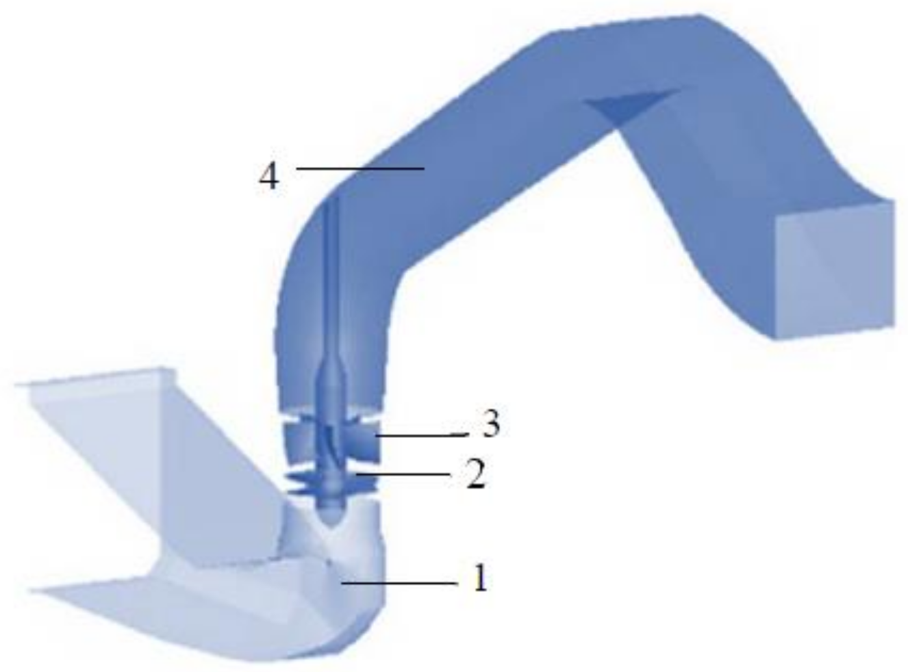
2. Study Object

To study the flow and pulsation characteristics in the hump section of the siphon outlet conduit, this paper takes the full flow path of a vertical axial flow pump device as the research object. The vertical axial flow pump device consists of four flow passages: elbow inlet conduit, impeller, guide vane body and siphon outlet conduit. The three-dimensional model of the vertical axial flow pump device is shown in Figure 1. The main parameters of the impeller and guide vane are shown in

Table 1. Main parameters of the impeller and guide vane.

Impeller diameter/mm	120
Hub Ratio	0.40
Number of impeller blades	4
Blade placement angle	0°
Average tip clearance/mm	0.1
Speed/r·min−1	2200
Number of guide vanes	5

. Including the intake extension section, elbow intake conduit, impeller, guide vane body, siphon outlet conduit and outlet extension section, there are six parts.

The siphon outlet conduit is composed of three sections, i.e., upstream section, hump section and downstream section. Figure 2 is a schematic diagram of the siphon outlet conduit geometry. The main control parameters of the siphon outlet conduit: an inclination of the ascending section is 30 degrees, inclination of the descending section is 44°, horizontal projection length of the flow conduit is 7.05D, the height of the flow conduit is 2.94D, the inlet section diameter of the flow conduit is 1.17D, the outlet section height of the flow conduit is 1.33D, an outlet section width of the flow conduit is 1.60D, the hump section height is 0.75D and hump section width is 1.60D, D is the nominal diameter of the impeller and the flow rate in the hump section is 0.897 m/s at the maximum head (flow ratio is 0.5), which is greater than the minimum flow rate formed by the full pipe siphon at 0.595 m/s.

3. Model Test and Method

3.1. Test Bed and Model

The model test of the vertical axial flow pump device was carried out on the Φ 120-mm hydraulic machinery closed cycle test bed (Figure 3) in the key laboratory of Jiangsu Province. The physical model of the vertical axial flow pump device is shown in Figure 4. A CY302 high-precision digital pressure sensor was used for the pressure fluctuation test. The synchronous data acquisition of six pressure sensors was realized by 485 hubs and data acquisition software. Three pressure sensors were, respectively, arranged at the top and bottom of the hump section of the siphon outlet conduit. Measuring points P2 and P5 were located at the center of the top and bottom of the hump section. Measuring point P1 and P3 are symmetrically arranged on both sides of measuring point P2. Measuring point P4 and P6 are symmetrically arranged on both sides of measuring point P5. The distance between the two sides of P5 and the center of P6 was 35% of the top width of the hump. The arrangement of the pressure sensor and the sequence of each measuring point are shown in Figure 5. The actual model of the impeller and guide vane body are shown in Figure 6 and Figure 7. The pressure pulsation test was carried out simultaneously under the conditions of the energy performance test of the vertical axial flow pump device. The energy performance test of the pump device was carried out in accordance with the requirements of the acceptance test specifications for the pump model and pump device model (SL140-2006 [14]). The pressure pulsation values of each measuring point on the hump wall of the siphon outlet conduit at the speed of 2200 r/min were tested. The internal flow pattern of the hump section of the siphon outlet conduit was observed by sticking a red silk line inside. The red silk line had good flow following the property and could better reflect the flow state of the water. During the energy performance test of the pump device, the flow pattern characteristics of the hump section were evaluated by observing the offset direction and angle of the red silk line.

3.2. Test Reliability Verification

In order to verify the reliability of the energy performance test of the vertical axial flow pump device, the flow–head data of the vertical axial flow pump device was collected repeatedly at 2200 r/min by the same test method. The flow ratio R_Q (Equation (1)) was used for the comparisons under each working condition. After the analysis, the data was collected at 2200 r/min. The repeatability of the flow–head curve of the vertical axial flow pump device was very good at r/min (Figure 8). The data collected from the energy performance of the vertical axial flow pump device under the same conditions were very close, which indicates the reliability of the comprehensive test on this test stand.

$$R_Q=Q_i/Q_{BEP}$$

(1)

where Q_i is the flow rate of the pump unit. and Q_BEP is the flow rate of the pump unit under the optimum operating conditions.

3.3. Comprehensive Uncertainty Analysis

Relative uncertainty of the measuring model efficiency under the selected optimum operating conditions was collected 10 times and calculated with random uncertainty. Student t distribution was used according to the International Electrotechnical Commission’s (IEC) standard IEC 60601-2-24 [15].

Standard deviation of the average efficiency:

$$S_{\overline{\eta }}=\sqrt{\sum \frac{{({\eta }_i-\overline{\eta })}^2}{N\left(N-1\right)}}=0.049$$

(2)

where N is the number of measurements, ${\eta }_i$ is the ith efficiency measurement and ${\eta }_i$ is the average efficiency.

Random uncertainty of the test bench efficiency:

$$E_r=\pm \frac{t_{0.95\left(N-1\right)}\times S_{\overline{\eta }}}{\overline{\eta }}\times 100\%=\pm 0.148\%$$

(3)

where $t_{0.95\left(N-1\right)}$ is the t distribution corresponding to a 0.95 confidence rate and (N − 1) degrees of freedom:

$$t_{0.95\left(9\right)}=2.226$$

Due to the application of high-precision measuring instruments and automatic data acquisition and a processing system, the random uncertainty in the measurements is greatly reduced, and the system uncertainty becomes the main part of the uncertainty. Th system uncertainty consists of the head uncertainty, torque–speed uncertainty and flow uncertainty and is calculated as follows:

Head uncertainty:

$$E_{\mathrm{H}}=\sqrt{E_p^2{+E}_d^2}=\pm 0.01\%$$

(4)

where E_p is the static head uncertainty caused by the pressure gauge and differential pressure sensor, E_p = ±0.1%, and E_d is the dynamic head uncertainty. In this model test, the inlet and outlet pressure measuring points were on the inlet and outlet tanks, E_d = 0.

Uncertainty of the torque speed:

$$E_{\mathrm{T}}=\sqrt{E_m^2{+E}_n^2}=\pm 0.141\%$$

(5)

where E_m is the torque uncertainty and equipment ex-factory calibration, E_m= 0.1%, and E_n is the uncertainty of the speed measurements, E_n = 0.1%.

Uncertainty of the flow measurements:

$$E_{\mathrm{Q}}=\pm 0.1\%$$

(6)

Uncertainty of the test bench system:

$$E_{\mathrm{s}}=\sqrt{E_{\mathrm{H}}^2{+E}_{\mathrm{T}}^2+E_{\mathrm{Q}}^2}=\pm 0.173\%$$

(7)

Therefore, the comprehensive uncertainty of the test efficiency is

$$E_{\mathsf{\eta }}=\sqrt{E_{\mathrm{s}}^2{+E}_{\mathrm{r}}^2}=\pm 0.228\%$$

(8)

4. Numerical Method and Verification

4.1. Governing Equations and Turbulence Models

The fluid movement follows the law of mass conservation, momentum conservation and energy conservation. The flow inside the pump can be considered as incompressible three-dimensional viscous turbulence, ignoring the heat transfer and following the basic laws of the conservation of mass and momentum.

Continuity equation [16]:

$$\frac{\partial \rho }{\partial t}+\frac{\partial \left(\rho u_i\right)}{\partial x_i}=0$$

(9)

In this paper, we used the method of classical uncertainty assessment. The continuity equation is expressed as:

$$\frac{\partial \rho }{\partial t}=\frac{\partial u_i}{\partial x_i}=0$$

(10)

Momentum equation [17]:

$$\frac{\partial \left(\rho u_i\right)}{\partial t}+\frac{\partial \left(\rho u_j{u}_i\right)}{\partial x_j}=-\frac{\partial p}{\partial x_i}+\frac{\partial }{\partial x_j}\left[{\mu }_{eff}\left(\frac{\partial u_i}{\partial x_j}+\frac{\partial u_j}{\partial x_i}\right)\right]+F_i$$

(11)

where ρ is the fluid density, u_i and u_j are the components of the fluid velocity along the i and j directions, respectively, and x_i is the coordinate component, t is the time, P is the pressure on the fluid microelement body, μ is the kinematic viscosity coefficient of the fluid, μ_eff is the effective viscosity coefficient and F_i is the volume force component in the i direction.

The RNG k-ε turbulence model was proposed by Yakhot and Orzag [18] in 1986. It is derived from the instantaneous Navier–Stokes equation by using the mathematical method of group recombination. In the RNG k-ε turbulence model, the small-scale motion is systematically removed from the governing equation by reflecting the small-scale effect in the large-scale motion and the modified viscosity term. The RNG k-ε turbulence model can better simulate the flow with a high strain rate and large curvature of the streamline by modifying the turbulent viscosity and considering the rotating and swirling flows in the average flow. At the same time, it can effectively predict the three-dimensional flow characteristics of the axial flow pump device, It has been adopted by many related researches [19,20]. Therefore, RNG was adopted in this paper. The k-ε turbulence model was used to calculate the three-dimensional steady flow of the vertical axial flow pump with a siphon outlet conduit.

The k equation and ε equation:

$$\frac{\partial \left(\rho k\right)}{\partial t}+\frac{\partial \left(\rho k{u}_i\right)}{\partial \left(x_i\right)}=\frac{\partial }{\partial \left(x_j\right)}\left[{\alpha }_k{\mu }_{eff}\frac{{\partial }_k}{\partial x_j}\right]+{\mu }_t\left(\frac{\partial u_i}{\partial x_j}+\frac{\partial u_j}{\partial x_i}\right)\frac{\partial u_i}{\partial x_j}-\rho \epsilon$$

(12)

$$\frac{\partial \left(\rho \epsilon \right)}{\partial t}+\frac{\partial \left(\rho \epsilon u_i\right)}{\partial \left(x_i\right)}=\frac{\partial }{\partial \left(x_j\right)}\left[{\alpha }_{\epsilon }{\mu }_{eff}\frac{{\partial }_{\epsilon }}{\partial x_j}\right]+\frac{C_{1\epsilon }}{k}{\mu }_t\left(\frac{\partial u_i}{\partial x_j}+\frac{\partial u_j}{\partial x_i}\right)\frac{\partial u_i}{\partial x_j}-C_{2\epsilon }\rho \frac{{\epsilon }^2}{k}-R$$

(13)

where coefficient $C_{\mu }=0.0845$, ${\alpha }_k$ and ${\alpha }_{\epsilon }$ are the effective Prandtl numbers for the high Reynolds number flow, ${\alpha }_k={\alpha }_{\epsilon }=1.39$, coefficient $C_{1\epsilon }=1.39$, $C_{2\epsilon }=1.68$, ${\eta }_0=4.377$ and $\beta =0.012$.

4.2. Grid Independence

The impeller and guide vane body are modeled and meshed in TurboGrid (Figure 9). The conduit and its extension are modeled in UG, and ICEM CFD is used for structural meshing (Figure 10).

The dimensionless distance between the first node and the wall is indicated by introducing the y⁺ value. The flow field in the pump unit is studied in detail. Especially in order to effectively capture all kinds of vortices, the calculation domain should meet the conditions of 30 < y⁺ < 500 [21]. The grid y⁺ values of each overcurrent component of the vertical axial flow pump unit are shown in

Table 2. Grid y+ values for each fluid-passing component.

Fluid-Passing Component	Elbow Inlet Conduit	Impeller	Guide Vane Body	Elbow	Outlet Conduit
y+	236.210	99.345	62.497	203.546	237.312

.

The grid quality was greater than 0.4. According to the analysis of the number independence of the grid cells, when the number of grid cells was about 5.4 million, the absolute error of the efficiency change of the pump device was less than 0.2%, and the efficiency tended to be stable. The number of grid nodes in the whole computational fluid domain was 5,672,753, and the number of grid cells was 5,470,378. The number independence of the grid cells is shown in Figure 11. Based on the Reynolds time-averaged Navier–Stokes equation [22,23,24], the RNG k-ε turbulence model was used to solve the flow field [25,26], the inlet boundary condition was the total pressure, the outlet boundary condition was the mass flow, the wall condition was nonslip, the dynamic and static interfaces were between the elbow inlet passage and impeller, the impeller and guide vane body were treated by the mixed-plane method, the guide vane body and siphon outlet passage were treated by no interface, the calculation convergence residual was set to 10⁻⁵ and the monitoring points were set to monitor the change of the pump head.

4.3. Reliability Verification of Numerical Calculation

Through the energy performance repeatability test of the vertical axial flow pump unit, the hydraulic efficiency of the model pump unit was calculated by taking the test data after the measurement results were stable. The calculation formula is shown in Equation (14):

$$\eta =\frac{30\rho g{Q}_{i}H}{\pi n\left(M-M\prime \right)}$$

(14)

where Q_i is the flow rate, L/s; H is the head, m; n is the speed, r/min; M is the input torque, N·m; M^′ is the mechanical loss torque, N·m.

Based on the results of the numerical calculations and three-dimensional constant value calculations, the head H and efficiency of the pump unit were predicted with static total pressure at each grid node of the inlet and outlet sections of the pump unit according to Equations (15) and (16):

$$H={\left[{\sum }_{i=1}^{N_{\mathrm{out}}}\frac{{\left(\frac{P_{\mathrm{out}}}{\rho g}\right)}_i}{N_{\mathrm{out}}}+{\sum }_{i=1}^{N_{\mathrm{out}}}\frac{{\left(\frac{v_{\mathrm{out}}^2}{\rho g}\right)}_i}{N_{\mathrm{out}}}\right]}_{\mathrm{out}}-{\left[{\sum }_{i=1}^{N_{\mathrm{in}}}\frac{{\left(\frac{P_{\mathrm{in}}}{\rho g}\right)}_i}{N_{\mathrm{in}}}+{\sum }_{i=1}^{N_{\mathrm{in}}}\frac{{\left(\frac{v_{\mathrm{in}}^2}{2g}\right)}_i}{N_{\mathrm{is}}}\right]}_{\mathrm{in}} +Z_{\mathrm{out}}-Z_{\mathrm{in}}$$

(15)

$$\eta =\frac{30\rho g{Q}_{i}H}{\pi n{T}_p}$$

(16)

where P_in and P_out are the static pressure values of each node of the inlet and outlet sections, Z_in and Z_out are the geometric center potential energies of the inlet and outlet sections, V_in and V_out are the absolute speed of each grid node of the inlet and outlet sections, N_in and N_out are the total number of grid nodes of the inlet and outlet sections, Q_i is the flow rate of the pump unit, n is the speed of the impeller and T_p is the torque of the impeller.

At a 2200-r/min speed, the comparison between the model test and numerical calculation results of the vertical axial flow pump device with the siphon outlet conduit is shown in Figure 12. The predicted performance curve of the vertical axial flow pump unit with the siphon outlet conduit is basically in accordance with the change trend of the test curve, and the curve is in good agreement. Near the optimum operating point, the Q_i~H curve calculated by the numerical method basically coincides with the Q_i~H curve of the physical model test. Under the calculation conditions, the whole Q_i~η curve calculated by the numerical method was higher than that of the physical model test. At the optimum operating point, the efficiency error of the numerical calculation and model test was 2.0%, and the error of each point was within 3%. The predicted performance curve of the numerical calculation agreed well with the test results, which indicates the accuracy and reliability of the calculation results. The numerical calculations can reflect the internal flow characteristics of the pump unit more accurately.

5. Numerical Method and Verification

5.1. Analysis of Flow Field in the Hump Section

At rotational speed n = 2200 r/min, the flow pattern in the hump section of the siphon outlet channel under the three characteristic conditions is shown in Figure 13. Under the low flow condition (R_Q = 0.5), the flow pattern at the bottom of the hump section is smooth, and the red filament lines are affixed to the wall along the flow direction. The red filament lines on the right side of the wall along the flow direction are inclined to the top of the hump at an average angle of 38 degrees, while the red filament lines on the left side are inclined to the bottom of the hump at an average angle of 33 degrees, and the red filament lines on both sides are crossed. It shows that the flow inside the hump section is spiral and staggered under the low flow condition, the residual circulation at the outlet of thee guide vane is large under the low flow condition and the control of the transverse flow rate on the flow pattern is the main factor.

Under the optimum condition (R_Q = 1.0), the red wire line at the top and bottom of the hump section is consistent with the flow direction as a whole. In the local area at the top of the hump section, there is the intersection of the red wire line deflection direction, left-side wall and right side. The red silk line on the side wall deviates from the bottom of the hump section at an average deflection angle of about 38 degrees. Under the high flow condition (R_Q =1.20), the red silk line on the top and bottom of the hump section is consistent with the direction of the water flow movement as a whole; the red silk line on the left and right sides deviated from the bottom of the hump section at an average deflection angle of about 21°. At a certain speed, with the decrease of the flow rate, the spiral intensity of the flow pattern in the hump section increases, and the more complex the flow pattern is, the greater the proportion of the transverse flow velocity at the outlet of the guide vane to the flow pattern.

The flow phenomena of cross-section A-A (Figure 14) at the top of the hump section of the siphon outlet conduit are analyzed by using three-dimensional helicity. The three-dimensional helicity H_y calculation formula is as follows:

$$H_{\mathrm{y}}=\left(\nabla \times \overrightarrow{v}\right)·\overrightarrow{v}$$

(17)

where $\nabla$ is the gradient operator, and $\overrightarrow{v}$ is the velocity vector.

As the flow decreases, the A-A vortices in the cross-section of the hump section of the siphon outlet conduit gradually increase; under different flow conditions, there are reverse vortex pairs formed on the left- and right-side walls of cross-section A-A, and the flow distribution in cross-section A-A does not show good symmetry, which is affected by the circumferential velocity at the outlet of the guide blade and the restriction of the solid wall of the conduit. The uniformity of the axial velocity distribution and the average velocity circulation [27] are introduced to further analyze cross-section A-A of the hump section. The calculation methods are shown in Equations (18) and (19), and the calculation results are shown in Figure 15. In the range of the flow ratio 0.4–0.7, with the increase of the flow, the axial velocity distribution of cross-section A-A increases linearly; in the range of flow ratio 0.7–1.2, with the increase of the flow, the axial velocity distribution uniformity of cross-section A-A increases from 55.4% to 75.4% and tends to be stable. As the flow rate increases, the average velocity circulation of cross-section A-A decreases from 0.056 m²/s to 0.008 m²/s, the circumferential velocity of the water flow gradually decreases with the gradual expansion of the geometrical solid side wall of the siphon outlet conduit as a whole. Under the low flow condition, the circumferential velocity of the water flow at the outlet of the guide vane body is relatively large, while the axial velocity is relatively small, and the transverse diffusion of the water flow inside the siphon outlet conduit is more uniform; under the high flow condition, the circumferential velocity of the water flow at the outlet of the guide vane body is small, while the axial velocity is large, and the water flow is small. The movement inside the siphon outlet conduit is dominated by the axial flow. Compared with the low transverse diffusion of the water flow under the small flow condition, the residual value of the circumferential velocity of the water flow under the small flow condition is larger, and the average velocity circulation of cross-section A-A in the hump section is larger.

Uniformity of the axial velocity distribution:

$$V_{u+}=[1-\sqrt{{\sum }_{i=1}^n{(v_{ai}-v_a)}^2\Delta A_i/{\sum }_{i=1}^n\Delta A_i}/v_a]\times 100\%$$

(18)

where v_ai is the axial velocity of the first grid unit, v_a is the average axial velocity of the flow section, ${\Delta A}_i$ is the area of the ith grid unit and n is the total number of grid units of the overflow section.

Average velocity circulation:

$$\overline{\mathsf{\Gamma }}={\oint }_{L1}{v}_{\mathrm{t}}\mathrm{d}L-{\oint }_{L2}{v}_{\mathrm{t}}\mathrm{d}L$$

(19)

where v_t is the tangential velocity of the water flow in the inlet section of the outlet conduit, m/s; L1 is the boundary line of the inlet section of the outlet conduit, m; L2 is the boundary line of the hub of the guide vane body, m.

The static distortion index [28] is an index used to analyze the flow stability of the flow fields and is calculated as follows:

$$D_c=\frac{P_{\max }-P_{\min }}{P_{\mathrm{av}}}$$

(20)

where P_max is the maximum of total pressure in the flow conduit section, P_min is the minimum of total pressure in the flow conduit section and P_av is the average of total pressure in the flow conduit section.

The relation curve between static distortion index of cross-section A-A and flow rate ratio of the siphon outlet conduit is shown in Figure 16. With the increase of the flow rate, the static distortion index of cross-section A-A of the hump section decreased gradually. The average static distortion index of cross-section A-A was 0.031 in the range of the calculation conditions; while it was under the small flow condition (R_Q = 0.50), the static distortion index of cross-section A-A was 0.21 times the average static distortion index. At the high flow condition (R_Q = 1.20), the static distortion index of cross-section A-A was 0.03 times the average static distortion index. Under the low flow condition, the flow stability of cross-section A-A in the hump section of siphon outlet conduit is a slightly lower and velocity gradient difference was obvious, which was consistent with the results of the axial velocity distribution uniformity of cross-section A-A, three-dimensional helicity and physical model flow test.

5.2. Vortex State in Outlet Conduit Based on Q Criterion

The main purpose of the outlet flow conduit is to make the water flow divert and diffuse better during the process of flowing into the outlet pool and to maximize the kinetic energy recovery without the occurrence of shedding or swirling. During the actual operation of the pump station, the flow pattern in the outlet conduit was disordered, and the existence of unstable vortexes easily caused irregular vibrations of the internal flow field, which caused vibrations of the pump shaft and system and, also, led to eccentric wear of the bearing and packing seals, resulting in serious consequences, affecting the safe and stable operations of the pump unit. Therefore, the extraction of vortex information in the outlet conduit is very important for the analysis of the flow structure in the outlet conduit. In this paper, the Q criterion method was used to characterize the vortex structure.

The Q criterion was proposed by Hunt et al. [29] in 1988. This method defines the area of the second matrix invariant Q > 0 of the velocity gradient tensor ΔV in the flow field as a vortex, the pressure in the vortex area is less than the ambient pressure and, in the incompressible three-dimensional flow, the definition of Q is as follows [30]:

$$Q=\frac{1}{2}{\left|\right|\overline{\Omega }\left|\right|}^2-{\left|\right|\overline{S}\left|\right|}^2$$

(21)

where $\overline{S}$ is the symmetrical part of the velocity gradient tensor, i.e., the deformation of a point in the flow field, and $\overline{\Omega }$ is the asymmetric part of the velocity gradient tensor, i.e., the rotation of a point in the flow field.

When the threshold Q = 300 s⁻² is taken, the isosurface diagram of the Q criterion of the siphon outlet conduit, varying with the speed under the three characteristic conditions, is shown in Figure 17. Under the same threshold value, there are eddy structures with different ranges and shapes at the inlet of the siphon outlet conduit, the high-speed zone at the bottom of the hump section and the outlet of the flow conduit under the three characteristic conditions. When water flows in the high-speed downward section of the hump section, under strong inertia, the main flow will deviate to the outside of the flow conduit, which will cause different degrees of outflow inside the flow conduit and make the flow conduit free. The outlet section produces a large-volume vortex structure. Under the small flow condition, the vortex structure is mainly distributed at the inlet of the flow conduit in a lamellar shape, while, under the other two characteristic conditions, the vortex structure mostly presents a striped shape.

5.3. Internal Flow Field in Outlet Conduit with and without Circulation

To illustrate the influence of the residual circulation at the guide vane outlet on the hydraulic performance of the outlet conduit, the outlet conduit of the pump unit without circulation is simulated by numerical simulations, and the influence of circulation on the hydraulic performance of the outlet conduit is analyzed. The numerical calculation method refers to Reference [31].

5.3.1. Velocity and Streamline Distribution in Longitudinal Section

The longitudinal velocity distribution and streamline diagram of the siphon outlet channel, with and without circulation, are shown in Figure 18. Under the condition of a small flow rate, the high-speed zone and symmetrical vortices still exist at the inlet of the bend under the condition of the small flow rate. Under the optimum condition and the condition of the large flow, a small-range low-speed zone appears at the outlet of downward section of the flow channel, and the flow pattern distribution is the best under the optimum condition. The flow line is generally smooth with circulation and converges to the middle of the flow channel under three characteristic conditions of the siphon outlet channel without circulation. Under the small flow condition, the overall flow rate is low, but under the optimum condition and the large flow condition, there are obvious swirl zones at the outlet of the downward section of the flow path, and there is a large range of shedding.

5.3.2. Velocity Distribution at Bend Inlet

Figure 19 shows a velocity distribution cloud at the inlet of the elbow of a siphon outlet conduit, with and without circulation. As shown in the diagram, the velocity distribution at the inlet of the siphon outlet conduit bend under the small flow and large flow conditions is similar to that of the straight pipe type. Under the optimum condition, the high-speed area of the siphon outlet conduit is concentrated on the left side of the bend; in the absence of circulation, the velocity at the inlet section of the siphon outlet conduit bend is slightly higher than that of the straight pipe type and uniformly enters the outlet conduit.

5.3.3. Hydraulic Loss of Outlet Flow Conduit

In order to further compare the hydraulic losses of the siphon outlet conduits with and without circulations, the hydraulic losses of the straight and siphon outlet conduits with and without circulations are compared, as shown in Figure 20. When there is no axial uniform inflow of circulation, the hydraulic loss of the inlet section of the outlet conduit is proportional to the secondary flow in the bend and is affected by this. In the calculation operating range, the hydraulic loss of the outlet conduit without the axial uniform inflow of the circulation is less than that of the outlet conduit with the axial uniform inflow of the circulation.

The hydraulic loss of the siphon outlet conduit increases with the increase of the flow rate in the case of no circulation flow. Under the condition of the small flow rate, the hydraulic loss of the outlet conduit under the condition of the ring flow is 6.6 times higher than that without the ring flow; under the optimum condition (R_Q = 1.00) with circulation, the hydraulic loss of the siphon outlet conduit is greater than that of no circulation, and the friction loss along the path of the siphon outlet conduit is larger, which increases the hydraulic loss of the flow conduit; under the high flow condition (R_Q = 1.20), the hydraulic loss of the outlet conduit with the circulation condition is 1.3 times that without the circulation flow. Therefore, the existence of the residual circulation at the guide vane outlet will increase the hydraulic loss of the outlet conduit.

6. Pressure Fluctuation Results and Analysis

6.1. Time–Domain Analysis of Pulsation Signals

At the speed of 2200 r/min, under each calculation condition (R_Q = 0.5, R_Q = 1.0 and R_Q = 1.20), five peaks and five troughs appear in the hump section during five rotation cycles. Under the low flow condition, the pressure fluctuation law of each monitoring point in the hump section is basically consistent, and the average pressure of the bottom measuring point P4 is larger than P5 and P6. Under the optimum flow condition, the pressure fluctuation law of each monitoring point in the hump section is basically consistent. The average pressure of P1~P3 at the top of the hump section is higher than that of P4~P6 at the bottom of the hump section, and the average pressure fluctuation decreases with the increase in the flow rate. The pulsation time–domain data of each monitoring point is shown in Figure 21.

6.2. Analysis of Pulsation Signal in the Frequency Domain

At speed n = 2200 r/min, under the low flow condition (R_Q = 0.5), the mean pressure amplitude at the top of the hump section was 0.663 kPa and, at the bottom, was 0.697 kPa; under the optimum condition (R_Q = 1.0), the mean pressure amplitude at the top of the hump section was 0.482 kPa and that at the bottom was 0.477 kPa; under the high flow condition (R_Q = 1.20), at the top of the hump section, the mean pressure amplitude at each measuring point was 0.187 kPa, and at the bottom, the mean pressure amplitude at each measuring point was 0.172 kPa. Under the condition of a large flow, the mean value of the pressure amplitude at each measuring point was small, and the relative difference between the mean value of the pressure amplitude at the top and bottom of the hump section was the largest, with a relative difference of 8.36%. Under the optimum condition, the relative difference between the mean value of the pressure amplitude at the top and bottom of the hump section was the smallest, with a relative difference of 1.04%. With the decrease of the flow rate, the mean value of the pressure amplitude at each measuring point at the top and bottom of the hump section increased gradually. As the flow rate of the pump unit decreased, the residual circulation at the outlet of the guide vane increased gradually, and the transverse velocity played a leading role in the intensity of the helical flow. The pressure fluctuation of the water flow in the hump section was large.

When the speed decreased from 2200 r/min to 1450 r/min, the pressure amplitude at the same measuring point in the hump section decreased gradually, and the pressure amplitude at each measuring point decreased the most under the best operating condition (R_Q = 1.0). The pressure amplitude at the top measuring point P1~P3 of the hump section decreased by 69.63%, while the pressure amplitude at the bottom measuring point P4~P6 of the hump section decreased by 63.5%; under the high flow condition (R_Q = 1.20), the pressure amplitude at each measuring point decreased the least, the mean value of the P1~P3 pressure amplitude at the top of the hump section decreased by 1.79% and the mean value of the P4~P6 pressure amplitude at the bottom of the hump section decreased by 4.97%. As the speed decreased, the residual circulation at the outlet of the guide vane decreased, and the influence of transverse velocity on the inside of the siphon outlet conduit decreased. The effect of pulsation depended mainly on the flow rate.

The collected pulsation time–domain data were analyzed by using short-time Fourier transform of the window-added Hanning function. The frequency was expressed as a multiple of the frequency conversion N_F. The multiple of frequency conversion NF was calculated using the calculation method in Reference [32]:

$$N_F=\frac{60F}{n}$$

(22)

where F is the corresponding frequency value after short-time Fourier transform, and n is the speed.

The pulsation spectrum of each monitoring point is shown in Figure 22. At 2200 r/min, the main frequency of the pulsation at each measuring point in the hump section is twice that of the frequency conversion under various calculation conditions.

7. Conclusions

In this paper, the physical model test and CFD method were used to analyze the flow field and pulsation characteristics in the hump section of a siphon outlet conduit, and the vortex structure in the siphon outlet conduit was analyzed by the isosurface method based on the Q criterion.

(1) With the increase of the flow rate, the intensity of the vortices in the cross-section of the hump section of the siphon outlet conduit decreased gradually, the average velocity circulation decreased from 0.056 m²/s to 0.008 m²/s, and the uniformity of the axial velocity distribution increased from 55.4% to 75.4% and tended to be stable. With the increase of the flow rate, the static distortion index of the cross-section A-A of the hump section decreased gradually, and the small flow condition was seven times higher than that of the large flow condition.

(2) The equivalent surface method based on the Q criterion was used to analyze the eddy structure in the siphon outlet conduit. At the threshold Q = 300 s⁻², the vortices with different ranges and shapes existed at the inlet of the siphon outlet conduit, the high-speed zone at the bottom of the hump section, and the outlet of the flow conduit under three characteristic conditions. Under small flow conditions, the vortex structure was mainly distributed at the inlet of the flow conduit in a lamellar shape, while, under the other two characteristic conditions, the vortex structure mostly presented a striped shape.

(3) Under three characteristic conditions of the siphon outlet conduit without circulation, the overall flow rate was low under the small flow condition, but under the optimum condition and large flow condition, there were obvious swirl zones at the outlet of the downward section of the flow conduit, and there was a large range of shedding. The hydraulic loss of the outlet flow conduit was greater with the circulation flow. The circulation condition under a small flow rate was 6.6 times that without the circulation flow and 1.3 times that under the large flow rate.

(4) The pressure fluctuation in the hump section of the siphon outlet conduit had obvious periodicity. With the increase of the flow rate, the maximum pressure fluctuation amplitude of the hump section decreased gradually; with the decrease of the rotation speed, the pressure amplitude of the same measuring point in the hump section decreased gradually. The main frequency of pulsation at each measuring point in the hump section of the siphon outlet conduit was at two times the frequency.

References

- Chao, L. The investigation on high specific speed pump system in eastern route of the South-to-North water diversion project of China. J. Hydroelectr. Eng. 2005, 1, 88–92+101. [Google Scholar]
- Wang, Y.; Yang, Y. South-to-North Water Transfer project of China. Yangze River 2005, 7, 2–5+71. [Google Scholar]
- Daqing, Z.; Min, L.; Huixiang, C. Siphon outlet conduit on full passage cavitation characteristics of axial-flow pumping unit. J. Huazhong Univ. Sci. Technol. 2017, 45, 128–132. [Google Scholar]
- Zhang, X.; Li, L.; Jin, S.; Tan, Y.; Wu, Y. Impact Analysis of Slope on the Head Loss of Gas-Liquid Two-Phase Flow in Siphon Pipe. Water 2019, 11, 1095. [Google Scholar] [CrossRef] [Green Version]
- Liu, Y.; Zhou, J.; Zhou, D. Transient flow analysis in axial-flow pump system during stoppage. Adv. Mech. Eng. 2017, 9, 35–43. [Google Scholar] [CrossRef]
- Yang, F.; Hu, W.-Z.; Li, C.; Liu, C.; Jin, Y. Computational study on the performance improvement of axial-flow pump by inlet guide vanes at part loads. J. Mech. Sci. Technol. 2020, 34, 4905–4915. [Google Scholar] [CrossRef]
- Wang, X.; Feng, J.G.; Chen, H.; Bu, L.; Tan, L. Numerical Simulation for Two-phase Flow of Siphon Outlet in Pumping Station. Trans. Chin. Soc. Agric. Mach. 2014, 45, 78–83+29. [Google Scholar]
- Lu, L.; Gao, D.; Zhu, J. Optimum hydraulic design of siphon outlet in large pumping stations. Nongye Jixie Xuebao (Trans. Chin. Soc. Agric. Mach.) 2005, 36, 60–63. [Google Scholar]
- Linguang, L.; Ronghua, L.; Jindong, L. Comparison between siphon outlet conduit and straight outlet conduit. South-North Water Transf. Water Sci. Technol. 2009, 7, 91–94. [Google Scholar]
- Liu, M.; Yang, W.; Xu, Y. Research on startup hydraulic transient of axial flow pumping stations with siphon outflow conduit. Eng. J. Wuhan Univ. 2003, 1, 1–4. [Google Scholar]
- Muzaffar, S.; Behzod, N.; Javlonbek, R.; Durdona, T.; Javlonbek, S. Experimental researches of hydraulic vacuum breakdown devices of siphon outlets of pumping stations. E3s Web Conf. 2019, 97, 05009. [Google Scholar]
- Cognet, G.; Mignot, G.; Blanchard, M.; Werkoff, F. PIV measurements and computations of the transient flow in a siphon. In Proceedings of the Fifth International Conference on Laser Anemometry: Advances and Applications, Veldhoven, The Netherlands, 23–27 August 1993; International Society for Optics and Photonics: Bellingham, WA, USA, 1993. [Google Scholar]
- Babaeyan-Koopaei, K.; Valentine, E.; Ervine, D.A. Case study on hydraulic performance of Brent Reservoir siphon spillway. J. Hydraul. Eng. 2002, 128, 562–567. [Google Scholar] [CrossRef]
- China WaterPower Press. SL 140-2006 Acceptance Test Specification for Pump Model and Device Model; China Water Power Press: Beijing, China, 2007. [Google Scholar]
- International Electrotechnical Commission. IEC 60601-2-24 EN-Medical Electrical Equipment–Part 2–24: Particular Requirements for the Safety of Infusion Pumps and Controllers; IEC: Geneva, Switzerland, 2012. [Google Scholar]
- Blazek, J. Computational Fluid Dynamics: Principles and Applications; Butterworth-Heinemann: Oxford, UK, 2015. [Google Scholar]
- Wilcox, D.C. Turbulence Modeling for CFD; DCW Industries: La Canada, CA, USA, 1998; Volume 2. [Google Scholar]
- Yakhot, V.; Orszag, S.A. Renormalization group analysis of turbulence. I. Basic theory. J. Sci. Comput. 1986, 1, 3–11. [Google Scholar] [CrossRef]
- Guo, G.; Zhang, R.; Yu, H. Evaluation of Different Turbulence Models on Simulation of Gas-Liquid Transient Flow in a Liquid-Ring Vacuum Pump. Vacuum 2020, 180, 109586. [Google Scholar] [CrossRef]
- Wang, M.; Li, Y.; Yuan, J.; Osman, F.K. Influence of Spanwise Distribution of Impeller Exit Circulation on Optimization Results of Mixed Flow Pump. Appl. Sci. 2021, 11, 507. [Google Scholar] [CrossRef]
- Zi, D.; Wang, F.; Tao, R.; Hou, Y. Research for impacts of boundary layer grid scale on flow field simulation results in pumping station. J. Hydraul. Eng. 2016, 47, 139–149. [Google Scholar]
- Kim, Y.-S.; Heo, M.-W.; Shim, H.-S.; Lee, B.-S.; Kim, D.-H.; Kim, K.-Y. Hydrodynamic Optimization for Design of a Submersible Axial-Flow Pump with a Swept Impeller. Energies 2020, 13, 3053. [Google Scholar] [CrossRef]
- Zhang, D.; Shen, X.; Dong, Y.; Wang, C.; Liu, A.; Shi, W. Numerical simulation of different blade tip clearances on internal flow characteristics in mixed-flow pump. J. Drain. Irrig. Mach. Eng. 2020, 38, 757–763. [Google Scholar]
- Shen, S.; Qian, Z.; Ji, B.; Agarwal, R. Numerical Investigation of Tip Flow Dynamics and Main Flow Characteristics with Varying Tip Clearance Widths for an Axial-Flow Pump. Proc. Inst. Mech. Eng. Part A J. Power Energy 2019, 233, 476–488. [Google Scholar] [CrossRef]
- Li, D.; Chang, H.; Zuo, Z.; Wang, H.; Li, Z.; Wei, X. Experimental investigation of hysteresis on pump performance characteristics of a model pump-turbine with different guide vane openings. Renew. Energy 2020, 149, 652–663. [Google Scholar] [CrossRef]
- Stephen, C.; Yuan, S.; Pei, J.; Cheng, X.G. Numerical Flow Prediction in Inlet Pipe of Vertical Inline Pump. J. Fluids Eng. 2017, 140, 051201. [Google Scholar] [CrossRef]
- Lu, L. Optimal Hydraulic Design of High Performance Large Low Head Pump; China WaterPower Press: Beijing, China, 2013. [Google Scholar]
- Yang, F.; Xie, C.; Liu, C.; Yuan, Y.; Shi, L. Influence of axial-flow pumping system operating conditions on hydraulic performance of elbow inlet conduit. Trans. Chin. Soc. Agric. Mach. 2016, 47, 15–21. [Google Scholar]
- Hunt, J.C.R.; Wray, A.; Moin, P. Eddies, stream, and convergence zones in turbulent flows. In Center for Turbulence Research Report CTR-S88; Stanford University: Stanford, CA, USA, 1988; pp. 193–208. [Google Scholar]
- Jeong, J.; Hussain, F. On the identification of a vortex. J. Fluid Mech. 1995, 285, 69–94. [Google Scholar] [CrossRef]
- Chen, Y. Fluid Dynamics; Hohai University Press: Hohai, China, 1990. [Google Scholar]
- Yang, F.; Gao, H.; Liu, C.; Xu, X.; Cheng, L. Analysis on Pressure Fluctuation of Outflow of Elbow Inlet Conduit in Pumping System Based on Wavelet Package. J. Basic Sci. Eng. 2020, 28, 1068–1077. [Google Scholar]