
Comparison of Two Approaches to GNSS Positioning Using Code Pseudoranges Generated by Smartphone Device


Polytechnic of Bari, via E. Orabona 4, 70125 Bari, Italy
*
Author to whom correspondence should be addressed.
Appl. Sci. 2021, 11(11), 4787; https://doi.org/10.3390/app11114787
Submission received: 19 April 2021
/
Revised: 9 May 2021
/
Accepted: 21 May 2021
/
Published: 23 May 2021
(This article belongs to the Special Issue Remote Sensing and Geoscience Information Systems in Applied Sciences)
Abstract
:The release of Android 7.0 has made raw GNSS positioning data available on smartphones and, as a result, this has allowed many experiments to be developed to evaluate the quality of GNSS positioning using mobile devices. This paper investigates the best positioning, using pseudorange measurement in the Differential Global Navigation Satellite System (DGNSS) and Single Point Positioning (SPP), obtained by smartphones. The experimental results show that SPP can be comparable to the DGNSS solution and can generally achieve an accuracy of one meter in planimetric positioning; in some conditions, an accuracy of less than one meter was achieved in the Easting coordinate. As far as altimetric positioning is concerned, it has been demonstrated that DGNSS is largely preferable to SPP. The aim of the research is to introduce a statistical method to evaluate the accuracy and precision of smartphone positioning that can be applied to any device since it is based only on the pseudoranges of the code. In order to improve the accuracy of positioning from mobile devices, two methods (Tukey and K-means) were used and applied, as they can detect and eliminate outliers in the data. Finally, the paper shows a case study on how the implementation of SPP on GIS applications for smartphones could improve citizen science experiments.
1. Introduction
In 2016, Google made accessible the GNSS raw measurements of smartphones and tablets running Android 7.0. As reported by the European GNSS Agency [1], the access to GNSS raw measurements has allowed researchers to conduct several studies for increasing the performance of commercial GNSS mounted on smartphones and tablets, mainly through post-processing techniques of measurement.
Dabove et al. [2] showed the potential applications offered by using raw smartphone measurements in fields where precision positioning is not required. In fact, the authors described a number of applications, including commercial product detection, search and rescue for public protection, intelligent transportation systems, healthcare, environmental monitoring, etc.
Gioia and Borio [3] stated that the possibility to develop new algorithms for navigation and the possibility to perform post processing from raw data coming from GNSS mobile devices orient the research on these topics. In fact, in the last 4 years, about 1900 papers have been published in this field; on the one hand, research has addressed issues related to the development of algorithms to improve positioning (static or kinematic) and, on the other hand, it has attempted to correct the initial ambiguities of the carrier phase in order to improve the precision and accuracy of positioning. An example of algorithms to improve positioning is provided by Zhang et al. [4], who applied a time difference filter in GNSS kinematic positioning. The latter algorithm is divided into several steps. In the first step, the GNSS measurement error is estimated through the signal-to-noise-ratio (SNR) values. Subsequently, a single-point positioning (SPP) algorithm, a single-point velocity determination (SPV) algorithm and a time-differentiated phase measurement technique (TDCP) are applied to accurately estimate the GNSS system velocity. Finally, the receiver position is determined through the use of the Kalman filter.
Zhang et al. [5] and Liu et al. [6] tried to improve the algorithm by proposing a method for pedestrian positioning. The results in kinematic positioning show an RMS value of 3 m in horizontal positioning and about 5 m in vertical positioning; the authors claim that these values are those provided by commercial Android devices capable of acquiring continuous, smooth and reliable solutions. Zhang et al. [5] elaborated the Smart-RTK algorithm dedicated to kinematic positioning by applying a Doppler-Smoothed-Code (DSC) filter to reduce the noise of the code measurements derived by the smart device; furthermore, the weights of the observations were determined with a stochastic SNR model. To estimate the kinematic state, the Kalman filter was applied, in which a constant acceleration model (CA model) was introduced. In horizontal positioning, the RMSE reached values between 0.3 and 0.6 m in stationary conditions, 0.4 and 0.7 m in pedestrian conditions and 0.85 m in walking conditions.
Guo et al. [7] developed a temporal differential filter algorithm that exploits the dual frequency of the GNSS receiver mounted on the Xiaomi Mi 8. Through this algorithm, the authors obtained, in an urban environment in kinematic mode, errors (RMSE) of 1.22 m horizontally and 1.94 m vertically; in more hostile environments, such as Urban Canyons, the RMS was 1.61 m for horizontal positioning and 2.16 m for vertical positioning, while in static conditions, they obtained an RMS error of 1 m in horizontal positioning and 1.5 m in vertical positioning.
In the context of research related to the correction of initial ambiguities in order to improve the accuracy and precision of positioning, an interesting study is that of Realini et al. [8], who demonstrated that with intelligent devices such as the Nexus 9, it is possible to achieve positioning of decimetre accuracy with 15 min static-–rapid surveys and a baseline of about 8 km, without fixing the ambiguity of the carrier phase observations.
Dabove et al. [9] compared the performance of a Huawei P10 + and an Ublox NEO M8T. In this case, the experimentation was conducted considering two different sites for the collection of the measurements and three different observation times (10, 30 and 60 min). The positioning modalities considered were static, kinematic and Single Point Position, and all results were obtained by fixing the ambiguities with the “Fix and Hold” method.
Wanninger and Heßelbarth [10] discussed the quality of positioning, using a Huawei P30 (dual-frequency smartphone). In particular, the authors acquired several GNSS static survey sessions of 6–12 h for a total of about 80 h. The places chosen to acquire the experimentation, a roof and an open field, were all free from obstacles and elements capable of generating multipath effects. The Huawei P30 phase ambiguities could be corrected only for the observations in the GPS L1 carrier phase. The authors subdivided the observation data into sessions of shorter duration, 280 sessions of 5 min or 23 sessions of 60 min. After correcting the ambiguities, the errors in three-dimensional positioning (standard deviation) were approximately 0.04 m for the 5 min observations and 0.02 m for the 60 min observations; for observations lasting only a few minutes, ambiguity correction failed due to poor signal quality.
Gogoi et al. [11], through comparative experiments conducted on different smart devices, both in an outdoor environment and in an anechoic chamber, showed that it is possible to improve the GNSS measurements of Android devices by increasing the stability of the C/N0 signal-to-noise ratio and reducing the noise in pseudorange measurements. Furthermore, the authors point out how low-cost hardware components can influence the positioning errors of GNSS systems for smartphones. For example, Li and Geng [12] found that the C/N0 of a smart device is 10 dB-Hz lower than that of a low-cost geodetic receiver characterised by rapid changes at high altitudes. The authors state that the smartphone GNSS receiver antenna was unable to mitigate the effects of multipath and had a non-uniform gain pattern: this was evidenced by replacing the device antenna with an external antenna. Therefore, the embedded antenna in smartphones is still a challenge in obtaining high accuracy positioning.
Elmeza-yen and El-Rabbany [13] studied the potential of Precise Point Positioning (PPP) with a dual-frequency smartphone, the Xiaomi Mi 8. The authors collected data from the smartphone and a Trimble R9 geodetic-quality GNSS receiver in PPP in both post-processing and real-time static and kinematic modes, demonstrating that decimetric-level accuracy in both post-processing and real-time modes, and metric accuracy in kinematic positioning mode, can be achieved with that smartphone.
Recently, Pazesky et al. [14] conducted extensive research on data from two Xiaomi Mi 8 s, two Xiaomi Mi 9 s, two Huawei P30 Pros, one Huawei P Smart, one Huawei P20, and two geodetic receivers (Topcon NetG5 and Trimble Alloy); the authors observed a decrease in the C/N0 of smartphones compared to geodetic receivers, noting that as the elevation of the tracked satellite increases, there is a corresponding increase in a divergence in C/N0 between smartphones and geodetic receivers.
In this line of research, Robustelli et al. [15] analysed the quality of the observations and evaluated the positioning performance in single-point positioning (SPP) with Code Pseudoranges of three smartphones: Huawei P30 pro, Xiaomi Mi 8 and Xiaomi Mi 9. The most accurate positioning in mono frequency (L1/E1/B1/G1) was obtained with the Huawei P30 Pro with a horizontal RMS of 3.24 m; Xiaomi Mi 8 and Xioami Mi 9 obtained RMS errors of 4.14 m and 4.90 m.
The aim of this manuscript is to study the potential of GNSS positioning of smartphones by identifying the level of accuracy achievable with the use of a medium-cost device. In the paper, the analysis conducted on the Xiaomi Mi 10 is shown, while experiments with the OPPO Reno4 Z 5G smartphone and the Huawei P20 Lite smartphone are reported in the discussion section. The manuscript compares, through a statistical analysis that can be extended to any device, two GNSS positioning methods: differential positioning in static (DGNSS) and Single Point Positioning (SPP). In the first part of the paper, we show the app for the collection of GNSS raw data and two tools to perform DGNSS positioning and SPP. The second part describes how the datasets were collected and organised in sub-datasets in order to define, using a suitable statistical approach, the results of the experimentation. Discussion and conclusions are summarised at the end of the paper.
2. App and Tools for the Collection and Elaboration of Raw GNSS Measurements
2.1. App for the Collection of Raw GNSS Measurements
Over time, several smartphone applications have been developed to collect GNSS raw measurements from smartphones. During preliminary studies, different apps, such as GEO++ Rinex Logger, Rinex ON, Gadip3 and GalileoPVT, were tested, without observing any difference in the data collected; therefore, we chose to use the GEO++ Rinex Logger for data acquisition, as it is the easiest to configure and manage during the acquisition process. Geo++ Rinex Logger, an app developed by the German company Geo++ GmbH, records the raw GNSS measurements of the smartphone in a Rinex format file. The app supports data acquisition from GPS, GLONASS, GALILEO, BDS, QZSS satellites for L1, L5, E1B, E1C, E5A frequencies. The generated observable file includes carrier phase measurements, pseudorange measurements, accumulated delta intervals, Doppler frequencies and noise values. The files produced with Geo ++ Rinex Logger can be easily analysed, without further steps, in post-processing software, even those that are open-source [16].
2.2. Tools for the Elaboration of Raw GNSS Measurements
In the experimentation, two tools were used: RTKLib (2.4.2.) and CSRS–PPP.
RTKlib is an open-source software package for RTK-GPS developed by Takasu and Yasuda [17,18]. RTKLIB consists of a portable program library and several APs (utilising the library).
The library implements fundamental navigation functions and carrier-based relative positioning algorithms for RTK-GPS with integer ambiguity resolution by LAMBDA. The software contains the following functions:
- AP Launcher (RTKLAUNCH);
- Real-Time Positioning (RTKNAVI);
- Communication Server (STRSVR);
- Post-Processing Analysis (RTKPOST);
- RINEX Converter (RTKCONV);
- Plot Solutions and Observation Data (RTKPLOT);
- Downloader of GNSS Data (RTKGET);
- NTRIP Browser (SRCTBLBROWS).
For analysis of post-processing of GNSS data, we used RTK in the RTKPOST GUI application of RTKLIB. Through the RTKPOST, it is possible to upload RINEX files of observation and navigation data. In particular, RTKPOST inputs the standard RINEX 2.10 or 2.11 observation data and navigation message files (GPS, GLONASS, Galileo, QZSS and SBAS) and can compute the positioning solutions through carrier-based relative positioning. It is also possible to choose different positioning modes including single-point, DGPS/DGNSS, kinematic, static, PPP-kinematic and PPP-static.
CSRS-PPP is a web service (https://www.nrcan.gc.ca/maps-tools-publications/maps/tools-applications/10925, accessed on 3 May 2021) (web app) offered by Canadian Geodetic Survey of Natural Resources Canada (NRCan), active since October 2003 [19]. The application allows users from all over the world to perform Precise Point Positioning by submitting the RINEX file of the observables produced by their own single- or dual-frequency receiver. Through a graphical interface, the users can choose the processing mode (static or kinematic), the reference frame of the output coordinates (NAD83 or ITRF14), and insert the Ocean Tidal Loading file (OTL). The results, once processed, are sent directly to the users via e-mail.
CSRS-PPP, in processing the data, uses the best ephemerides available at that time:
- Ultra-fast (±15 cm), available every 90 min;
- Rapid (±5 cm), available the next day;
- Finals (±2 cm), available 13–15 days after the end of the week.
Version 3 of the CSRS-PPP can achieve millimetre-level accuracies for long observations (24+ hours) in static mode. Accuracies of a few centimetres can be typically achieved with a 1 h observation [20].
3. Materials and Methods
3.1. Materials
The data acquisition was carried out using the three smartphones mentioned earlier. The main features of these smartphones are summarised in Table 1.
The TARA permanent GNSS station was chosen as a master receiver to perform the static differential positioning. TARA is part of the HxGN Continuously Operating Reference Stations (CORS) [21,22].
This station is equipped with a LEICA GR30 receiver and a LEIAS10 antenna and is capable of making multi-frequency and multi-constellation observations (GPS, GLONASS, Galileo and BeiDou).
3.2. Data Collection
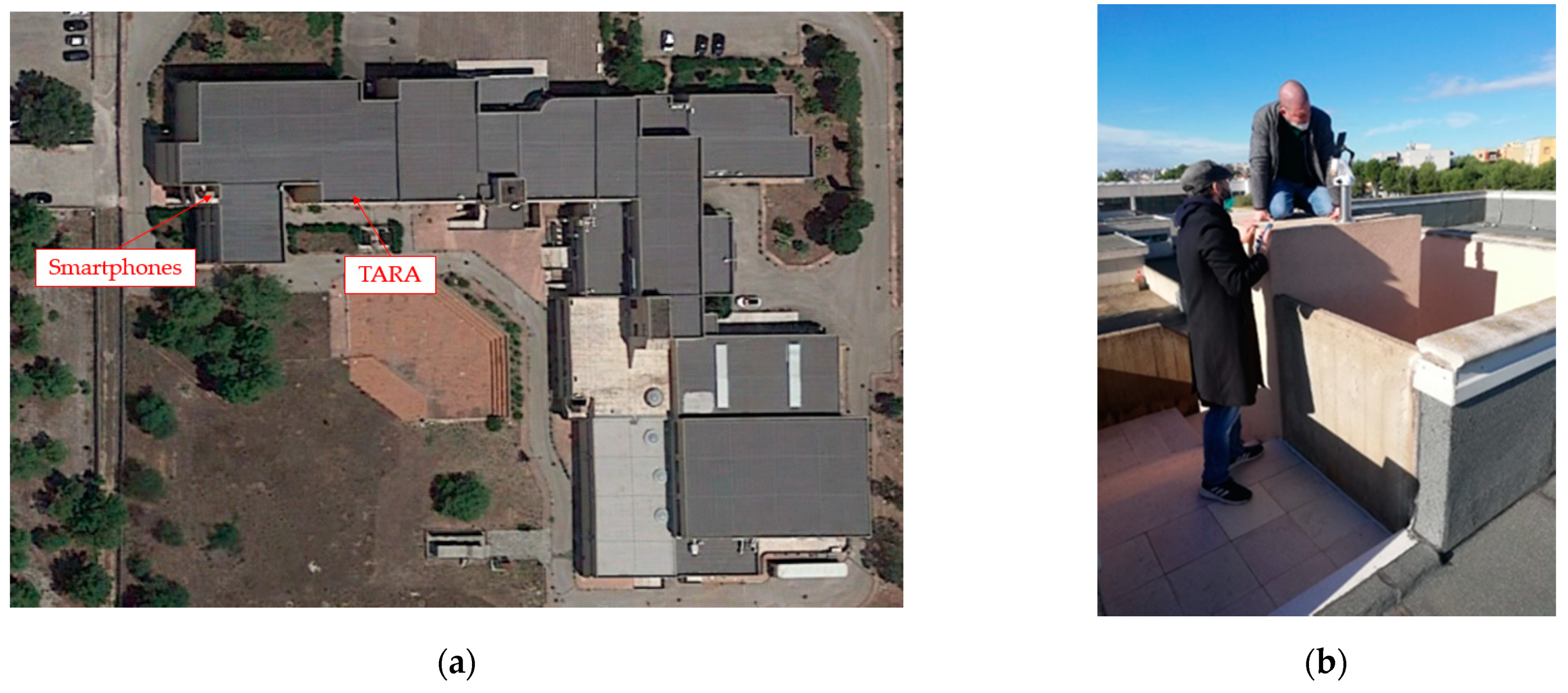
Data were collected in the static way over several days on the roof of the Polytechnic of Bari in the headquarters of Taranto, in South Italy (Figure 1a). The location on the roof of the building allowed observations to be made in open sky conditions. For data collection, the smartphones were positioned in the old vertex of a permanent GNSS network called FATA [23] (Figure 1b). Therefore, the FATA point is a place of known coordinates, stable and free of any external electromagnetic disturbances, as it has been monitored for several years.
The GNSS antenna of the smartphone is located in its upper left corner, as can be deduced from the manufacturer’s data sheet. For this reason, it was decided to position the smartphone in such a way as to obtain better acquisition of satellite data. The antenna of the permanent TARA GNSS station (described in Section 3.1) is located about 22 m (baseline) from the FATA station where the smartphone is positioned. The coordinates of the TARA and FATA stations are reported in Table 2.
3.3. Data Processing
The data were acquired on different days in order to obtain more datasets in different satellite configurations. The first dataset consists of the observations obtained in the first 5 min of each hour of observation; the second dataset consists of the first 10 min of each hour; the third dataset consists of the first 15 min of each hour; the fourth dataset consists of the first 30 min,; and the fifth dataset consists of 60 min of complete observation.
Each observation was processed with RTKPOST and CSRS-PPP. Static differential positioning with pseudorange measurements was performed by RTKPOST, using the permanent TARA GNSS station as a reference (base). CSRS-PPP was used to perform Single Point Positioning. The SPP was performed on single-frequency code observations and the data were mainly processed with a rapid ephemeris; the final ephemeris was used, if available. At the end of all processing, for each observation, the coordinates were obtained of the positioning of Xiaomi Mi 10 in Eastings () and Northing () in the WGS84-UTM system, and the ellipsoidal height Up () with their respective standard deviations (, and ). Following, the sub-datasets are shown for 5, 10, 15, 30 and 60 min:
Considering, as reference, the coordinates of the FATA (EFATA, NFATA, and UFATA), the positioning errors ΔEi, ΔNi, ΔUi of the Xiaomi Mi 10 were calculated with the following formulas:
The sub-datasets created, ΔE, ΔN, ΔU, take the following form:
where:
- i = 1, …, n;
- n is equal to the number of observations for 5, 10, 15, 30 and 60 min: n = 9 for the 5, 10 and 15 min datasets; n = 7 for the 30 and 60 min datasets.
Considering the positioning in DGNSS and SPP for each observation time, it is possible to create ten databases consisting of the sub-datasets: E, N, U, SDE, SDN, SDU, ΔE, ΔN, ΔU, as follows:
For each sub-dataset ΔE, ΔN, ΔU, a normality test of Shapiro–Wilk can be conducted, using the following formula [24]:
where:
- x(i) i-th is the smallest value (ΔE(i), ΔN(i), ΔU(i)) of the sub-dataset (ΔE, ΔN, ΔU);
- is the arithmetic mean of the values (ΔEi, ΔNi, ΔUi) of the sub-dataset (ΔE, ΔN, ΔU);
- ai is equal to
- m’ = m1, …, mn
- m1, …, mn are expected values of the ranks of a standardised random number;
- V is the matrix of the covariance of ranks.
Through RStudio software, the Shapiro–Wilk test can be easily performed, analysing the returns of the W and p values. The test aims to verify the following hypotheses:
- H0: Distribution of the dataset normal;
- H1: Distribution of the dataset not normal.
In establishing a threshold value equal to 0.05, the following occur:
- If the p-value > 0.05, the null hypothesis H0 is accepted;
- If the p-value < 0.05, the null hypothesis H0 is rejected.
According to the Shapiro–Wilks tests, the sub-datasets of ΔE, ΔN, ΔU for which normality is verified are represented by the normal distribution of Gauss:
Then, the arithmetic means for the sub-datasets ΔE, ΔN, ΔU were calculated, taking into account all the xi values (ΔEi, ΔNi, ΔUi) included in them, using the following formula:
To identify possible outliers in the sub-datasets, two methods were chosen. In the first method, the xi outliers of the sub-datasets ΔE, ΔN, ΔU were found and eliminated by applying the Tukey method [25,26,27].
Following the method, two fences, one lower and one upper, were identified:
where:
- Q1 is the first quartile;
- Q3 is the third quartile;
- IQR is the interquartile range equal to Q3 – Q1
In this way, it is possible to eliminate the xi values lower and higher than the two fences and, consequently, three new sub-datasets ΔEMm, ΔNMm, ΔUMm are generated. Normality tests were performed using Equations (14) and (17).
In the second method, the possible outliers xi are identified by applying an unsupervised classification algorithm called K-means, imposing some exclusion conditions based on distance [28]. The concept is to consider as outliers the values farthest from the cluster centres.
- Choice of the number of classes K (K = 2);
- Setting of a mean cluster centre Ci (i = 1, 2) for elements xi of classes K;
- Assignment of the elements xi to one of the two classes Ci respecting the following condition:
- 4.
- Calculation of the new cluster centres:
- 5.
- If the clustering remains unchanged for two successive steps, it ends. Otherwise, it restarts from step 2.
After clustering, three exclusion conditions are imposed on the elements xi of the sub-datasets ΔE, ΔN, ΔU:
- If a cluster has a number of elements greater than 2, xi > 2, the element farthest from the cluster centre is deleted respecting the following condition:
- 2.
- If a cluster has a number of elements equal to 2, no element is eliminated since both are equidistant from Ci;
- 3.
- If a cluster consists of only one element, only that element is deleted from the sub-dataset.
If the sub-datasets consist of few values, it is possible to establish simple exclusion rules, while in the case of larger datasets, more elaborate exclusion rules can be imposed [28]. Using the method above, the elements xi, considered outliers, are eliminated, and three new sub-datasets ΔEKm, ΔNKm, ΔUKm can be created. Then, for each new sub-dataset we performed the normality test, using Equations (14) and (17).
The mean values for all data subsets (ΔE, ΔN, ΔU, ΔEMm, ΔNMm, ΔUMm and ΔEKm, ΔNKm, ΔUKm) were tabulated, analysed and compared to each other to determine normal distributions, standard deviations and positioning errors.
Linear regressions were implemented to identify possible correlations between mean values and observation times.
Once the level of accuracy achieved by the smartphones is identified, it can be evaluated and tested by means of an application in the field of surveying.
4. Results
4.1. Normality Test
This section is dedicated to evaluating the p-values and collecting in tables the sub-datasets that have passed the normality test.
Table 3 reports verification, by normality test, for the sub-datasets ΔE, ΔN, ΔU, ΔEMm, ΔNMm, ΔUMm and ΔEKm, ΔNKm, ΔUKm for positioning in DGNSS and for the five observation times. With a threshold value of 0.05, the sub-datasets not verified are ΔE for 5 and 15 min, ΔU for 15 min, ΔEMm for 5 min, and ΔEKm for 5 and 15 min.
From the observation of Table 3, it is possible to notice that there is no relationship between the length of the observation time and the verification by the normality test for DGNSS positioning.
Table 4 reports the verification of the normality test for the sub-datasets for Single Point Positioning (SPP) and for the five observation times. With a threshold value of 0.05, the sub-datasets not verified are ΔE for 30 min, ΔN for 15 min, ΔEKm for 5 min, ΔNKm and ΔUKm for 10 and 15 min.
Furthermore, for Single Point Positioning, a relationship between the duration of the observation time and the verification of the normality test is not evident.
4.2. Evaluation of DGNSS and SPP Standard Deviation
In this section, the standard deviations of the sub-dataset ΔE, ΔN, ΔU are collected for the various observation times and evaluated through tables and, subsequently, by the application of the linear regression. In this way, it is possible to evaluate functional relationships between standard deviations and length of observation sessions.
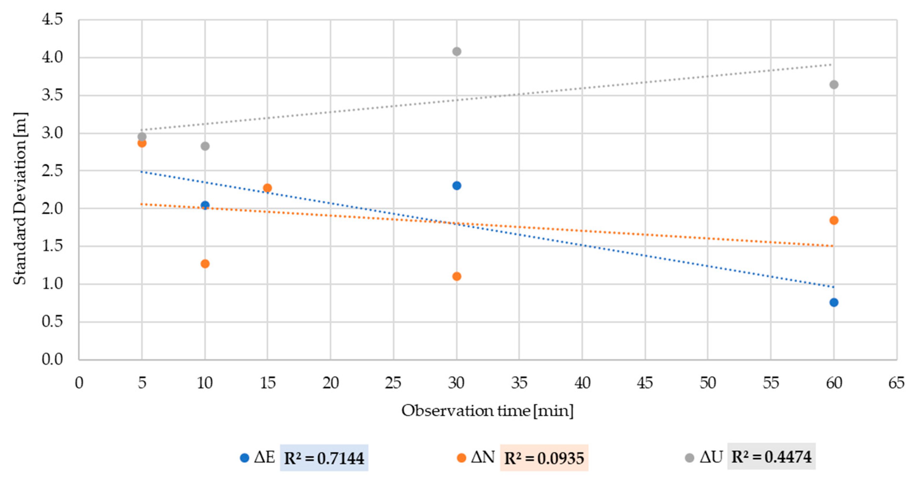
Table 5 summarises the standard deviations in relation to DGNSS session length positioning of the several sub-datasets. Figure 2 shows the behaviour of the standard deviation for ΔE, ΔN and ΔU sub-dataset of DGNSS positioning over time and the R2 values for the related sub-datasets.
Observing Table 5 and Figure 2, it can be seen that there is a strong linear relationship between standard deviation DGNSS and observation time only for ΔE (R2 = 0.71) [30].
In Appendix A (Figure A1, Figure A2 and Figure A3), through the normal distributions, it is possible to evaluate the relationships between standard deviation and observation times.
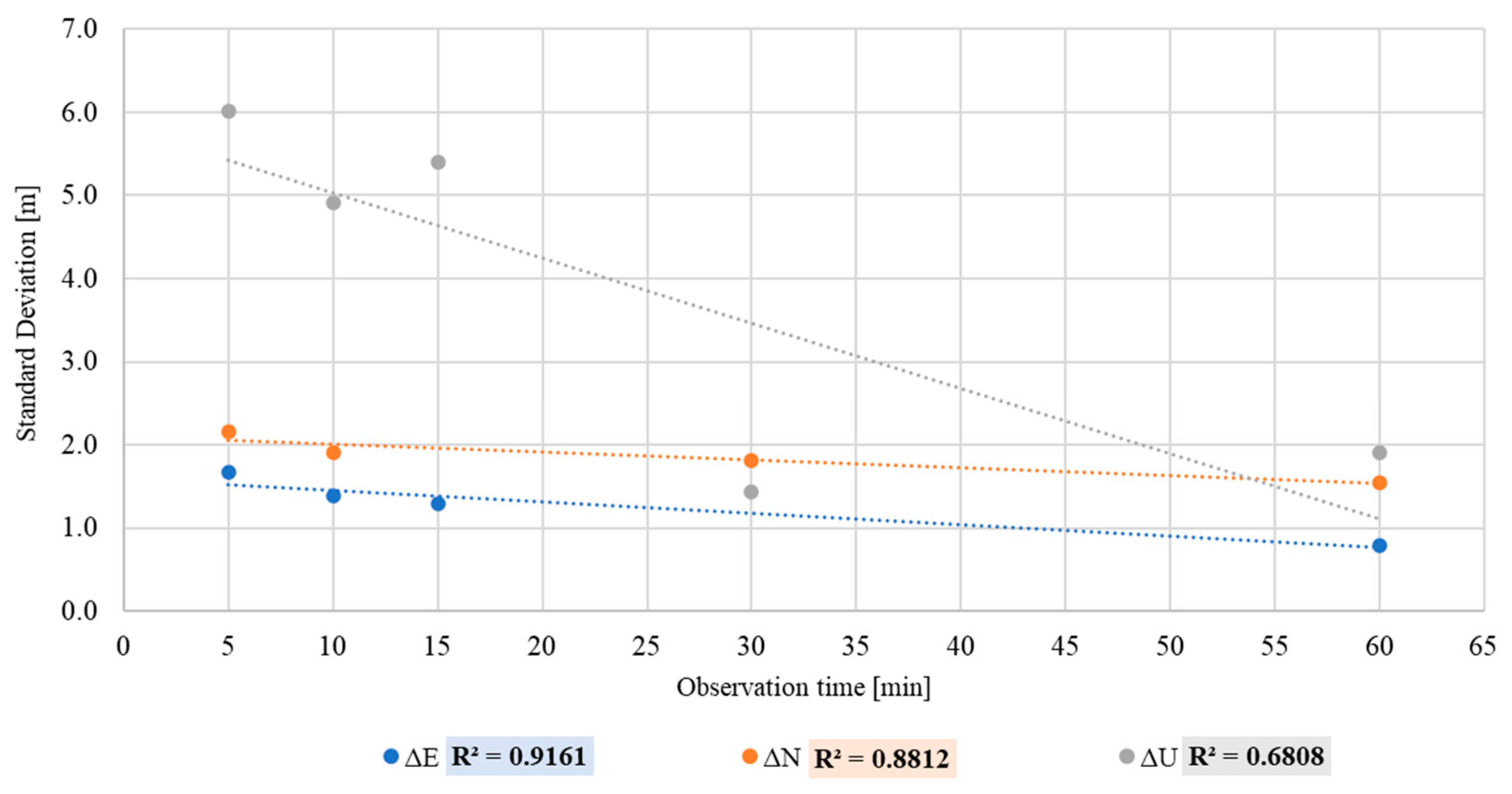
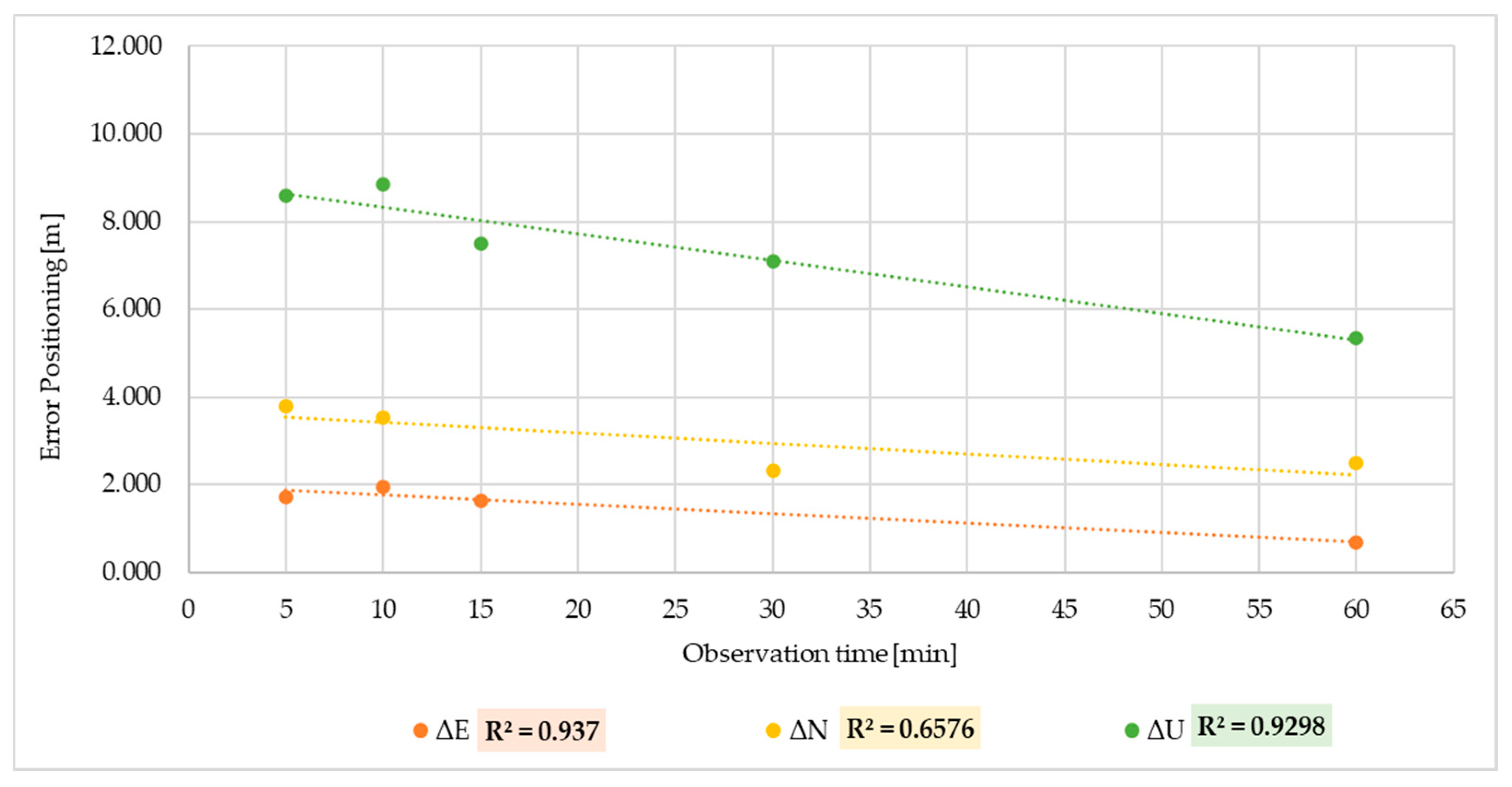
Table 6 summarises the standard deviations for all observations in SPP. Figure 3 shows the behaviour of the standard deviation for ΔE, ΔN and ΔU sub-dataset of Single Point Positioning over the time and reports the R2 values for the sub-datasets ΔE, ΔN and ΔU.
Regarding the SPP, unlike the DGNSS, it is possible to note a linear relationship between the standard deviations and observation times for all three sub-datasets. ΔE and ΔN have a strong relationship, with R2 values equal to 0.92, 0.88, and ΔU demonstrates a moderate relationship, with an R2 = 0.68 [30].
The relationships between standard deviations and observation times are shown in Appendix B (Figure A4, Figure A5 and Figure A6).
4.3. Evaluation of DGNSS Positioning Error
In this section, the possible functional relationships between positioning errors and observations session are evaluated through the verification of fitting of linear regressions.
Table 7, Table 8 and Table 9 report the means of DGNSS positioning errors in Easting, Northing, and Up, respectively. The means refer to the sub-datasets ΔE, ΔN, ΔU: the means obtained from the sub-datasets ΔEMm, ΔNMm, ΔUMm and the means of the sub-datasets ΔEKm, ΔNKm, ΔUKm. Again, the values of the means were not reported where the normality test was not verified.
From Table 7, Table 8 and Table 9, we can evaluate the DGNSS mean positioning error. In particular, the minor Easting error (ΔEMm = 1.471 m) was obtained at 15 min for the sub-dataset ΔEMm. This result suggests for ΔEMm non-dependency on the duration of observation times with the achievable error; in fact, it is possible to observe an error value of 1.875 m for an acquisition of 60 min.. This result is not consistent with what is expected in the GNSS measurements with topographic receivers. For the Easting coordinate, at 60 min, the greatest error was detected for ΔE and ΔEMm and the lowest error was equal to 1.698 m for ΔEKm.
For the North position, the lowest error was reached at 10 min for the subsets ΔN and ΔNMm and was equal to 2.016, but also, in this case, for the 60-min acquisition, the error did not decrease (ΔN and ΔNMm = 2.489 m).
The lowest positioning error in the Up coordinate was obtained for 15 min for ΔUMm and ΔUKm and was equal to 3.087 m, while at 60 min, the error was equal to 3.572 m for ΔUKm. This was also the minor Up error at 60 min between the three sub-datasets, while the greatest error at 60 min in Up was equal to 3.579 m for ΔUMm and ΔU.
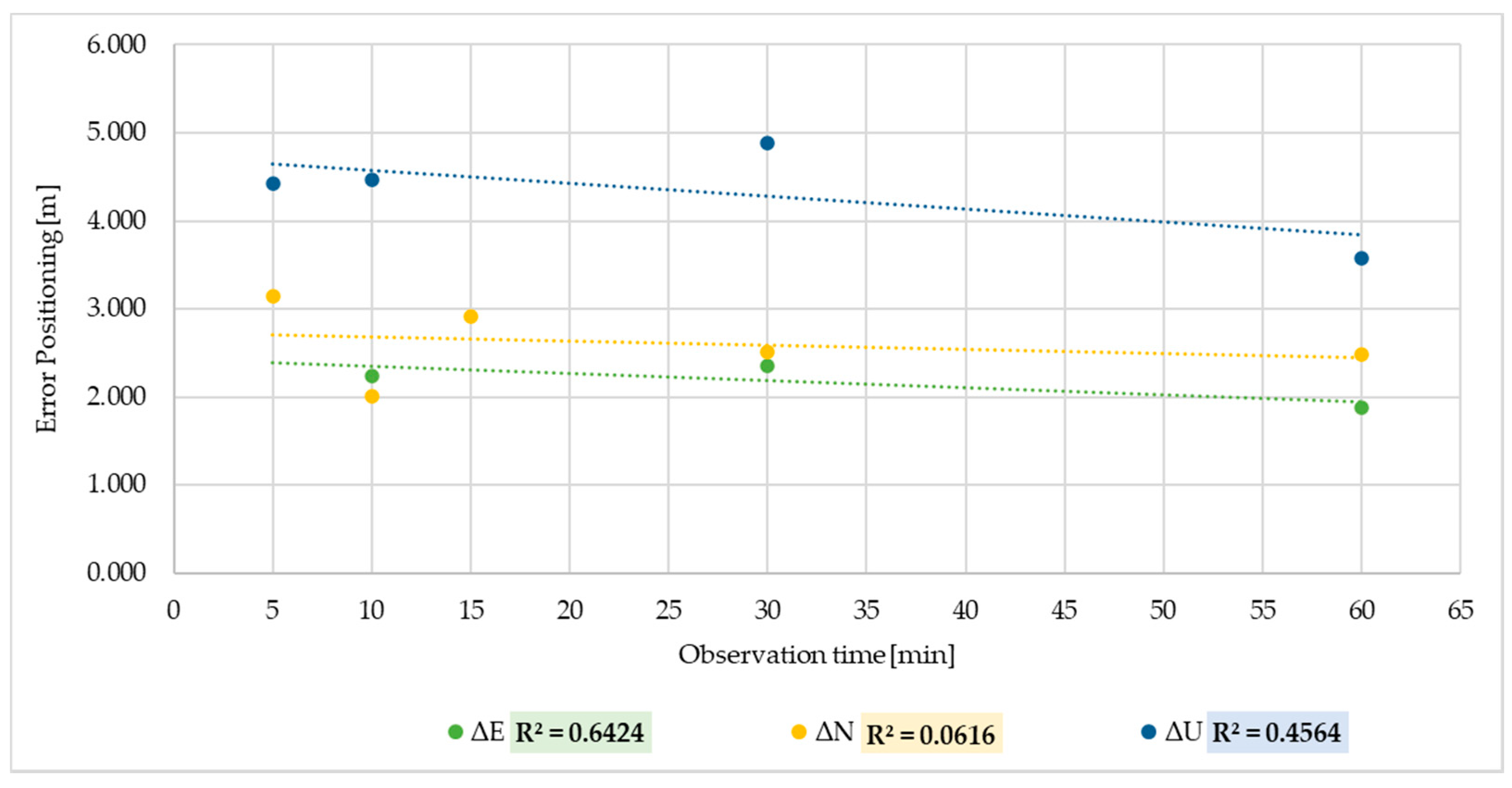
Through the study of linear regressions between the means of all sub-datasets of the DGNSS positioning errors and the observation times, it is possible to note a general weak relationship with values of R2 < 0.5, for the most part, of the sub-datasets. Only the sub-datasets ΔE and ΔEKm show a linear relationship between variables, with R2 values equal to 0.64 (moderate relationship) and 0.85 (strong relationship), respectively (Figure 4).
4.4. Evaluation of Single Point Positioning Error
The analysis of SPP in Easting, Northing and Up are summarised in the Table 10, Table 11 and Table 12. In particular, the tables show the means referring to sub-datasets ΔE, ΔN, and ΔU: ΔEMm, ΔNMm, ΔUMm and ΔEKm, ΔNKm, ΔUKm. In accordance with Table 4, the values of the means were not reported where the normality test was not verified.
From Table 10, Table 11 and Table 12, it is possible to obtain information about the mean error for Single Point Positioning. For the Easting coordinate, at 60 min, the major error is equal to 0.706 m for the ΔEKm sub-dataset, while the minor one is equal to 0.439 m for ΔEMm. For the Northing positioning at 60 min, the major error is committed for the ΔN sub-dataset and is equal to 2.509 m, while the minor Northing error is, instead, equal to 1.984 m for ΔNMm and ΔNKm. At 60 min, the major positioning error Up is recorded for sub-databases, ΔUMm and ΔUKm, and is equal to 5.916 m; the minor one is equal to 5.346 m for the sub-database ΔU.
By observing the R2 values, it is possible to assess the functional relationships between the averages of the SPP errors (for each sub-dataset) and the acquisition time; in particular, linear regression was used for all sub-datasets.
Unlike DGNSS positioning, by observing the coefficient of determination R2, it is possible to note that for the SPP, there is generally a linear relationship between the observation times and positioning errors that is between moderate and strong.
For a more cautious assessment of the degree of relationship between variables, it is advisable to analyse the R2 values for the sub-datasets according to the positionings of Easting, Northing and Up.
The sub-datasets for Easting, ΔE, ΔEMn and ΔEKm, show the strongest and most consistent linear functional relationship between variables, with R2 values equal to 0.94, 0.88 and 0.92. For Northing positioning, the sub-dataset ΔNKm demonstrates a strong relationship between variables with a value of R2 = 0.94; however, ΔN and ΔNMn, with values equal to 0.66 and 0.58, instead demonstrate a moderate relationship between variables. As a precaution, a moderate relationship between the variables can be assumed, but of course, it is not as strong as that for the Easting positioning. The absolute highest R2 value is expressed by the Up sub-dataset ΔUKm (R2 = 0.98), and not to be underestimated is the ΔU with an R2 = 0.93 but it is equally true that the Up positioning also expresses the lowest value with ΔUMm (R2 = 0.49). Even for the UP positioning, it can be conservatively assumed that there is no more than a moderate linear relationship between the variables [30].
Figure 5 shows an example of the linear regression performed for the sub-datasets ΔE, ΔN and ΔU in Single Point Positioning.
5. Discussion
Smartphone positioning has shown limitations in the accuracy of its results compared to those obtained with traditional geodetic instruments. However, the aim of this work was not to compare smartphones with high-performance GNSS geodetic instruments, but rather to define possible smartphone applications. It should be pointed out that although the smartphone is equipped with hardware for dual frequency carrier phase acquisition, this is not stored in the app used in the experimentation. Consequently, the measurements were carried out with only the information of the codes present in the various constellations. The lack of information of the phase measurement could be due to limitations imposed by the Android operating system.
Tests with the three smartphones showed no substantial differences in accuracy and precision. The positioning errors of the three devices were processed for observation times of one, five and ten minutes, and the SPP and DGNSS solutions were fully compared. In particular, for the Huawei and OPPO smartphones, at one minute, there were errors in the order of meters and the positioning error decreased when the observation increased to five and to thirty minutes. Comparing the positioning errors at 60 min, it was observed that SPP is more advantageous than DGNSS in determining the Easting coordinate, unlike DGNSS, which is preferable to SPP for Up positioning. In Appendix C (Figure A7), it is possible to see a spatial distribution of the error obtained for SPP and DGNSS.
In particular, the best planimetric positioning was obtained for the SPP sub-datasets whose outliers were eliminated with the Tukey method; the mean of Easting and Northing positioning errors were equal to ΔEMn = 0.439 m and ΔNMn = 1.984. Good results were also obtained with the sub-datasets whose outliers were eliminated by clustering: in this case, the mean of Easting and Northing positioning errors were equal to ΔEKn = 0.706 m and ΔNKn = 1.984 m. The sub-datasets not treated with the elimination of the outliers instead showed mean positioning errors equal to ΔE = 0.700 m and ΔNMn = 2.509 m. The best Up positioning was obtained with the DGNSS method, with a position error ΔUKn = 3.57 m; the other two sub-datasets ΔU and ΔUMn instead obtained a mean positioning error equal to 3.58 m.
The study of linear regressions shows that the accuracy and precision of SPP improves as the observation time increases, which leads the user to choose this mode if the observation can take place over a long period of time. In the DGNSS, no direct correlation between observation time and accuracy was found.
The choice in location of the smartphones was made to use very short baselines (less than 1 km) in order to assess only the fixed amount of error without considering the variation due to the distribution of error as a function of distance. It was verified, considering another permanent GNSS station with baselines of about 50 km (Avetrana site), that DGNSS positioning errors do not vary significantly for positioning with code pseudoranges.
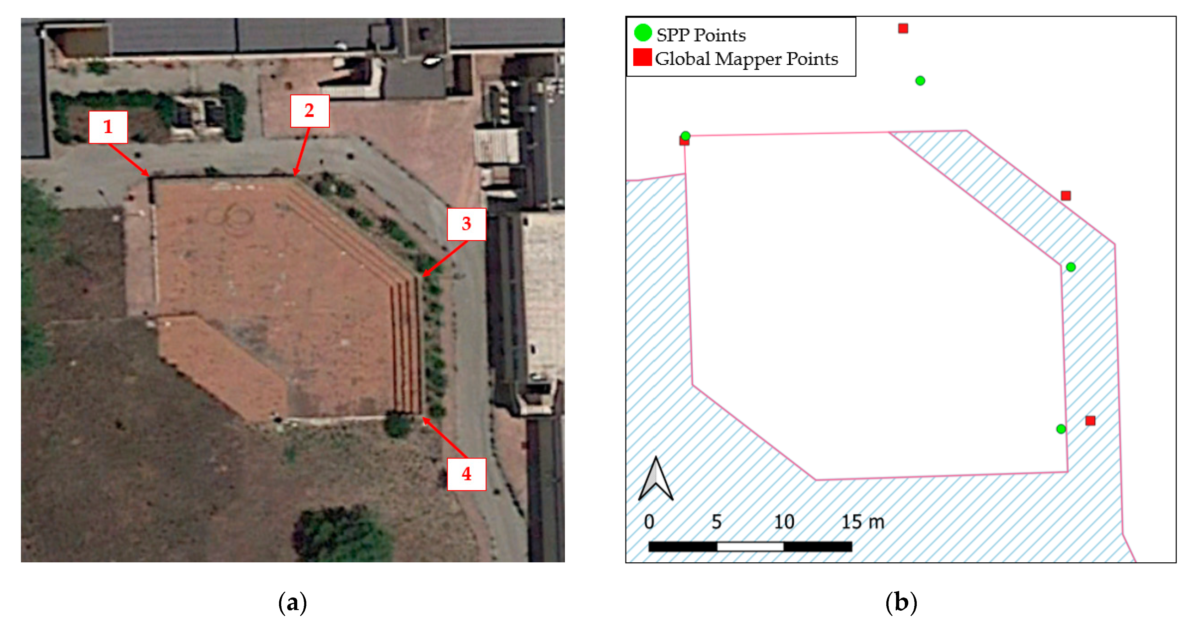
In order to test the applicability of the results obtained, a smartphone survey of the wall of a small amphitheatre was carried out. The survey consisted of the acquisition of four vertices of the amphitheatre with the Xiaomi Mi 10 (Figure 6) and observation times of 1 min with the Geo++ Rinex Logger for subsequent post processing in SPP. At the same time, the same vertices were acquired in real time with the Global Mapper Mobile app and with the same acquisition times. In Table 13 and Figure 6, it can be observed that SPP obtained better positioning results in 100% of the cases, proving to be better than Global Mapper Mobile positioning in real time.
6. Conclusions
In this paper, we present a statistical analysis method to evaluate the accuracy and precision of GNSS positioning of smartphones, using only pseudorange measurements. The choice was made to extend such methods to any device using pseudorange only since carrier phase measurements are not always available on all devices.
Two methods were described for the detection and elimination of outliers in the positioning data, namely, the Tukey and the K-means methods, which can improve the positioning accuracy of mobile devices.
The K-means method can be further investigated in order to improve the positioning performance of smartphones through artificial intelligence; therefore, the authors propose further studies in this research direction.
The comparative study of DGNSS and SPP methods showed that SPP is more accurate for medium to long observation times, while DGNSS is more efficient in the short term.
The results obtained could be aimed at applications in GIS for smartphones, allowing, for example, the creation of citizen science experiments (environmental, extended heritage monitoring, etc.), quickly and relatively accurately.
The application conducted using a smartphone app showed that it is possible to improve accuracy if a tool is implemented to analyse and process corrections in real time, such as a CSRS-PPP service. This implementation could significantly improve GNSS positioning in smartphone GIS and identify developments for further applications.
Author Contributions
Conceptualisation, M.P., D.C., G.V. and V.S.A.; methodology, M.P., D.C., G.V. and V.S.A.; software, M.P., D.C., G.V. and V.S.A.; validation, M.P., D.C., G.V. and V.S.A.; formal analysis, M.P., D.C., G.V. and V.S.A.; investigation, M.P., D.C., G.V. and V.S.A.; data curation, M.P., D.C., G.V. and V.S.A.; writing—original draft preparation, M.P., D.C., G.V. and V.S.A.; writing—review and editing, M.P., D.C., G.V. and V.S.A.; visualisation, M.P., D.C., G.V. and V.S.A. All authors contributed equally to the research and writing of the manuscript. All authors have read and agreed to the published version of the manuscript.
Funding
This research received no external funding.
Institutional Review Board Statement
Not applicable.
Informed Consent Statement
Not applicable.
Data Availability Statement
Not applicable.
Acknowledgments
This research was carried out in the project: PON “Ricerca e Innovazione” 2014–2020 A. I.2 “Mobilità dei Ricercatori” D.M. n. 407-27/02/2018 AIM “Attraction and International Mobility” (AIM1895471–Line 1).
Conflicts of Interest
The authors declare no conflict of interest.
Abbreviations
| E | sub-dataset of smartphone Easting positioning coordinates. |
| N | sub-dataset of smartphone Northing positioning coordinates. |
| U | sub-dataset of smartphone Up positioning. |
| SDE | sub-dataset of the standard deviation of smartphone Easting positioning. |
| SDN | sub-dataset of the standard deviation of smartphone Northing positioning. |
| SDU | sub-dataset of the standard deviation of smartphone Up positioning. |
| RMS | Root Mean Square. |
| NTNV | Normality Test Not Verified. |
| ΔE | sub-dataset of Easting positioning errors between smartphone and FATA. |
| ΔN | sub-dataset of Northing positioning errors between smartphone and FATA. |
| ΔU | sub-dataset of Up positioning errors between smartphone and FATA. |
| ΔEMm | sub-dataset of Easting positioning errors between smartphone and FATA, the outliers were eliminated by Tukey’s method. |
| ΔNMm | sub-dataset of Northing positioning errors between smartphone and FATA, the outliers were eliminated by Tukey’s method. |
| ΔUMm | sub-dataset of Up positioning errors between smartphone and FATA, the outliers were eliminated by Tukey’s method. |
| ΔEKm | sub-dataset of Easting positioning errors between smartphone and FATA, the outliers were eliminated by K-Means algorithm. |
| ΔNKm | sub-dataset of Northing positioning errors between smartphone and FATA, the outliers were eliminated by K-Means algorithm. |
| ΔUKm | sub-dataset of Up positioning errors between smartphone and FATA, the outliers were eliminated by K-Means algorithm. |
Appendix A
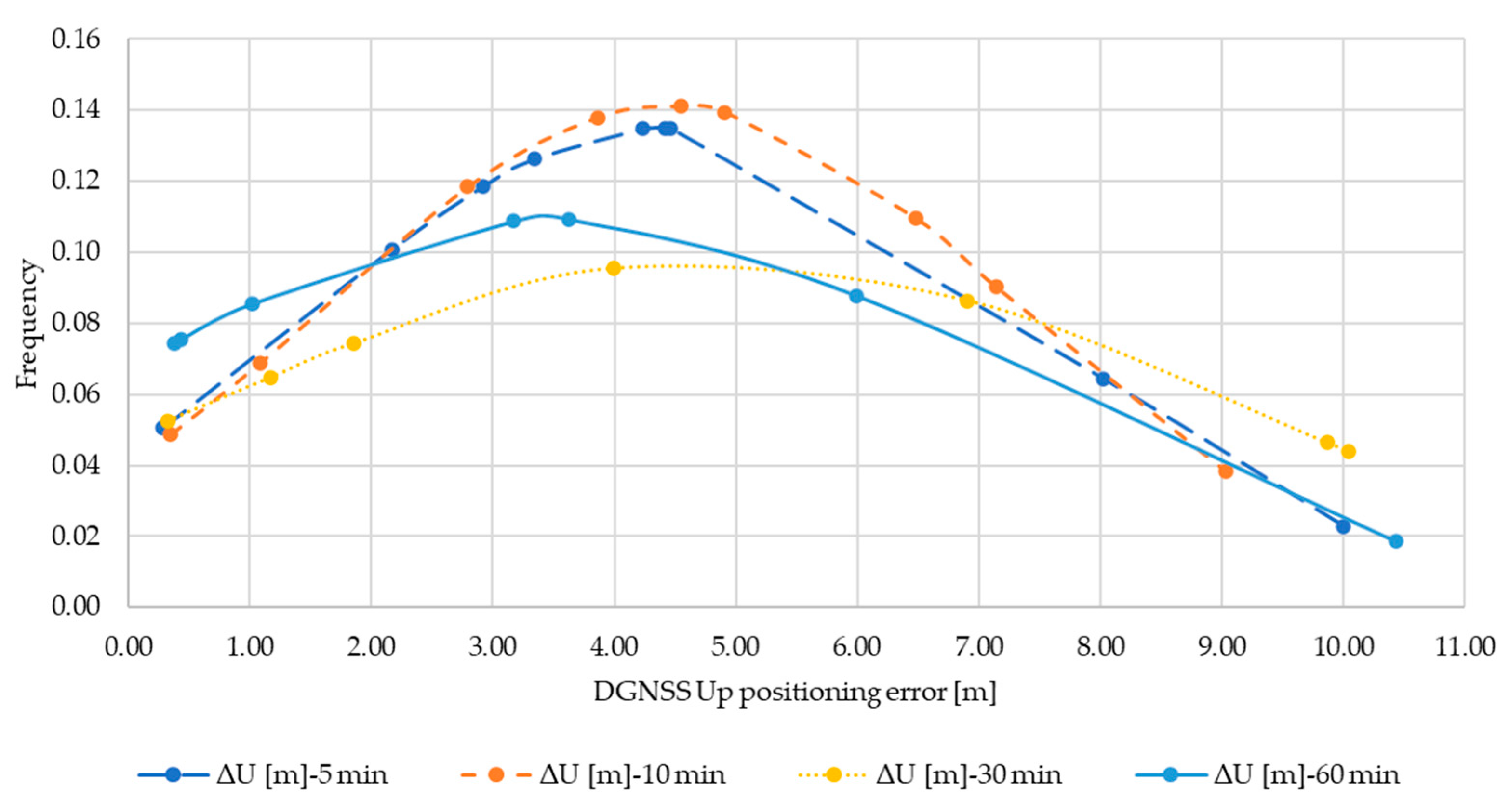
In the following figures are collected the normal distributions of the sub-datasets ΔE (Figure A1), ΔN (Figure A2) and ΔU (Figure A3), derived from DGNSS positioning for observations of 5, 10, 15, 30 and 60 min. It is possible to note the lack of normal distributions ΔE for 5 min and 15 min and ΔU for 15 min. These distributions were not reported, as the condition of normality of the distribution was not verified according to Table 3.
Figure A1.
Normal distribution ΔE for DGNSS.

Figure A2.
Normal distribution ΔN for DGNSS.

Figure A3.
Normal distribution ΔU for DGNSS.

Appendix B
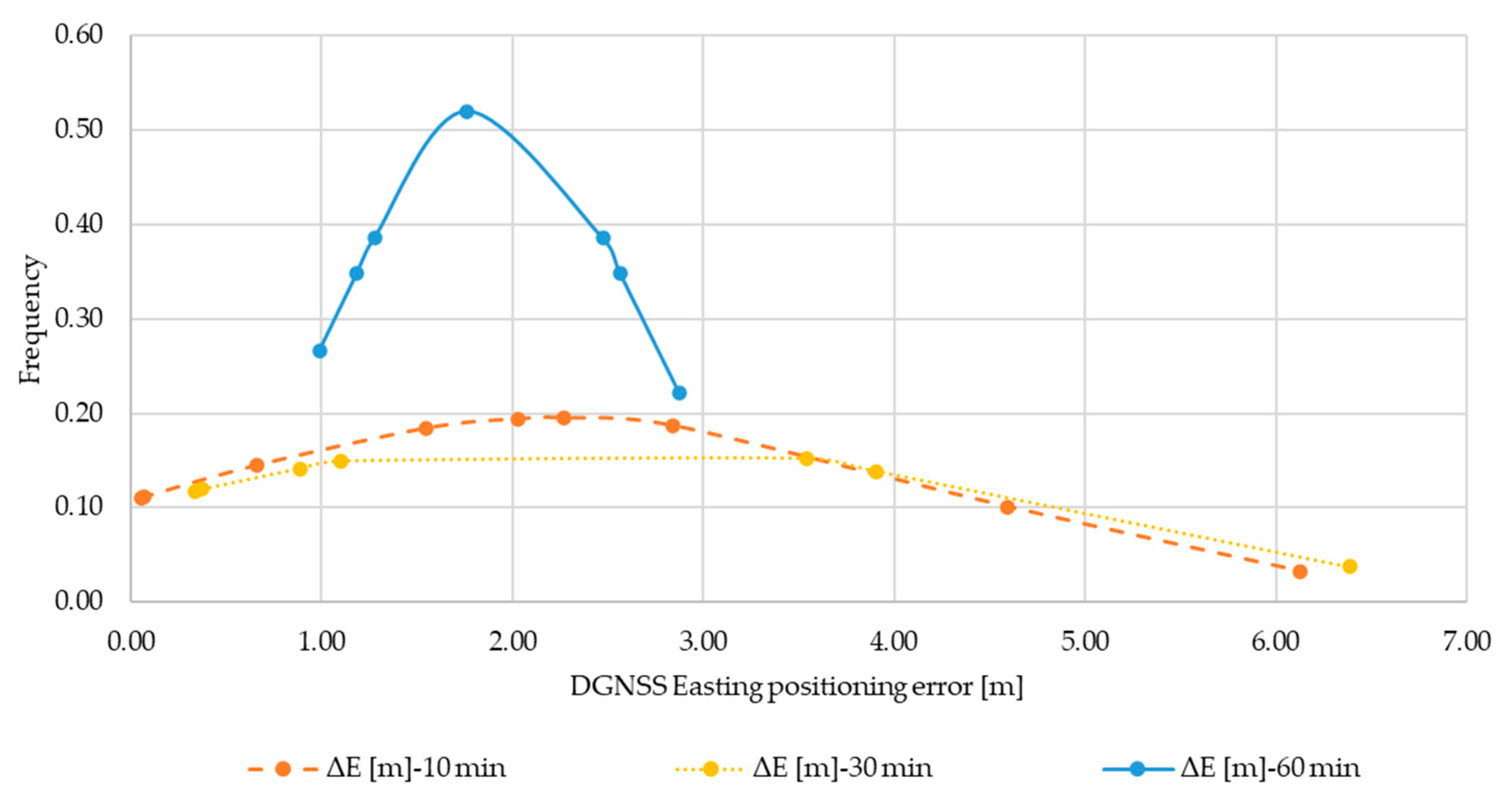
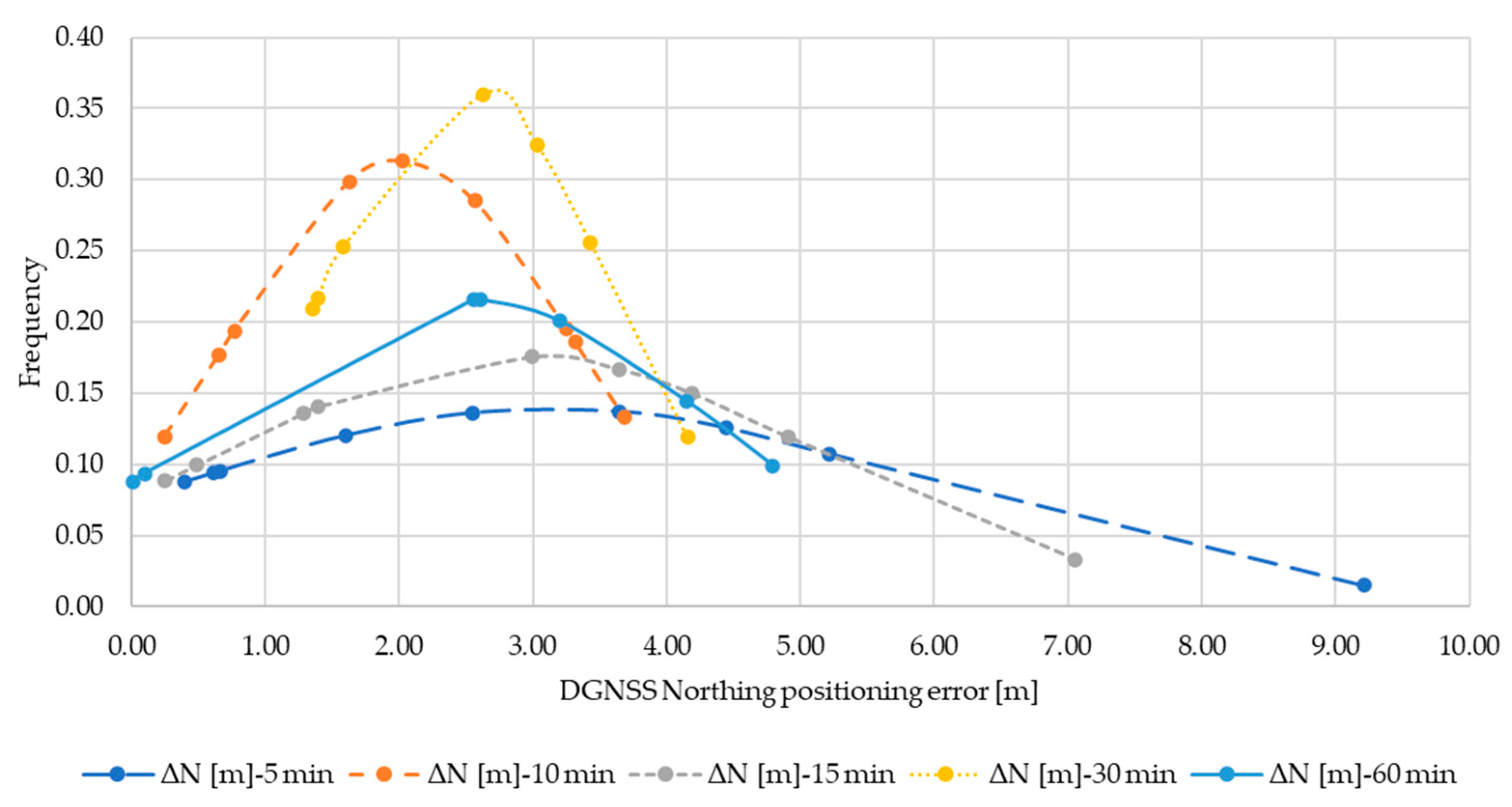
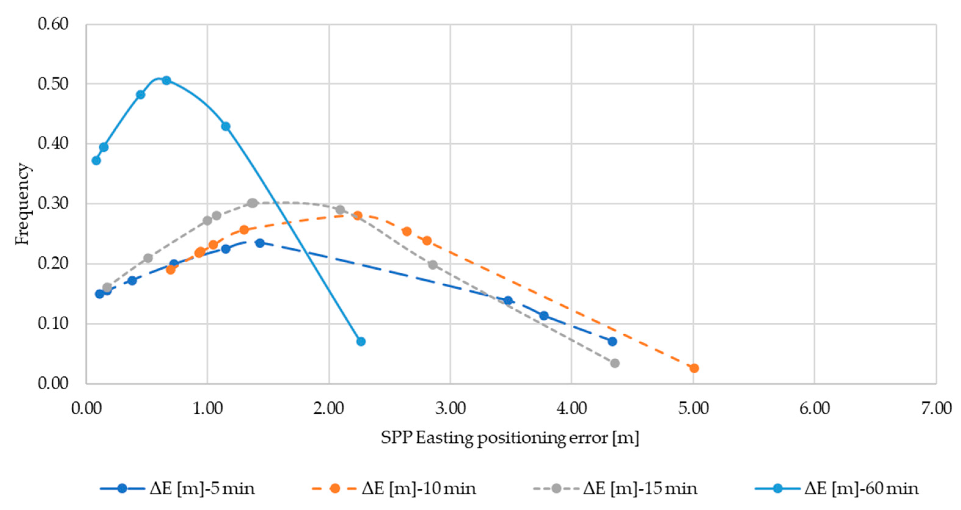
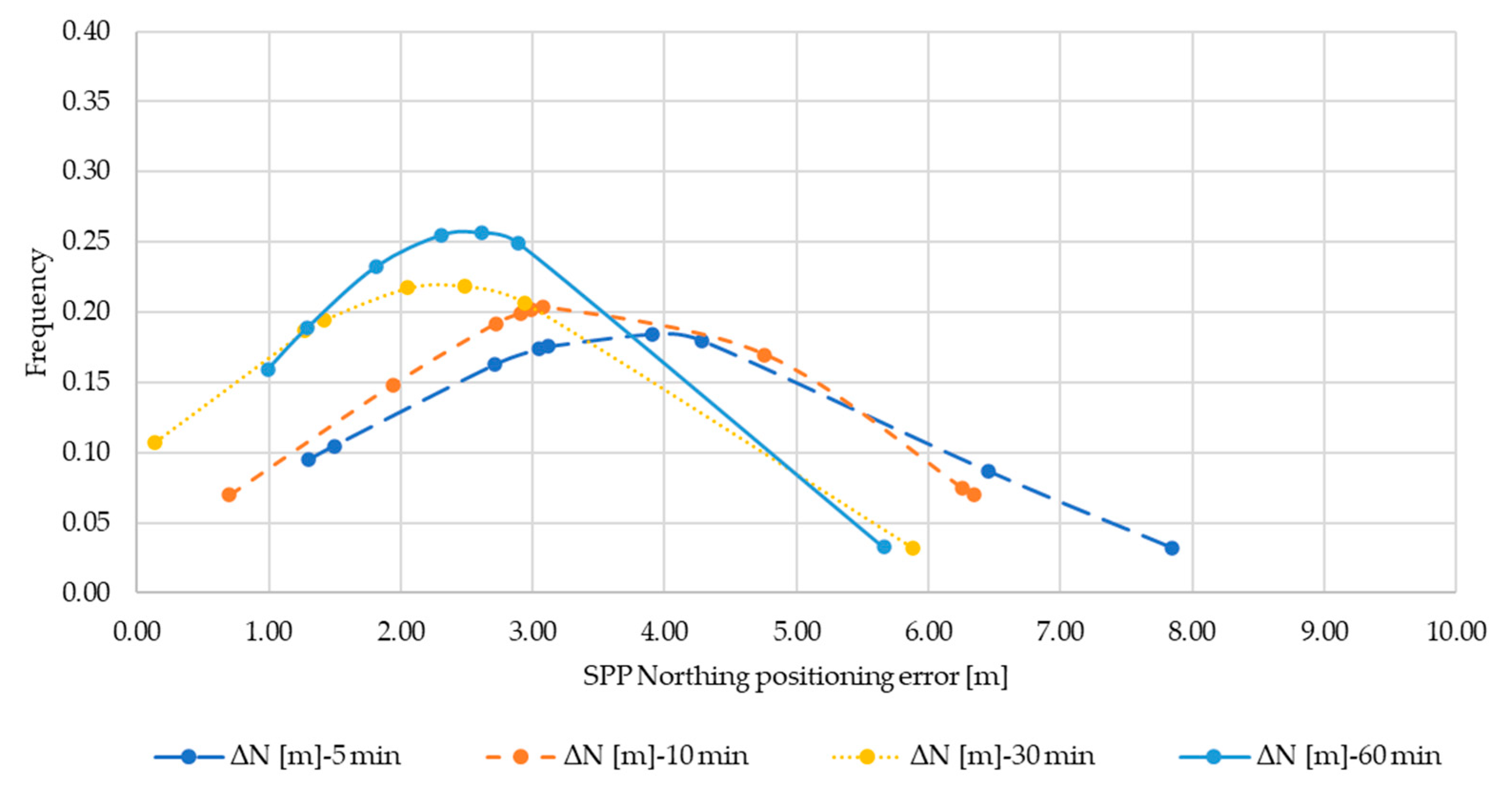
Below are shown the normal distributions of the ΔE (Figure A4), ΔN (Figure A5), ΔU (Figure A6) sub-datasets resulting from Single Point Positioning for 5, 10, 15, 30 and 60 min observations. The distributions of ΔE for 30 min, and ΔN for 15 min are omitted since the normal condition was not verified against the results of the test (see Table 4).
Figure A4.
Normal distribution ΔE for SPP.

Figure A5.
Normal distribution ΔN for SPP.

Figure A6.
Normal distribution ΔU for SPP.

Appendix C
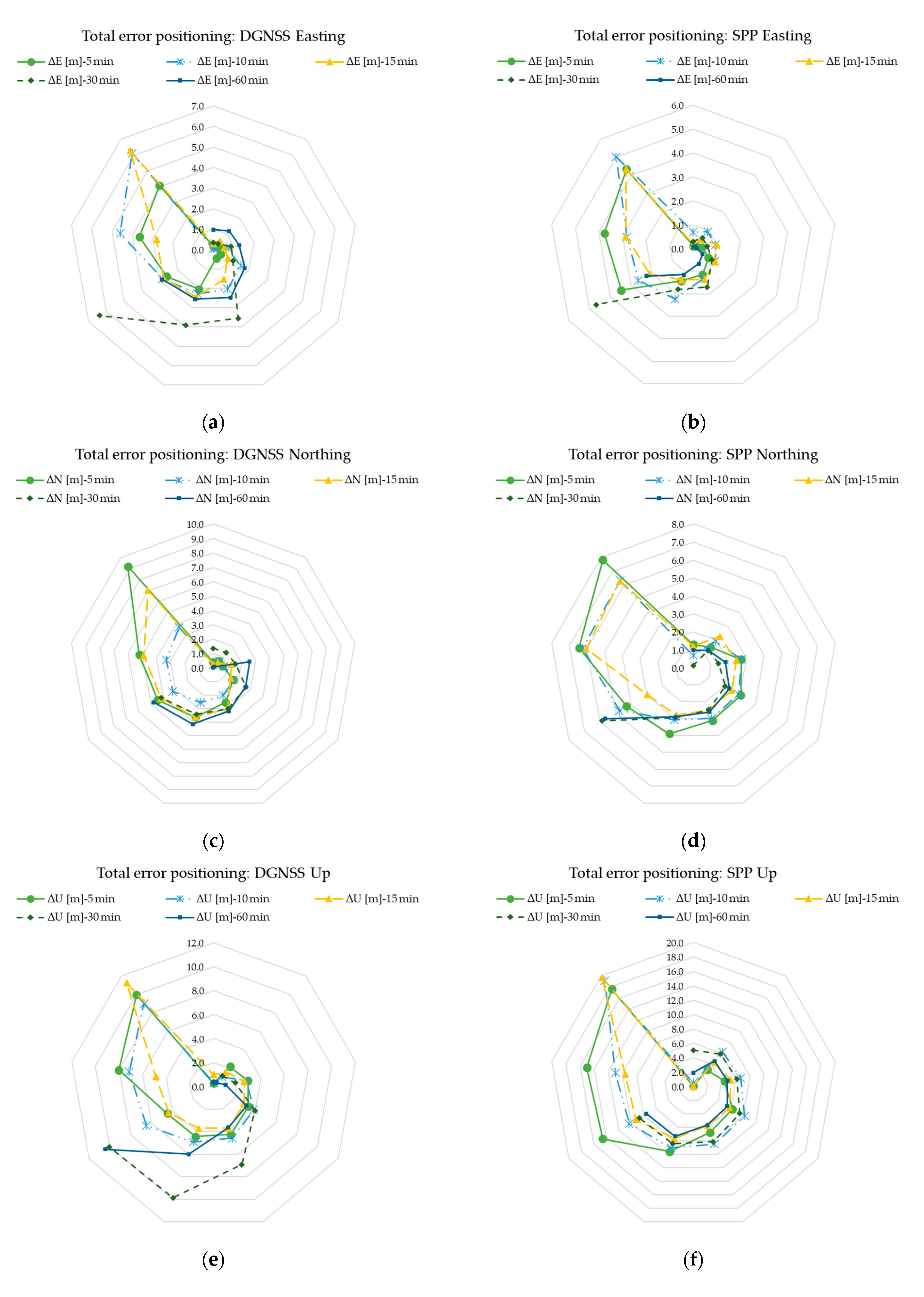
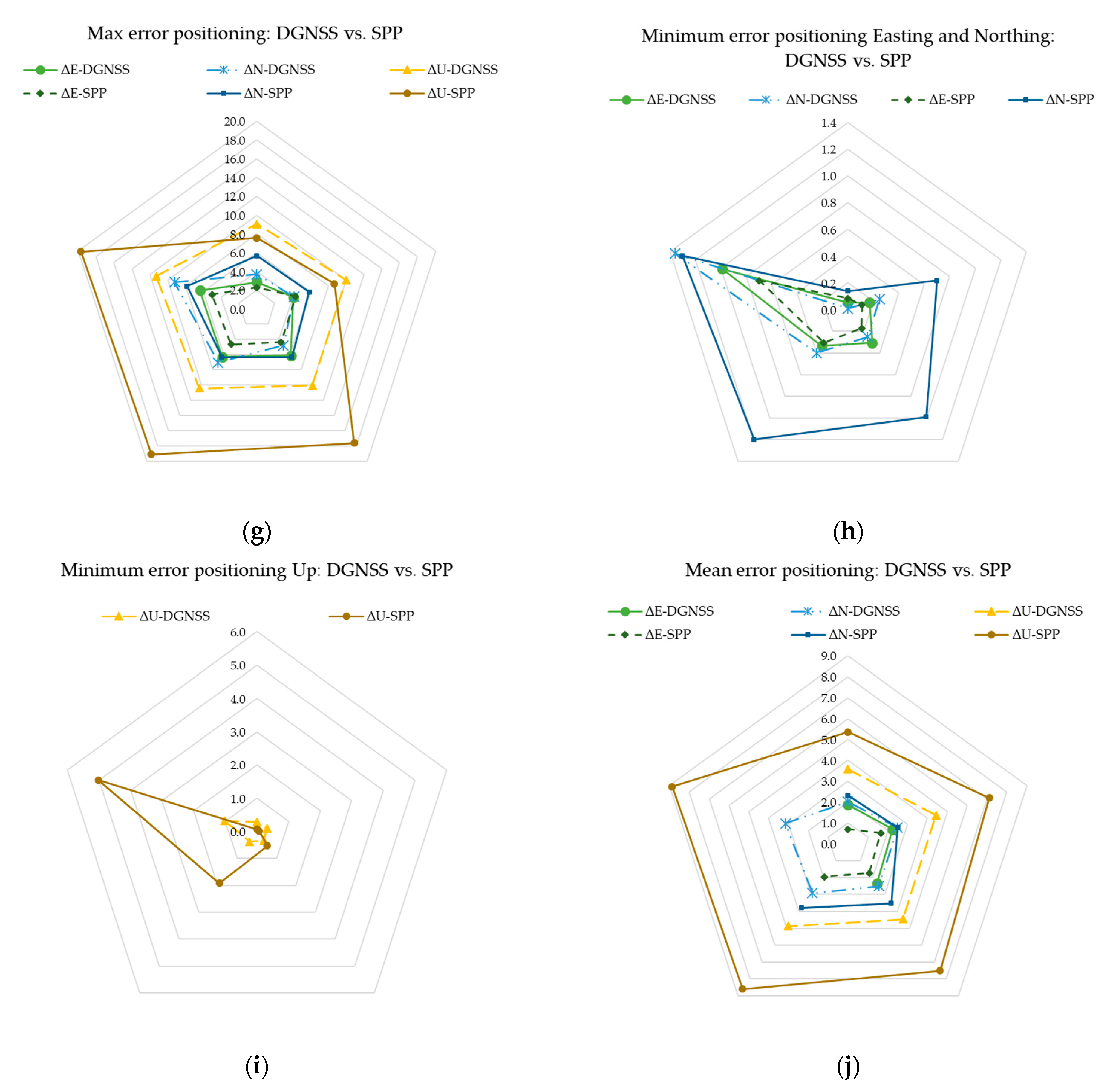
The DGNSS and SPP positioning strategies obtained by Xiaomi were compared (Figure A7). The radar graphics allow the comparison of the two methods through the visual exploration of data; the point of known coordinates (FATA) is positioned in the centre.
Figure A7.
Comparison of the positioning errors of the sub-datasets ΔE, ΔN, ΔU: (a) total DGNSS positioning error for the sub-dataset ΔE, (b) total SPP error for the sub-dataset ΔE, (c) total DGNSS positioning error for the sub-dataset ΔN, (d) total SPP error for the sub-dataset ΔN, (e) total DGNSS positioning error for the sub-dataset ΔU, (f) total SPP error for the sub-dataset ΔU, (g) comparison between the maximum positioning errors for all observation times, (h) comparison between the minimum planimetric positioning errors for all observation times, (i) comparison between the minimum up positioning errors for all observation times, (j) comparison between the mean positioning errors for all observation times.


References
- European GNSS Agency. White Paper on Using GNSS Raw Measurements on Android Devices. 2017. Available online: https://www.euspa.europa.eu/newsroom/news/available-now-white-paper-using-gnss-raw-measurements-android-devices (accessed on 3 May 2021).
- Dabove, P.; Di Pietra, V.; Piras, M. GNSS Positioning Using Mobile Devices with the Android Operating System. ISPRS Int. J. Geoinf. 2020, 9, 220. [Google Scholar] [CrossRef] [Green Version]
- Gioia, C.; Borio, D. Android Positioning: From Stand-Alone to Cooperative Approaches. Appl. Geomat. 2020, 1–22. [Google Scholar] [CrossRef]
- Zhang, X.; Tao, X.; Zhu, F.; Shi, X.; Wang, F. Quality Assessment of GNSS Observations from an Android N Smartphone and Positioning Performance Analysis Using Time-Differenced Filtering Approach. Gps Solut. 2018, 22, 1–11. [Google Scholar] [CrossRef]
- Zhang, K.; Jiao, W.; Wang, L.; Li, Z.; Li, J.; Zhou, K. Smart-RTK: Multi-GNSS Kinematic Positioning Approach on Android Smart Devices with Doppler-Smoothed-Code Filter and Constant Acceleration Model. Adv. Space Res. 2019, 64, 1662–1674. [Google Scholar] [CrossRef]
- Liu, W.; Shi, X.; Zhu, F.; Tao, X.; Wang, F. Quality Analysis of Multi-GNSS Raw Observations and a Velocity-Aided Positioning Approach Based on Smartphones. Adv. Space Res. 2019, 63, 2358–2377. [Google Scholar] [CrossRef]
- Guo, L.; Wang, F.; Sang, J.; Lin, X.; Gong, X.; Zhang, W. Characteristics Analysis of Raw Multi-GNSS Measurement from Xiaomi Mi 8 and Positioning Performance Improvement with L5/E5 Frequency in an Urban Environment. Remote Sens. 2020, 12, 744. [Google Scholar] [CrossRef] [Green Version]
- Realini, E.; Caldera, S.; Pertusini, L.; Sampietro, D. Precise GNSS Positioning Using Smart Devices. Sensors 2017, 17, 2434. [Google Scholar] [CrossRef] [PubMed] [Green Version]
- Dabove, P.; Di Pietra, V.; Hatem, S.; Piras, M. GNSS Positioning Using Android Smartphone. In Proceedings of the GISTAM 2019, Heraklion, Greece, 3–5 May 2019; pp. 135–142. [Google Scholar]
- Wanninger, L.; Heßelbarth, A. GNSS Code and Carrier Phase Observations of a Huawei P30 Smartphone: Quality Assessment and Centimeter-Accurate Positioning. GPS Solut. 2020, 24, 1–9. [Google Scholar] [CrossRef] [Green Version]
- Gogoi, N.; Minetto, A.; Linty, N.; Dovis, F. A Controlled-Environment Quality Assessment of Android GNSS Raw Measurements. Electronics 2019, 8, 5. [Google Scholar] [CrossRef] [Green Version]
- Li, G.; Geng, J. Characteristics of Raw Multi-GNSS Measurement Error from Google Android Smart Devices. GPS Solut. 2019, 23, 1–16. [Google Scholar] [CrossRef]
- Elmezayen, A.; El-Rabbany, A. Precise Point Positioning Using World’s First Dual-Frequency GPS/GALILEO Smartphone. Sensors 2019, 19, 2593. [Google Scholar] [CrossRef] [Green Version]
- Paziewski, J.; Fortunato, M.; Mazzoni, A.; Odolinski, R. An Analysis of Multi-GNSS Observations Tracked by Recent Android Smartphones and Smartphone-Only Relative Positioning Results. Measurement 2021, 175, 109162. [Google Scholar] [CrossRef]
- Robustelli, U.; Paziewski, J.; Pugliano, G. Observation Quality Assessment and Performance of GNSS Standalone Positioning with Code Pseudoranges of Dual-Frequency Android Smartphones. Sensors 2021, 21, 2125. [Google Scholar] [CrossRef] [PubMed]
- Wübbena, T.; Darugna, F.; Ito, A.; Wübbena, J. Geo++’s Experiments on Android GNSS Raw Data. In Proceedings of the GNSS Raw Measurements Taskforce Workshop, GSA Headquarters, Prague, Czech Republic, 30 May 2018. [Google Scholar]
- Takasu, T. RTKLIB Ver. 2.4. 2 Manual. RTKLIB: An Open Source Program Package for GNSS Positioning. 2013, pp. 29–49. Available online: http://www.rtklib.com/prog/manual_2.4.2.pdf (accessed on 3 May 2021).
- Takasu, T.; Yasuda, A. Development of the Low-Cost RTK-GPS Receiver with an Open Source Program Package RTKLIB. In Proceedings of the International Symposium on GPS/GNSS, International Convention Center, Jeju, Korea, 4–6 November 2009; Volume 1. [Google Scholar]
- Tétreault, P.; Kouba, J.; Héroux, P.; Legree, P. CSRS-PPP: An Internet Service for GPS User Access to the Canadian Spatial Reference Frame. Geomatica 2005, 59, 17–28. [Google Scholar] [CrossRef]
- Banvile, S. CSRS-PPP Version 3: Tutorial. Available online: https://www.blackdotgnss.com/2020/09/18/csrs-ppp-version-3-ppp-ar/ (accessed on 3 March 2021).
- Alkan, R.M.; Ozulu, I.M.; İlçi, V. Performance Evaluation of Single Baseline and Network RTK GNSS. Coordinates 2017, 13, 11–15. [Google Scholar]
- Pepe, M. CORS Architecture and Evaluation of Positioning by Low-Cost GNSS Receiver. Geod. Cartogr. 2018, 44, 36–44. [Google Scholar] [CrossRef] [Green Version]
- Galeandro, A.; Abate, G.; Capra, A.; Costantino, D. Installazione e Controllo Della Nuova Stazione GPS Permanente Di Taranto; IX Conferenza Nazionale ASITA: Catania, Italy, 2005; pp. 1125–1127. [Google Scholar]
- Shapiro, S.S.; Wilk, M.B. An Analysis of Variance Test for Normality (Complete Samples). Biometrika 1965, 52, 591–611. [Google Scholar] [CrossRef]
- Kannan, K.S.; Manoj, K.; Arumugam, S. Labeling Methods for Identifying Outliers. Int. J. Stat. Syst. 2015, 10, 231–238. [Google Scholar]
- Hoaglin, D.C.; Iglewicz, B.; Tukey, J.W. Performance of Some Resistant Rules for Outlier Labeling. J. Am. Stat. Assoc. 1986, 81, 991–999. [Google Scholar] [CrossRef]
- Tukey, J.W. Exploratory Data Analysis; Addison-Wesley: Reading, MA, USA, 1977. [Google Scholar]
- Barai, A.; Dey, L. Outlier Detection and Removal Algorithm in K-Means and Hierarchical Clustering. World J. Comput. Appl. Technol. 2017, 5, 24–29. [Google Scholar] [CrossRef]
- Yadav, J.; Sharma, M. A Review of K-Mean Algorithm. Int. J. Eng. Trends Technol. 2013, 4, 2972–2976. [Google Scholar]
- Moore, D.S.; Notz, W.I.; Fligner, M.A. The Basic Practice of Statistics, 8th ed.; Wh Freeman: New York, NY, USA, 2015; p. 654. [Google Scholar]
Figure 1.
Positioning of the smartphone on the rooftop of the building and approximate location of smartphones and TARA GNSS Permanent Station: (a) image extracted from Google Earth; (b) panoramic photo of the smartphone on the test site.
Figure 1.
Positioning of the smartphone on the rooftop of the building and approximate location of smartphones and TARA GNSS Permanent Station: (a) image extracted from Google Earth; (b) panoramic photo of the smartphone on the test site.

Figure 2.
Linear regression between DGNSS standard deviation and observation time.

Figure 3.
Linear regression between SPP standard deviation and observation time.

Figure 4.
Linear regression between ΔE, ΔN and ΔU DGNSS error positioning and observation time.

Figure 5.
Linear regression between ΔE, ΔN and ΔU SPP error positioning and observation time.

Figure 6.
Test area: (a) Orthophoto with indication of the vertexes surveyed; (b) points surveyed with SPP and Global Mapper Mobile.
Figure 6.
Test area: (a) Orthophoto with indication of the vertexes surveyed; (b) points surveyed with SPP and Global Mapper Mobile.


Table 1.
Main features of the smartphones used in the experimentation.
| Device | Xiaomi Mi 10 | Oppo Reno4 z 5G | Huawei P20 Lite |
|---|---|---|---|
| Image |  |  |  |
| Chipset | Snapdragon 865 Qualcomm SDM865 | Dimensity 800 MediaTek MT6873 | Huawei HiSilicon Kirin 659 |
| Operative System | Android 10 MIUI11 | Android 10 ColorOS 7.2 | Android 8.0 Emotion UI 8.0 Oreo |
| Constellation | GPS, GLONASS, BeiDou, Galileo, QZSS | GPS, GLONASS, BeiDou, Galileo, QZSS | GPS/GLONASS |
| Frequency | L1/L5 | L1/L5 | L1 |
| Observations | Code, Carrier Phase | Code, Carrier Phase | Code, Carrier Phase |
| Weight (g) | 208 | 184 | 145 |
| Dimensions (mm) | 162.58 × 74.8 × 8.96 | 163.8 × 75.5 × 8.1 | 148.6 × 71.2 × 7.4 |
| Cost (EUR) | under 800 | Under 300 | Under 300 |
Table 2.
Coordinates of FATA (smartphone position) and TARA in the ITRF14 system.
| Station | X (m) | Y (m) | Z (m) |
|---|---|---|---|
| FATA | 4,635,800.173 | 1,442,401.642 | 4,122,685.780 |
| TARA | 4,635,794.786 | 1,442,422.405 | 4,122,684.175 |
Table 3.
Normality test for DGNSS positioning error.
| DGNSS Sub-Dataset Normality Test, Threshold Value: 0.05 | |||||||||
|---|---|---|---|---|---|---|---|---|---|
| Normality Test | ΔE | ΔN | ΔU | ΔEMm | ΔNMm | ΔUMm | ΔEKm | ΔNKm | ΔUKm |
| p-value 5 min | 0.03 | 0.16 | 0.42 | 0.03 | 0.16 | 0.30 | 0.03 | 0.14 | 0.14 |
| NO | YES | YES | NO | YES | YES | NO | YES | YES | |
| p-value 10 min | 0.37 | 0.44 | 0.96 | 0.56 | 0.44 | 0.96 | 0.16 | 0.12 | 0.53 |
| YES | YES | YES | YES | YES | YES | YES | YES | YES | |
| p-value 15 min | 0.04 | 0.59 | 0.01 | 0.08 | 0.59 | 0.82 | 0.03 | 0.61 | 0.82 |
| NO | YES | NO | YES | YES | YES | NO | YES | YES | |
| p-value 30 min | 0.14 | 0.35 | 0.24 | 0.14 | 0.35 | 0.24 | 0.06 | 0.27 | 0.05 |
| YES | YES | YES | YES | YES | YES | YES | YES | YES | |
| p-value 60 min | 0.31 | 0.35 | 0.18 | 0.31 | 0.35 | 0.18 | 0.09 | 0.26 | 0.15 |
| YES | YES | YES | YES | YES | YES | YES | YES | YES | |
Table 4.
Normality test for Single Point Positioning error.
| SPP Sub-Dataset Normality Test, Threshold Value: 0.05 | |||||||||
|---|---|---|---|---|---|---|---|---|---|
| Normality Test | ΔE | ΔN | ΔU | ΔEMm | ΔNMm | ΔUMm | ΔEKm | ΔNKm | ΔUKm |
| p-value 5 min | 0.06 | 0.35 | 0.66 | 0.06 | 0.56 | 0.66 | 0.03 | 0.42 | 0.21 |
| YES | YES | YES | YES | YES | YES | NO | YES | YES | |
| p-value 10 min | 0.05 | 0.34 | 0.32 | 0.05 | 0.34 | 0.78 | 0.07 | 0.02 | 0.02 |
| YES | YES | YES | YES | YES | YES | YES | NO | NO | |
| p-value 15 min | 0.25 | 0.01 | 0.13 | 0.77 | 0.47 | 0.45 | 0.54 | 0.001 | 0.01 |
| YES | NO | YES | YES | YES | YES | YES | NO | NO | |
| p-value 30 min | 0.02 | 0.36 | 0.39 | 0.21 | 0.90 | 0.39 | 0.11 | 0.09 | 0.11 |
| NO | YES | YES | YES | YES | YES | YES | YES | YES | |
| p-value 60 min | 0.06 | 0.13 | 0.51 | 0.19 | 0.74 | 0.24 | 0.05 | 0.74 | 0.24 |
| YES | YES | YES | YES | YES | YES | YES | YES | YES | |
Table 5.
Standard deviation values for DGNSS sub-datasets: ΔE, ΔN, ΔU.
| Standard Deviations DGNSS | |||
|---|---|---|---|
| Session Length (min) | ΔE (m) | ΔN (m) | ΔU (m) |
| 5 | NTNV | 2.87 | 2.95 |
| 10 | 2.05 | 1.27 | 2.83 |
| 15 | NTNV | 2.27 | NTNV |
| 30 | 2.30 | 1.10 | 4.08 |
| 60 | 0.76 | 1.85 | 3.65 |
Table 6.
Standard deviations for SPP sub-datasets: ΔE, ΔN, ΔU.
| Standard Deviations SPP | |||
|---|---|---|---|
| Session Length (min) | ΔE (m) | ΔN (m) | ΔU (m) |
| 5 | 1.67 | 2.16 | 6.02 |
| 10 | 1.39 | 1.90 | 4.92 |
| 15 | 1.29 | NTNV | 5.39 |
| 30 | NTNV | 1.82 | 1.43 |
| 60 | 0.79 | 1.55 | 1.90 |
Table 7.
Mean of Easting, Northing and Up DGNSS positioning errors for ΔE, ΔN, ΔU.
| Mean of Easting, Northing and Up Positioning Errors | |||
|---|---|---|---|
| Session Length [min] | ΔE [m] | ΔN [m] | ΔU [m] |
| 5 | NTNV | 3.150 | 4.429 |
| 10 | 2.244 | 2.016 | 4.468 |
| 15 | NTNV | 2.912 | NTNV |
| 30 | 2.361 | 2.513 | 4.880 |
| 60 | 1.875 | 2.489 | 3.579 |
Table 8.
Mean of Easting, Northing and Up DGNSS positioning errors for ΔEMm, ΔNMm, ΔUMm.
| Mean of Easting, Northing and Up Positioning Errors | |||
|---|---|---|---|
| Session Length [min] | ΔEMm [m] | ΔNMm [m] | ΔUMm [m] |
| 5 | NTNV | 3.150 | 3.591 |
| 10 | 1.759 | 2.016 | 4.468 |
| 15 | 1.471 | 2.912 | 3.087 |
| 30 | 2.361 | 2.513 | 4.880 |
| 60 | 1.875 | 2.489 | 3.579 |
Table 9.
Mean of Easting, Northing and Up DGNSS positioning errors for ΔEKm, ΔNKm, ΔUKm.
| Mean of Easting, Northing and Up Positioning Errors | |||
|---|---|---|---|
| Session Length [min] | ΔEKm [m] | ΔNKm [m] | ΔUKm [m] |
| 5 | NTNV | 2.369 | 4.225 |
| 10 | 2.155 | 2.070 | 4.054 |
| 15 | NTNV | 2.700 | 3.087 |
| 30 | 1.808 | 2.372 | 4.651 |
| 60 | 1.698 | 2.105 | 3.572 |
Table 10.
Mean of Easting, Northing and Up SPP errors for ΔE, ΔN, ΔU.
| Mean of Easting, Northing and Up Positioning Errors | |||
|---|---|---|---|
| Session Length [min] | ΔE [m] | ΔN [m] | ΔU [m] |
| 5 | 1.727 | 3.795 | 8.599 |
| 10 | 1.958 | 3.522 | 8.862 |
| 15 | 1.644 | NTNV | 7.512 |
| 30 | NTNV | 2.313 | 7.111 |
| 60 | 0.700 | 2.509 | 5.346 |
Table 11.
Mean of Easting, Northing and Up SPP errors for ΔEMm, ΔNMm, ΔUMm.
| Mean of Easting, Northing and Up Positioning Errors | |||
|---|---|---|---|
| Session Length [min] | ΔEMm [m] | ΔNMm [m] | ΔUMm [m] |
| 5 | 1.727 | 3.289 | 8.599 |
| 10 | 1.958 | 3.522 | 8.586 |
| 15 | 1.305 | 2.577 | 5.986 |
| 30 | 0.988 | 1.718 | 7.111 |
| 60 | 0.439 | 1.984 | 5.916 |
Table 12.
Mean of Easting, Northing and Up SPP errors for ΔEKm, ΔNKm, ΔUKm.
| Mean of Easting, Northing and Up Positioning Errors | |||
|---|---|---|---|
| Session Length [min] | ΔEKm [m] | ΔNKm [m] | ΔUKm [m] |
| 5 | NTNV | 4.106 | 9.674 |
| 10 | 1.616 | NTNV | NTNV |
| 15 | 1.467 | NTNV | NTNV |
| 30 | 1.004 | 2.675 | 7.462 |
| 60 | 0.706 | 1.984 | 5.916 |
Table 13.
Planimetric positioning errors achieved on the area investigated.
| Planimetric Positioning Errors [m] | ||||
|---|---|---|---|---|
| Mode | Point 1 | Point 2 | Point 3 | Point 4 |
| SPP | 0.090 | 4.510 | 0.760 | 3.246 |
| Global Mapper Mobile | 0.400 | 7.830 | 5.260 | 4.200 |
Publisher’s Note: MDPI stays neutral with regard to jurisdictional claims in published maps and institutional affiliations. |
© 2021 by the authors. Licensee MDPI, Basel, Switzerland. This article is an open access article distributed under the terms and conditions of the Creative Commons Attribution (CC BY) license (https://creativecommons.org/licenses/by/4.0/).
Share and Cite
MDPI and ACS Style
Pepe, M.; Costantino, D.; Vozza, G.; Alfio, V.S. Comparison of Two Approaches to GNSS Positioning Using Code Pseudoranges Generated by Smartphone Device. Appl. Sci. 2021, 11, 4787. https://doi.org/10.3390/app11114787
AMA Style
Pepe M, Costantino D, Vozza G, Alfio VS. Comparison of Two Approaches to GNSS Positioning Using Code Pseudoranges Generated by Smartphone Device. Applied Sciences. 2021; 11(11):4787. https://doi.org/10.3390/app11114787
Chicago/Turabian StylePepe, Massimiliano, Domenica Costantino, Gabriele Vozza, and Vincenzo Saverio Alfio. 2021. "Comparison of Two Approaches to GNSS Positioning Using Code Pseudoranges Generated by Smartphone Device" Applied Sciences 11, no. 11: 4787. https://doi.org/10.3390/app11114787
Note that from the first issue of 2016, this journal uses article numbers instead of page numbers. See further details here.