
Measurement of Fish Morphological Features through Image Processing and Deep Learning Techniques


Electrical and Computer Engineering Department, University of Peloponnese, 26334 Patras, Greece
Appl. Sci. 2021, 11(10), 4416; https://doi.org/10.3390/app11104416
Submission received: 22 April 2021
/
Revised: 7 May 2021
/
Accepted: 8 May 2021
/
Published: 13 May 2021
(This article belongs to the Special Issue Underwater Image)
Abstract
:Featured Application
The work described in this paper will support applications that can be employed in fish culture or in the wild. These applications can be used to monitor fish growth or health while fish classification can also be performed. The deep learning part of the application has already been developed in Python and the image processing part in Octave. Implementation of future application versions in the Microsoft Xamarin cross-development environment will allow deployment on any desktop or mobile platform.
Abstract
Noninvasive morphological feature monitoring is essential in fish culture, since these features are currently measured manually with a high cost. These morphological parameters can concern the size or mass of the fish, or its health as indicated, for example, by the color of the eyes or the gills. Several approaches have been proposed, based either on image processing or machine learning techniques. In this paper, both of these approaches have been combined in a unified environment with novel techniques (e.g., edge or corner detection and pattern stretching) to estimate the fish’s relative length, height and the area it occupies in the image. The method can be extended to estimate the absolute dimensions if a pair of cameras is used for obscured or slanted fish. Moreover, important fish parts such as the caudal, spiny and soft dorsal, pelvic and anal fins are located. Four species popular in fish cultures have been studied: Dicentrarchus labrax (sea bass), Diplodus puntazzo, Merluccius merluccius (cod fish) and Sparus aurata (sea bream). Taking into consideration that there are no large public datasets for the specific species, the training and testing of the developed methods has been performed using 25 photographs per species. The fish length estimation error ranges between 1.9% and 13.2%, which is comparable to the referenced approaches that are trained with much larger datasets and do not offer the full functionality of the proposed method.
1. Introduction
Various fish morphological features have to be estimated in fish cultures on a daily basis. These parameters include the body length and width, the caudal peduncle length, the caudal peduncle width, the pupil diameter, the eye diameter and color and the gill color. The managers of fish farms need to continuously monitor these morphological features to assess fish health, optimize their daily feeding, control the stock and determine the optimal time for harvesting. Until recently, the various morphological parameters had to be estimated manually. This is a time-consuming, expensive and invasive procedure, since sample fish have to be taken out of the water in order to perform the measurements. Developing noninvasive, low-cost methods is very important for fish cultures.
In modern fish farms, water quality is monitored using underwater Internet of things (IoT) infrastructures [1]. The salinity and pH values are monitored by sensors that communicate with a monitoring module, as detailed in [2]. A web-based application that uses IoT technology was employed to monitor and control the pH and water salinity. Machine learning algorithms were used in [3] to analyze pond water for its suitability for fish farming and the causes of fish diseases. The accuracy of these machine learning algorithms was compared in [3].
Other approaches have been proposed to monitor fish trajectories. In [4,5], fish trajectories and behavior in vertical slot fishways were studied. Computer vision techniques were used to analyze images collected from a calibrated camera. The retrieved images were segmented, subtracting the dynamic background and highlighting the regions where the fish may have existed. Fish rotation was also taken into consideration. Kalman filtering was also employed to estimate the fish trajectory more accurately. In [5], a simple similarity measure was defined to recognize fish with a precision of 97%. Rodriguez et al. also proposed an image processing algorithm based on a noninvasive 3D optical stereo system in [6]. Computer vision techniques have been used to monitor fish in tanks or pools. Some fish biometric parameters, such as their length, are also measured.
A system for fish classification operating on the recognized image bounding box is described in [7]. A 2D affine object recognition method is applied using invariant information from the contour and the texture of the fish. Affine invariant features are independent of the object’s position, orientation and scale. Texture is extracted from the gray level histogram, Gabor filters and the gray level co-occurrence matrices (GLCM). The classification of a fish image in 1 of the supported 10 species is carried out, with a success rate between 80% and 100%. The distances of 18 landmarks were used in [8] to estimate the fish size and shape in order to classify it into 1 of 20 different fish families. The measured distances were inputs to a three-layer artificial neural network (A-NN). The accuracy of the distance estimations was not reported, but the classification accuracy ranged between 91% and 94%. In a similar approach presented by Aslmadi et al. [9], a generic fish classification evaluation was performed using the memetic algorithm, a genetic algorithm with simulated annealing and backpropagation. Twenty-four poisonous and non-poisonous fish families were tested, and each family consisted of a number of different species. Fish classification was also studied in [9], where an image dataset of six different fish species was exhibited (Fish Pack). Convolutional neural networks (CNN) were used, but no further implementation details were presented in [10]. Fish recognition from underwater images poses several challenges, such as poor image quality, unexpected objects, distortion and refraction. A machine learning approach was described in [11] to identify the fish species by extracting features through the speedup robust features (SURF) method. Then, a support vector machine (SVM) was used for fish classification by analyzing underwater images.
The estimation of the fish’s freshness is another domain where image processing and machine learning techniques can be applied. Fish disease can spread overnight through water to neighboring aquafarms. Therefore, high-speed and precise diagnosis is required. For example, in [12], a study that showed the sensitivity of fish eye tissue to pesticide was presented. A nondestructive method for measuring the sensitivity of fish exposed to pesticides was presented in [13]. The fish eye tissue was used for the extraction of spatial and statistical features that were affected by pesticides. Different classifiers were used, and the accuracy of the identification was 96.87%. Fish freshness was also examined in [14], where a fish sample was segmented and its features were tactically extracted using wavelet transformation and a Haar filter. Decomposition was performed in three levels to assess the freshness. The k-nearest neighbors (k-NN) classifier was used with a correct detection rate of 90%.
Several image processing techniques have been developed to study fish behavior, swimming speed and size under a wide range of culture conditions. In [15], video was analyzed to measure the average fish size in a nonintrusive fashion based on stereo geometry. In a similar approach based on stereo vision [16], the Oplegnathus punctatus fish’s body length was measured using LabVIEW. The fish’s snout tip and caudal peduncle were extracted via contour and convex hull calculation. A review of fish biomass estimation methods was presented in [17]. The machine vision, acoustics and resistivity counter methods were reviewed, among others.
Several recent approaches exploit machine learning techniques to align landmarks on the fish body. In [18], 23 landmarks were placed on 13,686 zooids. Regions of interest (ROIs) were extracted from each image, containing or not containing the object of interest within a bounding box. Histogram of oriented gradient (HOG) features of these regions were used to define a training set used by an SVM classifier. During testing, the classifier was scanned over an image pyramid using a sliding window. If the feature values in a window exceeded a threshold, they were considered to contain an object after performing non-maximum suppression [19].
Morphological feature indicators based on a mask region-CNN were extracted in [20]. Focus was given to the oval squid only, and the camera was placed at a known distance from the object. A trained ResNext101 model was used [21] as well as an FPN [22] network to obtain the corresponding feature map. Then, a fixed ROI was preset for each point in the feature map, and multiple ROIs were used in a binary classification and bounding box regression [23]. The aforementioned classification was used to separate the background.
The application presented in this paper determines (1) the contour, (2) landmark positions and (3) location of specific fish parts from a photograph that displays one or more fish. The photograph can be captured underwater or ashore. If more than one fish is displayed, the results concern the one that is recognized with higher confidence. The contour and landmark positions are used to estimate the fish dimensions (length, height and area). The mass of the fish can be easily estimated from these dimensions through scaling. The combination of the landmark position and the contour can also determine the regions where the following parts reside: the caudal fin, spiny and soft dorsal, pelvic and anal fins and fish mouth. Locating these indicative fish parts allows the study of the color and texture of the fish, and these properties can be used as health indicators. This facility is not offered in other approaches, or at least not in the referenced ones.
Two approaches are combined for estimating the aforementioned morphological parameters from photographs that have been captured using a single camera: (1) image processing based on novel edge detection, pattern matching and shape rotation techniques and (2) deep learning techniques (mask region-CNN, GrabCut [24]) that lead to the estimation of eight landmarks. The results of these approaches differ in their speed and the achieved accuracy, depending on the conditions of the photograph (e.g., background complexity, light exposure and existence of multiple fish), but may operate in a complementary way, as will be described in the following sections.
Using the (relative) fish length as a comparison metric, which is also measured in many referenced approaches, it can be stated that the employed image processing techniques can achieve an average error of 4.9%. Deep learning techniques can be used in fish part localization but cannot achieve a high accuracy in measuring the dimensions. This is owed to the small dataset used. Using a larger dataset can also reduce the error in the estimation of the fish dimensions with deep learning methods. The latency of the proposed processing methods ranges from 2 to 50 s or more, depending on the employed configuration. The attributes of the contour, the landmark distances and the color or texture of the located fish parts can be used to extend the developed application for the recognition of fish species in the wild.
The contribution of this work can be summarized as follows: (1) the combination of both image processing and deep learning techniques to increase the accuracy in a diverse set of conditions, (2) new facilities being offered such as coloring the recognized fish parts, (3) being appropriate for several application domains and mobile platforms, (4) novel techniques being employed for edge and corner detection, noise filtering, background complexity detection and pattern stretching and (5) detailed extensions being proposed to estimate the absolute dimensions, correct fish rotation and slant and to detect obscured fish.
2. Materials and Methods
2.1. Fish Image Dataset
Four fish species that are popular in the Mediterranean diet were studied: Dicentrarchus labrax (sea bass), Diplodus puntazzo, Merluccius merluccius (cod fish) and Sparus aurata (sea bream). Except for the cod fish, the rest of the species are also cultured in fish farms. ImageNet [25] and other popular databases contain only a small number of fish images. For example, ImageNet contains whales, devilfish, anemonefish, lionfish, blowfish and garfish, but none of these species are studied in this paper. There are several other fish image datasets that can be found in [26], but (1) there are not many photographs available for the specific species and (2) they are mainly photographs taken from ashore.
In this work, we focus on profile fish photographs taken from the side of the fish. Alternative ways to reassure that a fish is captured when its side is parallel with the camera image plane are the following: (1) trap the fish in a fishway where it will not have many degrees of freedom for a while, (2) examine a number of consecutive video frames and select the one where the fish has its maximum dimensions and (3) apply affine coordinate transformations to rotate appropriately a slanted fish contour before measuring its dimensions [7]. In the affine transformation between two planes, a point p(1) in the first plane with coordinates was mapped to in the second plane. A rotation matrix multiplied the coordinates of p(1), and an offset was potentially added to get p(2). The ra, rb and offset values that maximized the fish contour dimensions could be selected, since a slanted or rotated fish seemed to have smaller dimensions than a fish in the expected position.
Since we generally did not know the distance of the fish, only relative distances and areas could be estimated. However, if the fish was captured when it passed a narrow fishway [5], or if two photographs were taken from different cameras, the absolute dimensions and fish mass could also be estimated, as will be explained in Section 2.4. The contribution of light refraction was negligible, but correction methods could also be applied to improve the accuracy. From the four fish families that were examined, the cod fish and sea bass had long bodies with small heights, while the sea bream and Diplodus puntazzo had shorter lengths and bigger heights. The dataset used consisted of 25 photographs from each species. Many of these photographs were captured underwater. In the deep learning approach, the dataset was augmented using mirror images, jitter and random crop. In this way, a final training dataset that consisted of 4000 images was produced. Three quarters of them displayed fish, and the rest of them displayed a small part of the fish or background. Similar to [20], the background could be as simple as seawater only, or it could contain more complex structures and objects. The size of the original images was 80 × 160, and this size was used in the image processing approach. The photographs were resized to 224 × 224 pixels in the deep learning approach to comply with the pretrained model that would be used, as will be explained in the following paragraphs.
The photographs that populated our dataset were retrieved from [26], and others were publically available on the Internet. An initial dataset of 25 photograms per species is not adequately large for deep learning techniques. However, it is interesting to measure the accuracy that can be achieved in this case, since future versions of our system may also have to be trained with a small number of photographs to support a new species. In the image processing approach, three representative shape patterns were used for each species in order to apply pattern matching. In the deep learning approach, 15 of the 25 photographs from each species were used for training, and all the photographs were used for testing (due to the small dataset size).
2.2. Image Processing Approach
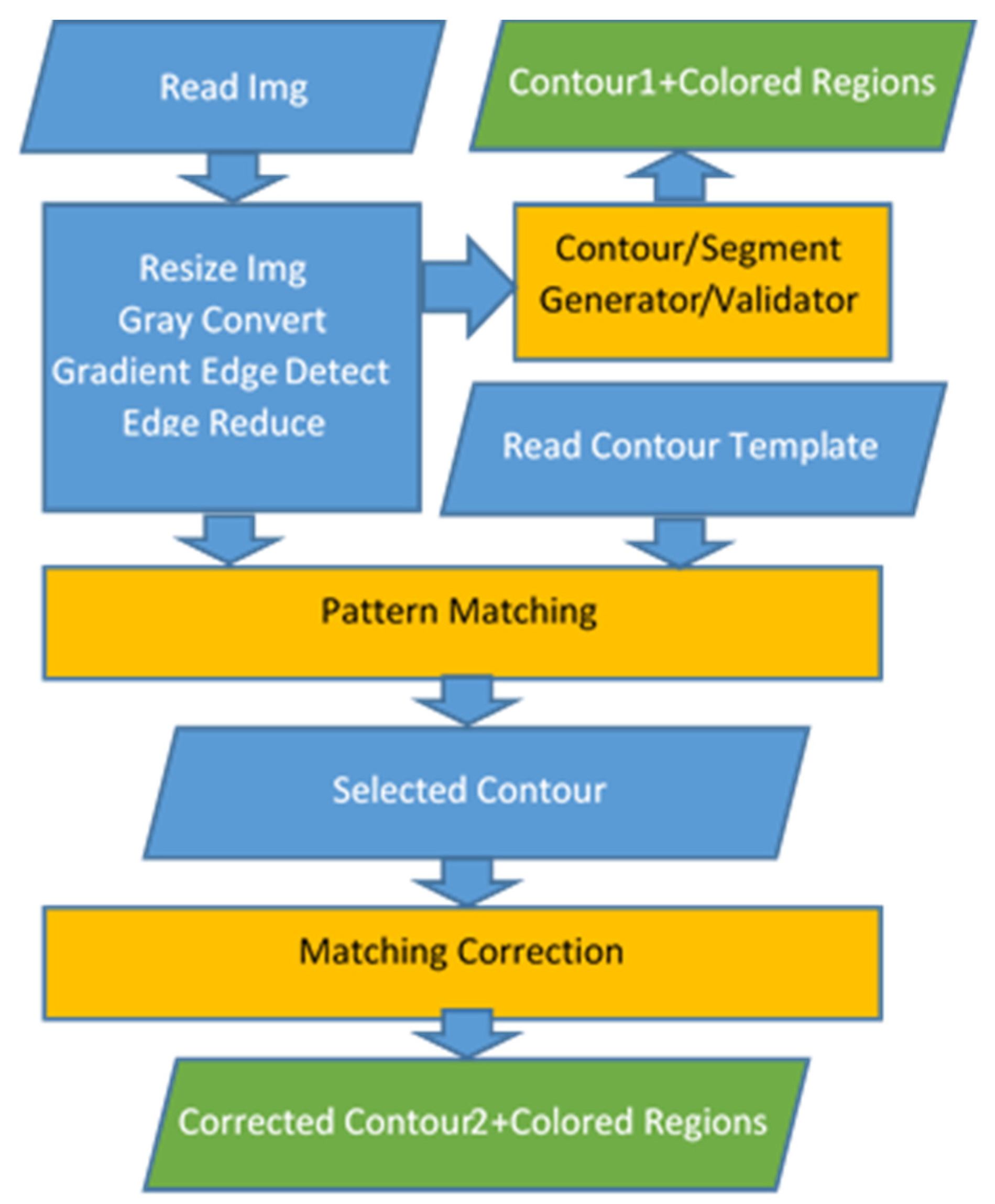
The first approach in the estimation of the fish’s morphological features was based on image processing techniques, and the steps of this technique are shown in Figure 1. Octave-forge Image package functions were used to read and write images and then resize and convert them into gray scale, rotate them and perform pattern matching. Most of the Octave Image package functions used were compatible with the corresponding OpenCV library routines; thus, portability to other platforms was guaranteed. As a first step, the initial image was read and resized to the supported resolution (80 rows, 160 columns). The specific resolution adaptation was necessary in order to avoid undesired overlapping with the patterns that would be tested for matching. The image was converted into gray scale for edge extraction.
The discontinuities of the image corresponded to the edges of the objects appearing in the image. We desired to select the edges that corresponded to the contour of the fish in order to match an appropriate pattern template. Both coarse algorithms, such as the Sobel algorithm [27] and more sensitive ones (e.g., Canny [28]) were tested. Canny is based on frame-level statistics, and it is more accurate than Sobel but has higher complexity and latency. Experimental results showed that a finer edge detection algorithm such as Canny confused the adopted pattern matching algorithm, which often selected the wrong patterns with the wrong size, rotation and orientation.
A custom edge detection algorithm that takes advantage of the “imgradient” function of the Octave-forge Image package was developed, offering higher accuracy than Sobel but not the confusing detail of Canny. It is described in Algorithm 1. The “imgradient” function returns the gradient magnitude and direction associated with each pixel (in the matrices gm and gd, respectively). If the gradient magnitude of a pixel exceeds a high threshold (magn_limit1), the pixel is assumed to belong to an edge; otherwise, a change in the vertical gradient direction is examined. If the gradient direction between adjacent vertical pixels seems to be reversed, and the gradient magnitude is above a second lower threshold, magn_limit2 (average magnitude ≪ magn_limit2 ≪ magn_limit1), then the pixel is assumed to belong to the horizontal part of the fish contour. Horizontal gradient direction changes are intentionally ignored in order to avoid the detection of edges belonging to different objects. Since we assumed that the fish was at a horizontal alignment or with a slight inclination and never vertical, the largest part of the fish contour could be detected in this way, avoiding the detection of other irrelevant edges. This procedure corresponds to the gradient edge detect step of Figure 1. Next, the mask displaying the detected edges (edgesgm) is scanned again to remove isolated or small groups of pixels (noise). This is the edge reduce step in Figure 1 that corresponds to step 18 of Algorithm 1.
| Algorithm 1 Custom edge detection algorithm |
|
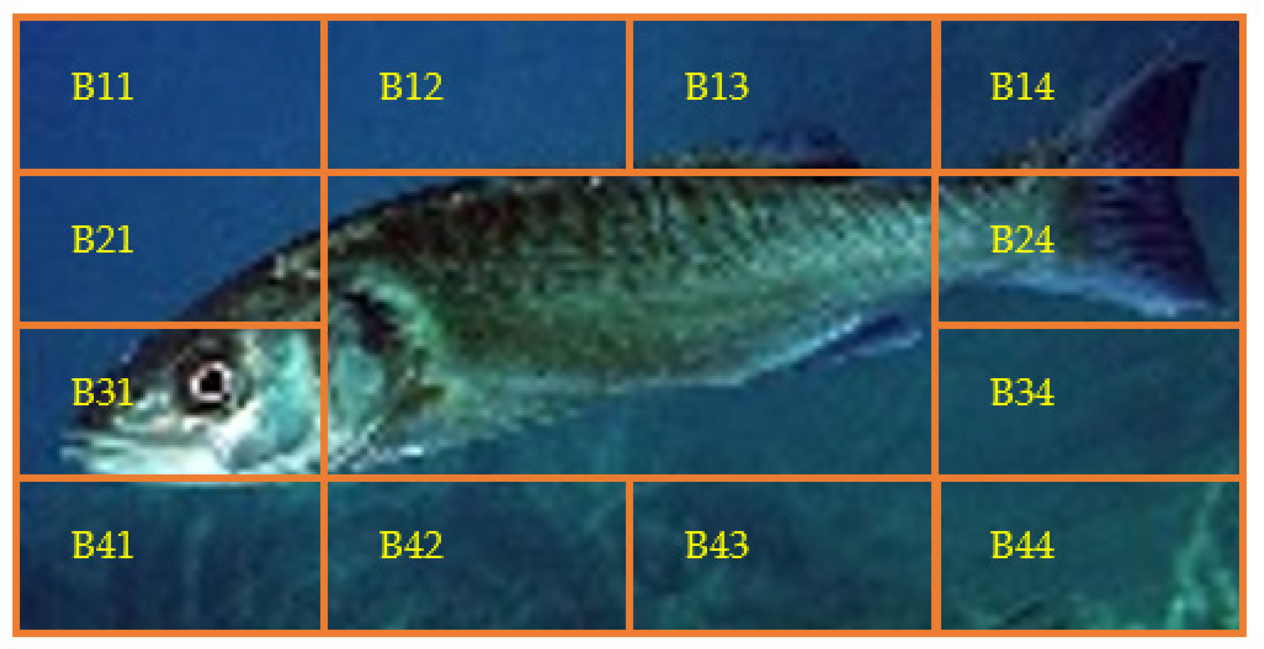
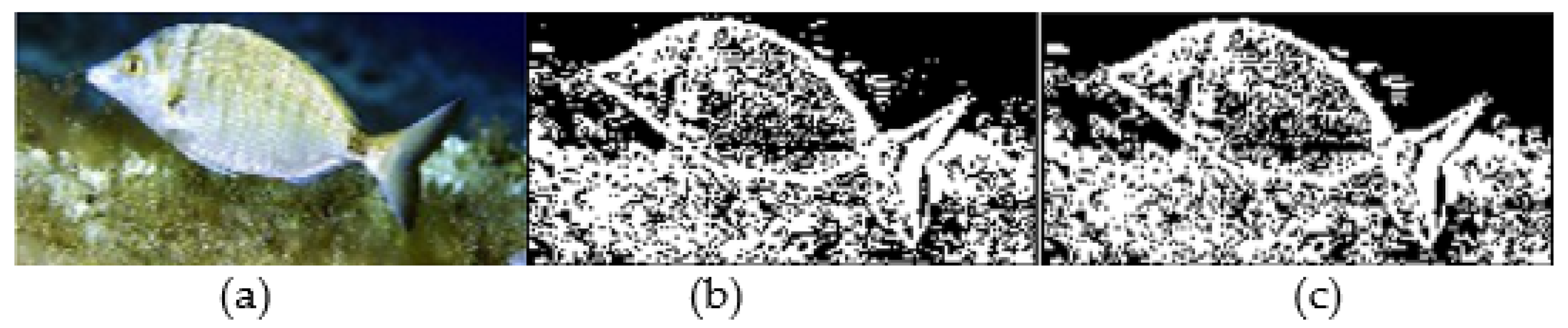
The first image processing approach toward the estimation of the fish contour and the localization of the fish parts exploits the edgesgm image produced after the edge detection step, as described in the previous paragraph. This approach is in the path that leads to the “Contour1” output in Figure 1. This path has low latency but produces valid results only if the background is simple (e.g., sea water). The system can validate whether this approach can be successfully followed using an image segmentation such as the one shown in Figure 2. Taking into consideration that the resolution of the resized images was 80 × 160 pixels, the size of each one of the segments shown in Figure 2, was 20 × 40 pixels. Assuming that the fish did not extend to the whole picture, it was expected that in most of the border segments B11-B21-B31-B41-B42-B43-B44-B34-B24-B14-B13-B12, the number of edges was small, unless the background was complex. The number of unconnected edges and the mean pixel value in each segment were estimated from the edgesgm matrix. Remember that a pixel in the edgesgm binary mask is one if it belongs to an edge, and it is 0 otherwise. If the number of disjointed edges in each segment was less than 10 and the mean pixel value in this segment was lower than 0.25, the segment was considered “empty” of edges; otherwise, it was characterized as “crowded”. An image displaying a fish with a simple background was expected to have a small number of crowded boundary segments, since only the boundary segments that contained a fish part would be crowded. If less than 6 segments were found to be crowded, the system assumed that the path toward “Contour1” in Figure 1 led to acceptable results. Figure 3 shows an example of an image that was rejected because 7 of the boundary segments were found to be crowded.
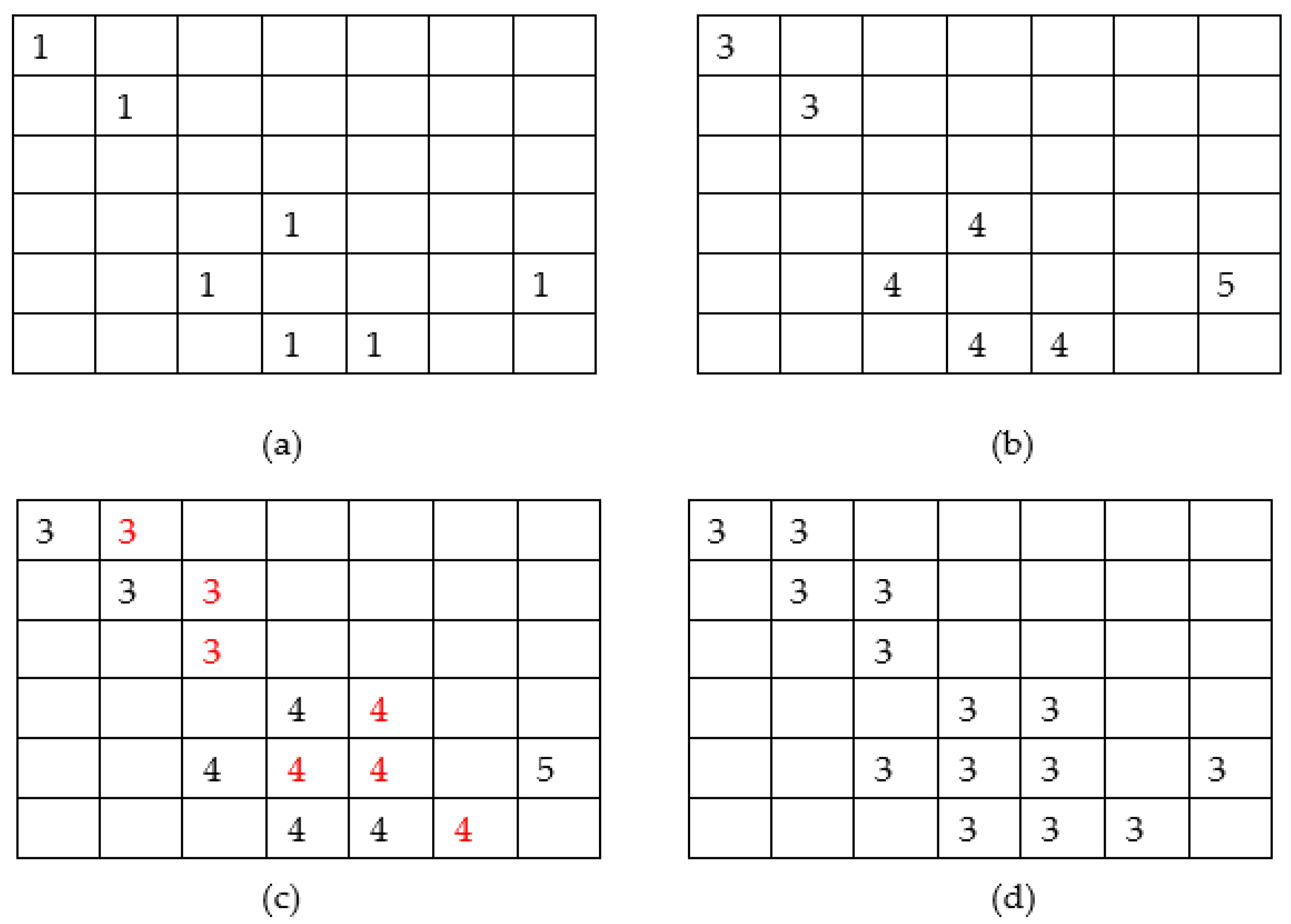
Once the system decides that the “Contour1” path in Figure 1 is not acceptable, it attempts to determine the fish contour based on the edges found in the matrix edgesgm. A connection of disjoint edges takes place as described in Figure 4. In Figure 4a, the contents of a part of the edgesgm binary mask are displayed, assuming that the ones belong to the fish contour. A second matrix edgesgm2 is constructed as follows. Each row (from top to the bottom) of edgesgm is scanned from left to right. An identity id is initialized to 0. All neighboring pixels are assigned with the same id. Figure 4b shows the form of edgesgm2 after its construction. In order to connect the disjoint edges, the matrices edgesgm and edgesgm2 are scanned again. If 1 is found in the pixel (i,j) of edgesgm, the corresponding pixel in the edgesgm2 matrix is set to id if one of the pixels (i − 1,j − 1), (i,j − 1) in edgesgm2 is already set to id. If none of these pixels have been set to a non-zero id, then the maximum value of id is increased by 1 and this value is assigned to edgesgm2(i,j). Figure 4c shows the matrix edgesgm2 after this step. As can be seen from this figure, the edges have been connected and thickened. To avoid having adjacent pixels with different identities in edgesgm2, a third scan takes place to merge neighboring identities (Figure 4d). After this merging process, the larger identity value corresponds to the number of disjoint edges. The larger edge (i.e., the one that contains the larger number of pixels) is selected as the contour of the bigger fish that is displayed in the photograph. In this way, although multiple fish can exist in the image, the analysis will proceed with the largest one. Complicated shapes in the body of the fish may confuse the proposed method. Consequently, a solid representation of the fish is generated by setting to 1 all the pixels within the (assumed) fish contour. The border of this solid fish body is now used as the fish contour in the pattern matching.
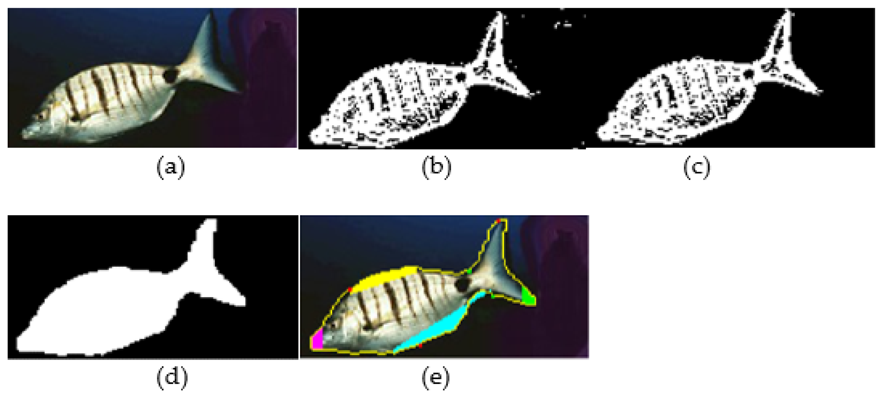
In order to determine the points that mark the borders of the fish parts, the fish contour is walked pixel by pixel, registering the corners (detected from direction changes) as landmarks. Using the morphology around the left and the right limits of the contour, the system recognizes the orientation of the fish. The location of the fish mouth can be easily determined in this case. On the opposite side, the area of the caudal fin is determined from the first corners of the upper and the lower part of the fish contour. For example, if the fish faces left, its mouth is at the point (i,j) on the contour with the lower j (pixel (0,0) is the upper left corner of the image). The line connecting the rightmost corners of the upper and lower part of the contour is used to delimit the caudal fin. The other corners of the upper and lower parts of the contour can be used to determine the position of the spiny or soft dorsal fins and the anal or pelvic fins, respectively. For example, three consequent corners may indicate the start, peak and the end of a fin. The line connecting the start and the end corner in conjunction with the fish contour delimit the fin. Figure 5 shows an example of a fish image processed with this approach. Figure 5a is the original photograph. When the edges are detected using Algorithm 1, the edgesegm matrix representation is shown in Figure 5b. Figure 5c shows the edgesegm matrix after the edge reduction step that removes small islands of edge pixels that are considered to be noise. In Figure 5d, the fish body was filled as explained earlier. Finally, in Figure 5e, the recognized fish parts are colored: the mouth with pink, the spiny and soft dorsal fins with yellow, the pelvic and anal fins with light blue and the caudal fin with green. As can be seen from Figure 5e, the caudal fin was partially recognized due to the orientation of the fish not allowing the proper determination of the upper corner.
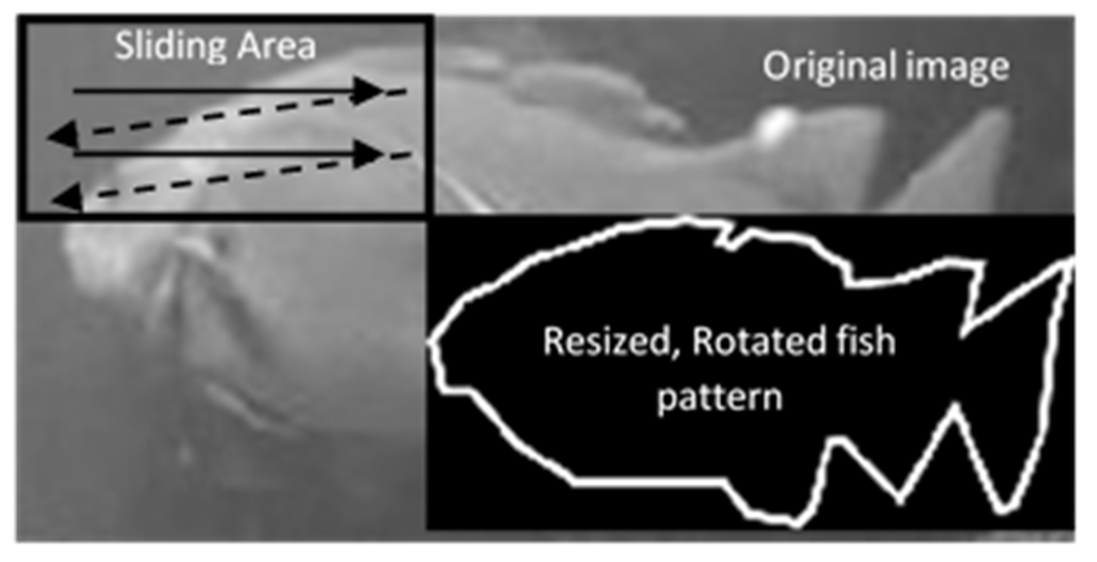
If the “Contour1” flow is unacceptable for a specific image, the pattern-matching path that leads to “Contour2” of the image processing approach can be followed. This method can be applied to images with more complicated backgrounds and attempts to match a contour pattern with the largest fish displayed. Algorithm 2 describes the Contour2 path, and it is used for every fish pattern ptrn that has to be tested. The external loops (lines 3 and 4 of Algorithm 2) modify the input ptrn by resizing (at line 7) and rotating it (at step 8) using the predefined strides sscl and sφ, respectively. Small strides can increase the accuracy, but they also increase the latency. The next step would be to slide the scaled and rotated fish pattern ptrn3 at the allowed positions of edgesgm as shown in Figure 6. In each position (r,c) of the ptrn3 within edgesgm, the correlation score Sc is estimated as
| Algorithm 2 Pattern matching algorithm for the Contour2 approach |
|
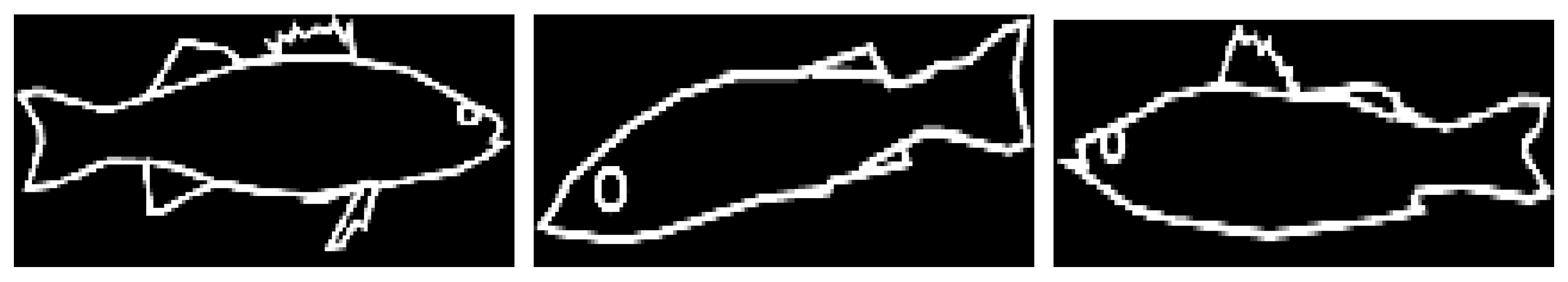
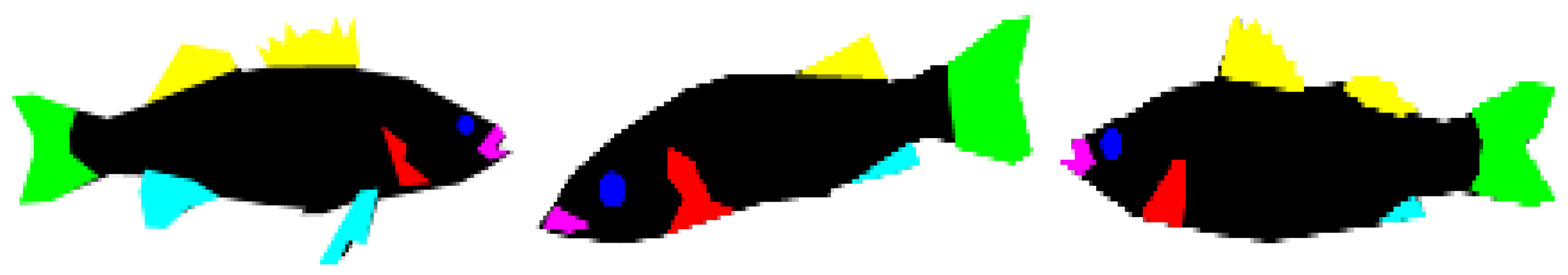
The configuration (parameters rot, scl, r and c) that achieved the best score were selected for the specific pattern ptrn. Sliding the resized and rotated pattern in successive (r,c) positions for the estimation of the correlation score using Equation (1) could be automatically performed with the normxcorr2 function in the Octave Image package (Algorithm 2). The same procedure was repeated for all the patterns of the specific fish species. If the fish species displayed in the tested image was not known a priori, all the supported patterns T had to be tested. In our case, where 25 images were used from each species, 3 patterns were representative for each species, and their horizontal mirror patterns were also used. For example, the 3 patterns used for sea bass are shown in Figure 7. The corresponding patterns with colored parts appear in Figure 8, since there was no need to use landmarks to delimit these parts in the Contour2 flow. As can be seen from Figure 7 and Figure 8, the set of fish patterns could be extended with already-rotated or slanted patterns (as is the one in the middle of Figure 7). The actual fish dimensions were already known for a specific pattern, scaling and rotation.
It is obvious that the latency of the Contour2 flow depends on the number of patterns and the different scaling and rotation values tested. The number of different Sc scores (Nt) that have to be estimated are
where Smax is the maximum scaling factor and the rotation angle of the pattern ranges between −φ and +φ, while strd and sφ are the scaling and angle stride, respectively.
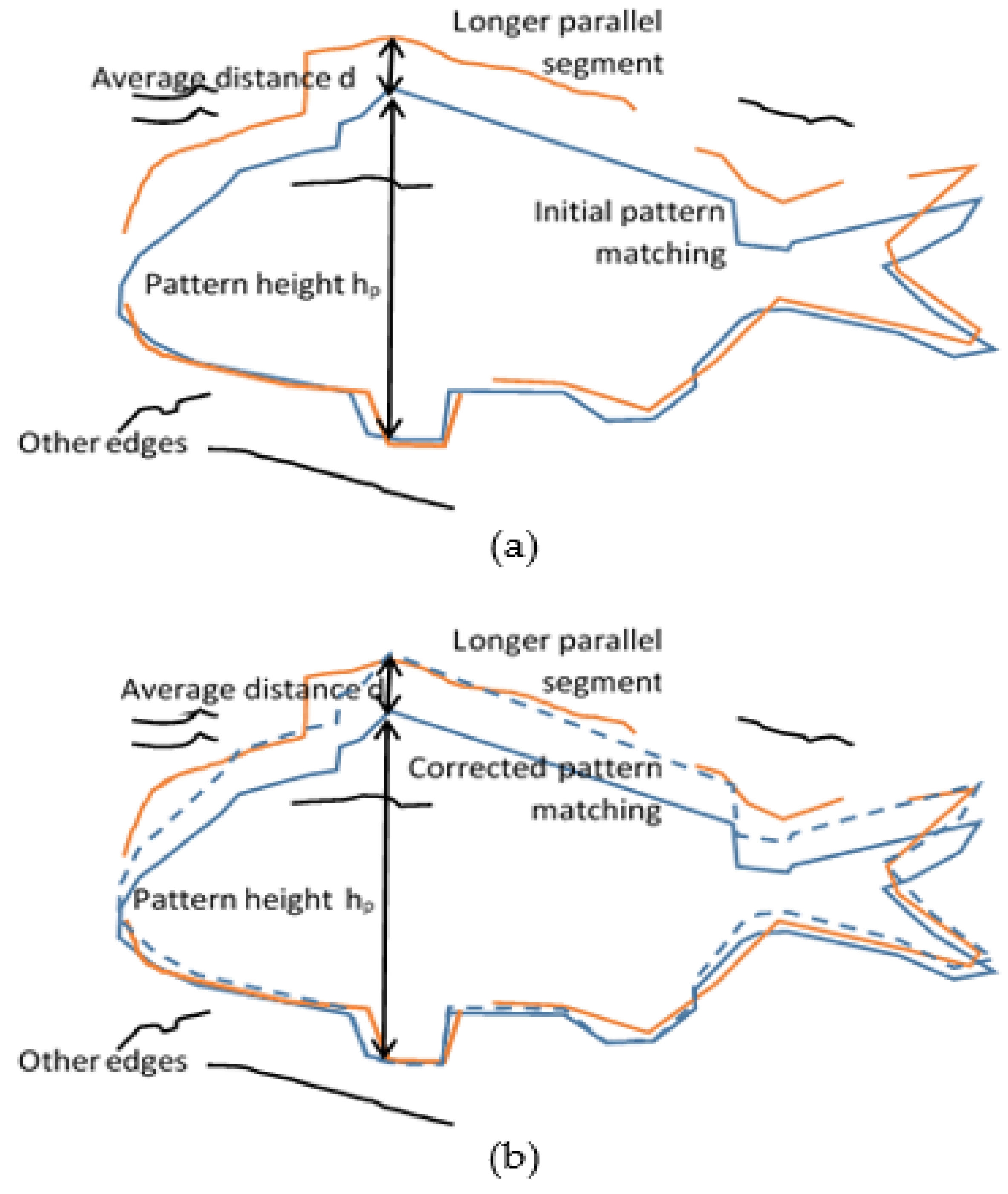
After the contour selection, the matching correction step shown in Figure 1 takes place. The matching correction procedure is described using the example of Figure 9, where the selected contour pattern (blue line) mainly matches the lower part of the fish (red edge segments). However, the resized pattern used failed to match the upper contour of the fish. The matching correction step examines the unmatched edge segments in the edgesgm mask in order to find the one with the maximum length that is parallel with a part of the pattern contour. The parallelism score in the vertical or horizontal direction Ps is defined as
Let us assume that an unmatched segment is examined for vertical parallelism with the contour, as is the case in Figure 9. The Euclidean distance |pk-ck| between each pixel pk of the unmatched segment and the pixel ck of the contour in the same column is estimated. The parallelism score Ps is the number of pixels that have a Euclidean distance within the range (d − ε, d + ε). In the same way, a segment can be examined for horizontal parallelism if pk and ck are in the same row. If a long edge segment has an acceptable Ps grade, the matching correction process will stretch the contour pattern in the corresponding direction to match this external segment. More specifically, in the case of Figure 9, if the height of the initial contour pattern is hp, and the average distance of the external edge segment is d, the contour pattern will be resized to an overall height equal to hp + d (Figure 9b). The corresponding fish pattern with colored parts (Figure 8) will also be resized in the same way to localize the fish parts more accurately without using landmarks in the way they were used in the Contour1 flow. However, corners and landmarks have to be determined for the estimation of the fish length and height. Examples of Contour2 flow output images are shown in Figure 10.
2.3. BMA and SCIA Deep Learning Approaches
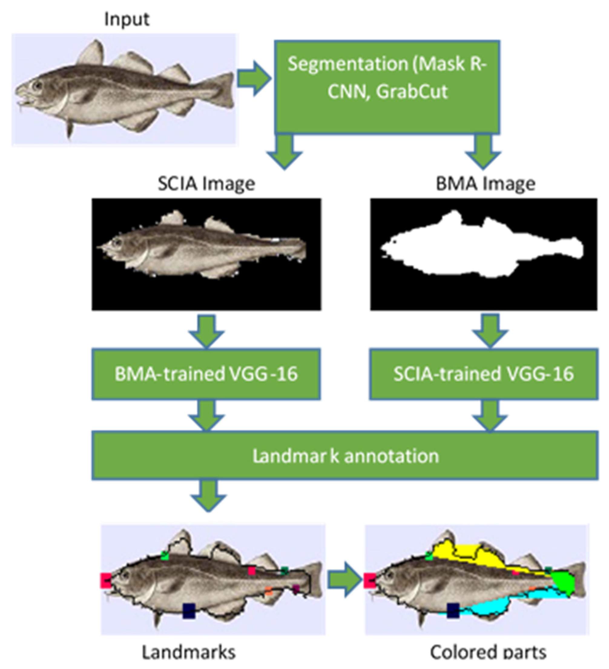
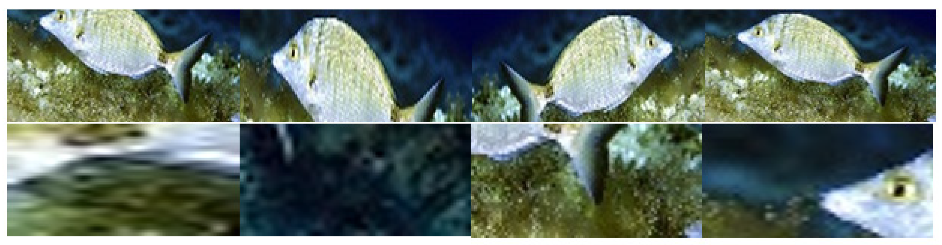
The steps followed in the deep learning approaches are shown in Figure 11. The input image is initially segmented based on the method described in [29]. The bounding box and the pixel-wise segmentation mask of all the recognized objects in the image are predicted using a mask region-based convolutional neural network (Mask R-CNN). It has to be noted that multiple objects can be recognized with different confidence levels. The largest fish will be recognized with higher confidence, while smaller or slanted or obscured fishes can also be recognized with lower confidence if the system is trained appropriately. In the current version, only the object with the highest confidence level is further processed. As was already mentioned in Section 2.1, the initial dataset consisting of 25 photographs or species is augmented by mirroring or cropping the initial images and applying jitter in order to generate multiple images from a single image. The resulting images are assumed to display a fish if less than 20% of the fish has been excluded from the cropped image (Figure 12). A higher threshold can be used if the obscured fish have to be recognized.
The Mask R-CNN was introduced in [30] as a successor of the Faster R-CNN. A binary mask output is added to the class name and bounding box output of the Faster R-CNN. The Mask R-CNN adds a fully connected CNN on top of the Faster R-CNN features. The backbone architectures employed in the Mask R-CNN are ResNet and ResNeXt of depths of 50 or 101 layers, respectively [30]. As shown in [29], the segmentation of the Mask R-CNN is not very precise, since regions that do not belong to the object are included in the output mask. Therefore, the GrabCut algorithm [24] was employed to improve the segmentation of the object that was recognized by the Mask R-CNN. However, GrabCut, in its attempt to exclude non-fish regions, may also exclude fish parts from the mask. None of the two approaches (individual Mask R-CNN or Mask R-CNN with GrabCut) can perform perfect contour detection. Therefore, OpenCV implementation of the GrabCut algorithm was used. The Mask R-CNN was pretrained with the COCO data set [31]. The COCO dataset contains 80 object categories and more than 120,000 images, but no fish species. However, it can segment fish objects in a satisfactory way, even if it does not recognize the displayed fishes. Alternative segmentation methods such as U-Net [32] could have been employed. U-Net can be trained on small data sets, and it is appealing for mobile implementations since it requires a small number of resources. Recent U-Net approaches [33,34,35] further improved the speed, the model and the training dataset size. U-Net has been tested mainly on medical imaging, and for this reason, a more general architecture (Mask R-CNN) was employed here.
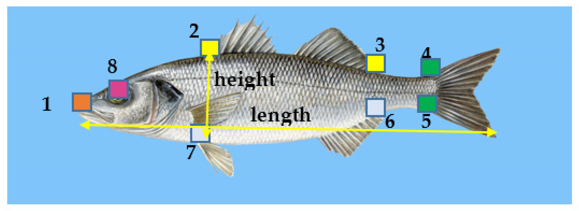
In the training procedure, 8 landmarks that were common to the four fish species studied here were annotated either on the binary mask (binary mask annotation (BMA)) or on the segmented colored image after subtracting the background (segmented color image annotation (SCIA)). The landmarks used in the deep learning approach are shown in Figure 13. Landmark 1 determined the position of the mouth. The pairs of landmarks (2,3), (4,5) and (6,7) determined the limits of the fins at the top (spiny and soft dorsal), the caudal fin and the fins at the bottom (anal and pelvic). Landmark 9 corresponded to the position of the eye, but it could not be determined accurately with the specific dataset size. The fish body height was defined as the Euclidean distance between landmarks 2 and 7. The fish body length was defined as the Euclidean distance between the mouth landmark (landmark 1) and the position of the farthest contour pixel on the opposite side (caudal fin).
New datasets were formed from the BMA or SCIA masks, along with the annotated landmarks. These datasets were used for the training of a VGG16 CNN using Keras and Tensorflow. The VGG16 CNN was trained to generate the 8 pairs of coordinates of the fish landmarks shown in Figure 13. The VGG16 CNN architecture that was already trained on ImageNet [25] was employed in the transfer learning method that followed. The fully connected head layer of the VGG16 model was removed. The weights in all other layers were frozen, and a new fully connected layer head was constructed with 8 pairs of landmark coordinates as the output. During the additional training process followed to train the new head layer, the estimated landmarks were compared with the ground truth landmarks annotated on the SCIA image. The weights of the new head layer were determined using mean squared error (MSE) loss and the Adam optimizer.
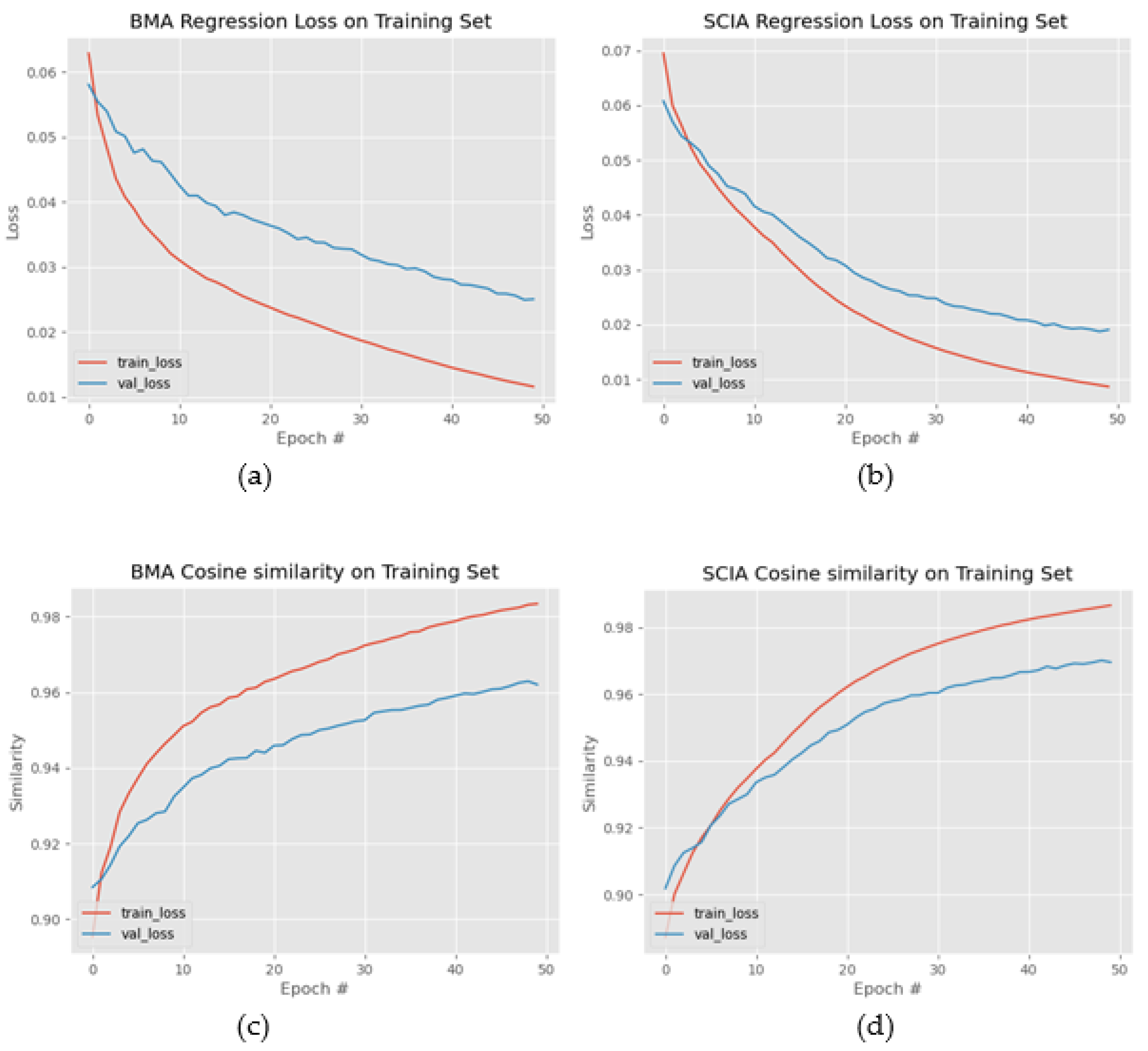
The regression loss of the training and the validation set for the BMA and the SCIA datasets are drawn in Figure 14a,b, respectively. Fifty (50) epochs were sufficient for flattening the regression loss curves; thus, the training could be terminated after 50 epochs for the specific dataset to avoid overfitting. The cosine similarity was also employed in Figure 14c,d in order to measure the alignment of the predicted positions with the true landmark positions. The cosine similarity of two non-zero vectors V1 and V2 was estimated as , where “·” denotes the dot product. Cosine similarity values +1, −1 and 0 corresponded to the fully aligned, opposite or orthogonal vectors, respectively.
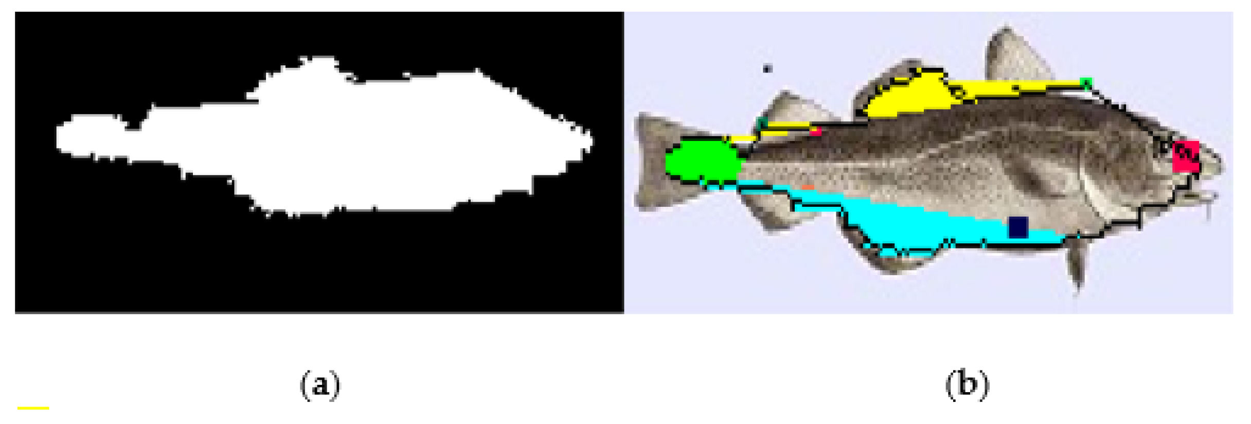
The VGG16 CNN was used for object detection and landmark annotation on a test image [32]. The fish contour was determined from the binary mask that was generated by the Mask R-CNN. The annotated landmarks were used to measure the fish dimensions (length and height) and to delimit the fish parts of interest (i.e., the caudal fin, the spiny and soft dorsal fins, the anal and pelvic fins and the mouth). The aforementioned procedure (training and testing) was implemented in Python. The distances were calculated, and the contour, the landmarks and the colored fish parts were available in the output image of this approach, as shown in Figure 15.
2.4. Estimation of Absolute Dimensions
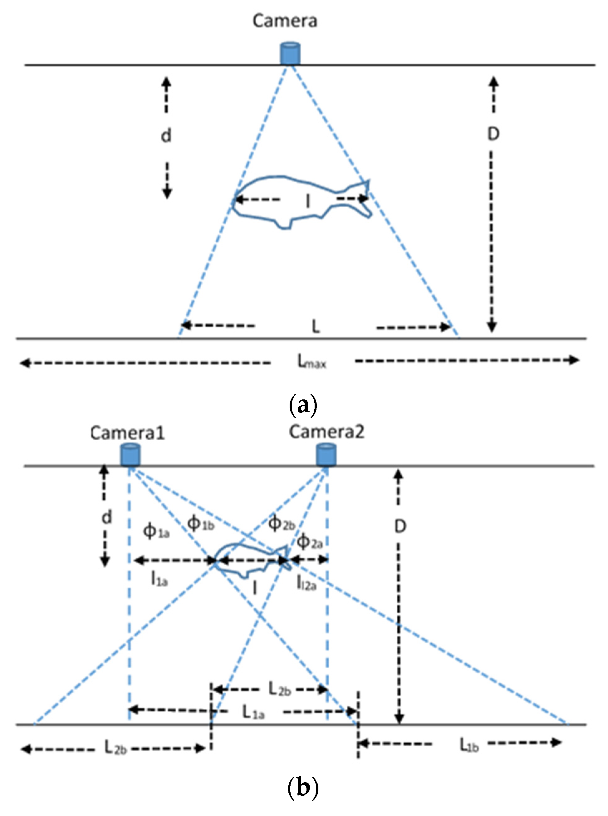
A single camera could not be used to estimate the absolute dimensions of a fish or any other object unless its distance from the object was known. In some cases, this is feasible (e.g., in intrusive methods that require the fish to be taken out of the tank and placed on a table in order to measure its length and weight). Instead of measuring these dimensions manually, a camera placed in a constant position and at a known distance from the fish could be used to estimate automatically the required features, as shown in Figure 16a. In this figure, the camera is facing a bench or a wall, which is denoted by the bottom horizontal line. Let us assume that the camera field of view can display the Lmax length of the bench and the corresponding number of pixels in this direction is Pmax. The distance of the camera from the bench is D. If the fish was at this exact distance from the camera, and its length L corresponded to P pixels, then
If the fish is at a known distance d, its actual length l can be scaled as follows:
This way of measuring the fish length could also be applied if the image was captured when the fish entered a narrow fishway, as described in [5]. If the fish distance was not known, then stereoscopic vision could be applied using a pair of cameras. In [6,16], popular methods based on epipolar planes were described for measuring absolute fish dimensions. Moreover, in [7], affine transformations were applied to adapt the shapes of fish that were photographed from an angle. A slightly different modeling than epipolar planes is described here. The modeling concerns the case where the fish is assumed to be parallel with the background wall or bench, and its length is measured at an unknown distance d as shown in Figure 16b.
From the view of each individual camera, the distances concerning the projection of the fish on the background bench (L1a, L1b, L2a, L2b) can be estimated using Equation (4). Knowing these parameters and the distance D of the cameras from the background wall, the angles φ1a, φ1b, φ2a and φ2b can be estimated as follows:
Now, assuming that the angles φ are already known, we also estimate the tangents at the distance d of the fish, and we also take into consideration that the distance LC from the cameras is known:
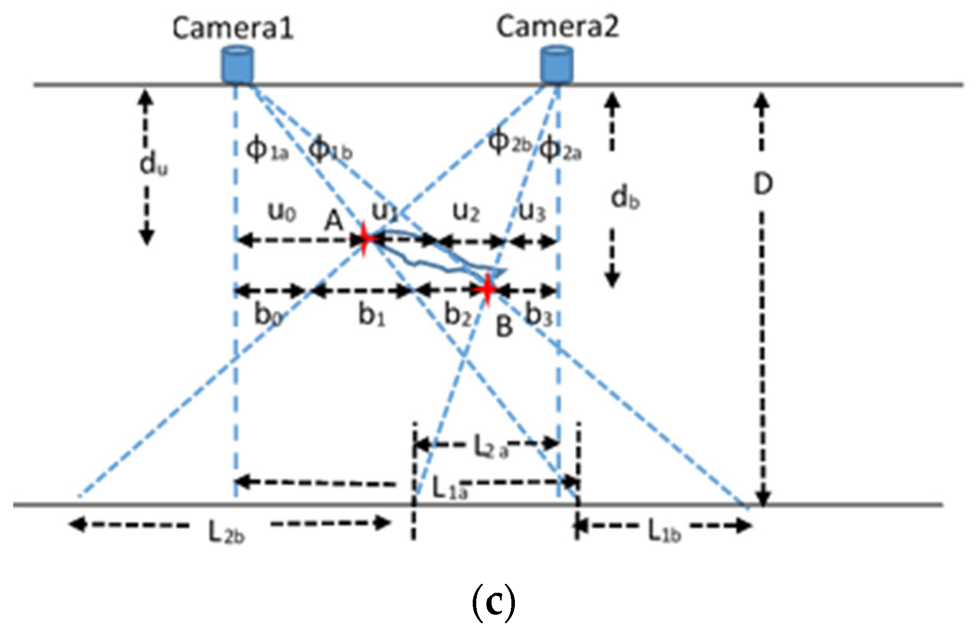
From Equations (10)–(14), the parameters d, l1a, l and l2a can be calculated. Using a similar approach, the length of a slanted fish can also be estimated as shown in Figure 16c. In this figure, the length of the fish is the Euclidean distance between points A and B. The positions of points A and B can be determined if the pairs of distances (du, u0) and (db, b3) are known, respectively. Assuming again that L1a, L1b, L2a and L2b have been estimated using Equation (4), the five pairs of equations that will lead to the determination of the positions of points A and B are the following:
3. Experimental Results—Discussion
The errors in the estimation of four parameters were examined first: length, height, area and area overlap. The error in the area was estimated from the comparison of the number of pixels enclosed by the fish contour, which was estimated by one of the methods presented in this paper, with the number of pixels enclosed by the actual fish contour. However, a different object may have been recognized as a fish with comparable dimensions. For this reason, area overlap error was also defined as the fraction of the actual fish pixels that did not overlap with the estimated fish area. The experimental results concerning these error parameters for the image processing techniques described in Figure 1 are presented in Table 1. The results listed in Table 1 concern either the Contour1 or Contour2 path, since the developed application could automatically select the appropriate results as described in Section 2.2. The estimated errors using the BMA and SCIA deep learning techniques described in Figure 11 are listed in Table 2 and Table 3, respectively.
The developed methods attempted to localize the following fish parts: the mouth and the spiny, dorsal, pelvic, anal and caudal fins. The image regions recognized to correspond to these parts were colored appropriately. Ideally, the recognized regions should match the actual fish part, but in practice, three cases were met: (1) the recognized region pixels were a subset of the corresponding fish part (partial match), (2) the recognized region was overlapping with the fish part (overlapping match) and (3) the recognized region was outside the fish part (matching failure). The purpose of the fish part recognition was to extract additional features concerning this specific region (e.g., dimensions, color and texture). Therefore, a partial match (if a full match is not possible) was preferable to an overlapping match, since in the case of overlapping, additional processing may be required. For example, the area that did not belong to the fish part could be excluded based on texture or geometrical restrictions. Table 4, Table 5 and Table 6 list the experimental results of the fish part localization for image processing and the deep learning BMA and SCIA methods, respectively. The recognition was considered successful if it was recognized with a full, partial or overlapping match.
From Table 1, Table 2, Table 3, Table 4, Table 5 and Table 6, it can be deducted that there was not a single method that achieved the highest accuracy in all cases. The fish dimensions were measured more accurately by the image processing techniques. These approaches could also localize the caudal fin with higher accuracy. The deep learning techniques, and especially the BMA trained method, could localize the spiny, soft dorsal, pelvic and anal fins as well as the mouth position with higher accuracy. It is possible to exploit all these techniques in order to achieve the highest accuracy. For example, the same image can be used as input for the Contour1 path and the BMA deep learning inference concurrently. If the image background is simple enough, and thus the results of the Contour1 path are acceptable, the deep learning approach can be canceled. If the results of the Contour1 path are unacceptable, the image processing Contour2 path can be followed, and the deep learning approach can be allowed to finish. The results of the two methods can then be compared and combined.
The latencies of the deep learning and image processing approaches examined in this paper are listed in Table 7. The measurements were performed on an Intel Core i5-9500 CPU @3.00 GHz 6-core processor with 16 GB of RAM. The latencies of the BMA and SCIA deep learning approaches are displayed in the second and the third columns. The second column lists the initialization latency that concerns the time needed to load the pretrained model. However, this was required only once and did not have to be repeated for every frame that was processed. The latency for processing one frame ranged from 2.716 to 5.112 s. A doubled delay is required by the Contour1 image processing technique. While the average latency of the deep learning approach was 3.58 s, the one for the Contour1 image processing technique was 7.83 s.
The latency of the Contour2 image processing described by Algorithm 2 depended mainly on four factors: the number of pattern templates compared (T), the maximum scaling of the template (Smax), the stride in the pattern scaling (Strd) and the number of pattern rotation angles (Nφ). The number of template matchings (Ntm) that have to be examined is expressed as
where Npos is the number of positions the template has to visit for a specific scaling. The larger the scaling, the larger the Npos value and the smaller the template dimensions will be. For example, if the current scaling is sc, then the pattern is resized to . The width is reduced by 2sc, since the default image width is twice its height (the resolution is 80 × 160). The sliding area of Figure 6 is . If we assume that the pattern template is moving in the sliding area with stride = 1 vertically and stride = 2 horizontally, then . The average pattern template dimension (i.e., its number of pixels Npxl) can be estimated as
As can be seen from Table 7, the number of pattern templates is T = 12 (3 templates for each species), and in all cases, the maximum scaling is Smax = 40. This means that the smallest pattern template has a resolution of pixels. In three of the four cases listed in Table 7, five pattern rotation angles were tested (Nφ = 5), ranging between −10° and +10° with an angle stride of 5°. In one case, 9 rotation angles were tested (Nφ = 5), ranging between −20° and +20° with an angle stride of 5°. The scaling stride Strd ranged from one to four. As can be seen from Table 7, the Contour2 flow was the slowest method, and its actual latency depended on the selected configuration.
The features of the methods employed in this work are summarized in Table 8. As was already described, the Contour1 path can lead to very accurate morphological feature measurement at a reasonable speed, provided that the image has a simple background. Fish rotation and slant corrections can be performed using the affine transformation, which leads to the higher fish dimensions. An obscured fish can be detected if its contour is the longest in the edgesgm image, but dimension estimation and fish part localization cannot be performed, since the shape will not be the expected one in this case (corners cannot be determined, as described in Section 2.2). Contour2’s path is much slower, and its latency depends on the number of patterns, rotations and scaling levels tested. The accuracy might be high if successful pattern matching is achieved, but it will be much worse if an inappropriate pattern, orientation or scaling is adopted. Extending the pattern set with fish patterns that have known rotations or slants or display obscured fishes can lead to more accurate measurements in these cases with the cost of higher latency. The deep learning inference (BMA, SCIA) had the shortest latency. The accuracy achieved depended on the training set size. The system could also be trained with different classes of obscured and slanted fishes. The classification performed along with image segmentation could be used to recognize obscured or slanted fishes, triggering the necessary corrections.
None of the tested methods are appropriate for real-time processing of video frames. However, the system is not intended to be used in such applications, because even if it were capable of processing 30 frames/s, the user would not be able to view the colored fish parts changing at this rate. On the contrary, capturing a single photograph of the fish may be adequate in order to estimate its mass, dimensions and health through the color or texture of its parts. The reported latencies in the referenced approaches are comparable with our case. More specifically, in the approaches of Rodriguez et al. [4,6], the time needed to process a single frame could be up to 12 s. The framework proposed in [18] placed 23 landmarks on 13,686 objects (zooids) detected in 1684 pictures of fossil bryozoans in 3.12 min using a personal computer.
Table 9 compares the experimental results of the current work with the ones achieved in the referenced approaches. The fish part localization performed in this work can be considered as a classification problem (image regions belong to a fish part or the background). Although there are some approaches that achieve lower size estimation errors ([16,18,20]) than the current work, they do not offer the same functionality (i.e., fish part localization). The classification accuracy is comparable with the referenced approaches, and as can be seen from Table 9, the referenced works that performed classification did not offer fish size estimation as in our case. It is expected that both the size error and classification accuracy of the proposed framework can be significantly improved if the deep learning approaches have the opportunity to be trained with larger datasets.
4. Conclusions
Morphological feature extraction was performed with image processing and deep learning noninvasive methods in this paper. The relative fish length, height and area were estimated, with an average length error estimation of 4.93%. Fish part localization was also supported, with a success rate higher than 91%. The processing time of a single frame required at least 2.7 s. The dataset consisted of 4 species with 25 photographs per species.
Future work will focus on training and testing deep learning approaches with fish species that have larger datasets available. Modified image processing and deep learning techniques will also be tested. Finally, the proposed implementations will be ported to mobile platforms.
Funding
This research received no external funding.
Institutional Review Board Statement
Not applicable. All photographs used in this work are publically available on the Internet.
Informed Consent Statement
Not applicable.
Data Availability Statement
The data presented in this study are available on request from the corresponding author. The data are not publicly available due to potential commercial exploitation.
Conflicts of Interest
The author declares no conflict of interest.
References
- Bhatnagar, A.; Devi, P. Water quality guidelines for the management of pond fish culture. Int. J. Environ. Sci. 2013, 3, 1980–2009. [Google Scholar]
- Periyadi, G.; Hapsari, I.; Wakid, Z.; Mudopar, S. IoT-based guppy fish farming monitoring and controlling system. Telkomnika Telecommun. Comput. Electron. Control 2020, 18, 1538–1545. [Google Scholar] [CrossRef]
- Ahmed, M.; Rahaman, M.O.; Rahman, M.; Abul Kashem, M. Analyzing the Quality of Water and Predicting the Suitability for Fish Farming based on IoT in the Context of Bangladesh. In Proceedings of the International Conference on Sustainable Technologies for Industry 4.0 (STI), Dhaka, Bangladesh, 24–25 December 2019; pp. 1–5. [Google Scholar] [CrossRef]
- Rodriguez, A.; Rabuñal, J.R.; Bermudez, M.; Puertas, J. Detection of Fishes in Turbulent Waters Based on Image Analysis. In Natural and Artificial Computation in Engineering and Medical Applications; Ferrández Vicente, J.M., Álvarez Sánchez, J.R., de la Paz López, F., Toledo Moreo, F.J., Eds.; Springer IWINAC 2013; Lecture Notes in Computer Science; Springer: Berlin/Heidelberg, Germany, 2013; Volume 7931. [Google Scholar] [CrossRef]
- Rico-Diaz, A.J.; Rodriguez, A.; Villares, D.; Rabuñal, J.R.; Puertas, J.; Pena, L. A Detection System for Vertical Slot Fishways Using Laser Technology and Computer Vision Techniques. In Advances in Computational Intelligence; Rojas, I., Joya, G., Catala, A., Eds.; Springer IWANN 2015; Lecture Notes in Computer Science; Springer: Berlin/Heidelberg, Germany, 2015; Volume 9094. [Google Scholar] [CrossRef]
- Rodriguez, A.; Rico-Diaz, A.J.; Rabuñal, J.R.; Puertas, J.; Pena, L. Fish Monitoring and Sizing Using Computer Vision. In Bioinspired Computation in Artificial Systems; Ferrández Vicente, J., Álvarez-Sánchez, J., de la Paz López, F., Toledo-Moreo, F., Adeli, H., Eds.; Springer IWINAC 2015; Lecture Notes in Computer Science; Springer: Berlin/Heidelberg, Germany, 2015; Volume 9108. [Google Scholar] [CrossRef]
- Spampinato, C.; Chen-Burger, Y.-H.; Nadarajan, G.; Fisher, R.B. Detecting, Tracking and Counting Fish in Low Quality Unconstrained Underwater Videos. In Proceedings of the 3rd Internatinal Conference on Computer Vision Theory and Applications (VISAPP), Funchal, Madeira, Portugal, 22–25 January 2008; Volume 2, pp. 514–519. Available online: http://www.inf.ed.ac.uk/publications/report/1272.html (accessed on 13 May 2021).
- Alsmadi, M.K.; Omar, K.B.; Noah, S.A.; Almarashdeh, I. Fish Recognition Based on Robust Features Extraction from Size and Shape Measurements Using Neural Network. J. Comput. Sci. 2010, 6, 1088–1094. [Google Scholar] [CrossRef] [Green Version]
- Alsmadi, M.; Tayfour, M.; Alkhasawneh, R.; Badawi, U.; Almarashdeh, I.; Haddad, F. Robust feature extraction methods for general fish classification. Int. J. Electr. Comput. Eng. 2019, 9, 5192–5204. [Google Scholar] [CrossRef]
- Shah, S.Z.H.; Rauf, H.T.; Ullah, M.I.; Khalid, M.S.; Farooq, M.; Fatima, M.; Bukhari, S.A.C. Fish-Pak: Fish species dataset from Pakistan for visual features based classification. Elsevier Data Brief 2019, 27, 104565. [Google Scholar] [CrossRef]
- Sarika, S.; Sreenarayanan, N.M.; Fepslin, A.M.; Suthendran, K. Under Water Fish Species Recognition. Int. J. Pure Appl. Math. 2018, 118, 357–361. [Google Scholar]
- Dawar, F.U.; Zuberi, A.; Azizullah, A.; Khattak, M.N.K. Effects of Cypermethrin on Survival, Morphological and Biochemical Aspects of rohu(Labeorohita) during Early Development. Chemosphere 2016, 144, 697–705. [Google Scholar] [CrossRef] [PubMed]
- Sengar, N.; Dutta, M.K.; Sarkar, B. Computer vision based technique for identification of fish quality after pesticide exposure. Int. J. Food Prop. 2017, 20 (Suppl. 2), 2192–2206. [Google Scholar] [CrossRef] [Green Version]
- Alaimahal, A.; Shruthi, S.; Vijayalakshmi, M.; Vimala, P. Detection of Fish Freshness Using Image Processing. Int. J. Eng. Res. Technol. 2017, 5, 1–5. [Google Scholar]
- Petrell, R.J.; Shi, X.; Ward, R.K.; Naiberg, A.; Savage, C.R. Determining size and swimming speed in cages and tanks using simple video techniques. Aquac. Eng. 1997, 16, 63–84. [Google Scholar] [CrossRef]
- Shi, C.; Wang, Q.; He, X.; Zhang, X.; Li, D. An automatic method of fish length estimation using underwater stereo system based on LabVIEW. Comput. Electron. Agric. 2020, 173, 105419. [Google Scholar] [CrossRef]
- Li, D.; Hao, Y.; Duan, Y. Nonintrusive methods for biomass estimation in aquaculture with emphasis on fish: A review. Rev. Aquacult. 2020, 12, 1390–1411. [Google Scholar] [CrossRef]
- Porto, A.; Voje, K.L. ML-morph: A fast, accurate and general approach for automated detection and landmarking of biological structures in images. Methods Ecol. Evol. 2020, 11, 500–512. [Google Scholar] [CrossRef] [Green Version]
- Dalal, N.; Triggs, B. Histograms of Oriented Gradients for Human Detection. In Proceedings of the International Conference on Computer Vision & Pattern Recognition (CVPR’05), San Diego, CA, USA, 20–26 June 2005; pp. 886–893. [Google Scholar] [CrossRef]
- Yu, C.; Fan, X.; Hu, Z.; Xia, X.; Zhao, Y.; Li, R.; Bai, Y. Segmentation and measurement scheme for fish morphological features based on Mask R-CNN. Inf. Process. Agric. 2020, 7, 523–534. [Google Scholar] [CrossRef]
- Girshick, R.; Donahue, J.; Darrell, T.; Malik, J. Rich feature hierarchies for accurate object detection and semantic segmentation. In Proceedings of the IEEE Computer Society Conference on Computer Vision and Pattern Recognition, Columbus, OH, USA, 23–28 June 2014; pp. 580–587. [Google Scholar]
- Liang, Z.W.; Shao, J.; Zhang, D.Y.; Gao, L.L. Small object detection using deep feature pyramid networks. In Proceedings of the 19th Pacific-Rim Conference on Multimedia, Hefei, China, 21–22 September 2018; pp. 554–564. [Google Scholar]
- Mbelwa, J.T.; Zhao, Q.J.; Lu, Y.; Wang, F.S.; Mbise, M. Visual tracking using objectness-bounding box regression and correlation filters. J. Electron. Imaging 2018, 27, 2. [Google Scholar]
- Rother, C.; Kolmogorov, V.; Blake, A. GrabCut: Interactive foreground extraction using iterated graph cuts. ACM Trans. Graph. 2004, 23, 309–314. [Google Scholar] [CrossRef]
- Russakovsky, O.; Deng, J.; Su, H.; Krause, J.; Satheesh, S.; Ma, S.; Huang, Z.; Karpathy, A.; Khosla, A.; Bernstein, M.; et al. ImageNet Large Scale Visual Recognition Challenge. Int. J. Comput. Vis. 2015, 115, 211–252. [Google Scholar] [CrossRef] [Green Version]
- Kaggle: Your Machine Learning and Data Science Community. Available online: https://www.kaggle.com/ (accessed on 10 April 2021).
- Sobel, Ι.; Feldman, G. A 3 × 3 Isotropic Gradient Operator for Image Processing. In Pattern Classification and Scene Analysis, 1st ed.; Duda, R., Hart, P., Eds.; John Wiley and Son: Hoboken, NJ, USA, 1973; pp. 271–272. [Google Scholar]
- Canny, J. A Computational Approach to Edge Detection. IEEE Trans. Pattern Anal. Mach. Intell. 1986, 8, 679–698. [Google Scholar] [CrossRef] [PubMed]
- Rosebrock, A. Image Segmentation with Mask R-CNN, GrabCut, and OpenCV, 28 September 2020. Available online: https://www.pyimagesearch.com/2020/09/28/image-segmentation-with-mask-r-cnn-grabcut-and-opencv/ (accessed on 10 April 2021).
- He, K.; Gkioxari, G.; Dollár, P.; Girshick, R. Mask R-CNN. In Proceedings of the IEEE International Conference on Computer Vision (ICCV), Venice, Italy, 22–29 October 2017; pp. 2980–2988. [Google Scholar] [CrossRef]
- COCO: Common Objects in Context. Available online: https://cocodataset.org/#home (accessed on 10 April 2021).
- Ronneberger, O.; Fischer, P.; Brox, T. U-Net: Convolutional Networks for Biomedical Image Segmentation. Form. Asp. Compon. Softw. 2015, 9351, 234–241. [Google Scholar]
- Gadosey, P.K.; Li, Y.; Adjei Agyekum, E.; Zhang, T.; Liu, Z.; Yamak, P.T.; Essaf, F. SD-UNet: Stripping Down U-Net for Segmentation of Biomedical Images on Platforms with Low Computational Budgets. Diagnostics 2020, 10, 110. [Google Scholar] [CrossRef] [Green Version]
- Tran, S.-T.; Cheng, C.-H.; Nguyen, T.-T.; Le, M.-H.; Liu, D.-G. TMD-Unet: Triple-Unet with Multi-Scale Input Features and Dense Skip Connection for Medical Image Segmentation. Healthcare 2021, 9, 54. [Google Scholar] [CrossRef]
- Jiao, L.; Huo, L.; Hu, C.; Tang, P. Refined UNet: UNet-Based Refinement Network for Cloud and Shadow Precise Segmentation. Remote Sens. 2020, 12, 2001. [Google Scholar] [CrossRef]
Figure 1.
The image processing flow.

Figure 2.
Segmentation for the validation of the “Contour1 + Colored Regions” path.

Figure 3.
Original image (a), the edgesgm matrix after gradient edge detection (b) and the edgesegm matrix after edge reduction (c). The path “Contour1” is not acceptable, since 7 of its boundary segments were found to be crowded.
Figure 3.
Original image (a), the edgesgm matrix after gradient edge detection (b) and the edgesegm matrix after edge reduction (c). The path “Contour1” is not acceptable, since 7 of its boundary segments were found to be crowded.

Figure 4.
Example of edge pixels (1’s) in the edgesgm matrix (a), the initial assignment of values (the numbers 3–5) in edgesgm2 (b), the connection of disjointed edges with the red-colored numbers being the ones added in this process (c) and the merging of identities in connected edges (d).
Figure 4.
Example of edge pixels (1’s) in the edgesgm matrix (a), the initial assignment of values (the numbers 3–5) in edgesgm2 (b), the connection of disjointed edges with the red-colored numbers being the ones added in this process (c) and the merging of identities in connected edges (d).

Figure 5.
Processing of a photograph with the Contour1 path, showing the original image (a), after gradient edge detection (b), after edge reduction (c), after creating the solid fish body (d) and after coloring the fish regions (e).
Figure 5.
Processing of a photograph with the Contour1 path, showing the original image (a), after gradient edge detection (b), after edge reduction (c), after creating the solid fish body (d) and after coloring the fish regions (e).

Figure 6.
Sliding a resized and rotated fish pattern in the original gray scale image.

Figure 7.
The three patterns used for sea bass.

Figure 8.
The fish patterns used for sea bass with colored parts.

Figure 9.
An initial contour pattern matching that is based mainly on the lower part of the contour (a) and the corrected contour pattern that has been stretched vertically to fit to the unmatched longer parallel segment on the top (b).
Figure 9.
An initial contour pattern matching that is based mainly on the lower part of the contour (a) and the corrected contour pattern that has been stretched vertically to fit to the unmatched longer parallel segment on the top (b).

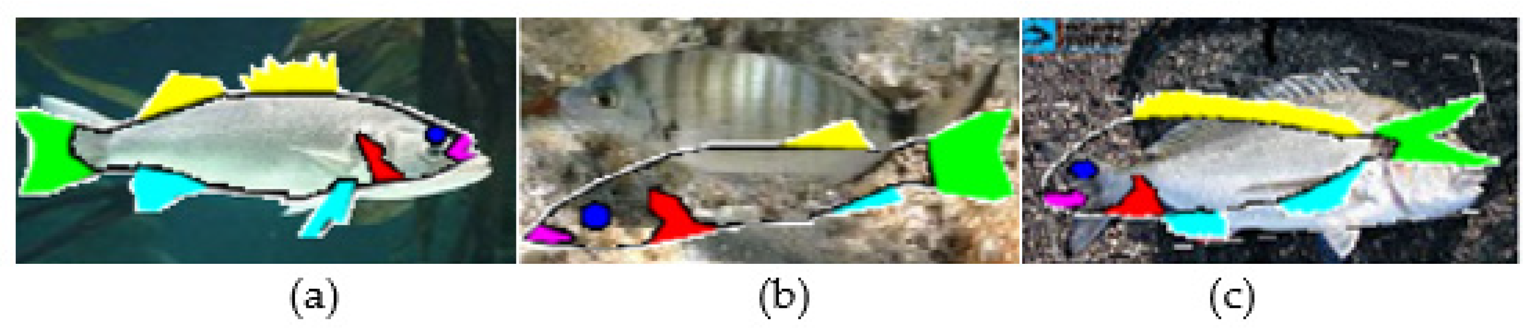
Figure 10.
Example output images from the Contour2 flow, showing an acceptable matching (a), matching error in the size and position (b) and matching error in the size, position and orientation (c).
Figure 10.
Example output images from the Contour2 flow, showing an acceptable matching (a), matching error in the size and position (b) and matching error in the size, position and orientation (c).

Figure 11.
The BMA and SCIA deep learning approaches.

Figure 12.
Augmenting the initial dataset, with the image variants that are recognized as displaying Figure 13. The landmarks are used in the deep learning approach.
Figure 12.
Augmenting the initial dataset, with the image variants that are recognized as displaying Figure 13. The landmarks are used in the deep learning approach.

Figure 13.
The landmarks used in the deep learning approach.

Figure 14.
Training and validation bounding box regression loss as a function of the number of epochs for BMA (a) and SCIA (b), with cosine similarity as a function of the number of epochs for BMA (c) and SCIA (d).
Figure 14.
Training and validation bounding box regression loss as a function of the number of epochs for BMA (a) and SCIA (b), with cosine similarity as a function of the number of epochs for BMA (c) and SCIA (d).

Figure 15.
An example of a BMA mask (a) and the input image with annotated landmarks and colored fish parts that is generated as the output of the deep learning approach (b).
Figure 15.
An example of a BMA mask (a) and the input image with annotated landmarks and colored fish parts that is generated as the output of the deep learning approach (b).

Figure 16.
Measuring the fish length from a known distance with a single camera (a), a fish that is not rotated and at an unknown distance with stereo vision (b) and a rotated fish at an unknown distance with stereo vision (c).
Figure 16.
Measuring the fish length from a known distance with a single camera (a), a fish that is not rotated and at an unknown distance with stereo vision (b) and a rotated fish at an unknown distance with stereo vision (c).


Table 1.
Dimension errors for the image processing approach of Figure 1.
Table 1.
Dimension errors for the image processing approach of Figure 1.
| Species | Area Error | Length Error | Height Error | Overlap Error |
|---|---|---|---|---|
| Dicentrarchus labrax | 27.8% | 6.6% | 9.1% | 10.3% |
| Diplodus puntazzo | 20.5% | 4.3% | 12% | 9.1% |
| Merluccius merluccius | 20% | 6.9% | 13% | 14.2% |
| Sparus aurata | 25% | 1.9% | 22.4% | 5.7% |
| Average | 23.33% | 4.93% | 14.13% | 9.83% |
Table 2.
Dimension errors for the deep learning BMA approach described in Figure 11.
Table 2.
Dimension errors for the deep learning BMA approach described in Figure 11.
| Species | Area Error | Length Error | Height Error | Overlap Error |
|---|---|---|---|---|
| Dicentrarchus labrax | 18.6% | 7.9% | 18.4% | 24.3% |
| Diplodus puntazzo | 26.4% | 15.6% | 15.5% | 24.9% |
| Merluccius merluccius | 22% | 12.2% | 11.7% | 25.8% |
| Sparus aurata | 24.4% | 12% | 15.5% | 26.5% |
| Average | 22.85% | 11.93% | 15.28% | 25.38% |
Table 3.
Dimension errors for the deep learning SCIA approach described in Figure 11.
Table 3.
Dimension errors for the deep learning SCIA approach described in Figure 11.
| Species | Area Error | Length Error | Height Error | Overlap Error |
|---|---|---|---|---|
| Dicentrarchus labrax | 18.5% | 9.6% | 20.3% | 25.5% |
| Diplodus puntazzo | 25.8% | 12.5% | 14.1% | 24.9% |
| Merluccius merluccius | 26.3% | 11.7% | 13.2% | 28.9% |
| Sparus aurata | 23.5% | 9.8% | 15.8% | 28% |
| Average | 23.53% | 10.90% | 15.85% | 26.83% |
Table 4.
Fish part localization for the image processing approach of Figure 1.
Table 4.
Fish part localization for the image processing approach of Figure 1.
| Species | Caudal | Spiny + Soft Dorsal | Pelvic + Anal | Mouth |
|---|---|---|---|---|
| Dicentrarchus labrax | 100.00% | 70.00% | 70.00% | 70.00% |
| Diplodus puntazzo | 90.00% | 56.30% | 61.10% | 80.00% |
| Merluccius merluccius | 80.00% | 65.00% | 75.00% | 30.00% |
| Sparus aurata | 100.00% | 60.00% | 31.30% | 50.00% |
| Average | 92.50% | 62.83% | 59.35% | 57.50% |
Table 5.
Fish part localization for the deep learning BMA approach described in Figure 11.
Table 5.
Fish part localization for the deep learning BMA approach described in Figure 11.
| Species | Caudal | Spiny + Soft Dorsal | Pelvic + Anal | Mouth |
|---|---|---|---|---|
| Dicentrarchus labrax | 80.0% | 100.0% | 90.0% | 95.0% |
| Diplodus puntazzo | 52.0% | 92.0% | 93.3% | 88.0% |
| Merluccius merluccius | 94.7% | 95.1% | 90.0% | 90.0% |
| Sparus aurata | 56.0% | 86.0% | 94.7% | 92.0% |
| Average | 70.68% | 93.28% | 92.00% | 91.25% |
Table 6.
Fish part localization for the deep learning SCIA approach described in Figure 11.
Table 6.
Fish part localization for the deep learning SCIA approach described in Figure 11.
| Species | Caudal | Spiny + Soft Dorsal | Pelvic + Anal | Mouth |
|---|---|---|---|---|
| Dicentrarchus labrax | 80.0% | 97.5% | 90.0% | 100.0% |
| Diplodus puntazzo | 50.0% | 91.7% | 89.3% | 66.7% |
| Merluccius merluccius | 94.7% | 89.5% | 55.3% | 84.2% |
| Sparus aurata | 73.1% | 76.4% | 97.6% | 66.7% |
| Average | 74.45% | 88.78% | 83.05% | 79.40% |
Table 7.
Latency of the fish morphological feature measurement approaches (in seconds).
| Deep Learing | Contour1 | Contour2 (Smax = 40, Tmpl = 12) | |||
|---|---|---|---|---|---|
| Initialization | Frame Processing | 534 | (Strd = 1, Nφ = 5) | ||
| Min | 1.325 | 2.716 | 5.835 | 128 | (Strd = 2, Nφ = 5) |
| Max | 1.552 | 5.112 | 10.41 | 53 | (Strd = 4, Nφ = 9) |
| Average | 1.364625 | 3.5835 | 7.831875 | 29 | (Strd = 4, Nφ = 5) |
Table 8.
Summary of employed method features.
| Method | Speed | Precision | Prerequisites | Supported Extensions or Corrections |
|---|---|---|---|---|
| Contour1 (image proc.) | Medium | High | Simple background | - Rotation or slant correction through optimized affine transformation |
| Contour2 (image proc.) | Low | Variant | Appropriate set of patterns | - Inherent rotation or slant correction - Detection of obscured fish |
| BMA and SCIA (Deep Learning) | High | Depends on the training dataset size | Appropriate annotations | - Selectable correction methods if fish is classified as rotated, slanted or obscured |
Table 9.
Comparison with the referenced approaches.
| Ref. | Size Error | Classification Accuracy | Species or Fish Families | Notes |
|---|---|---|---|---|
| [6] | 7–12% | |||
| [8] | 91–94% | 20 | Dataset = 350 fish images (93 for testing) | |
| [9] | 82–90% | 24 | Dataset = 250 training, 150 test images | |
| [13] | 92–97% | Treated or Untreated | ||
| [14] | 90% | |||
| [15] | ±9.5% | In 85%, the mass error is <6% | ||
| [16] | 2.55% | Relative error | ||
| [17] | 1–13% | |||
| [18] | Fish length error <1% | 3 zooid species | 13,686 zooids detected in 1684 pictures, 80% training, 20% test | |
| [20] | <3% | Relative error | ||
| This work | 4.93% (average) | >91% | 4 species | Size error is relative length, while classification accuracy refers to fish part localization |
Publisher’s Note: MDPI stays neutral with regard to jurisdictional claims in published maps and institutional affiliations. |
© 2021 by the author. Licensee MDPI, Basel, Switzerland. This article is an open access article distributed under the terms and conditions of the Creative Commons Attribution (CC BY) license (https://creativecommons.org/licenses/by/4.0/).
Share and Cite
MDPI and ACS Style
Petrellis, N. Measurement of Fish Morphological Features through Image Processing and Deep Learning Techniques. Appl. Sci. 2021, 11, 4416. https://doi.org/10.3390/app11104416
AMA Style
Petrellis N. Measurement of Fish Morphological Features through Image Processing and Deep Learning Techniques. Applied Sciences. 2021; 11(10):4416. https://doi.org/10.3390/app11104416
Chicago/Turabian StylePetrellis, Nikos. 2021. "Measurement of Fish Morphological Features through Image Processing and Deep Learning Techniques" Applied Sciences 11, no. 10: 4416. https://doi.org/10.3390/app11104416
Note that from the first issue of 2016, this journal uses article numbers instead of page numbers. See further details here.