An Improved Attention-Based Integrated Deep Neural Network for PM_2.5 Concentration Prediction

Abstract

The air quality prediction is a very important and challenging task, especially PM${}_{2.5}$ (particles with diameter less than 2.5 μm) concentration prediction. To improve the accuracy of the PM${}_{2.5}$ concentration prediction, an improved integrated deep neural network method based on attention mechanism is proposed in this paper. Firstly, the influence of exogenous series of other sites on the central site is considered to determine the best relevant site. Secondly, the data of all relevant sites are input into the improved dual-stage two-phase (DSTP) model, then the PM${}_{2.5}$ prediction result of each site is obtained. Finally, with the PM${}_{2.5}$ prediction result of each site, the attention-based layer predicts the PM${}_{2.5}$ concentration at the central site. The experimental results show that the proposed model is superior to most of the latest models.

1. Introduction

With the development of the economy, air pollution has become more and more serious, and has caused great harm to the health of urban residents [1]. Air quality prediction is a very important task in air pollution control. The existing research methods of air prediction are mainly divided into two kinds—deterministic methods and statistical methods. The deterministic method predicts air quality by building a simulation model of the diffusion and transport of atmospheric chemicals, such as the community multi-scale air quality model (CMAQ) [2,3,4] and the nested air quality prediction model system (NAQPMS) [5,6,7]. This kind of theory model needs a lot of prior knowledge and a large number of accurate data. There are many parameters in these theory models, which are difficult to set. Statistical prediction methods can overcome the limitations of deterministic methods by a large amount of data, such as linear regression [8,9] and multiple linear regression (MLR) [10,11,12]. However, the early linear models mentioned above assume that the relationship between variables and target labels is linear and is not applicable to nonlinear and unstable air quality prediction problems. In addition, traditional regression prediction models often fail to integrate and analyze multi-source heterogeneous data [13].

To solve the problems of the traditional air quality prediction models, more and more artificial intelligence models are proposed, which are based on machine learning. For example, Wang et al. [14] proposed a hybrid support vector machine (SVM) based prediction system, which is applied to the historical data of meteorological variables. Alimissis et al. [15] used an artificial neural network (ANN) to simulate the spatial variability of air pollution, which is better than MLR model in air pollution prediction. Zhu et al. [16] proposed two hybrid models (EMD-SVR-Hybrid and EMD-IMFs-Hybrid) to predict air quality data. These models have obtained some good results in air quality prediction. However, these models are all shallow neural networks. The computational units of the models are few, and the ability to express complex functions is limited. The generalization ability for complex prediction problems is limited.

Recently, a deep learning method has been widely used for air quality prediction and many research results have been presented [17,18]. For example, Kim et al. [19] used a recurrent neural network (RNN) model to predict the concentration of air pollutants on subway platforms. Zhao et al. [20] used the long short-term memory-fully connected (LSTM-FC) neural network to extract spatio-temporal characteristics from historical air quality and meteorological data of the target and neighboring sites, where only the fully connected layer is used as the spatial combinator, ignoring the PM${}_{2.5}$ concentration correlation between neighboring sites and the central site. Qin et al. [21] presented a combined prediction scheme based on convolutional neural network (CNN) and long short-term memory (LSTM), where CNN is used to compress input data to eliminate redundancy, the spatial correlation between data is determined, and the temporal dependence between pollutants is studied by LSTM. In this scheme, the accuracy of the model will be negatively affected by unrelated sites when data from all neighboring sites are entered into the model, and all input features are treated equally and cannot focus on the important features. Qin et al. [22] proposed a dual-stage attention-based recurrent neural network (DA-RNN), where the attention mechanism is not only in the input stage of the decoder, but also in the encoder stage so that the most relevant input features can be adaptively selected. However, in this method, a single-layer attention module is used in the encoder stage, and the weight learned is decentralized, which means this method is not effective for long term prediction. To deal with the shortcomings of the method in [22], Liu et al. [23] proposed a dual-stage two-phase attention-based recurrent neural network (DSTP-RNN), where the two-phase attention mechanism is adopted in the encoder stage, and the stable attention weight can be obtained. However, only one site’s data are used in this method, without considering the impact of other sites’ data on the model.

To deal with the problems in the deep learning based models introduced above and to further improve the effectiveness and accuracy of air quality prediction, an improved attention-based integrated deep neural network method is proposed, which is used to predict the PM${}_{2.5}$ (particles with diameter less than 2.5 μm) concentration. In this proposed method, an exogenous series correlation method is used to compute the relationship between the target series and the exogenous series, and the PM${}_{2.5}$ concentration is predicted in the improved dual-stage two-phase (DSTP) model.

The main contributions of this paper are summarized as follows: (1) The relationships between the target series of the central site and the exogenous series of other sites are considered in the PM${}_{2.5}$ concentration prediction, by using an exogenous series correlation method; (2) The DSTP model is improved to predict the PM${}_{2.5}$ concentration in the central site and the neighboring sites; (3) An attention-based fully connected layer is used to predict the final PM${}_{2.5}$ concentration of the central site. Finally, some experiments are conducted on the datasets of the air quality sites in Beijing. In addition, the performance of the proposed method is discussed and compared with other deep learning based methods. The results show the efficiency of the proposed method.

This paper is organized as follows—in Section 2, the proposed integrated deep neural network method is presented in details. Section 3 introduces the experiments of the proposed method in the PM${}_{2.5}$ concentration prediction on the real datasets of Beijing. Section 4 discusses the parameter setting and performance of the proposed method by some further experiments. Finally, conclusions and future work are given out in Section 5.

2. Proposed Method

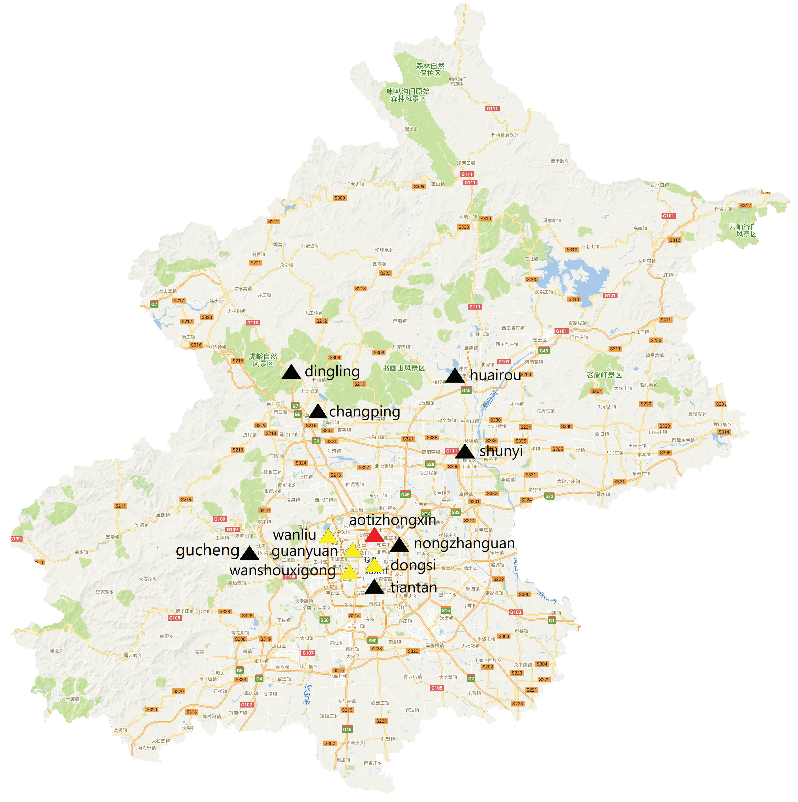
In order to improve the accuracy of PM${}_{2.5}$ concentration prediction, an improved attention based dual-stage two-phase fully connected (DSTP-FC) model is proposed in this paper, which is used for central site PM${}_{2.5}$ concentration prediction, and multi-site data are used as an input to help more accurately predict PM${}_{2.5}$ concentration at a central site. The data of twelve air quality sites in Beijing, China are used to test the proposed model, which will be introduced in detail in Section 3.1. The locations of these twelve air quality sites are shown in Figure 1, where the location of the central site is represented by a red triangle in the figure.

The inputs of the model include historical air quality and meteorological data. The data flow of the proposed method is shown in Algorithm 1.

Firstly, the spatiotemporal correlations between the central site and the neighboring sites are analyzed, according to the correlations of the target series in two sites (that is PM${}_{2.5}$ series), then the central site collection is set up. The locations of the neighboring sites are represented by yellow triangles in Figure 1.

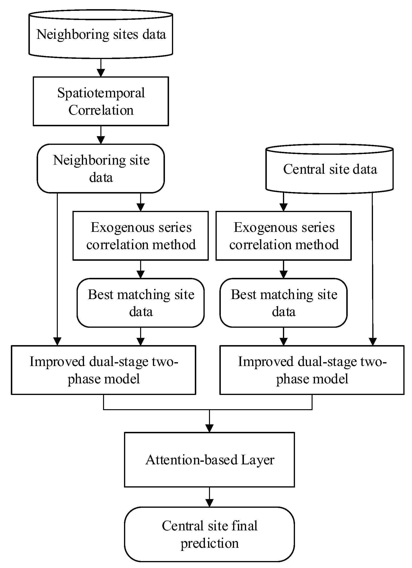
Secondly, the model selects one site with the highest correlation for all the sites in the central site collection from all other sites, according to the exogenous series correlation. Then the site pairs are obtained. The PM${}_{2.5}$ prediction results of each site pair can be obtained by inputting all data of these site pairs into the improved dual-stage two-phase model based on the attention mechanism, respectively.

Finally, the prediction results of all sites in these site pairs are input into the attention-based layer to get the prediction results of the central site.

The framework of the proposed method is shown in Figure 2 and is described in detail below.

Algorithm 1 The data flow of the proposed method

Input: All sites’ data for current batch, denoted as $P_n$;

Output: The prediction result of the central site $N_0$, denoted as S;

(1) Firstly, according to the target series of the central site and other sites, determine the relevant sites of the central site $N_0$. Here are $N_1$, $N_2$, $N_3$, $N_4$. These five sites are called the central site collection; (2) Secondly, according to the exogenous series of the sites in the central site collection and other sites, the matching sites are determined by the exogenous series correlation method. Here are $N_{best0}$, $N_{best1}$, $N_{best2}$, $N_{best3}$, $N_{best4}$ respectively; (3) Thirdly, the site pairs ($N_0$, $N_{best0}$), ($N_1$, $N_{best1}$), ($N_2$, $N_{best2}$), ($N_3$, $N_{best3}$), ($N_4$, $N_{best4}$) are input into the model respectively to get the prediction results of the sites in the central site collection. The site pair ($N_i$, $N_{bes{t}_i}$) contains the exogenous series and target series of these two sites. (4) Finally, with the prediction results of each site in the central site collection, the attention-based layer get the prediction result S of the central site;

returnS;

2.1. Spatiotemporal Correlation Analysis

Air pollutants are distributed at each site. Due to the wind influence, the air pollutants of one site will be affected by the neighboring sites air pollutants. Therefore, PM${}_{2.5}$ concentration should be predicted according to the air pollutants at the central site and the air pollutants at neighboring sites.

In this study, the Pearson correlation coefficient [24] is used to measure the spatial correlation of PM${}_{2.5}$ concentrations at all sites. Then, the autocorrelation function [25] is used to measure the temporal correlation between PM${}_{2.5}$ concentration series at each site. The calculation formulas are as follows:

$$r(s_i,s_j)=\frac{Cov(s_i,s_j)}{\sigma \left(s_i\right)\sigma \left(s_j\right)}$$

(1)

$${\rho }_k=\frac{Cov\left(y\right(t),y(t+k\left)\right)}{{\sigma }_{y\left(t\right)}{\sigma }_{y(t+k)}},$$

(2)

where $r(·)$ represents Pearson correlation coefficient between sites; ${\rho }_k$ represents autocorrelation coefficient at t and $t+k$ time within the same site; $y\left(t\right)$ and $y(t+k)$ respectively represent the air pollutants concentration at time t and $t+k$; $Cov(·)$ is the covariance; and $\sigma (·)$ is the standard deviation.

2.2. Improved Dual-Stage Two-Phase Model Based on Attention Mechanism

2.2.1. Notation and Problem Statement

(1) Notation

Assume that there are N sites for all sites, given all sites’ data, each site contains n exogenous series and a target series.

Within the window size T of the all sites, the k-th $(k⩽n)$ exogenous series is represented by

$$x^k={(x_1^k,x_2^k,\cdots ,x_T^k)}^T\in R^T.$$

(3)

All exogenous series is represented by

$$X={(x_1,x_2,\cdots ,x_T)}^T\in R^{n\times T}(x_k=x^k).$$

(4)

The target series is represented by

$$Y={(y_1,y_2,\cdots ,y_T)}^T\in R^T.$$

(5)

Then a concatenation of target series and the output of the first phase attention can be represented by

$$Z={(z_1,z_2,\cdots ,z_T)}^T\in R^{(n+1)\times T}.$$

(6)

Then, the future value of the target series can be represented by

$$\widehat{Y}={(y_{T+1},y_{T+2},\cdots ,y_{T+\tau })}^T\in R^{\tau },$$

(7)

where $\tau$ is the time step to be predicted.

(2) Problem statement

Given the exogenous series and target series of all sites, the exogenous series and target series of the e-th site in all sites are

$$(x_1^{\left(e\right)},x_2^{\left(e\right)},\cdots ,x_T^{\left(e\right)}),x_t^{\left(e\right)}\in R^n$$

(8)

and

$$(y_1^{\left(e\right)},y_2^{\left(e\right)},\cdots ,y_T^{\left(e\right)}),y_t^{\left(e\right)}\in R.$$

(9)

The model aims to predict the value of $\tau$ time steps in the future, which can be expressed as:

$$y_{T+1},y_{T+2},\cdots ,y_{T+\tau }=F(y_1^{\left(e\right)},\cdots ,y_T^{\left(e\right)},x_1^{\left(e\right)},\cdots ,x_T^{\left(e\right)}),e⩽N$$

(10)

where $F(·)$ is the nonlinear function to be learned.

2.2.2. Models

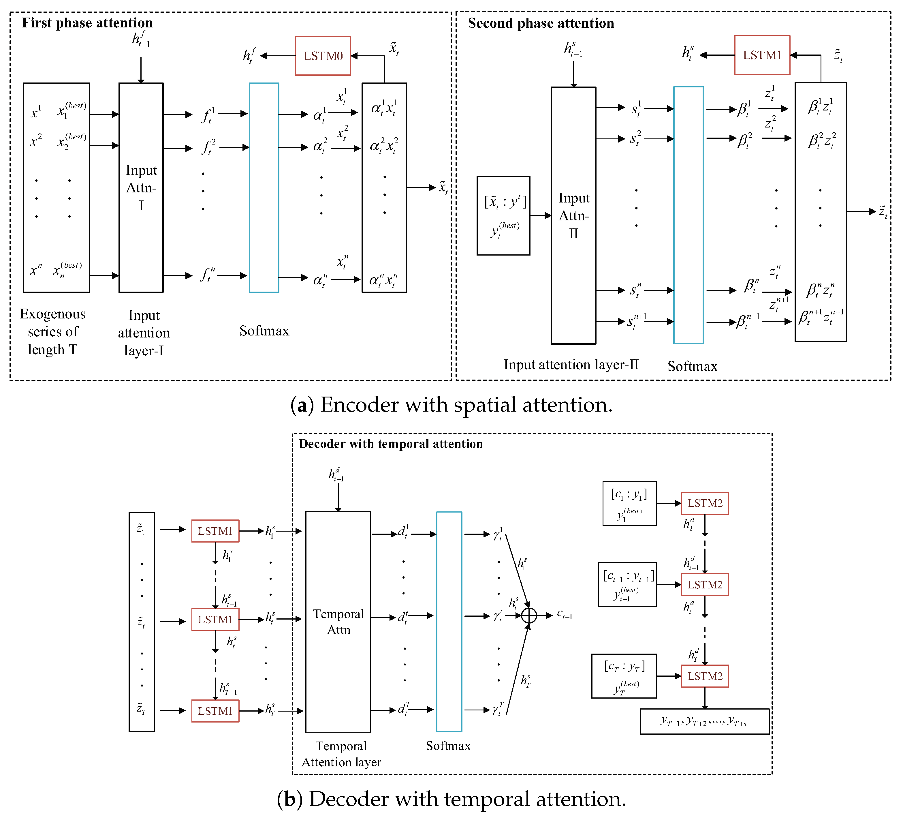
The encoder adopts the two-phase attention mechanism, aiming to learn the spatial correlation among the central site collection exogenous series, its matching sites’ exogenous series and target series. Specifically, the spatial correlation of central site collection and matching site exogenous series can be studied in the first phase attention. In the second phase attention, the weighted features are studied again, that is, the spatial correlation among the exogenous series of the central site collection, its target series and matching sites’ target series. Therefore, the two-phase spatial mechanism ensures that the learned spatial correlation is stable.

The decoder is a temporal attention mechanism, which aims to learn the temporal correlation among the encoder hidden state, central site collection target series and matching sites’ target series.

Because target and non-target have a certain influence on response selection [26], a two-phase attention mechanism is used to learn the correlation between the target series and the exogenous series in the paper. The flow chart of the improved dual-stage two-phase model based on the attention mechanism is shown in Figure 3.

(1) First phase attention

In the first phase, DSTP-RNN used the attention module to learn the spatial correlations between these exogenous attributes but all of these exogenous attributes come from the same site, the influence of exogenous series of other sites on the exogenous series of the central site is ignored. Because of the influence of wind, air pollutants from other sites will diffuse to the central site collection, resulting in the change of the exogenous series. To deal with this problem, in this paper, the data of the central site’s collection and its matching site is input into the model together, and the exogenous series relationship between them can be studied through the model, which can improve the accuracy of predicting PM${}_{2.5}$ concentration for the central site.

The matching site is determined by exogenous series correlation method, and the formulas are as follows:

$$cor{r}^k=r(x^k,y)$$

(11)

$${\lambda }^k=\frac{exp\left(cor{r}^k\right)}{{\displaystyle \sum _{j=1}^n}exp\left(cor{r}^k\right)}$$

(12)

$$f\left(i\right)=\sum _{k=1}^n{\lambda }^{k}r(x^k,x_k^{\left(i\right)})$$

(13)

$$f\left(best\right)=max\left(f\right(j\left)\right),1⩽j⩽N,$$

(14)

where $r(·)$ is the Pearson correlation coefficient, $cor{r}^k$ is the Pearson correlation coefficient of the k-th exogenous series of the site and the target series. $f\left(i\right)$ is the correlation between the exogenous series of the current site and the corresponding exogenous series of the i-th site and $f\left(best\right)$ is the best selected matching site.

Given the k-th feature $x^k$ of the central site collection at time t, the k-th feature $x_k^{\left(best\right)}$ of the best matching site exogenous series. The input attention mechanism-I is used to learn the exogenous attributes’ spatial correlation of the central site collection and the matching site:

$$f_t^k=v_f^{T}tanh(W_f[h_{t-1}^f:s_{t-1}^f]+U_f{x}^k+M_f{x}_k^{\left(best\right)}),$$

(15)

where $[*:*]$ is concatenation operation, and $v_f\in R^T,W_f\in R^{T\times 2m},U_f,M_f\in R^{T\times T}$ are the parameters to learn. $h_{t-1}^f\in R^m$ and $s_{t-1}^f\in R^m$ are the hidden state and the cell state of the encoder LSTM0 (LSTM layer in the first attention module) unit at the previous moment, respectively. m is the hidden size in the first attention module.

After $f_t^k$ is calculated, the Softmax function is used for normalization:

$${\alpha }_t^k=\frac{exp\left(f_t^k\right)}{\sum _{j=1}^{n}exp\left(f_t^j\right)},$$

(16)

where attention weight ${\alpha }_t^k$ is determined by $h_{t-1}^f$, $s_{t-1}^f$, the k-th feature $x^k$ of the current input, and the k-th feature $x_k^{\left(best\right)}$ of the best matching site, which measures the importance of the k-th feature at time t.

Compared with the input exogenous series $x_t$, for the more important k-th feature, it will be larger in ${\tilde{x}}_t$. ${\tilde{x}}_t$ is the combination of all features at time t, which is defined as follows:

$${\tilde{x}}_t={({\alpha }_t^1{x}_t^1,{\alpha }_t^2{x}_t^2,\dots ,{\alpha }_t^n{x}_t^n)}^T.$$

(17)

Then, the hidden state $h_{t-1}^f$ and ${\tilde{x}}_t$ are input into the LSTM0 layer, and the hidden state $h_t^f$ at the current moment is updated. ${\tilde{x}}_t$ is then input into the second phase attention.

(2) Second phase attention

In the second phase, more stable and concentrated correlations can be obtained through the second learning of spatial correlation. The purpose of this module is to learn the spatial correlation among the exogenous series of the central site collection, its target series and matching site target series.

In this study, the specific approach is to combine the target series of the central site collection with the exogenous series of the corresponding time, and the target series of the best matching site is added. The attention weights of the input attention mechanism-II are as follows:

$$s_t^k=v_s^{T}tanh(W_s[h_{t-1}^s:s_{t-1}^s]+U_s[{\tilde{x}}^k:y^k]+M_s{y}_k^{\left(best\right)})$$

(18)

$${\beta }_t^k=\frac{exp\left(s_t^k\right)}{{\displaystyle \sum _{j=1}^{n+1}}exp\left(s_t^j\right)},$$

(19)

where $v_s^T\in R^T,W_s\in R^{T\times 2q},U_s\in R^{T\times T},M_s\in R^T$ are parameters to learn; $h_{t-1}^s\in R^q$ and $s_{t-1}^s\in R^q$ are the hidden state and cell state of the encoder LSTM1 (LSTM layer in the second attention module) unit at the previous time; and q is the hidden size in the second attention module.

The corresponding target variable $y^k$ is concatenated to the k-th attribute ${\tilde{x}}^k$ to form a new vector $z^k$, that is $z^k=[{\tilde{x}}^k:y^k]\in R^{(n+1)\times T}$. For each spatial attention module with a target series, the above actions are taken independently.

Attention weight ${\beta }_t^k$ measures the importance of $z^k$ at time t, and any attribute value at any time has its corresponding weight:

$${\tilde{z}}_t={({\beta }_t^1{z}_t^1,{\beta }_t^2{z}_t^2,\cdots ,{\beta }_t^{n+1}{z}_t^{n+1})}^T.$$

(20)

Then, $h_{t-1}^s$ and ${\tilde{z}}_t$ are input into the LSTM1 layer. The purpose is to update the hidden state $h_t^s$ at the current moment and $h_t^s$ is input into the next stage of temporal attention.

(3) Decoder with temporal attention

The disadvantage of the traditional attention mechanism is that the context vector only relies on the hidden state at the last moment, and cannot pay attention to the important features. However, the decoder with temporal attention can adaptively select the encoder hidden state most relevant to the target series by weighting the encoder hidden state. The encoder with spatial attention outputs the hidden state, and the decoder learns the temporal relationship of the hidden state through the attention mechanism within the window size T.

Based on the hidden state $h_{t-1}^d\in R^p$ and cell state $s_{t-1}^d\in R^p$ of the decoder LSTM2 (LSTM layer in the third attention module) unit at the previous time, the attention weight of each encoder hidden state in the second attention module at time t can be calculated. The attention weights of the temporal attention mechanism are as follows:

$$d_t^i=v_d^{T}tanh(W_d[h_{t-1}^d:s_{t-1}^d]+U_d{h}_i^s+b_d)$$

(21)

$${\gamma }_t^i=\frac{exp\left(d_t^i\right)}{{\displaystyle \sum _{j=1}^T}exp\left(d_t^j\right)},$$

(22)

where $v_d,b_d\in R^p,W_d\in R^{q\times 2p},U_d\in R^{p\times p}$ are parameters to learn, p is the hidden size in the third attention module and $h_i^s\in H^s$ is the i-th encoder hidden state of the second attention module. The context vector $c_t$ is defined as follows:

$$c_t=\sum _{j=1}^T{\gamma }_t^j{h}_j^s.$$

(23)

The context vector represents the weighted sum of all hidden states in the second attention module within the window size T. DSTP-RNN combined the context vector $c_t$ with the target series Y, but the influence of the matching site target series on the decoder hidden state is ignored. In this paper, by concatenating the target series of matching site, the temporal relationship between all hidden states of the central site collection and the target series of the matching site is once again learned:

$${\tilde{y}}_{t-1}={\tilde{W}}^T[y_{t-1}:c_{t-1}]+\tilde{b}+{\tilde{H}}^T{y}_{t-1}^{\left(best\right)},$$

(24)

where ${\tilde{W}}^T\in R^{q+1}$ and $\tilde{b},{\tilde{H}}^T\in R$ are parameters that map concatenation to the size of the decoder hidden state. ${\tilde{y}}_{t-1}$ and $h_{t-1}^d$ are then input into the LSTM2 layer to update the hidden state $h_t^d$ at the current moment. The final multi-step prediction formula is as follows:

$$y_{T+1},\dots ,y_{T+\tau }=v_y^T(W_y[h_T^d:c_T]+b_y)+b_y^{\prime },$$

(25)

where $W_y\in R^{p\times (p+q)}$ and $b_y\in R^p$ are parameters that map concatenation to the size of the decoder hidden state. $[h_T^d:c_T]\in R^{p+q}$ represents the concatenation of the decoder hidden state and context vector at time T. $v_y\in R^{\tau \times p}$ is the weight, $b_y^{\prime }\in R^{\tau }$ is deviation. The linear function produces the final prediction result.

2.3. Attention-Based Layer

After getting the prediction result of each site, LSTM-FC [20] input all the results into the fully connected layer to obtain the prediction result of the central site, ignoring the correlations of PM${}_{2.5}$ concentration between neighboring sites and the central site.

In this paper, the correlation coefficients between the central site and the selected neighboring sites are introduced as attention weights in the fully connected layer, and the spatial correlations of different sites are dynamically studied. The correlation coefficient set of neighboring sites and central site is

$$M={(m_1,m_2,\cdots ,m_{a+1})}^{a+1}\in R^{a+1},$$

(26)

where a is the number of selected neighboring sites, and M is normalized by the Softmax function:

$${\omega }^k=\frac{exp\left(m_k\right)}{{\displaystyle \sum _{j=1}^{a+1}}exp\left(m_j\right)}.$$

(27)

The data of each site are input into the improved dual-stage two-phase model based on the attention mechanism, and the output matrix of the model is $H={(h_1,h_2,\cdots ,h_{a+1})}^{a+1}\in R^{a+1}$. The attention weight of learning is as follows:

$$u_k=v_{u}tanh(K_u{h}_k+b_u)$$

(28)

$${\eta }_k=\frac{exp\left(u_k\right)}{{\displaystyle \sum _{j=1}^T}exp\left(u_j\right)},$$

(29)

where $v_u,b_u,K_u$ are the parameters to learn, and s is the predicted PM${}_{2.5}$ concentration of the central site. The calculation formula is as follows:

$$s=\sum _{j=1}^{a+1}{\omega }^j{\eta }_j{h}_j.$$

(30)

3. Experimental Results

3.1. Settings

The dataset used in this paper is from the weather and air pollution index collected by the US embassy in Beijing, China from 2013 to 2017 (see http://archive.ics.uci.edu/ml/datasets/Beijing+Multi-Site+Air-Quality+Data, accessed on 20 September 2019) [27]. In the experiment of this paper, only one year of data is selected randomly from the dataset, which is from 1 April 2014 to 1 February 2015 (a total of 8760 data). It is big enough for the PM${}_{2.5}$ concentration prediction. Each air quality record contains six pollutants: PM${}_{2.5}$, PM${}_{10}$, SO${}_2$, NO${}_2$, CO and O${}_3$. Each meteorological record contains seven items—time (the interval is one hour), temperature, pressure, dew point temperature, precipitation, wind direction and wind speed. The average, median and standard deviation of PM${}_{2.5}$ concentration at the central site are 90.07 μg/m${}^3$, 68.72 μg/m${}^3$ and 83.30 μg/m${}^3$, respectively. The standard deviation is relatively large, indicating that the data are widely distributed.

The first 75% of the dataset is selected as the training data and the remaining 25% as the test data. If the continuous missing values are greater than one row, IDW interpolation [25] is used to fill the missing values according to the neighboring sites PM${}_{2.5}$ concentration. It is because PM${}_{2.5}$ concentration data from various sites are highly correlated. If the continuous missing values are less than two rows, the linear interpolation method is used.

To prove that the proposed method is more suitable for long-term prediction, the 1−24 h are divided into three time lags (1−6, 7−12 and 13−24 h) and a separate model is trained to predict the average PM${}_{2.5}$ concentration of each time lag. Each model is set with appropriate hyper parameters to produce the best performance. The predicted time lag of 1–6 h is 8, 7–12 h is 16, and 13–24 h is 28.

The back propagation algorithm is used to train all models. DIstortion Loss including shApe and TimE (DILATE) loss function [28] is used in the experiment. In the training process, the small-batch stochastic gradient descent (SGD) is combined with Adam optimizer, the size of the random small batch is set to 128, the upper limit of the training period is 200, the learning rate is set to 0.001 and the number of neighboring sites is set to 4. A layer of an LSTM network is used for each attention module, and the hidden state of the LSTM network is set to the same, that is, $m=p=q=$ 128.

In order to evaluate the effectiveness of the method, two indicators are used in the experiment, including root mean square error (RMSE) and mean absolute error (MAE). These indicators are defined as follows:

$$RMSE=\sqrt{\frac{1}{n}\sum _{i=1}^n{(y_i-{y_i}^{\prime })}^2}$$

(31)

$$MAE=\frac{1}{n}\sum _{i=1}^n\left|y_i-y_i^{\prime }\right|,$$

(32)

where $y_i$ is the true value and ${y_i}^{\prime }$ is the predicted value.

3.2. Models Comparison

The comparison results between the proposed model and other models are shown in

Table 1. Comparison of the performance of different models.

Time Methods	1–6 h		7–12 h		13–24 h
	RMSE	MAE	RMSE	MAE	RMSE	MAE
LSTM	37.38	23.45	57.93	42.63	66.39	48.15
CNN-LSTM	39.37	23.87	51.37	41.93	64.03	44.82
LSTM-FC	36.97	22.97	56.70	40.23	63.79	42.57
DA-RNN	36.29	21.40	48.07	35.57	60.81	43.53
DSTP-FC (ours)	32.51	19.50	45.22	32.22	51.45	37.04

. In this paper, some state-of-the-art models are used to test the superiority of the proposed model (DSTP-FC), which are introduced as follows. LSTM [29]: The problem of RNN gradient disappearance can be avoided and the long-term dependence in series learning can be captured. CNN-LSTM [21] used CNN to extract the actual characteristics and spatial correlation from the input data, and used LSTM to predict the future PM${}_{2.5}$ concentration. LSTM-FC [20] used the spatial combination based on fully connected neural network to integrate the prediction results of neighboring sites, and the final PM${}_{2.5}$ prediction result of the central site is given. DA-RNN [22]: Attention mechanism is introduced not only in the input stage of decoder but also in the encoder stage. The encoder stage attention mechanism realizes the function of feature selection and timing dependence.

The results in Table 1 show that the comprehensive result of LSTM-FC is better than that of LSTM, which shows that the method of using a fully connected neural network to integrate the prediction results of neighboring sites is effective. The comprehensive results of DA-RNN model are better than LSTM, LSTM-FC and CNN-LSTM models. It shows that the introduction of an attention mechanism in encoder and decoder can better grasp the timing dependence. At the same time, the comprehensive results of the proposed DSTP-FC model in this paper are better than that of DA-RNN, which shows the effectiveness of the proposed model.

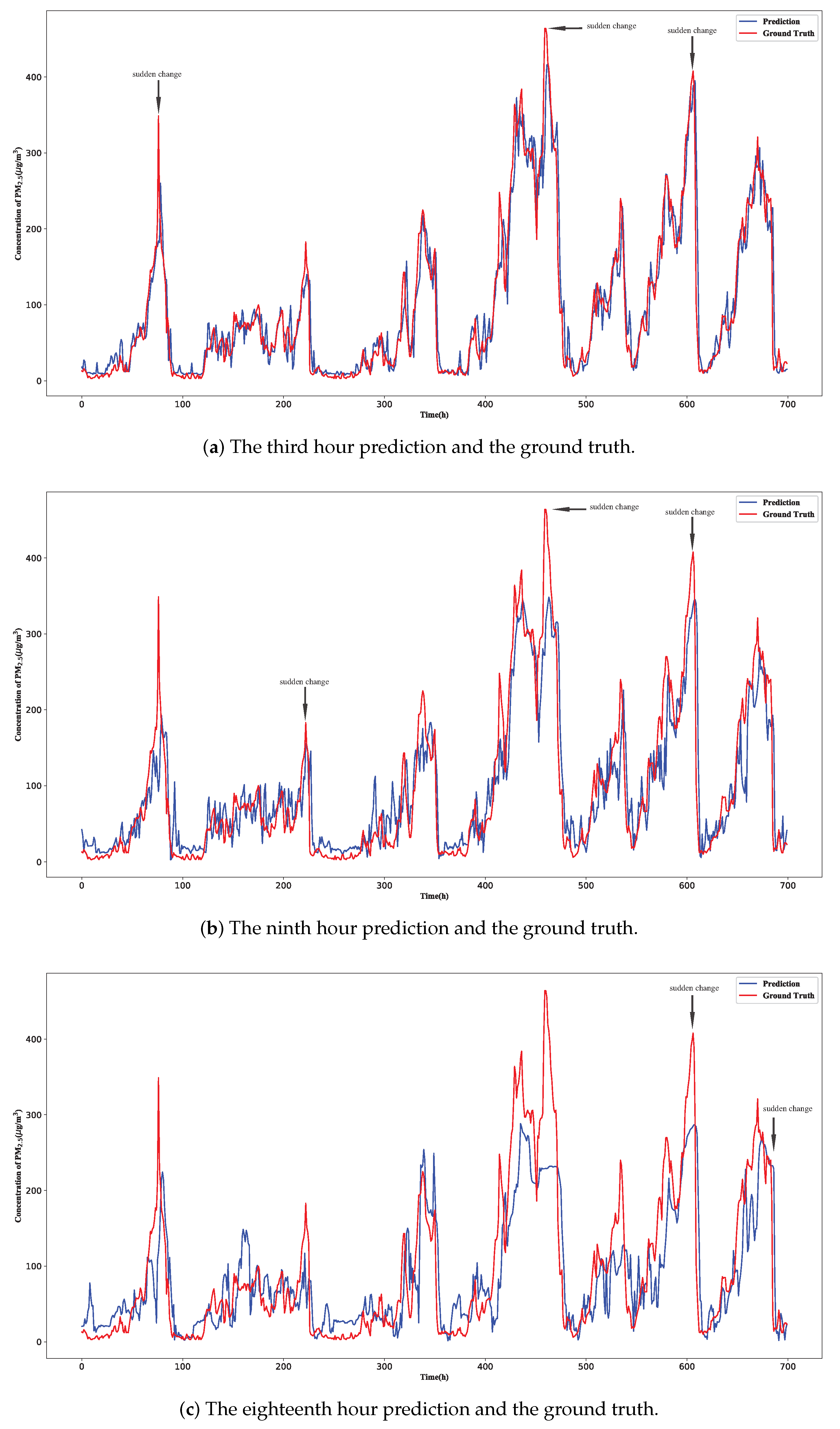
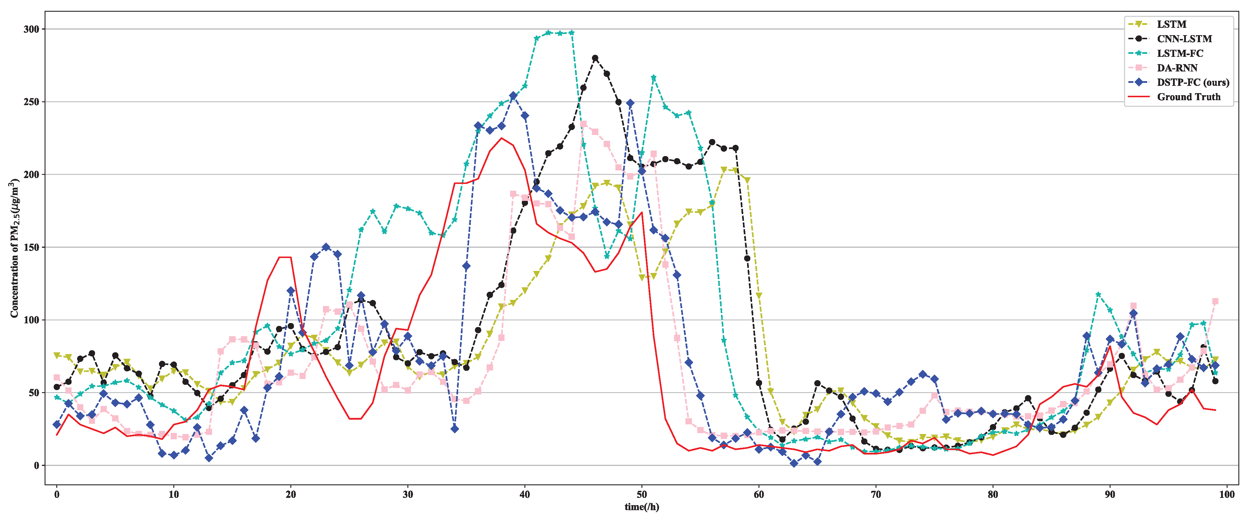
To show the performance of the proposed method, the prediction results of PM${}_{2.5}$ concentration at the central site from 1 November 2014 to 30 November 2014 based on the proposed model are shown in Figure 4, where the deviations between the prediction of the model and ground truth increase with the increase of prediction time. The reason to select this time frame to visualize model prediction is that the change of the PM${}_{2.5}$ concentration in the winter of China is very big. There are several sudden change points of PM${}_{2.5}$ concentration in the figure, and it can be seen that PM${}_{2.5}$ concentration changes obviously. For example, the PM${}_{2.5}$ concentration decreases by nearly 187 g/m${}^3$ in one hour, but the proposed DSTP-FC model can give out accurate prediction results. To further show the performances of the PM${}_{2.5}$ concentration prediction using different methods, one scatter plot is shown in Figure 5. Here, only the eighteenth hour prediction of the PM${}_{2.5}$ concentration for a total of 100 h is given out, to make the paper more readable. It is easy to see that the performance of the proposed model is better than other methods.

3.3. Ablation Experiment

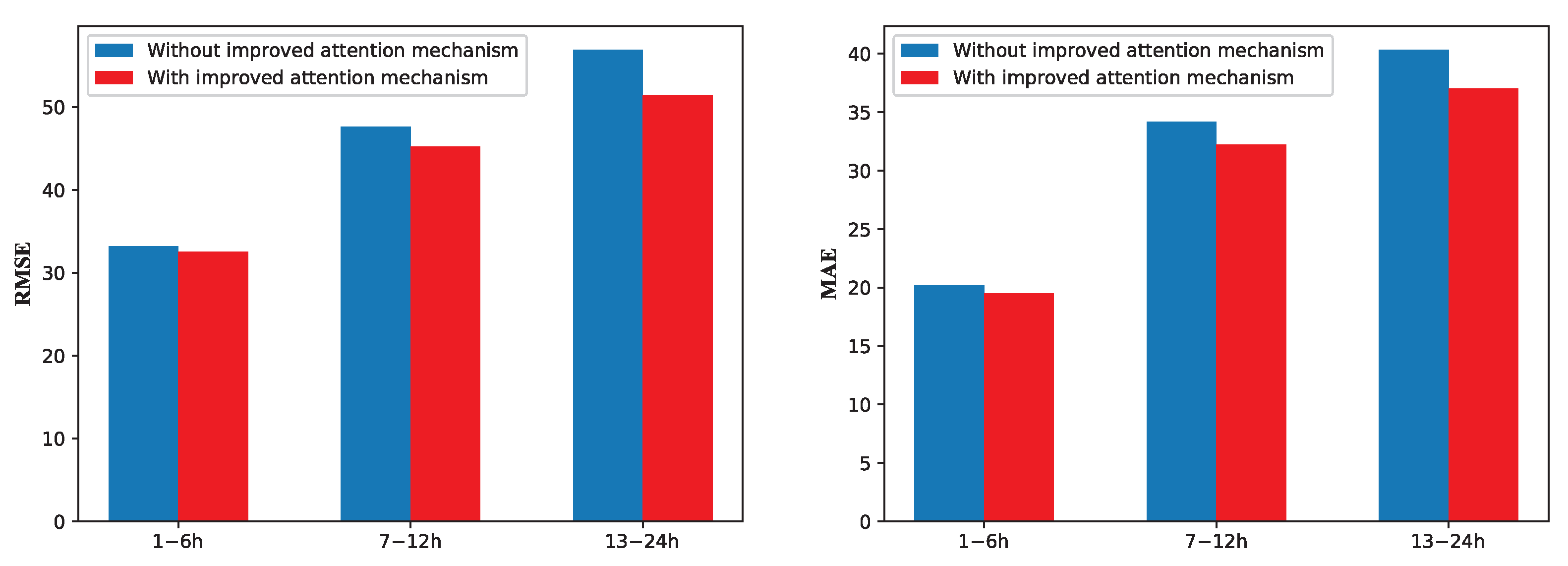
The effect of the proposed model with the improved attention mechanism on the experimental accuracy is shown in Figure 6. It can be seen from the figure that the improved attention mechanism greatly improves the accuracy of the model in the medium and long-term PM${}_{2.5}$ concentration prediction, the reasons are as follows.

Firstly, according to the exogenous series correlation method, the data of the most relevant sites are dynamically combined, and the influence of the relevant sites exogenous series on the central site collection is considered. Secondly, the attention mechanism is added to the fully connected layer, the accuracy of PM${}_{2.5}$ prediction at the central site can be improved by combining the correlation coefficients between neighboring sites and the central site. However, in the short-term prediction of 16 h, the experimental accuracy is improved to a limited extent by the improved attention mechanism. This is because the time step is relatively small and the dynamic combination of data from the most relevant sites increases the redundant data. The comprehensive results verify the validity of the proposed model.

4. Discussions

The experiments in Section 3 show that the proposed model has better performance than the state-of-the-art models in the PM${}_{2.5}$ concentration prediction. In this section, the performances of the proposed approach are discussed on the key parts of the proposed model, including the spatio-temporal correlation, the time steps and the loss functions.

4.1. About the Spatio-Temporal Correlation

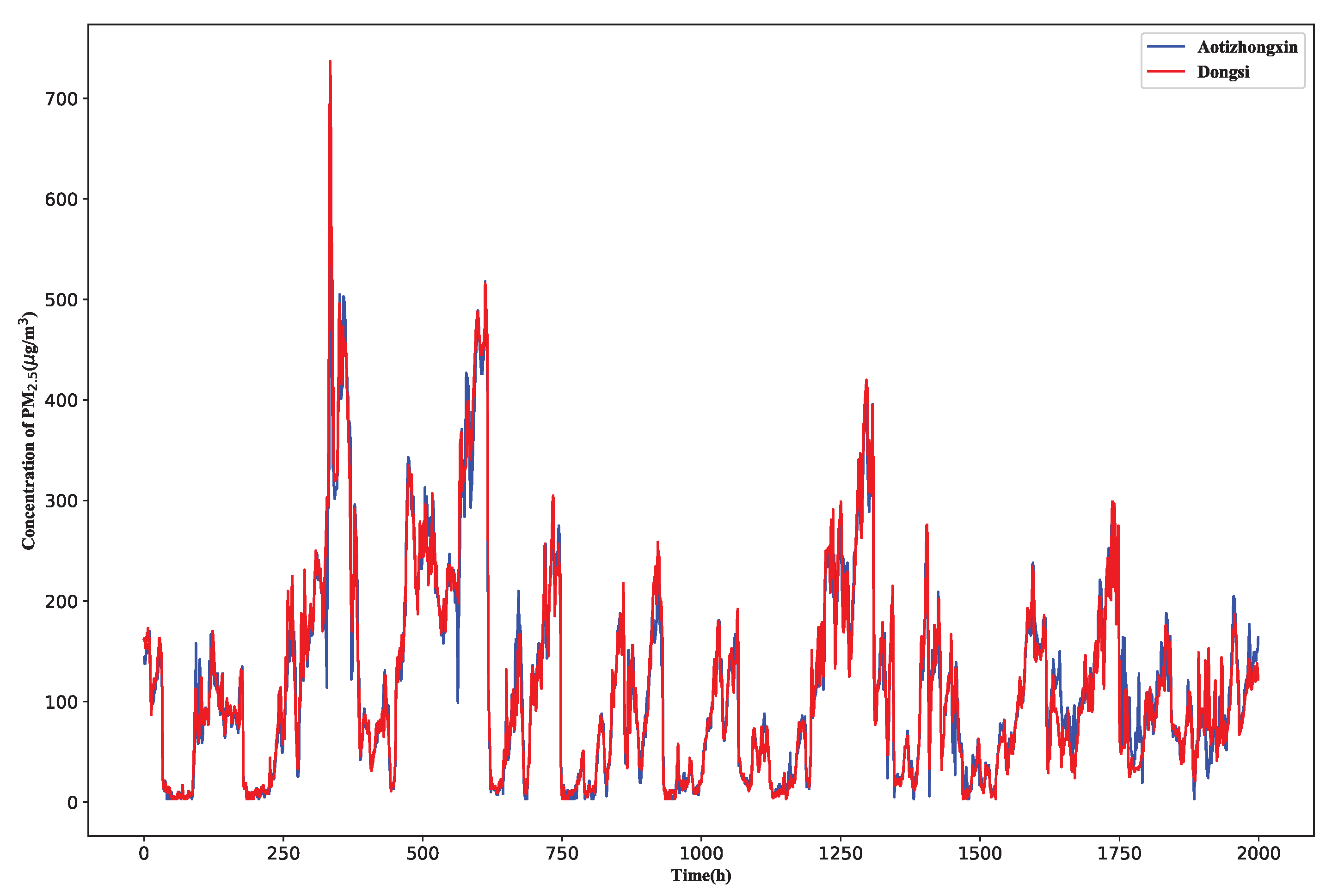
In the spatio correlation analysis, Granger causality test [30] is often used to analyze the causality between series of different sits. To discuss the effectiveness of the Granger causality test based method in the PM${}_{2.5}$ concentration prediction, the PM${}_{2.5}$ concentration of each site is analyzed in this paper. The results show that the pollution trends are highly similar, without time delay. One example of the comparison of PM${}_{2.5}$ concentration between Aotizhongxin and Dongsi sites is shown in Figure 7. The MAE and RMSE of these two sites PM${}_{2.5}$ concentration are 14 and 23.2, respectively, so the PM${}_{2.5}$ concentration of each site reflects the similarity rather than the causality. The result means that the Granger causality test is not effective in the spatio correlation analysis. In this paper, Pearson correlation coefficient is used to measure the spatial correlation of PM${}_{2.5}$ concentration at 12 sites. The results show that all correlation values are higher than 0.80 (p-value < 0.05), indicating that there is a high correlation between PM${}_{2.5}$ concentrations among sites, which means the PM${}_{2.5}$ concentration of neighboring sites is helpful to predict the PM${}_{2.5}$ concentration at the central site.

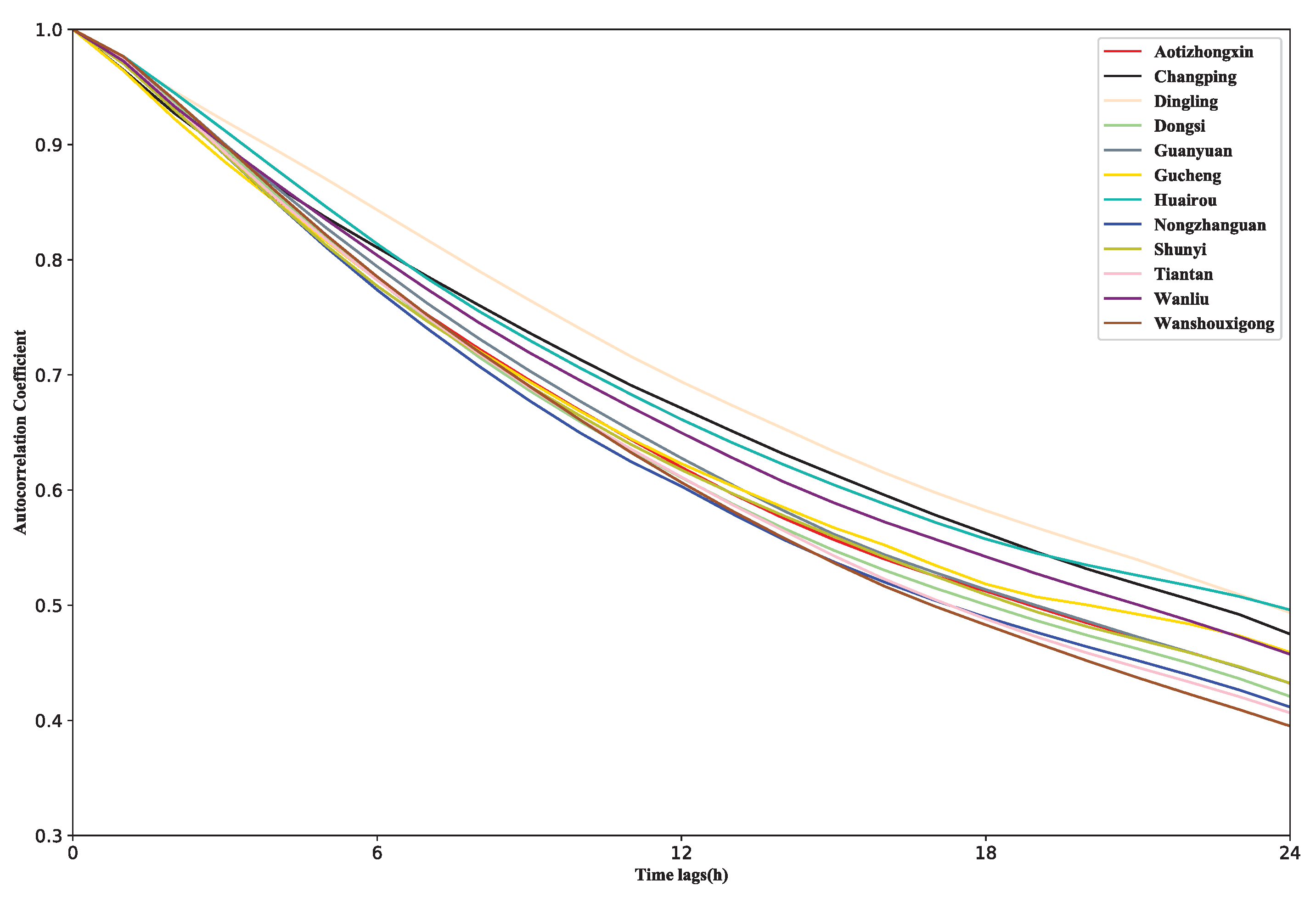
In the time correlation analysis, the autocorrelation function is used in this paper to measure the time correlation between PM${}_{2.5}$ concentration time series at each site. It can be seen from Figure 8 that the autocorrelation coefficient of PM${}_{2.5}$ concentration after 24 h is above 0.4, and the correlation is moderate or above. Therefore, it is feasible to predict PM${}_{2.5}$ concentration within 24 h with historical data. In addition, the autocorrelation coefficient of each site in the figure decreases with the increase of time lags. Earlier events have less impact on the current state.

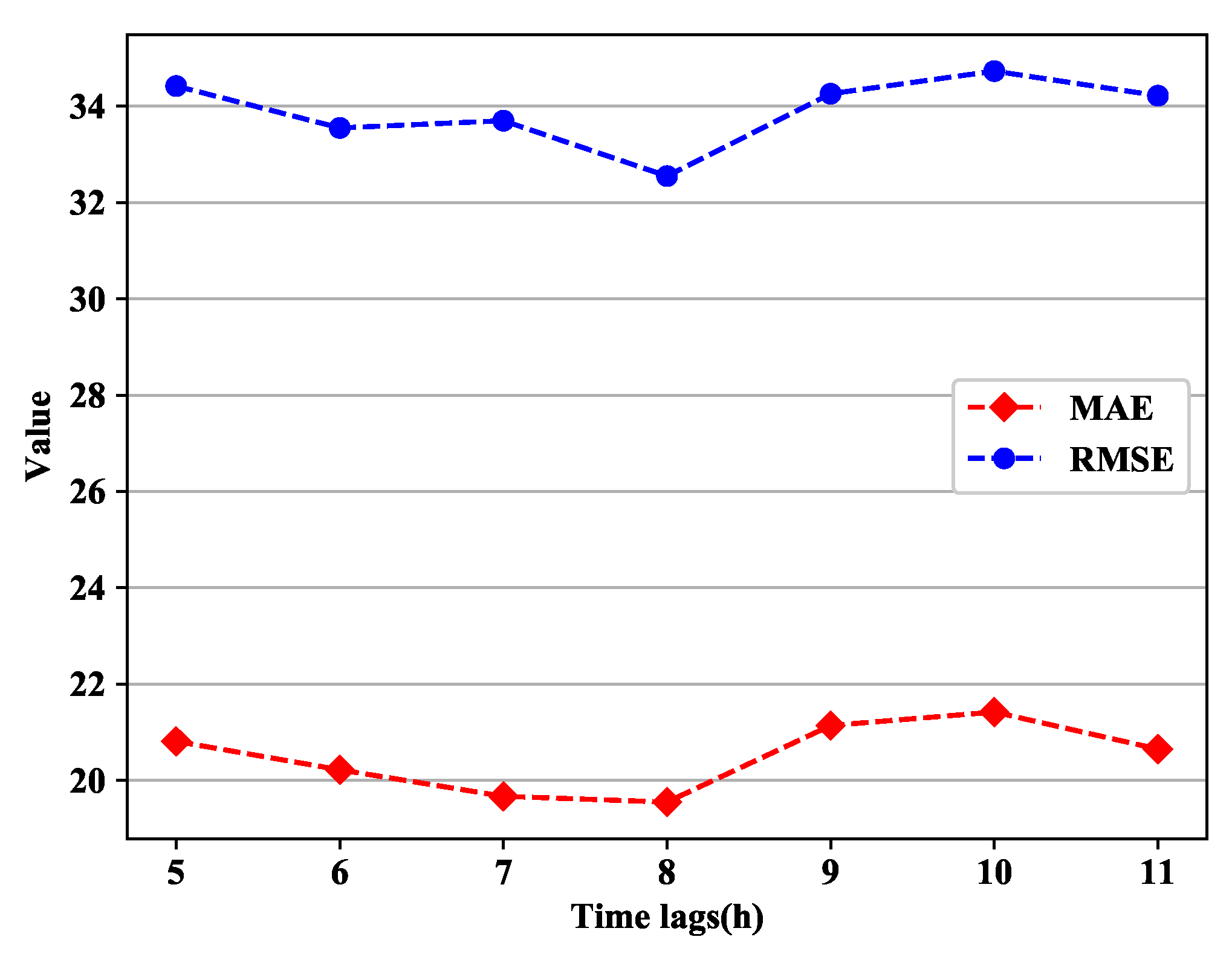
4.2. About the Time Steps

Different time steps are selected for different time lags. This is because with the increase of time step, more unrelated variables will be input and the prediction accuracy will be reduced. If the time lag is too small, the input information will be insufficient. Here, an example of choosing the best time step in different time lags is illustrated. As shown in Figure 9, the RMSE and MAE values vary with the size of the time step. Obviously, the lowest RMSE and MAE values are obtained in the scatter plot when the predicted time step is 8 within 1–6 h, and a similar method can be used to determine the time steps of other times.

4.3. About the Loss Functions

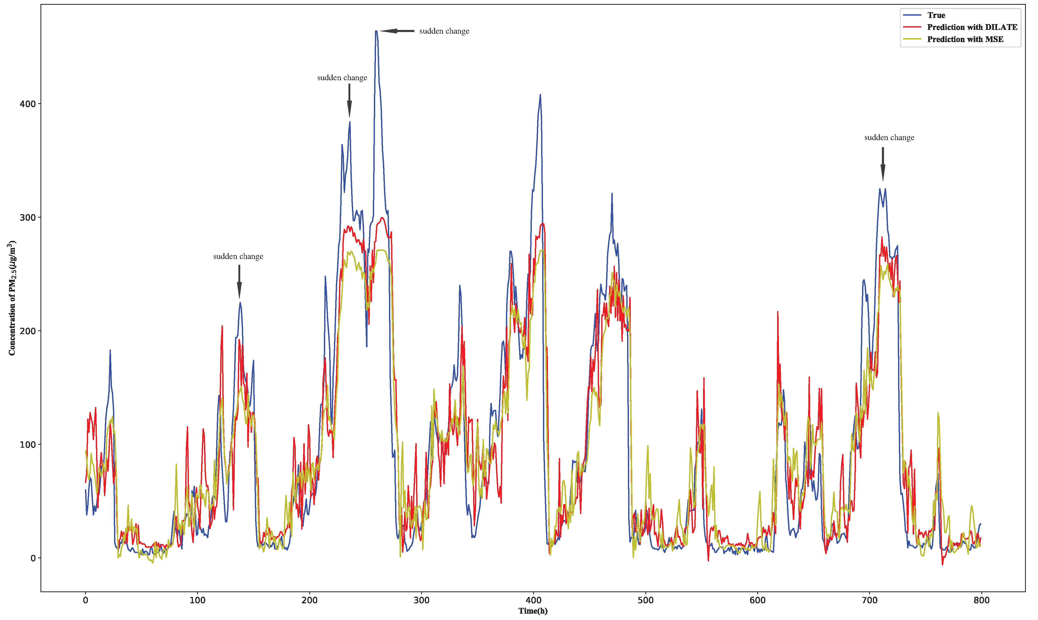
The comparative results among different loss functions are shown in

Table 2. Comparison of prediction accuracy of PM${}_{2.5}$ concentration using different loss functions.

Time Methods	1–6 h		7–12 h		13–24 h
	RMSE	MAE	RMSE	MAE	RMSE	MAE
DSTP-FC-MAE	35.36	21.03	48.13	34.66	54.03	43.25
DSTP-FC-MSE	34.55	20.42	44.17	31.93	52.79	39.46
DSTP-FC-DILATE	32.51	19.50	45.22	32.22	51.45	37.04

. The accuracy of the MAE loss function is much lower than that of DILATE and MSE loss functions. Experimental accuracy of DILATE loss function within 1–6 h and 13–24 h are better than MSE, and it is slightly worse than MSE within 7–12 h. As shown in Figure 10, the DILATE and MSE loss functions are used to predict PM${}_{2.5}$ concentration after 9 h. It can be seen that the sudden change of PM${}_{2.5}$ concentration can be better predicted with the DILATE loss function. Therefore, the comprehensive results of the DILATE loss function are the best.

4.4. About the Cross Validation

To further test the robustness of the proposed method, a 10-fold cross-validation experiment was carried out. In this cross validation experiment, the dataset was divided into 11 subset without changing the order. Then the first subset was used to predict the second subset, and the first two subsets were used as the training set to predict the third subset, and so on. The cross validation experimental results are shown in

Table 3. The experimental results of the cross validation.

Time	1–6 h		7–12 h		13–24 h
	RMSE	MAE	RMSE	MAE	RMSE	MAE
Cross validation	33.67	22.20	42.39	32.15	49.90	38.40

. The results of this experiment are close to those of Section 3.2 (see Table 1), which show that the proposed method has good robustness.

5. Conclusions and Future Work

In this paper, based on historical air quality data and meteorological data, an improved integrated deep neural network method based on an attention mechanism is proposed to predict PM${}_{2.5}$ concentration within 24 h. Due to the spread of air pollution, air quality at one site may be affected by other sites. Pearson correlation coefficient is used to learn the spatial correlation between sites and select neighboring sites. The exogenous series correlation method is used to learn the correlation between the exogenous series of other sites and the central site collection. In order to evaluate the performance of DSTP-FC model, PM${}_{2.5}$ concentration of Beijing central site is predicted. Compared with other models, the proposed model provides better prediction results based on RMSE and MAE indicators. This study can draw several useful findings: (1) compared with LSTM, LSTM-FC and CNN-LSTM, DA-RNN and DSTP-FC models with attention mechanism show better prediction performance; (2) Compared with the MSE loss function, sudden changes in PM${}_{2.5}$ concentration can be better predicted when using the DILATE loss function; (3) The target series of the central site is also affected by exogenous series of other sites.

In our future work: (1) More factors should be considered, such as the sudden emission of air pollutants in the factory, so the law of PM${}_{2.5}$ concentration change can be better studied and the sudden change of PM${}_{2.5}$ concentration can be accurately predicted; (2) The LSTM structure is used as one of the basic units in the attention module of the model, and other RNN structures can be tried; (3) In order to verify the universality of the proposed model, the monitoring sites’ data of other cities should be used for experiments.

References

- Chen, Z.; Cui, L.; Cui, X.; Li, X.; Yu, K.; Yue, K.; Dai, Z.; Zhou, J.; Jia, G.; Zhang, J. The association between high ambient air pollution exposure and respiratory health of young children: A cross sectional study in Jinan, China. Sci. Total Environ. 2019, 656, 740–749. [Google Scholar] [CrossRef]
- Zhang, C.; Di, L.; Sun, Z.; Lin, L.; Yu, E.; Gaigalas, J. Exploring cloud-based Web Processing Service: A case study on the implementation of CMAQ as a Service. Environ. Model. Softw. 2019, 113, 29–41. [Google Scholar] [CrossRef]
- Mathur, R.; Xing, J.; Gilliam, R.; Sarwar, G.; Hogrefe, C.; Pleim, J.; Pouliot, G.; Roselle, S.; Spero, T.L.; Wong, D.C.; et al. Extending the Community Multiscale Air Quality (CMAQ) Modeling System to Hemispheric Scales: Overview of Process Considerations and Initial Applications. Atmos. Chem. Phys. 2017, 17, 12449–12474. [Google Scholar] [CrossRef] [PubMed] [Green Version]
- Hsu, C.H.; Cheng, F.Y.; Chang, H.Y.; Lin, N.H. Implementation of a dynamical NH3 emissions parameterization in CMAQ for improving PM2.5 simulation in Taiwan. Atmos. Environ. 2019, 218, 116923. [Google Scholar] [CrossRef]
- Kurt, A.; Oktay, A.B. Forecasting air pollutant indicator levels with geographic models 3 days in advance using neural networks. Expert Syst. Appl. 2010, 37, 7986–7992. [Google Scholar] [CrossRef]
- Wang, Q.; Zeng, Q.; Tao, J.; Sun, L.; Zhang, L.; Gu, T.; Wang, Z.; Chen, L. Estimating PM2.5 Concentrations Based on MODIS AOD and NAQPMS Data over Beijing-Tianjin-Hebei. Sensors 2019, 19, 1207. [Google Scholar] [CrossRef] [Green Version]
- Wu, J.B.; Wang, Z.; Wang, Q.; Li, J.; Xu, J.; Chen, H.; Ge, B.; Zhou, G.; Chang, L. Development of an on-line source-tagged model for sulfate, nitrate and ammonium: A modeling study for highly polluted periods in Shanghai, China. Environ. Pollut. 2017, 221, 168–179. [Google Scholar] [CrossRef]
- Stadlober, E.; Hoermann, S.; Pfeiler, B. Quality and performance of a PM10 daily forecasting model. Atmos. Environ. 2008, 42, 1098–1109. [Google Scholar] [CrossRef]
- Martin, F.; Palomino, I.; Vivanco, M.G. Combination of measured and modelling data in air quality assessment in Spain. Int. J. Environ. Pollut. 2012, 49, 36–44. [Google Scholar] [CrossRef]
- Yuchi, W.; Gombojav, E.; Boldbaatar, B.; Galsuren, J.; Enkhmaa, S.; Beejin, B.; Naidan, G.; Ochir, C.; Legtseg, B.; Byambaa, T.; et al. Evaluation of random forest regression and multiple linear regression for predicting indoor fine particulate matter concentrations in a highly polluted city. Environ. Pollut. 2019, 245, 746–753. [Google Scholar] [CrossRef]
- Vanderschelden, G.; De Foy, B.; Herring, C.; Kaspari, S.; Vanreken, T.; Jobson, B. Contributions of wood smoke and vehicle emissions to ambient concentrations of volatile organic compounds and particulate matter during the Yakima wintertime nitrate study. J. Geophys. Res. Atmos. 2017, 122, 1871–1883. [Google Scholar] [CrossRef]
- Chelani, A.B. Estimating PM2.5 concentration from satellite derived aerosol optical depth and meteorological variables using a combination model. Atmos. Pollut. Res. 2019, 10, 847–857. [Google Scholar] [CrossRef]
- Wen, C.; Liu, S.; Yao, X.; Peng, L.; Li, X.; Hu, Y.; Chi, T. A novel spatiotemporal convolutional long short-term neural network for air pollution prediction. Sci. Total Environ. 2019, 654, 1091–1099. [Google Scholar] [CrossRef]
- Wang, P.; Liu, Y.; Qin, Z.; Zhang, G. A novel hybrid forecasting model for PM10 and SO2 daily concentrations. Sci. Total Environ. 2015, 505, 1202–1212. [Google Scholar] [CrossRef]
- Alimissis, A.; Philippopoulos, K.; Tzanis, C.; Deligiorgi, D. Spatial estimation of urban air pollution with the use of artificial neural network models. Atmos. Environ. 2018, 191, 205–213. [Google Scholar] [CrossRef]
- Zhu, S.; Lian, X.; Liu, H.; Hu, J.; Wang, Y.; Che, J. Daily air quality index forecasting with hybrid models: A case in China. Environ. Pollut. 2017, 231, 1232–1244. [Google Scholar] [CrossRef] [PubMed]
- Yan, R.; Liao, J.; Yang, J.; Sun, W.; Nong, M.; Li, F. Multi-hour and multi-site air quality index forecasting in Beijing using CNN, LSTM, CNN-LSTM, and spatiotemporal clustering. Expert Syst. Appl. 2021, 169, 114513. [Google Scholar] [CrossRef]
- Mao, W.; Wang, W.; Jiao, L.; Zhao, S.; Liu, A. Modeling air quality prediction using a deep learning approach: Method optimization and evaluation. Sustain. Cities Soc. 2021, 65, 102567. [Google Scholar] [CrossRef]
- Kim, M.H.; Kim, Y.S.; Lim, J.J.; Kim, J.T.; Sung, S.W.; Yoo, C.K. Data-driven prediction model of indoor air quality in an underground space. Korean J. Chem. Eng. 2010, 27, 1675–1680. [Google Scholar] [CrossRef]
- Zhao, J.; Deng, F.; Cai, Y.; Chen, J. Long short-term memory—Fully connected (LSTM-FC) neural network for PM2.5 concentration prediction. Chemosphere 2019, 220, 486–492. [Google Scholar] [CrossRef] [PubMed]
- Qin, D.; Yu, J.; Zou, G.; Yong, R.; Zhao, Q.; Zhang, B. A Novel Combined Prediction Scheme Based on CNN and LSTM for Urban PM2.5 Concentration. IEEE Access 2019, 7, 20050–20059. [Google Scholar] [CrossRef]
- Qin, Y.; Song, D.; Chen, H.; Cheng, W.; Cottrell, G.W. A Dual-Stage Attention-Based Recurrent Neural Network for Time Series Prediction. In Proceedings of the Twenty-Sixth International Joint Conference on Artificial Intelligence, Melbourne, Australia, 19–25 August 2017. [Google Scholar]
- Liu, Y.; Gong, C.; Yang, L.; Chen, Y. DSTP-RNN: A dual-stage two-phase attention-based recurrent neural network for long-term and multivariate time series prediction. Expert Syst. Appl. 2020, 143, 113082. [Google Scholar] [CrossRef]
- Guo, H.; Wang, Y.; Zhang, H. Characterization of criteria air pollutants in Beijing during 2014–2015. Environ. Res. 2017, 154, 334–344. [Google Scholar] [CrossRef] [PubMed]
- Ma, J.; Cheng, J.C.; Lin, C.; Tan, Y.; Zhang, J. Improving air quality prediction accuracy at larger temporal resolutions using deep learning and transfer learning techniques. Atmos. Environ. 2019, 214, 116885. [Google Scholar] [CrossRef]
- Hubner, R.; Steinhauser, M.; Lehle, C. A Dual-Stage Two-Phase Model of Selective Attention. Psychol. Rev. 2010, 117, 759–784. [Google Scholar] [CrossRef] [Green Version]
- Li, T.; Hua, M.; Wu, X. A Hybrid CNN-LSTM Model for Forecasting Particulate Matter (PM2.5). IEEE Access 2020, 8, 26933–26940. [Google Scholar] [CrossRef]
- Le Guen, V.; Thome, N. Shape and Time Distortion Loss for Training Deep Time Series Forecasting Models. In Proceedings of the NeurIPS, Vancouver, BC, Canada, 8–14 December 2019. [Google Scholar]
- Hochreiter, S.; Schmidhuber, J. Long Short-Term Memory. Neural Comput. 1997, 9, 1735–1780. [Google Scholar] [CrossRef]
- Wang, J.; Song, G. A Deep Spatial-Temporal Ensemble Model for Air Quality Prediction. Neurocomputing 2018, 314, 198–206. [Google Scholar] [CrossRef]
Figure 1.
Distribution of air quality sites in Beijing.
Figure 2.
The framework of the proposed DSTP-FC model.
Figure 3.
Flow chart of improved dual-stage two-phase model based on attention mechanism.
Figure 4.
The prediction results of PM concentration at the central site from 1 November 2014 to 30 November 2014 based on the proposed DSTP-FC model.
Figure 5.
The eighteenth hour prediction using different methods for a total of 100 h.
Figure 6.
Effect of the improved attention mechanism.
Figure 7.
Concentrations of PM in Aotizhongxin and Dongsi sites.
Figure 8.
Autocorrelation coefficients at the current time and 1−24 h for all sites.
Figure 9.
MAE and RMSE of DSTP-FC models with different time lags.
Figure 10.
Comparison of using DILATE and MSE loss functions to predict PM concentration after 9 h.