Vibration-Based Locomotion of an Amphibious Robot

Abstract

In this research, an innovative robot is presented that can move both on land and water thanks to a vibration-based locomotion mechanism. The robot consists of a U-shaped beam made of spring steel, two low-density feet that allow it to stand on the water surface without sinking, and a micro-DC motor with eccentric mass, which excites vibrations. The robot exhibits stable terrestrial and aquatic locomotion based on the synchronization between body vibrations and the centrifugal force due to the eccentric mass. On the one hand, in aquatic locomotion, the robot advances thanks to floating oscillations and the asymmetric shape of the floating feet. On the other hand, the terrestrial locomotion, which has already been demonstrated for a similar robot, exploits the modes of vibration of the elastic beam. In this study, the effect of different excitation frequencies on the locomotion speed in water is examined by means of experimental tests and a numerical model. A good agreement between experimental and numerical results is found. The maximum locomotion speed takes place when the floating modes of vibration are excited.

1. Introduction

Humanity has found the most effective way to move on land with the invention of the wheel. However, the need to move in different environments where wheeled vehicles cannot move forces scientists to develop mechanisms that mimic living things. Although a very small part of the Earth’s surface is suitable for the locomotion of wheeled vehicles, living things can reach almost all surfaces of the world due to their unique physiology. Today, robots can perform different locomotion movements, such as walking, running, jumping, and swimming, that mimic living things. However, today’s robots can perform these movements by consuming a large amount of energy, while living things can perform more complex and stable locomotion using much less energy. Therefore, it is important to understand the principles of animal locomotion to develop robots with low energy consumption. Research on this subject has focused on the energy consumed during locomotion [1,2,3,4,5]. The studies on the locomotion of legged robots have been mainly in the form of detailed examination of the movements of animals and the physical models related to these movements [6].

Legged robots can be divided into three main families. There are robots equipped with rigid limbs, whose locomotion is essentially based on rigid body dynamics. They have been extensively studied since the last decades of the last century [7,8,9,10]. There are hopping robots that mimic hopping locomotion used by many animals, especially at high speeds. Hopping locomotion requires the presence of elastic limbs able to store elastic energy [10,11,12]. Finally, there are soft robots, which are the most recent family. They have some characteristics of the hopping robots, but they also mimic the behavior of many animals that adjust the stiffness and shape of their limbs in order to increase their mobility [13,14,15,16].

The first issue of this research is vibration-based locomotion. Since this kind of locomotion shares many features and problems with hopping locomotion, a brief literature review on this topic is presented. The first research on hopping robots was carried out in the 1980s at the Leg Lab of the MIT [10]. As a result of these studies, robot mechanisms capable of two-dimensional and three-dimensional locomotion have been developed, but these mechanisms had complex structures and showed excessive energy consumption. In contrast, appropriately designed elastic limb mechanisms allow the development of legged robots with lower energy consumption by exploiting a natural vibration, and the energy efficiency of these systems may approach one of biological organisms [17]. The use of elastic limbs in robots brings energy efficiency together with a range of control difficulties. This difficulty can be eliminated by overlapping frequencies of the free vibrations of the elastic limbs and the periodic actuation of the robot. The identification of the stiffness properties of hopping robots is very important in order to generate accurate dynamic models, and, for this purpose, Experimental Modal Analysis (EMA) can be used [18,19]. In recent years, many robotic systems with elastic limbs have been developed [20,21,22,23,24,25]. For example, Bhatti et al. have developed a simple but effective control unit for a single-legged hydraulic robot, which can change the jump height, step length, and, thus, the flight time [21]. Li et al. presented a soft-bodied jumping robot called JelloCube, which can be used for applications that require locomotion on uneven terrain [22]. Using a free vibration mode, Reis et al. have developed an elastic mechanism that can perform locomotion with low energy consumption [23,24,25].

The second main issue of this research is amphibious locomotion [26,27,28,29,30]. The locomotion mechanism of many amphibious robots has been developed by taking inspiration from living things. The nervous system of amphibious animals has been studied, and a robot motion control system that can control movement patterns such as walking, breathing, and swimming has been developed and applied to a multi-foot amphibious robot [31]. In Reference [32], an amphibious spherical robot inspired by amphibious turtles was developed. The six-pedal amphibious robot [33], which is a four-legged salamandra robot [34] inspired by a cockroach, and the six-legged amphibious robot (AmphiHex-I) [35] are some of the most well-known examples of a robot mimicking nature. Zhong et al. introduced an amphibious robot mechanism (AmphiHex-II) with semi-circular stiffness adjustable feet [36]. In Reference [37], an alligator-inspired robot was developed. Liquids have surface tension due to the strong cohesive force between their molecules. The surface tension of water is about ten times greater than the weight of some aquatic organisms with a body mass of milligrams. This makes it possible for aquatic insects to move on the water surface, and even to jump on it. Using this characteristic of the water, Koh et al. [38] developed a water strider robot. In the robot design, a simple mechanical model of the interaction between the water strider’s legs and the water surface is established. Moreover, Yang et al. [39] developed a theoretical leg motion model that provides an estimate of conditions for optimal jump performance of water runners.

This research deals with a simple two-legged robot, which consists of a U-shaped elastic beam, two feet, and a micro-DC motor with eccentric mass. Due to the shape and material of the feet, the robot can move both on land and in the water. Potential applications include the use of this robot to transport environmental sensors from ground to water (e.g., sensors for bridge monitoring in lagoons), and the collection and transport of plastic waste from shallow water to ground. This paper chiefly focuses on the aquatic locomotion of the amphibious robot. First, in order to have a better understanding of the locomotion principle, the natural frequencies and the modes of vibration of the amphibious robot are analytically derived. Since the terrestrial locomotion capabilities of this kind of robot have been already demonstrated in References [23,24,25], the aim of the analysis is to demonstrate that, in the aquatic locomotion, the structural stiffness of the robot can be neglected. Then, a multi-body model of the robot is developed, in order to study the aquatic locomotion principle in detail. Many numerical results dealing with forces and displacements of the robot feet and locomotion speed are presented. Finally, experimental tests are described. The experimental results show that the robot has both terrestrial and aquatic locomotion capabilities, owing to the developed foot structure. The measured locomotion speed as a function of the frequency of the rotating mass and the natural frequencies of the robot are in good agreement with the results coming from the mathematical and numerical models.

2. Amphibious Robot

The amphibious robot considered in the framework of this research is an improvement of the U-shaped walking robot presented in References [23,25]. The experimental results presented in these references showed that the robot was able to walk on the ground exploiting the elastic deformability of the U-shaped beam.

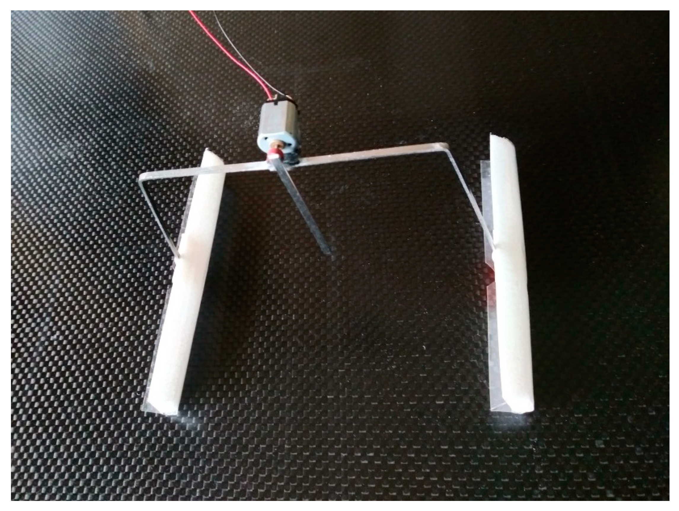
The photograph of the amphibious robot is shown in Figure 1 and its main dimensions and inertial properties are summarized in

Table 1. Main design parameters of the amphibious robot.

$m_{motor}$	3 g	$I_{top}$	1114 g·mm2
$m_{spine}$	1 g	$r_p$	25 mm
$m_{leg}$	1 g	$L_v$	75 mm
$m_p$	0.7 g	$L_h$	85 mm
$m_f$	0.4 g	$L_p$	90 mm
$m_h$	0.4 g	a	0.8 mm
$m_{tot}$	7.5 g	b	2 mm
$r_1$	10 mm	E	200 GPa
$r_2$	7 mm

. The dimensions of the robot are different from the ones presented in References [23,25] and, moreover, half-elliptical feet are introduced in order to obtain aquatic locomotion. The robot consists of a U-shaped beam, a micro-DC motor with mass $m_{motor}$, and two feet with mass $m_f$ = $m_h$ made of polyurethane foam. The legs (length $L_v$ and mass $m_{leg}$) and spine (length $L_h$ and mass $m_{spine}$) of the robot are made of spring steel (Young modulus $E$ = 200 GPa) with a cross section of $a$ = 0.8 mm × $b$ = 2 mm and formed as a U-shaped beam with right angles. The micro-DC motor is mounted at the center of the spine and a small eccentric mass ($m_p$ at a radius $r_p$) is driven by the motor. The robot is supported by two floating feet made of low-density material that enable the robot to move both on land and on the water surface. The polyurethane feet with a half-elliptical section (with semiaxes $r_1$ and $r_2$ and length $L_p$) are submerged in water by 50% while statically carrying the robot total mass $m_{tot}$ = 7.5 g.

The following assumptions were made [25] in order to develop a mathematical model of the robot for terrestrial locomotion: the behavior of the robot can be analyzed in the sagittal plane, the contact of the feet with the ground can be considered as a point contact, the elastic properties of the spline and legs are represented by lumped linear and torsion springs, and the mass properties of the system are represented by lumped masses.

The physical principle of aquatic locomotion is rather different from the physical principle of terrestrial locomotion [25] and, in particular, buoyancy and drag forces play a very important role. New modes of vibration related to floating do appear and influence locomotion. Therefore, the modes of vibration due to elastic deformability are first analyzed with a detailed model, in order to evaluate their possible influence on aquatic locomotion. Then, the typical modes of vibration related to floating are analyzed.

3. Natural Frequencies and Modes of Vibration

3.1. Modes of Vibration Due to Elastic Deformability

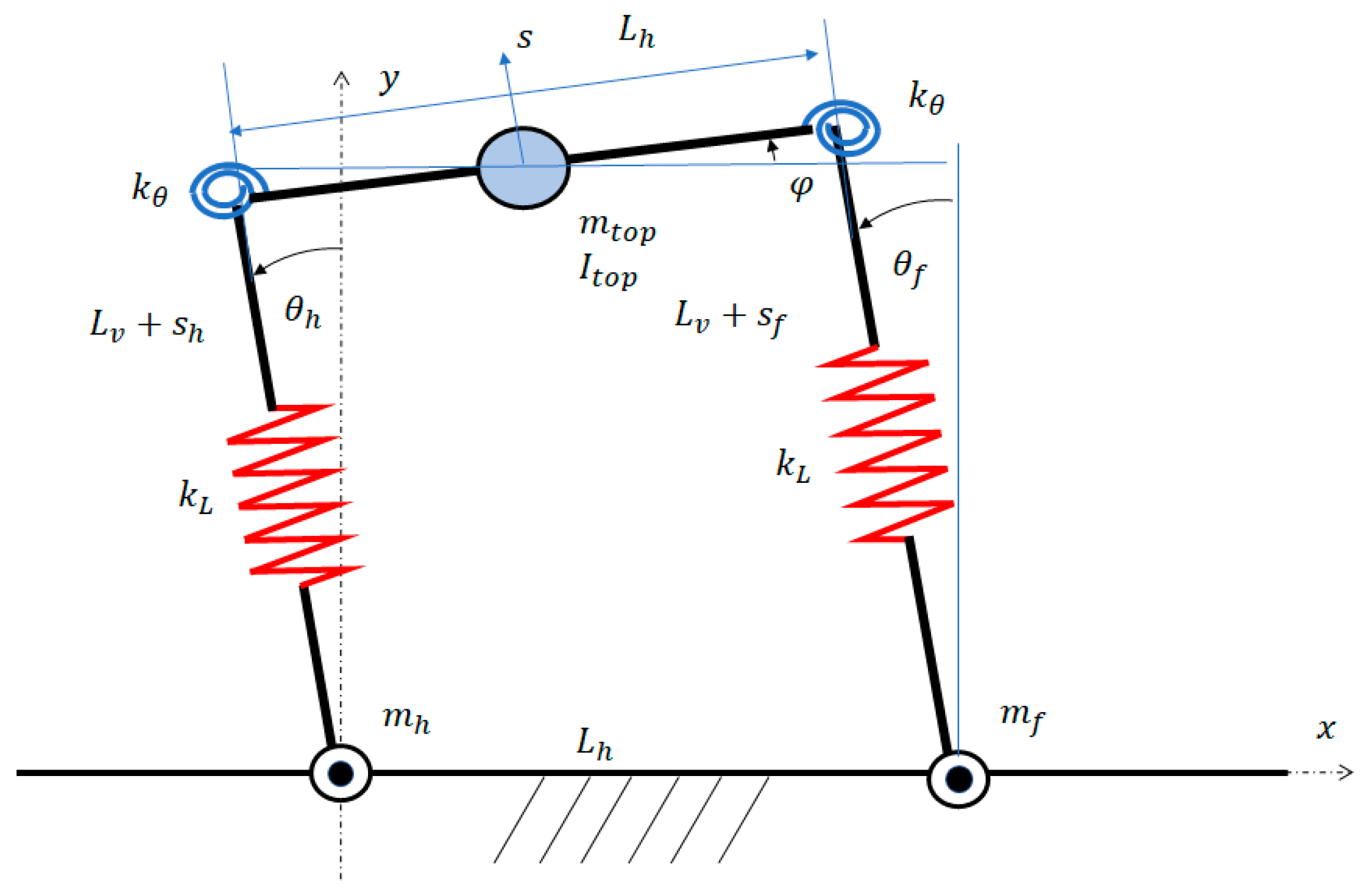
According to the previously mentioned assumptions, the proposed model consists of lumped masses connected by elastic elements, as shown in Figure 2. The first of these lumped masses ($m_{top}$) is located in the center of the spine; it represents the motor and spine masses, and a share (50%) of leg masses. The moment of inertia $I_{top}$ is the moment of inertia about the center of the spine. The other two masses ($m_f$ and $m_h$) represent the masses of the front and hind feet and a share (50%) of leg masses. They are still. The length of the spine is denoted by $L_h$, the lengths of the front and hind legs are $L_v$, and the angles between the legs and the vertical direction are ${\theta }_f$ and ${\theta }_h$, respectively. The spine and the legs are connected by torsional springs with stiffness $k_{\theta }$. The legs of the robot are modeled as linear springs with stiffness $k_L$.

When the robot is in contact with the ground and friction prevents any tangential motion between the feet and the ground itself, the legs with the spine and the ground make up a flexible four-bar linkage [40]. Figure 2 shows that the configuration of this linkage depends on five variables: the rotations of the two legs with respect to the $y$-axis $\left({\theta }_h, {\theta }_f\right)$, the rotation of the spine with respect to the $x$-axis ($\phi$), and the lengths of the two legs ($L_v+s_h$, $L_v+s_f$), in which $s_h$ and $s_f$ are length variations due to axial deformability.

Actually, these five parameters are linked by the closure equation of the linkage and only three variables are independent. The components of the closure equation in $x$ and $y$ directions are:

$$\left(L_v+s_h\right)\cos \left({\theta }_h+\frac{\pi }{2}\right)+L_{h}cos\left(\phi \right)-\left(L_v+s_f\right)\cos \left({\theta }_f+\frac{\pi }{2}\right)-L_h=0$$

(1)

$$\left(L_v+s_h\right)\sin \left({\theta }_h+\frac{\pi }{2}\right)+L_{h}sin\left(\phi \right)-\left(L_v+s_f\right)\sin \left({\theta }_f+\frac{\pi }{2}\right)=0$$

(2)

and expanding the trigonometric functions:

$$-\left(L_v+s_h\right)\sin \left({\theta }_h\right)+L_{h}cos\left(\phi \right)+\left(L_v+s_f\right)\sin \left({\theta }_f\right)-L_h=0$$

(3)

$$\left(L_v+s_h\right)\cos \left({\theta }_h\right)+L_{h}sin\left(\phi \right)-\left(L_v+s_f\right)\cos \left({\theta }_f\right)=0$$

(4)

Since the variations in the lengths and angles caused by robot elastic deformation are small, these equations can be linearized around the reference configuration:

$$-L_v{\theta }_h+L_h+L_v{\theta }_f-L_h=0$$

(5)

$$L_v+s_h+L_h\phi -L_v-s_f=0$$

(6)

Equation (5) leads to:

$${\theta }_h={\theta }_f\equiv \theta$$

(7)

Coordinate $\theta$ is associated with the torsion angle of the linkage. Equation (6) links three variables ($s_h$, $s_f$, and $\phi$). Therefore, two independent parameters can be chosen:

$$\frac{s_f-s_h}{L_h}=\phi$$

(8)

$$\frac{s_h+s_f}{2}=s$$

(9)

Variable $s$ represents the heave of the spine along the leg’s direction, which may be tilted by angle $\theta$. Variables $\theta$, $s$, and $\phi$ are the generalized coordinates describing the motion of the deformable linkage. The equations of the vibrations of the robot can be derived with the Lagrange’s method [41]:

$$\frac{d}{dt}\left(\frac{\partial L}{\partial {\dot{q}}_k}\right)-\frac{\partial L}{\partial q_k}=Q_k k=\mathrm{1..3}$$

(10)

in which $q_1=\theta$, $q_2=s$, and $q_3=\phi$. The Lagrangian components of forces ($Q_k)$ include the forces generated by the eccentric mass and are zero when free vibrations are considered. $L$ is the Lagrange’s function (which is the difference between kinetic and potential energy).

The components of the velocity of the system’s center of mass can be calculated by neglecting second order terms:

$$\begin{array}{cc}{\dot{x}}_G=-L_v\dot{\theta }& {\dot{y}}_G=\dot{s}\end{array}$$

(11)

The kinetic energy according to König’s theorem is:

$$E_k=\frac{1}{2}{m}_{top}\left({\left(-L_v\dot{\theta }\right)}^2+{\dot{s}}^2\right)+\frac{1}{2}{I}_{top}{\dot{\phi }}^2$$

(12)

The potential energy includes the elastic energy related to robot deformation and the gravitational energy:

$$E_p=2\left(\frac{1}{2}{k}_{\theta }{\left(\theta -\phi \right)}^2\right)+\frac{1}{2}{k}_s{\left(s-\frac{L_h}{2}\phi \right)}^2+\frac{1}{2}{k}_s{\left(s+\frac{L_h}{2}\phi \right)}^2+m_{tot}g\left(L_v+s\right)\cos \left(\theta \right)$$

(13)

If a second order approximation is adopted, the potential energy becomes:

$$E_p=k_{\theta }{\left(\theta -\phi \right)}^2+k_s{s}^2+k_{\theta }{\left(\frac{L_h}{2}\phi \right)}^2+m_{tot}g\left(L_v+s\right)-m_{tot}g{L}_v\frac{{\theta }^2}{2}$$

(14)

The expansion of the Lagrange’s equations leads to the equations of the free undamped vibrations of the robot in matrix form:

$$\left[\begin{array}{ccc}{L}_v^2{m}_{top}& 0& 0\\ 0& m_{top}& 0\\ 0& 0& I_{top}\end{array}\right]\left\{\begin{array}{c}\ddot{\theta }\\ \ddot{s}\\ \ddot{\phi }\end{array}\right\}+\left[\begin{array}{ccc}2k_{\theta }-m_{tot}g{L}_v& 0& -2k_{\theta }\\ 0& 2k_s& 0\\ -2k_{\theta }& 0& 2k_{\theta }+0.5L_h^2{k}_s\end{array}\right]\left\{\begin{array}{c}\theta \\ s\\ \phi \end{array}\right\}=\left\{\begin{array}{c}0\\ m_{tot}g\\ 0\end{array}\right\}$$

(15)

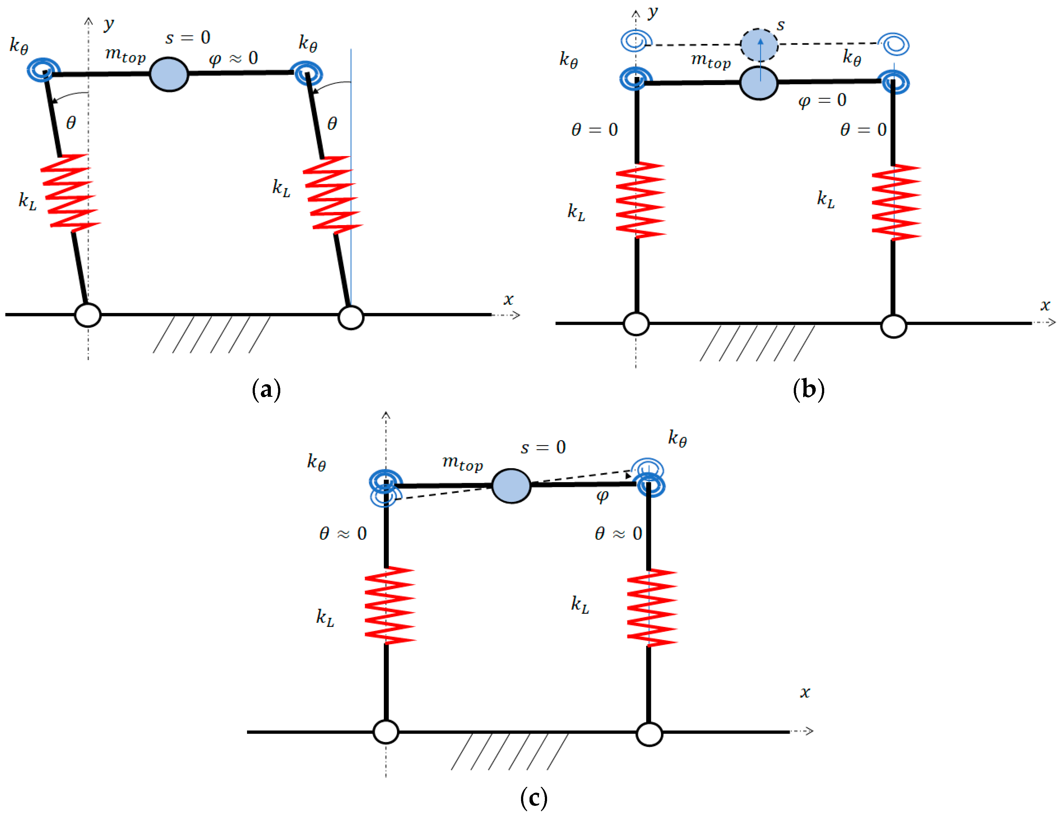
The analysis of these equations shows that the translational vibration of the top mass along the direction of the legs, which is due to axial compliance, is completely uncoupled from the rotational vibrations involving coordinates $\theta$ and $\phi$. There is a coupling between rotation $\theta$ (torsion rotation of the linkage) and rotation $\phi$ (pitch rotation of the spine). Actually, with the values of $k_s$ and $k_{\theta }$ corresponding to straight legs, the stiffness of the legs ($0.5 L_h^2{k}_s$) that opposes to the pitch rotation of the spine ($\phi$) is very large and rotation $\phi$ is very small. Therefore, the modes of vibration corresponding to the torsion rotation of the linkage ($\theta$) and pitch rotation of the spine ($\phi$) are nearly uncoupled. Figure 3 shows the modes of vibration of the robot walking on the ground.

Since the three modes are nearly uncoupled, simplified equations can be used to estimate the natural frequencies of the vibrational modes:

$${\omega }_{\theta }=\sqrt{\frac{2k_{\theta }-m_{top}g{L}_v}{L_v^2{m}_{top}}}$$

(16)

$${\omega }_s=\sqrt{\frac{2k_L}{m_{top}}}$$

(17)

$${\omega }_{\phi }=\sqrt{\frac{0.5L_h^2{k}_s}{I_{top}}}$$

(18)

The equations for the torsion and heave frequencies are equal to the ones reported in Reference [25]. With the mass and stiffness properties of the present robot ($k_{\theta }$= 0.17 Nm/rad and $k_L$= 4.3$\times$10⁶ N/m), the difference between exact and approximate values of ${\omega }_{\theta }$ and ${\omega }_{\phi }$ is less than 0.1%. The natural frequencies of the three modes are: ${\omega }_{\theta }$ = 108.3 rad/s, ${\omega }_s$ = 38,487.3 rad/s, and ${\omega }_{\phi }$ = 72,654.4 rad/s.

Since the torsion mode has the lowest natural frequency, the eccentric mass can excite this mode more easily than the other modes.

3.2. Modes of Vibration Due to Floating

According to the Archimedes’ principle, a floating body reaches an equilibrium position when the weight of the displaced water is equal to the weight of the body. The robot walking on the water reaches an equilibrium position when:

$$m_{tot}g=2{\rho }_w\mathrm{g}\nabla$$

(19)

in which $m_{tot}$ is the total mass of the robot, ${\rho }_w$ is the density of water, and $\nabla$ is the water volume displaced by each floating foot, which corresponds to a specific draft.

If an initial perturbation causes small variations in the drafts of the floating feet, the vertical buoyancy forces become:

$$F_{f,y,b}={\rho }_w\mathrm{g}\nabla -{\rho }_w\mathrm{gA}{s}_f$$

(20)

$$F_{h,y,b}={\rho }_w\mathrm{g}\nabla -{\rho }_w\mathrm{gA}{s}_h$$

(21)

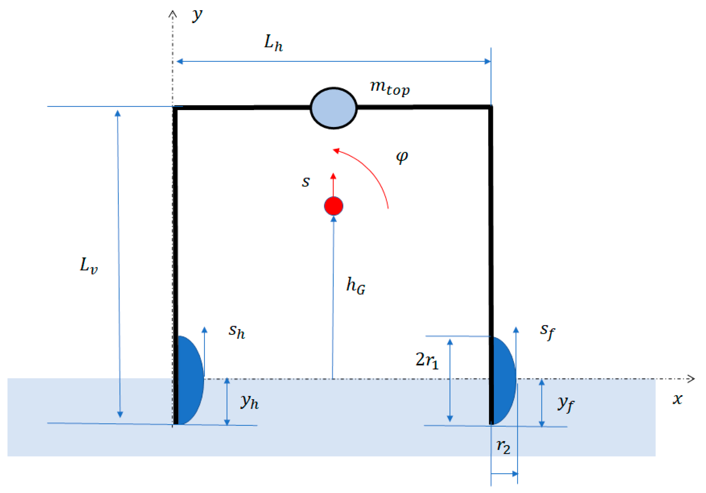
in which $F_{f,y,b}$ and $F_{h,y,b}$ are the buoyancy forces on the front and hind foot, respectively, and $s_f$ and $s_h$ are the small vertical displacements of the floating feet, which are represented in Figure 4. $A$ is the water plane area [42] of each foot. Since small oscillations are considered, the water plane area can be considered constant: $A\approx r_2{L}_p$, in which $L_p$ is the axial length of the foot.

The second terms in Equations (20) and (21), which are linear on $s_f$ and $s_h$, are the restoring forces exerted by the water on the feet. The corresponding equivalent stiffness is ${\rho }_w\mathrm{g}A$.

When an object vibrates on the water, the added mass is another important phenomenon that has to be considered. A share of the water surrounding the object vibrates with the object itself, adds to the mass of the object, and reduces the natural frequency of free vibrations. The added mass has been widely studied in the fields of fluid-dynamics, maritime, and naval engineering [42], adopting experimental [43] and numerical methods [44]. Since the feet of the robot are floating, the specific added mass coefficient presented in Reference [43] has been adopted to calculate the added mass of each foot:

$$m_{add}=c_V\frac{1}{2}{\rho }_w\pi b_e{}^2$$

(22)

in which $b_e$ is the half-beam of the floating body and $c_V=1.4$ is the added mass coefficient.

In this study, the amphibious robot is considered as a rigid beam with distributed mass properties and some lumped masses (the mass of the motor with the eccentric mass, and the masses of the feet). Structural deformability and damping are neglected. With the previously mentioned assumptions, the dynamic system has 2 degrees of freedom: vertical displacement $s$ of the center of mass and rotation $\phi$ about the center of mass (see Figure 4).

The equations of motion are derived with the Lagrange’s method. Some kinematic calculations are first performed in order to calculate the vertical displacements of the feet $(s_f$ and $s_h)$ as functions of $s$ and $\phi$:

$$s_f=s+\frac{L_h}{2}\sin \left(\phi \right)+h_G\left(1-\cos \phi \right)$$

(23)

$$s_h=s-\frac{L_h}{2}\sin \left(\phi \right)+h_G\left(1-\cos \phi \right)$$

(24)

in which $h_G$ is the height of the center of mass with respect to the water level (see Figure 4). Expanding the trigonometric functions in Taylor’s series, the following equations hold:

$$s_f=s+\frac{L_h}{2}\phi +h_G\frac{{\phi }^2}{2}$$

(25)

$$s_h=s-\frac{L_h}{2}\phi +h_G\frac{{\phi }^2}{2}$$

(26)

The Lagrangian components of the buoyancy forces are:

$$Q_s=\left({\rho }_w\mathrm{g}\nabla -{\rho }_w\mathrm{gA}{s}_f\right)\frac{\partial s_f}{\partial s}+\left({\rho }_w\mathrm{g}\nabla -{\rho }_w\mathrm{gA}{s}_h\right)\frac{\partial s_h}{\partial s}$$

(27)

$$Q_{\phi }=\left({\rho }_w\mathrm{g}\nabla -{\rho }_w\mathrm{gA}{s}_f\right)\frac{\partial s_f}{\partial \phi }+\left({\rho }_w\mathrm{g}\nabla -{\rho }_w\mathrm{gA}{s}_h\right)\frac{\partial s_h}{\partial \phi }$$

(28)

It is worth noting that second orders expressions of $s_f$ and $s_h$ are needed to take into account the constant term (${\rho }_w\mathrm{g}\nabla$) of buoyancy forces.

The kinetic energy of the system is:

$$E_k=\frac{1}{2}\left(m_{tot}+2m_{add}\right){\dot{s}}^2+\frac{1}{2}\left(I_{tot}+2I_{add}\right){\dot{\phi }}^2$$

(29)

in which $I_{tot}$ is the moment of inertia of the rigid body about the global center of mass. $I_{add}$ is the contribution of each added mass to the moment of inertia:

$$I_{add}=m_{add}\left({\left(\frac{L_h}{2}\right)}^2+h_G{}^2\right)$$

(30)

Since the buoyancy forces have been already taken into account, the potential energy only depends on the gravity force of the robot:

$$E_p=m_{tot}g\left(h_{GR}+s\right)$$

(31)

in which $h_{GR}$ is the vertical position of the center of mass of the robot.

The application of the Lagrange’s method leads to the following equations of motion of the floating robot.

$$\left(m_{tot}+2m_{add}\right)\ddot{s}+m_{tot}g=2{\rho }_w\mathrm{g}\nabla -2{\rho }_w\mathrm{gAs}$$

(32)

$$\left(I_{tot}+2I_{add}\right)\ddot{\phi }=2{\rho }_w\mathrm{g}\nabla h_G\phi -2{\rho }_w\mathrm{gA}{\left(\frac{L_h}{2}\right)}^2\phi$$

(33)

Making use of the static equilibrium condition in Equation (19), the equations of motion become:

$$\left(m_{tot}+2m_{add}\right)\ddot{s}+2{\rho }_w\mathrm{gAs}=0$$

(34)

$$\left(I_{tot}+2I_{add}\right)\ddot{\phi }+2{\rho }_w\mathrm{gA}{\left(\frac{L_h}{2}\right)}^2\phi -m_{tot}g{h}_G\phi =0$$

(35)

These equations describe the free vibrations of the floating robot in the $s$ and $\phi$ directions. Since they are uncoupled, the natural frequencies of the heave ($s$) and pitch ($\phi$) modes of vibration can be simply calculated:

$${\omega }_s=\sqrt{\frac{2{\rho }_w\mathrm{gA}}{m_{tot}+2m_{add}}}$$

(36)

$${\omega }_{\phi }=\sqrt{\frac{2{\rho }_w\mathrm{gA}{\left(\frac{L_h}{2}\right)}^2-m_{tot}g{h}_G}{I_{tot}+2I_{add}}}$$

(37)

With the mass properties and the buoyancy characteristics of the robot, the two natural frequencies result in ${\omega }_s$= 34.2 rad/s and ${\omega }_{\phi }$= 28.8 rad/s.

The highest of these natural frequencies is by far lower than the lowest natural frequency of the structural modes (108.3 rad/s). Therefore, the structural modes of vibrations, which are important in terrestrial locomotion [23,25], are negligible in an aquatic locomotion. The model for the study of aquatic locomotion can be thus developed neglecting the structural deformation of the robot.

4. Aquatic Locomotion Model

In this section, a multibody numerical model of the amphibious robot during locomotion in water is presented and discussed. The dynamic model is developed using Working Model (WM) 2D, and the numerical and experimental locomotion speed for different angular velocities of the rotating mass will be compared. This model will help to understand and discuss the locomotion principle in the water.

The WM model, which has been built using the geometrical and inertial parameters of Table 1, and the interaction forces of feet with the water are presented in Figure 5. A planar motion of the robot is assumed, and the frame of the robot is modeled as a rigid body, which is reasonable due to the high frequencies of the structural modes, the low interaction forces with the water, and the low locomotion speed.

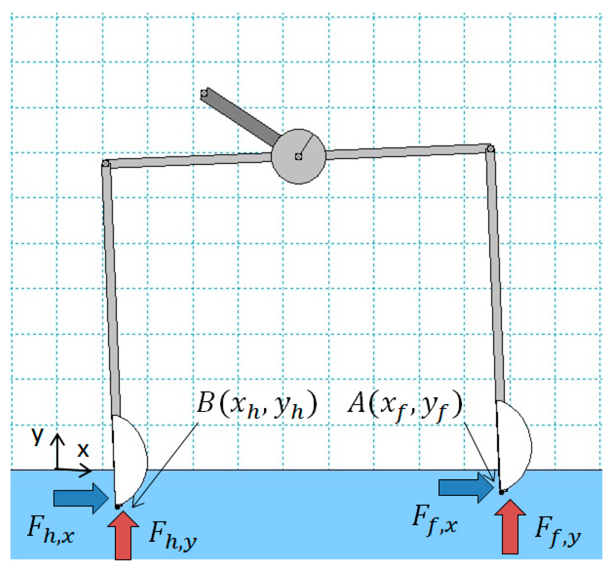
The horizontal force on the front and hind foot ($F_{f,x}$ and $F_{h,x}$, respectively) is mainly due to drag, which is related to the front and hind foot speed along the $x$-axis (${\dot{x}}_f$ and ${\dot{x}}_h$, respectively), but there is also a small lift force that arises when the foot profile moves vertically in the water. The following equations hold:

$$\begin{gathered} F_{f,x}=\frac{1}{2}{\rho }_w{c}_{x,f}{L}_p{y}_f{\dot{x}}_f{}^2+F_{f,l},\mathrm{if}{\dot{x}}_f\ge 0 \\ {F}_{f,x}=-\frac{1}{2}{\rho }_w{c}_{x,b}{L}_p{y}_f{\dot{x}}_f{}^2+F_{f,l},\mathrm{if}{\dot{x}}_f<0 \\ {F}_{f,x}=0,\mathrm{if}{y}_f\ge 0 \end{gathered}$$

(38)

$$\begin{gathered} F_{h,x}=\frac{1}{2}{\rho }_w{c}_{x,f}{L}_p{y}_h{\dot{x}}_h{}^2+F_{h,l},\mathrm{if}{\dot{x}}_h\ge 0 \\ {F}_{h,x}=-\frac{1}{2}{\rho }_w{c}_{x,b}{L}_p{y}_h{\dot{x}}_h{}^2+F_{h,l},\mathrm{if}{\dot{x}}_h<0 \\ {F}_{h,x}=0,\mathrm{if}{y}_h\ge 0 \end{gathered}$$

(39)

$$\begin{gathered} F_{f,l}=\frac{1}{2}{\rho }_w{c}_l{L}_p{r}_2{d}_f{\dot{y}}_f{}^2 \\ {F}_{h,l}=\frac{1}{2}{\rho }_w{c}_l{L}_p{r}_2{d}_h{\dot{y}}_h{}^2 \end{gathered}$$

(40)

In Equations (38) and (39), ${\rho }_w$ is the density of water, $c_{x,f}$ and $c_{x,b}$ are the drag coefficients in the forward and backward directions along the $x$-axis, respectively, and $y_f$ and $y_h$ are the vertical positions of the front and hind foot, so that $\left|L_p{y}_f\right|$ and $\left|L_p{y}_h\right|$ are the areas (subject to drag forces) of the submerged part of the front and hind foot, respectively. In Equation (40), $F_{f,l}$ and $F_{h,l}$ are the lift forces on the front and hind foot, respectively, $c_l$ is the lift coefficient of the foot subject to a vertical flow, $d_f$ and $d_h$ are the ratio of the submerged length of the front and hind foot with respect to the total foot length (2$r_1$), respectively, and ${\dot{y}}_f$ and ${\dot{y}}_h$ are the front and hind foot speed along the $y$-axis, respectively. As indicated in Equations (38) and (39), the drag forces are always opposite of the foot speed (usually $y_h <0$, i.e., the foot is partially submerged). As indicated in Equations (38) and (39), the horizontal force is null if the foot is completely out of water.

The vertical force on the front and hind foot ($F_{f,y}$ and $F_{h,y}$, respectively) is composed of two terms:

$$\begin{gathered} F_{f,y}=F_{f,y,b}+F_{f,y,d} \\ {F}_{h,y}=F_{h,y,b}+F_{h,y,d} \end{gathered}$$

(41)

where $F_{f,y,b}$ and $F_{h,y,b}$ are the buoyancy forces on the front and hind foot, respectively, and $F_{f,y,d}$ and $F_{h,y,d}$ are the vertical drag forces on the front and hind foot, respectively.

The buoyancy forces on each foot can be modeled as in Section 3.2:

$$\begin{gathered} F_{f,y,b}=-{\rho }_w\mathrm{g}{L}_p{r}_{2,eq}{y}_f \\ {F}_{f,y,b}=0,\mathrm{if}{y}_f\ge 0 \end{gathered}$$

(42)

$$\begin{gathered} F_{h,\mathrm{y},\mathrm{b}}=-{\rho }_w\mathrm{g}{L}_p{r}_{2,eq}{y}_h \\ {F}_{h,\mathrm{y},\mathrm{b}}=0,\mathrm{if}{y}_h\ge 0 \end{gathered}$$

(43)

where $\mathrm{g}$ is the acceleration of gravity, and $r_{2,eq}=\frac{\pi r_2}{4}$ is the width of an equivalent rectangular cuboid with the same length ($L_p$), height ($2r_1$), and volume ($2r_1{r}_{2,eq}{L}_p=\frac{1}{2}\pi r_1{r}_2{L}_p$) of the real foot. This is an approximation that allows to model the buoyancy force on each foot as a linear function of $y_f$ (or $y_h$). Equations (42) and (43) show that the buoyancy force is null if the foot is completely out of the water.

The vertical drag force on the front and hind foot, which is due to the front and hind foot speed along the $y$-axis (${\dot{y}}_f$ and ${\dot{y}}_h$, respectively), can be modeled as:

$$\begin{gathered} F_{f,y,d}=-\frac{1}{2}{\rho }_w{c}_{y,f}{L}_p{r}_{2,eq}{\dot{y}}_f{}^2,\mathrm{if}{\dot{y}}_f\ge 0 \\ {F}_{f,y,d}=\frac{1}{2}{\rho }_w{c}_{y,b}{L}_p{r}_{2,eq}{\dot{y}}_f{}^2,\mathrm{if}{\dot{y}}_f<0 \\ {F}_{f,y,d}=0,\mathrm{if}{y}_f\ge 0 \end{gathered}$$

(44)

$$\begin{gathered} F_{h,y,d}=-\frac{1}{2}{\rho }_w{c}_{y,f}{L}_p{r}_{2,eq}{\dot{y}}_h{}^2,\mathrm{if}{\dot{y}}_h\ge 0 \\ {F}_{h,y,d}=\frac{1}{2}{\rho }_w{c}_{y,b}{L}_p{r}_{2,eq}{\dot{y}}_h{}^2,\mathrm{if}{\dot{y}}_h<0 \\ {F}_{h,y,d}=0,\mathrm{if}{y}_h\ge 0 \end{gathered}$$

(45)

where $c_{y,f}$ and $c_{y,b}$ are the drag coefficients in the forward and backward directions along the $y$-axis, respectively, and $L_p{r}_{2,eq}$ is the equivalent area of the cross section (orthogonal to the $y$-axis) of the submerged part of the foot. As indicated in Equations (44) and (45), the drag forces always have the opposite sign with respect to the foot speed, and are null if the foot is completely out of the water.

Due to the shape of the foot, $c_{x,f}$ and $c_{x,b}$ have different values. In the dynamic simulations, it is assumed [45,46,47]: $c_{x,f}$ = 1.15, $c_{x,b}$ = 2.15, $c_{y,f}$ = 0.8, $c_{y,b}$ = 0.8, and $c_l$ = 0.045.

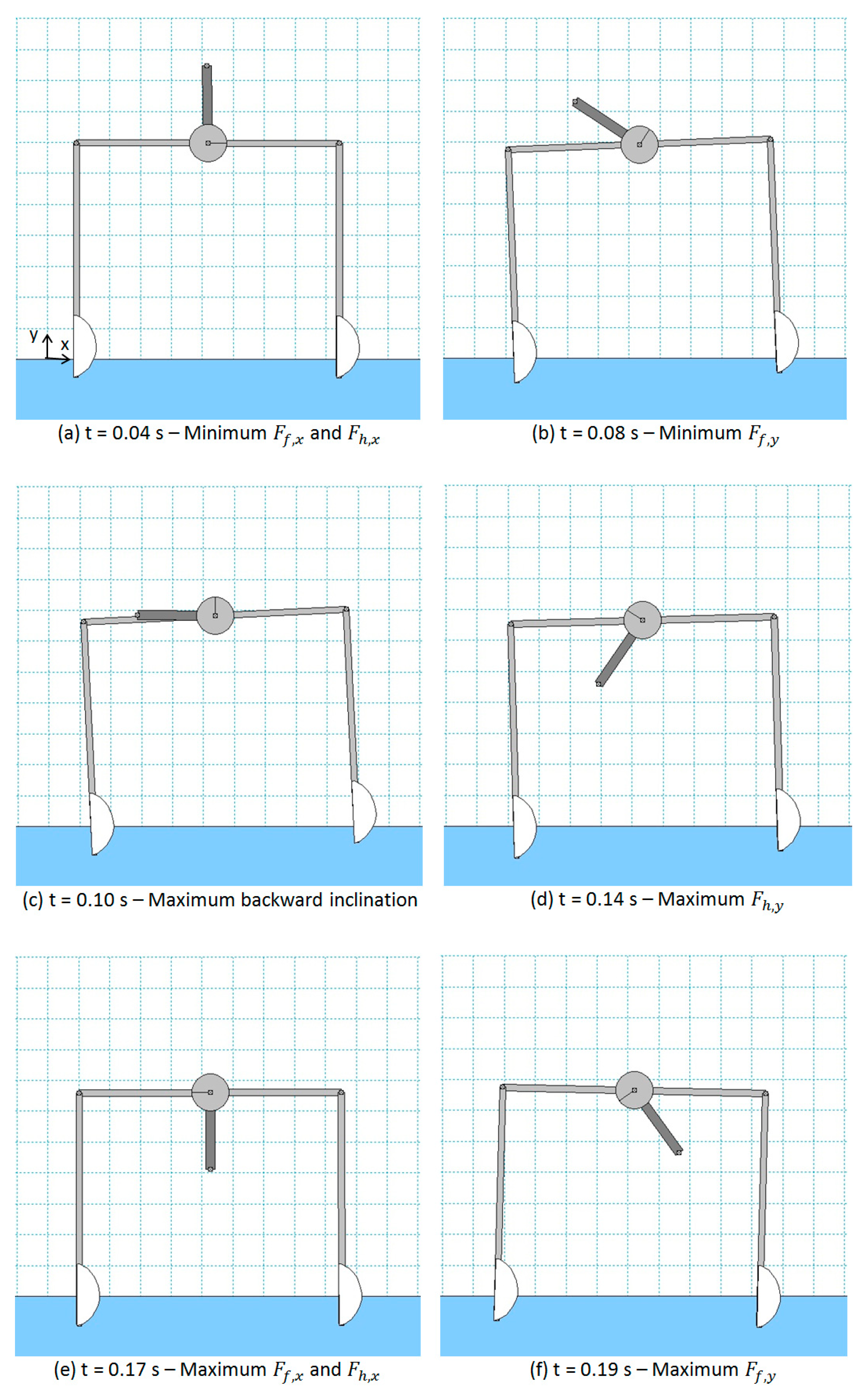
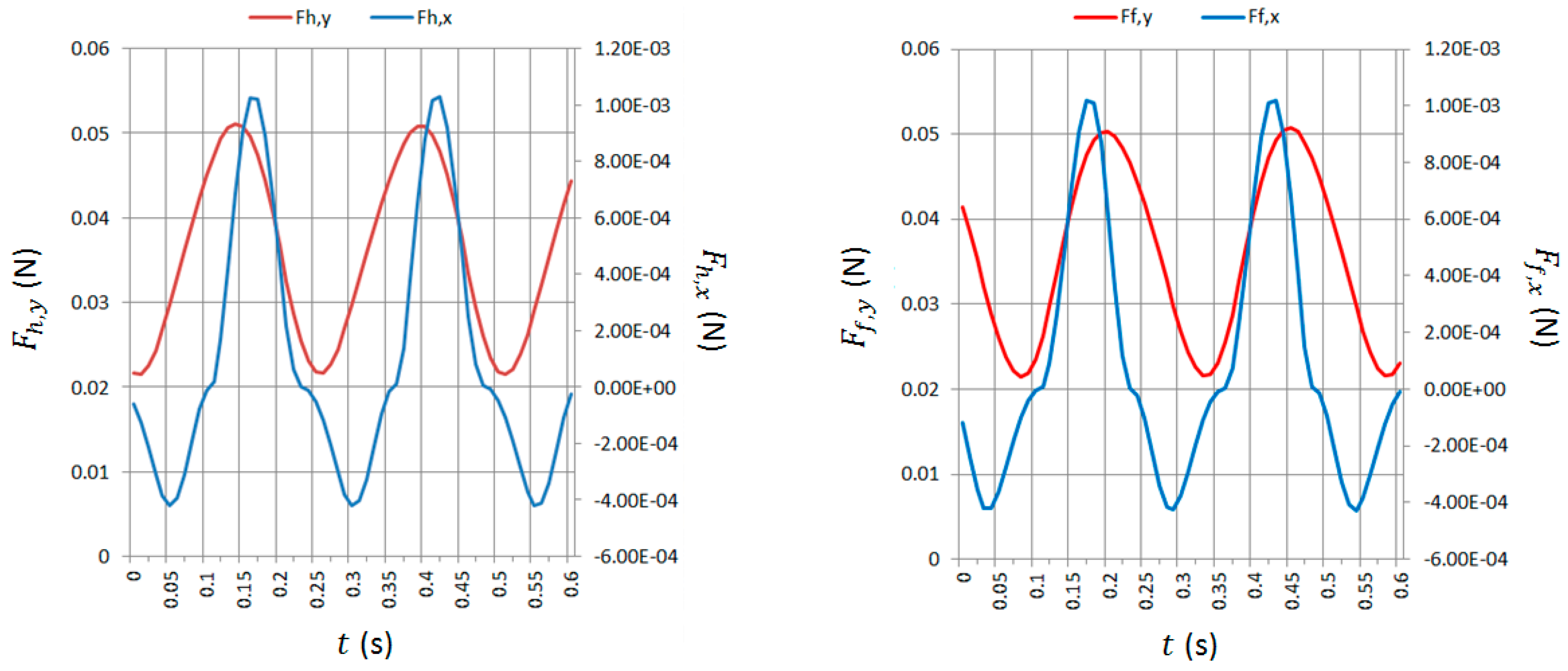
In Figure 6, a sequence of screenshots is presented, which have been derived from a simulation performed with angular velocity of the rotating mass $\omega$ = 24 rad/s (counter-clockwise). The configurations reported in Figure 6 match well with the ones observed during the experimental tests. After an initial transient, the motion of the robot is periodic. Thus, the same motion (and the related sequence of configurations) is repeated every time period $T=\frac{2\pi }{\omega }$. In Figure 7, the forces on the front ($F_{f,x}$, $F_{f,y}$) and hind foot ($F_{h,x}$, $F_{h,y}$) as a function of time ($t$) are reported for a couple of cycles. It can be noticed that $F_{f,x}$ and $F_{h,x}$ have a very similar profile and are almost in phase. In addition, $F_{f,y}$ and $F_{h,y}$ have a similar profile, but $F_{f,y}$ is shifted to about 0.065 s (which corresponds to a phase shift of about 90 deg) with respect to $F_{h,y}$, since the robot oscillates backward and forward (see Figure 6) as it advances.

From the analysis of Figure 6 and Figure 7, the following considerations can be done. In the screenshot (a), the rotating link (carrying the eccentric mass) is vertical and pointing upwards and the feet of the robot are moving forward. In this configuration, the minimum (directed backwards and largest in modulus) horizontal drag forces are applied to the feet of the robot (see $F_{f,x}$ and $F_{h,x}$ at $t$ = 0.04 s in Figure 7). Moreover, in this configuration, the centrifugal force due to the rotating mass is pointing upwards, so the submerged part of the feet is less than in the static equilibrium configuration (rotating mass not moving).

In the screenshot (e) (which is a dual configuration with respect to (a)), the rotating link is vertical and pointing downward and the feet of the robot are moving backward. In this configuration, the maximum (positive, i.e., directed forward) horizontal drag forces are applied to the feet of the robot (see $F_{f,x}$ and $F_{h,x}$ at $t$ = 0.17 s in Figure 7). In this configuration, the centrifugal force due to the rotating mass is pointing downward, so the submerged part of the feet is more than in the static equilibrium configuration. Therefore, the submerged area of the feet subject to horizontal drag forces is higher than in (a), and this contributes to have a higher value (in modulus) of the forward force with respect to the backward force related to (a). Nevertheless, the main reason why the absolute value of the maximum forward force (for each foot) is higher than the absolute value of the minimum (backward) force is because $c_{x,b}>c_{x,f}$.

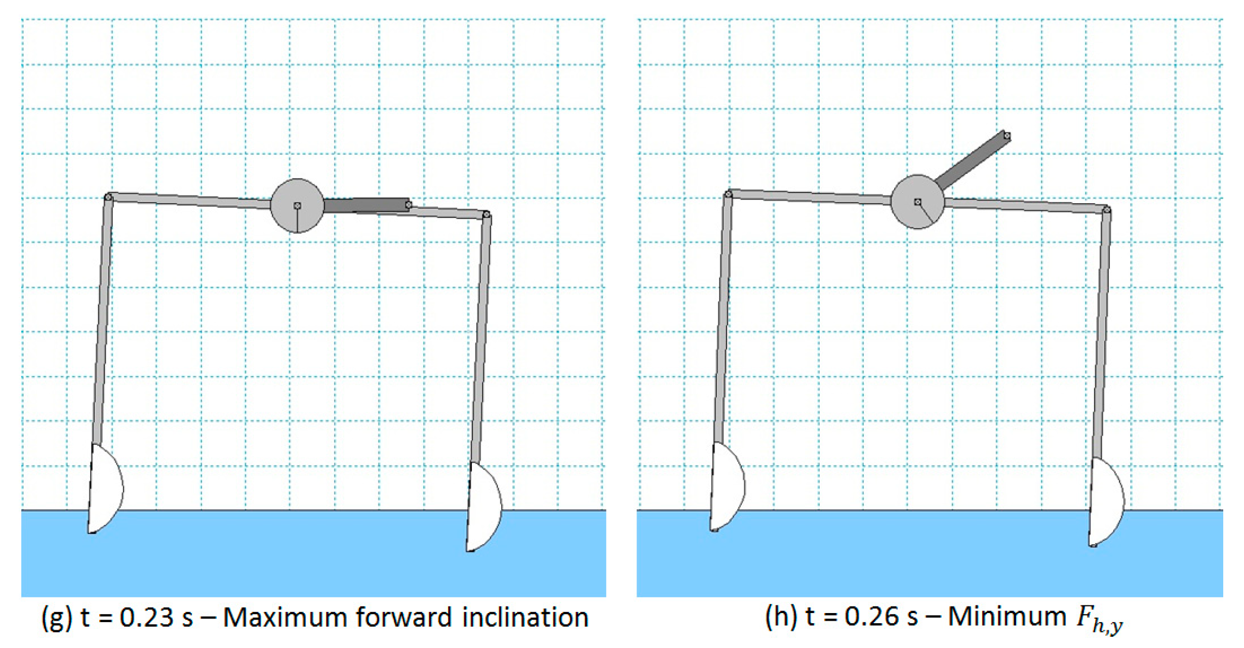
Similarly, in all the other configurations, the robot motion is dominated by the corresponding direction of the centrifugal force generated by the rotating mass. In particular, in configuration (b), the minimum value of $F_{f,y}$ is reached, as it can be verified in Figure 7 for $t$ = 0.08 s and, indeed, the direction of the centrifugal force (i.e., the direction of the rotating link) is such that it reduces the vertical load on the front foot (and, thus, reduce the buoyancy force and $F_{f,y}$). In configuration (c), the maximum backward inclination of the robot (about −2.5 deg) is reached and the centrifugal force is horizontal so that the maximum destabilizing torque on the robot is achieved. In configuration (d), the maximum value of $F_{h,y}$ is reached, as it can be verified in Figure 7 for $\mathrm{t}$ = 0.14 s, and the direction of the centrifugal force (i.e., the direction of the rotating link) is such that it increases the vertical load on the hind foot (and, thus, increases the buoyancy force and $F_{h,y}$).

Exactly the same considerations can be done for configurations (f), (g), and (h), in which the centrifugal force makes the vertical load on the front foot increase (together with the related buoyancy force), makes the robot achieve its maximum forward inclination (about −2.5 deg), and makes $F_{h,y}$ (and the related buoyancy force) reach its minimum value, respectively.

It can be concluded that the main reason for robot net forward motion is that $c_{x,b}>c_{x,f}$ due to the asymmetric shape of the feet. In the periodic forward-backward motion of the feet with respect to the water (due to the centrifugal force of the eccentric mass that pulls forward and backward the robot), a positive integral force due to horizontal drag forces allows the robot to advance. This can be easily verified looking at the profile of $F_{f,x}$ and $F_{h,x}$ in Figure 7. The area of the positive part of the plot is higher than the area of the negative part of the plot for both feet. This phenomenon is similar to the one exploited in vibration conveying [48], in which the inclination of the inertia force caused by vibrations increases the static friction force in a direction and decreases the static friction force in the opposite direction.

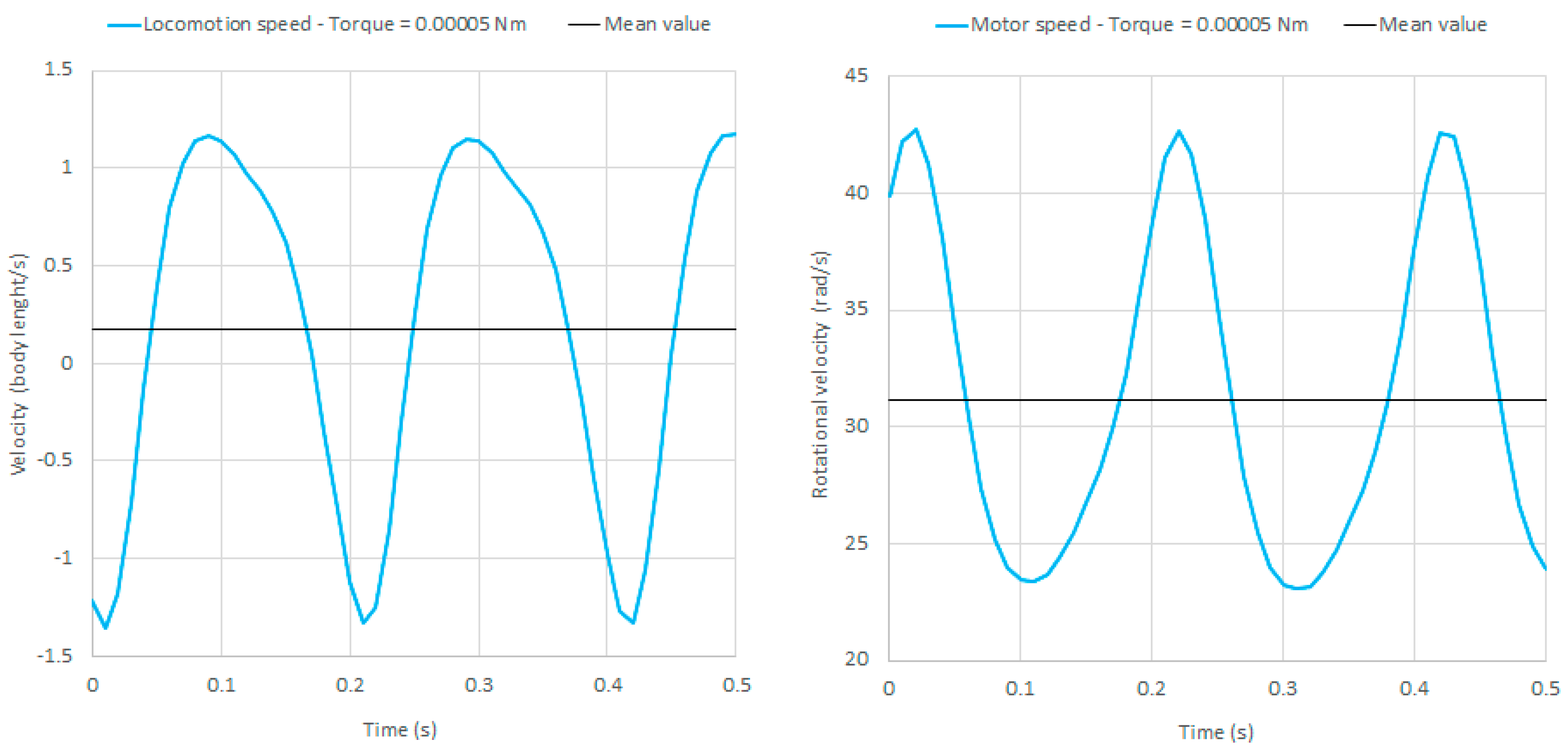
The dynamic behavior of the robot using a constant motor torque as an input has also been investigated. In particular, simulations have been carried out with torques (directed counterclockwise) from 0.00001 Nm to 0.01 Nm. For low torque values, i.e., from 0.00001 to 0.00004 Nm, the torque is not sufficient to rotate the eccentric mass. For torque values between 0.00004 and 0.0005 Nm, a stable periodic locomotion is obtained, after an initial transient. The locomotion speed, expressed in body length/mm (the body length is $L_h$ = 85 mm), the motor speed, and their mean values (0.173 body length/s and 31 rad/s, respectively) are reported in Figure 8 for an input torque of 0.00005 Nm.

For torque values higher than 0.00005 Nm, the rotating mass is continuously accelerated until the robot reaches a stable periodic locomotion with rotational speeds higher than 200 rad/s, which is not reasonable for this type of robot. For torque values higher than 0.01 Nm, the robot tips over.

It can be concluded that the use of a constant torque as an input allows for a stable locomotion only for motor torques between 0.00004 and 0.00005 Nm. The use of a constant angular velocity as an input is much more reasonable, since it allows us to excite the resonances of the system. Moreover, it is more flexible (since the locomotion speed can be precisely tuned), and it results in higher locomotion speeds, as detailed in Section 5.

5. Experimental Results

During the experiments (see video S1 published as Supplementary Material), the angular velocity of the eccentric mass is controlled by the voltage applied to the DC motor. The aquatic and terrestrial locomotion of the robot is recorded with a high-speed camera while the robot is moving in a 0.7 × 1.5 m aquarium, and the locomotion speed, the rotating mass rotational speed, and the robot foot positions are measured thanks to high-speed camera recordings. The DC motor voltage is increased from 0.8 V to 2.7 V in 0.1 Volt increments.

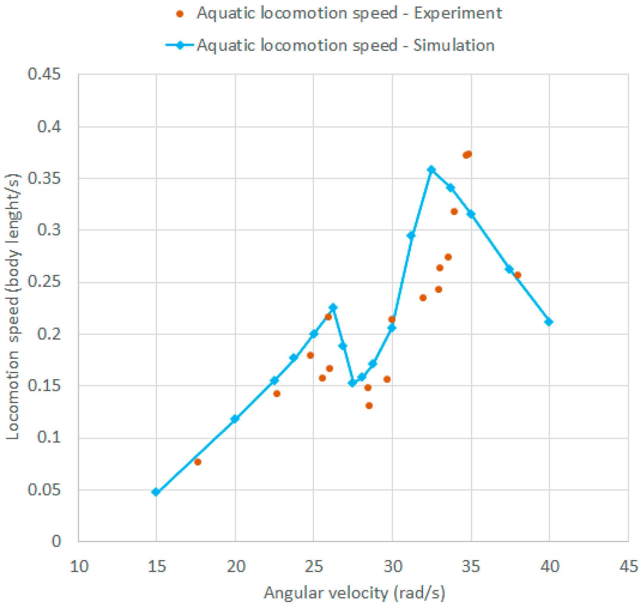
In Figure 9, the experimental and numerical aquatic locomotion speed as a function of $\omega$ (counterclockwise rotation) are overlapped. The numerical curve has been derived using the WM model presented in Section 4. It can be observed that there is good agreement between the resonance frequencies of the numerical and experimental model. A first resonance peak appears at about 26.5 rad/s and a second resonance peak appears at about 33–35 rad/s in both cases. These values are also in good agreement with the resonance frequencies computed with the linear model of Section 3.2 (28.8 rad/s and 34.2 rad/s). Moreover, the numerical and experimental curves are in good agreement and nearly overlapped. For higher values of $\omega$ (>40 rad/s), the numerical model cannot be used due to the increasing importance of the effect of waves generated by the robot (which are observed in the experiments). It is worth noting that the natural frequencies of aquatic locomotion are well below the natural frequencies of the structural modes studied in Section 3.1. Hence, the assumption of rigid robot in the model of aquatic locomotion is consistent with the actual operation of the robot.

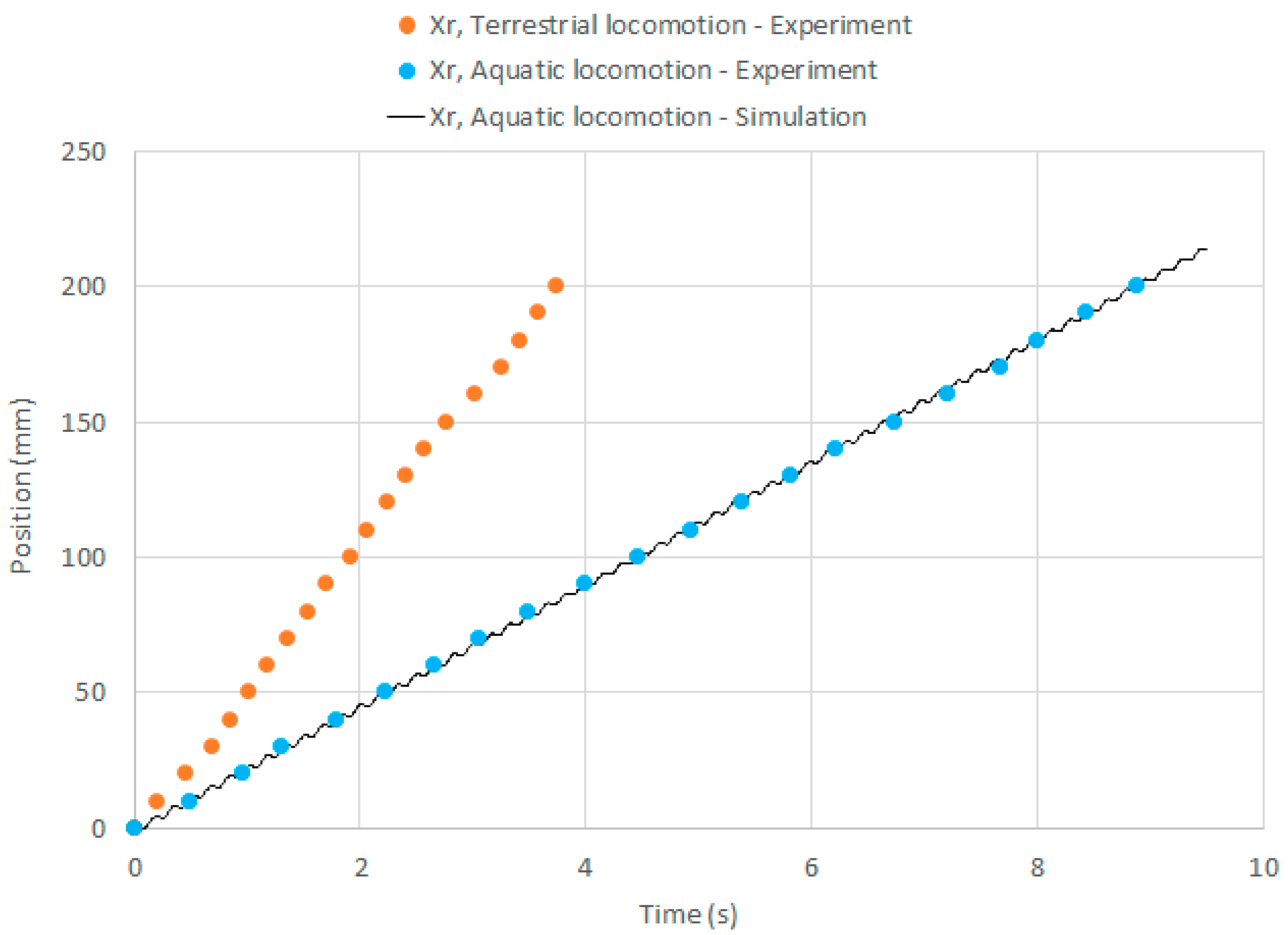
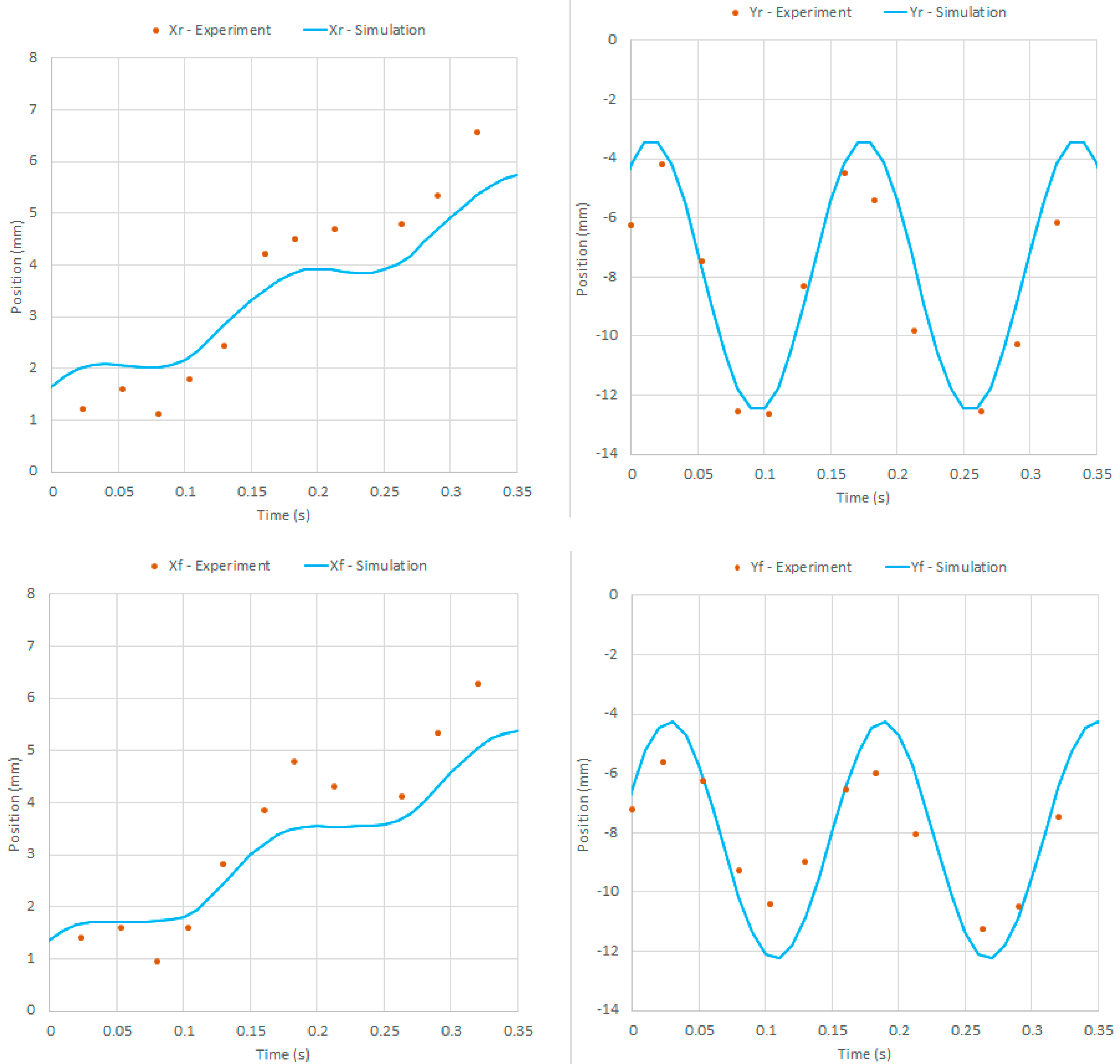
In Figure 10, the displacements of the hind foot are presented both for terrestrial and aquatic locomotion, which have been measured in experiments with $\omega$ = 38 rad/s. The experimental curves are almost linear, and this is related to constant locomotion speeds. In the case of aquatic locomotion, the experimental points are overlapped with the numerical curve, which is almost linear with small local peaks due to the periodic locomotion. The experimental and numerical results are in good agreement. A more detailed comparison between the experimental and numerical positions of the robot feet is depicted in Figure 11 considering a couple of periods of motion. Experimental and numerical data are in good agreement in this time scale as well: the period of the oscillations is the same and the error between the numerical curve and the experimental points is always less than 1.3 mm.

The differences between numerical and experimental data in Figure 9, Figure 10 and Figure 11 are mainly due to all the simplifying assumptions (detailed in Section 4), the disturbance forces related to the electrical cables of the motor, and the effect of the small waves present in the experiment, which are not considered in the numerical model. The overlap between the experimental points and numerical curves could be improved by using computational fluid dynamics to simulate the flow around feet for different relative velocities and angles, or by using experimentally determined drag and lift coefficients. However, these activities are beyond the scope of the present work.

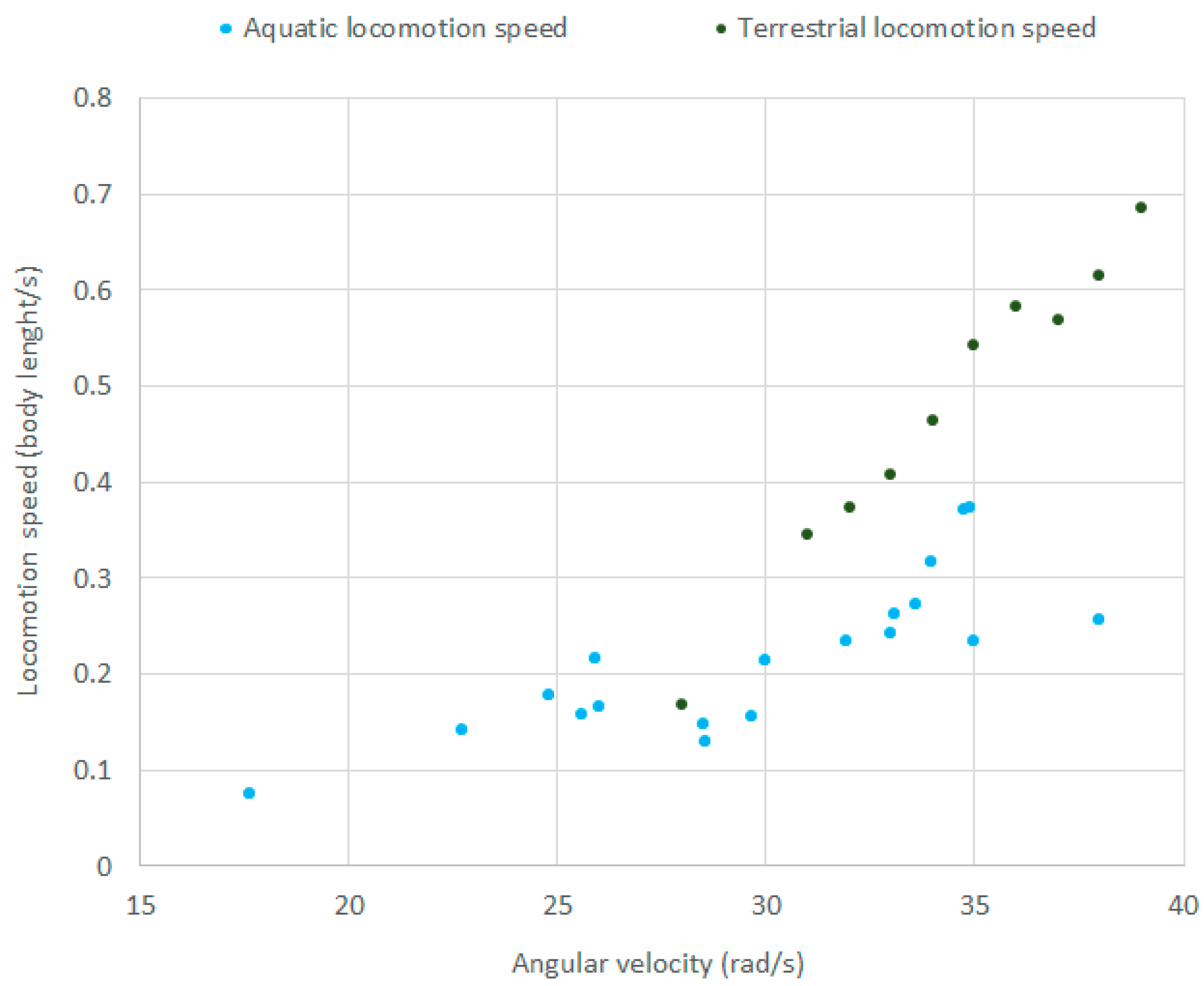
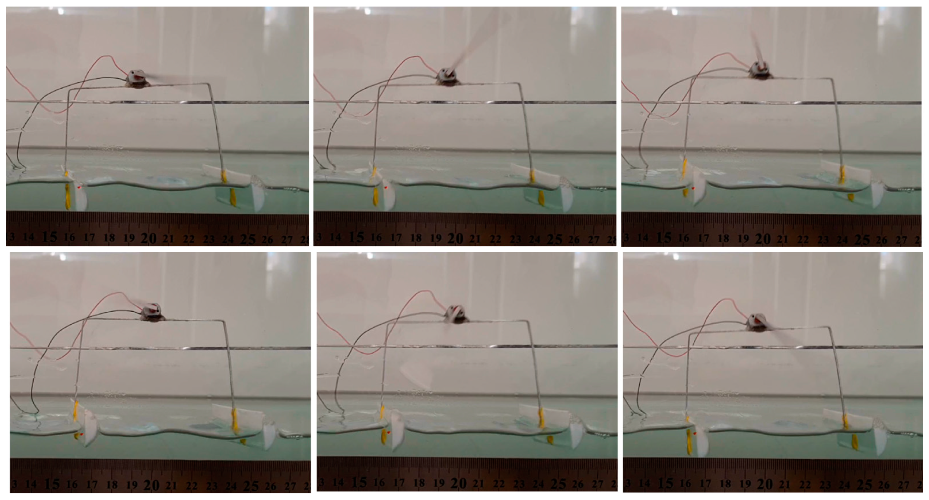
Figure 12 shows both the terrestrial and aquatic locomotion speed as a function of $\omega$, as measured in the experiments. The figure shows that the robot reaches the highest speed on the ground when the eccentric mass rotates at an angular velocity of about 38 rad/s, and it reaches the highest speed on the water when the eccentric mass rotates at an angular velocity of about 35 rad/s, which is in accordance with the resonance peak found with the mathematical and numerical models of Section 3 and Section 4. In Figure 13, a sequence of photos showing an aquatic locomotion test with $\omega$ = 25 rad/s is presented.

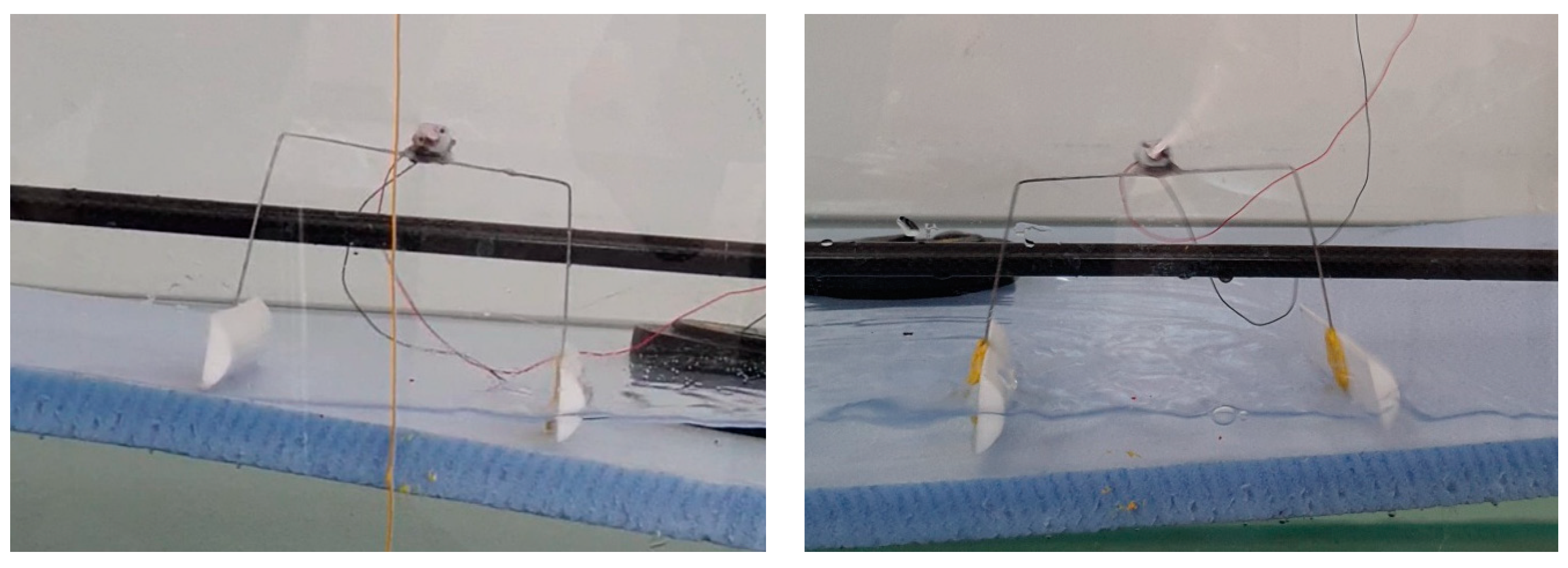
The proposed robot is able to carry out the transition ground-water and vice-versa as shown in Figure 14 and in video S1 (published as Supplementary Material). Even if the ground locomotion is not the focus of the present work, it should be noted that the robot is very robust against big variations in the coefficients of friction (both static and dynamic) of the surface. In the transition water-ground, the feet are wet (which causes a significant decrease in the friction coefficients); nevertheless, the robot is able to successfully perform the transition. The investigation of the effect of friction coefficients in the ground locomotion and in the transition phases will be part of future work.

6. Conclusions

An amphibious robot is introduced, which is made of a simple U-shaped beam forced to vibrate and two buoyant feet with different drag coefficients in the forward and backward directions. The terrestrial locomotion of a similar robot, based on beam structural vibrations, was already demonstrated in previous studies. This paper demonstrates that the proposed robot has a significant locomotion capability in the water as well. The mathematical model of the system shows that the natural frequencies of the system in terrestrial locomotion are very high if compared with the typical ones in water locomotion, and, therefore, structural stiffness can be neglected in the latter case. A numerical model is then developed using Working Model (WM) 2D, and a good agreement between numerical and experimental results is found. In particular, both the numerical model and the experiments show the two resonances of the system, and the displacement and locomotion speed curves overlap with a reasonable approximation. The numerical model helps to gain a better understanding of the locomotion principle. The study of a novel foot structure will be part of future work: it will enable both higher locomotion speeds in the water and higher energy efficiency, closer to the one of water creatures. Moreover, even if the current robot is able to carry out the transition ground-water and vice-versa, the foot design will be improved to optimize the performance in these transition phases, taking also into account different surfaces and surface inclinations.

References

- Kar, D.C.; Kurien, I.K.; Jayarajan, K. Gaits and energetics in terrestrial legged locomotion. Mech. Mach. Theory 2003, 38, 355–366. [Google Scholar] [CrossRef]
- Armour, R.; Paskins, K.; Bowyer, A.; Vincent, J.; Megill, W. Jumping robots: A biomimetic solution to locomotion across rough terrain. Bioinspir. Biomim. 2007, 2, 565–582. [Google Scholar] [CrossRef] [Green Version]
- Zhang, Z.; Chen, D.; Chen, K.; Chen, H. Analysis and comparison of two jumping leg models for bioinspired locust robot. J. Bionic Eng. 2016, 13, 558–571. [Google Scholar] [CrossRef]
- Hanan, U.B.; Weiss, A.; Zaitsev, V. Jumping efficiency of small creatures and its applicability in robotics. Procedia Manuf. 2018, 21, 243–250. [Google Scholar] [CrossRef]
- Kelasidi, E.; Jesmani, M.; Pettersen, K.Y.; Gravdahl, J.T. Locomotion efficiency optimization of biologically inspired snake robots. Appl. Sci. 2018, 8, 80. [Google Scholar] [CrossRef] [Green Version]
- Alexander, R.N. Principles of Animal Locomotion; Princeton University Press: Princeton, NJ, USA, 2006; 384p. [Google Scholar]
- McGeer, T. Passive dynamic walking. Int. J. Robot. Res. 1990, 9, 62–82. [Google Scholar] [CrossRef]
- Collins, S.; Ruina, A.; Tedrake, R.; Wisse, M. Efficient bipedal robots based on passive dynamic walkers. Science 2005, 307, 1082–1085. [Google Scholar] [CrossRef] [PubMed] [Green Version]
- Wang, M.; Ceccarelli, M.; Carbone, G. A feasibility study on the design and walking operation of a biped locomotor via dynamic simulation. Front. Mech. Eng. 2016, 11, 144–158. [Google Scholar] [CrossRef]
- Raibert, M.H. Legged robots. Commun. Acm 1986, 29, 499–514. [Google Scholar] [CrossRef]
- Yu, X.; Iida, F. Minimalistic models of an energy-efficient vertical-hopping robot. IEEE Trans. Ind. Electron. 2014, 61, 1053–1062. [Google Scholar] [CrossRef] [Green Version]
- Geyer, H.; Blickhan, R.; Seyfarth, A. Spring-mass running: Simple approximate solution and application. J. Theor. Biol. 2005, 232, 315–328. [Google Scholar] [CrossRef] [PubMed] [Green Version]
- Kühnel, D.T.; Helps, T.; Rossiter, J. Kinematic Analysis of VibroBot: A Soft, Hopping Robot with Stiffness and Shape-Changing Abilities. Front. Robot. AI 2016, 3, 1–11. [Google Scholar] [CrossRef] [Green Version]
- Sadeghi, A.; Mondini, A.; Del Dottore, E.; Mishra, A.K.; Mazzolai, B. Soft-legged Wheel-Based robot with Terrestrial locomotion abilities. Front. Robot. AI 2016, 3, 73. [Google Scholar] [CrossRef] [Green Version]
- Artusi, M.; Potz, M.; Aristiźabal, J.; Menon, C.; Cocuzza, S.; Debei, S. Electroactive elastomeric actuators for the implementation of a deformable spherical rover. IEEE/ASME Trans. Mechatron. 2011, 16, 50–57. [Google Scholar] [CrossRef]
- Potz, M.; Artusi, M.; Soleimani, M.; Menon, C.; Cocuzza, S.; Debei, S. Rolling dielectric elastomer actuator with bulged cylindrical shape. Smart Mater. Struct. 2010, 19. [Google Scholar] [CrossRef]
- Ferris, D.P.; Louie, M.; Farley, C.T. Running in the real world: Adjusting leg stiffness for different surfaces. Proc. R. Soc. B Biol. Sci. 1998, 265, 989–994. [Google Scholar] [CrossRef]
- Bottin, M.; Cocuzza, S.; Comand, N.; Doria, A. Modeling and identification of an industrial robot with a selective modal approach. Appl. Sci. 2020, 10, 4619. [Google Scholar] [CrossRef]
- Doria, A.; Cocuzza, S.; Comand, N.; Bottin, M.; Rossi, A. Analysis of the compliance properties of an industrial robot with the Mozzi axis approach. Robotics 2019, 8, 80. [Google Scholar] [CrossRef] [Green Version]
- Guenther, F.; Vu, H.Q.; Iida, F. Improving Legged Robot Hopping by Using Coupling-Based Series Elastic Actuation. IEEE/ASME Trans. Mechatron. 2019, 24, 413–423. [Google Scholar] [CrossRef]
- Bhatti, J.; Hale, M.; Iravani, P.; Plummer, A.; Sahinkaya, N. Adaptive height controller for an agile hopping robot. Robot. Auton. Syst. 2017, 98, 126–134. [Google Scholar] [CrossRef]
- Li, S.; Rus, D. JelloCube: A Continuously Jumping Robot with Soft Body. IEEE/ASME Trans. Mechatron. 2019, 24, 447–458. [Google Scholar] [CrossRef]
- Reis, M.; Yu, X.; Maheshwari, N.; Iida, F. Morphological computation of multi-gaited robot locomotion based on free vibration. Artif. Life 2013, 19, 97–114. [Google Scholar] [CrossRef] [PubMed]
- Reis, M.; Iida, F. An energy-efficient hopping robot based on free vibration of a curved beam. IEEE/ASME Trans. Mechatron. 2014, 19, 300–311. [Google Scholar] [CrossRef]
- Reis, M. Vibration based under-actuated bounding mechanism. J. Intell. Robot. Syst. 2016, 82, 455–466. [Google Scholar] [CrossRef]
- Becker, F.; Zimmermann, K.; Volkova, T.; Minchenya, V.T. An Amphibious Vibration-driven Microrobot with a Piezoelectric Actuator: 7. Regul. Chaotic Dyn. 2013, 18, 63–74. [Google Scholar] [CrossRef]
- Chen, Y.; Doshi, N.; Goldberg, B.; Wang, H.; Wood, R.J. Controllable water surface to underwater transition through electro wetting in a hybrid terrestrial aquatic microrobot. Nat. Commun. 2018, 9, 1–11. [Google Scholar]
- Li, M.; Guo, S.; Hirata, H.; Ishihara, H. Design and performance evaluation of an amphibious spherical robot. Robot. Auton. Syst. 2015, 64, 21–34. [Google Scholar] [CrossRef]
- Li, M.; Guo, S.; Hirata, H.; Ishihara, H. A roller-skating/walking mode-based amphibious robot. Robot. Comput.-Integr. Manuf. 2017, 44, 17–29. [Google Scholar] [CrossRef]
- Xing, H.; Guo, S.; Shi, L.; He, Y.; Su, S.; Chen, Z.; Hou, X. Hybrid Locomotion Evaluation for a Novel Amphibious Spherical Robot. Appl. Sci. 2018, 8, 156. [Google Scholar] [CrossRef] [Green Version]
- Matsuo, T.; Yokoyama, T.; Ueno, D.; Ishii, K. Biomimetic Motion Control System Based on a CPG for an Amphibious Multi-Link Mobile Robot. J. Bionic Eng. Suppl. 2008, 5, 91–97. [Google Scholar] [CrossRef]
- Shi, L.; Guo, S.; Mao, S.; Yue, C.; Li, M.; Asaka, K. Development of an Amphibious Turtle-Inspired Spherical Mother Robot. J. Bionic Eng. 2013, 10, 446–455. [Google Scholar] [CrossRef]
- Kim, H.G.; Lee, D.G.; Liu, Y.; Jeong, K.; Seo, T.W. Hexapedal Robotic Platform for Amphibious Locomotion on Ground and Water Surface. J. Bionic Eng. 2016, 13, 39–47. [Google Scholar] [CrossRef]
- Crespi, A.; Karakasiliotis, K.; Guignard, A.; Ijspeert, A.J. Salamandra Robotica II: An Amphibious Robot to Study Salamander-Like Swimming and Walking Gaits. IEEE Trans. Robot. 2013, 29, 308–320. [Google Scholar] [CrossRef] [Green Version]
- Zhang, S.; Liang, X.; Xu, L.; Xu, M. Initial Development of a Novel Amphibious Robot with Transformable Fin-Leg Composite Propulsion Mechanisms. J. Bionic Eng. 2013, 10, 434–445. [Google Scholar] [CrossRef]
- Zhong, B.; Zhang, S.; Xu, M.; Zhou, Y.; Fang, T.; Li, W. On a CPG-Based Hexapod Robot: AmphiHex-II with Variable Stiffness Legs. IEEE/ASME Trans. Mechatron. 2018, 23, 542–551. [Google Scholar] [CrossRef] [Green Version]
- Shriyam, S.; Mishra, A.; Nayak, D.; Thakur, A. Design, fabrication, and gait planning of alligator-inspired robot. Int. J. Curr. Eng. Technol. 2014, 2, 567–575. [Google Scholar] [CrossRef]
- Koh, J.S.; Yang, E.; Jung, G.P.; Jung, S.P.; Son, J.H.; Lee, S.I.; Cho, K.J. Jumping on water: Surface tension–dominated jumping of water striders and robotic insects. Science 2015, 349, 517–521. [Google Scholar] [CrossRef]
- Yang, E.; Son, J.H.; Lee, S.; Jablonski, P.G.; Kim, H.Y. Water striders adjust leg movement speed to optimize take off velocity for their morphology. Nat. Commun. 2016, 7, 13698. [Google Scholar] [CrossRef]
- Palomba, I.; Richiedei, D.; Trevisani, A. A Model Reduction Strategy for Flexible-Link Multibody Systems. In Advances in Italian Mechanism Science; Boschetti, G., Gasparetto, A., Eds.; Mechanisms and Machine Science; Springer: Cham, Switzerland, 2017; Volume 47. [Google Scholar] [CrossRef]
- Torok, J.S. Analytical Mechanics with an Introduction to Dynamical Systems; Wiley-Interscience: Hoboken, NJ, USA, 1999. [Google Scholar]
- Recommended Practice DNV-RP-H103, Modelling and Analysis of Marine Operations; Det Norske Veritas: Oslo, Norway, April 2011.
- Wu, J.-S.; Hsieh, M. An experimental method for determining the frequency-dependent added mass and added mass moment of inertia for a floating body in heave and pitch motions. Ocean Eng. 2001, 28, 417–438. [Google Scholar] [CrossRef]
- Lin, Z.; Liao, S. Calculation of added mass coefficients of 3D complicated underwater bodies by FMBEM. Commun. Nonlinear Sci. Numer. Simul. 2011, 16, 187–194. [Google Scholar] [CrossRef]
- Munson, B.R.; Okiishi, T.H.; Huebsch, W.W.; Rothmayer, A.P. Fundamentals of Fluid Mechanics, 6th ed.; Wiley: Hoboken, NJ, USA, 2009. [Google Scholar]
- Aziz, E.-S.; Chassapis, C.; Esche, S.; Dai, S.; Xu, S.; Jia, R. Online wind tunnel laboratory. In Proceedings of the ASEE Annual Conference and Exposition, Pittsburgh, PA, USA, 22–25 June 2008. [Google Scholar]
- Delany, N.K.; Sorensen, N.E. Low-Speed Drag of Cylinders of Various Shapes; Technical Note 3038; National Advisory Committee for Aeronautics: Washington, DC, USA, 1953. [Google Scholar]
- Comand, N.; Doria, A. Dynamics of Cylindrical Parts for Vibratory Conveying. Appl. Sci. 2020, 10, 1926. [Google Scholar] [CrossRef] [Green Version]
Figure 1.
A photograph of the amphibious robot.
Figure 2.
Model for the study of the modes of vibration on the ground.
Figure 3.
Modes of vibration on the ground: (a) twist mode, (b) hopping mode, and (c) pitch mode.
Figure 4.
Schematic drawing of the amphibious robot with its main geometrical parameters.
Figure 5.
The Working Model (WM) model and interaction forces of feet with the water.
Figure 6.
Screenshots of robot configuration for a WM simulation with = 24 rad/s.
Figure 7.
Total forces on the hind (sx) and front (dx) foot.
Figure 8.
Locomotion speed (left) and motor speed (right) using a motor torque of 0.00005 Nm as an input.
Figure 9.
Simulated vs. experimental locomotion speed.
Figure 10.
Displacements of the hind foot in terrestrial and aquatic locomotion.
Figure 11.
Positions of the hind and front foot: comparison between experimental and numerical results.
Figure 12.
Terrestrial and aquatic locomotion speed vs. angular velocity of the eccentric mass.
Figure 13.
Sequence of locomotion during an experimental test ( = 25 rad/s).
Figure 14.
Transition ground-water (left) and water-ground (right).