
Aerodynamic Shape Optimization of NREL S809 Airfoil for Wind Turbine Blades Using Reynolds-Averaged Navier Stokes Model—Part II


1
School of Mechanical Engineering, Pusan National University, Pusan 46241, Korea
2
School of Mechanical Engineering & IEDT, Kyungpook National University, Daegu 41566, Korea
*
Author to whom correspondence should be addressed.
Appl. Sci. 2021, 11(5), 2211; https://doi.org/10.3390/app11052211
Submission received: 20 January 2021
/
Revised: 19 February 2021
/
Accepted: 22 February 2021
/
Published: 3 March 2021
(This article belongs to the Special Issue Recent Developments and Emerging Trends in Computational Fluids Dynamics (CFD))
Abstract
:Sustainability has become one of the most significant considerations in everyday work, including energy production. The fast-growing trend of wind energy around the world has increased the demand for efficient and optimized airfoils, which has paved the way for energy harvesting systems. The present manuscript proposes an aerodynamically optimized design of the well-known existing NREL S809 airfoil for performance enhancement of the blade design for wind turbines. An integrated code, based on a genetic algorithm, is developed to optimize the asymmetric NREL S809 airfoil by class shape transformation (CST) and the parametric section (PARSEC) parameterization method, analyzing its aerodynamic properties and maximizing the lift of the airfoil. The in-house MATLAB code is further incorporated with XFOIL to calculate the coefficient of lift, coefficient of drag and lift-to-drag ratio at angles of attack of 0° and 6.2° by the panel technique and validated with National Renewable Energy Laboratory (NREL) experimental results provided by The Ohio State University (OSU). On the other hand, steady-state CFD analysis is performed on an optimized S809 airfoil using the Reynolds-averaged Navier–Stokes (RANS) equation with the K–ω shear stress transport (SST) turbulent model and compared with the experimental data. The present method shows that the optimized airfoil by CST is predicted, with an increment of 11.8% and 9.6% for the lift coefficient and lift-to-drag ratio, respectively, and desirable stability parameters obtained for the design of the wind turbine blades. These characteristics significantly improve the overall aerodynamic performance of new optimized airfoils. Finally, the aerodynamically improved results are reported for the design of the NREL Phase II, Phase III and Phase VI HAWT blades.
1. Introduction
With the increase of energy consumption, ever-growing ecological, social and economic awareness and decreasing fossil fuels, governments and legislatures are more concerned about pollution-related challenges around the globe [1,2,3,4,5]. Recently, the European Union and G8 leaders mutually decided to reduce carbon emissions by 80% before 2050 [6]. As such, governments across the world are forced to spend more funds on alternative sources of energy. Due to global warming and rising world energy demands, trends in power generation are shifting toward renewable energy sources [7]. Among these resources, wind energy has been credited for its high performance, sustainability and cost-effectiveness. Wind energy, a viable source of renewable energy with a minimal carbon footprint, and its availability in abundant quantities is an essential alternative to traditional fossil-based fuel sources. Therefore, to meet these essential needs, designing and selecting airfoils are important steps in the aerodynamic design of wind turbine blades. Day by day, wind energy production is rising, with an annual growth rate of 10.6% for 2016–2017 (487 GW to 539 GW), and it is expected to fulfill 20% of energy needs by the year 2030 [8]. However, harnessing wind energy to its fullest is limited by several constraints: large land occupancy, high installation costs, land requirements, noise pollution and the structural limitations of the wind turbines. Therefore, to optimize the efficiency of the wind energy systems, different design concepts or optimized airfoils are needed for the blades to maximize their lift and lift-to-drag ratios. In recent years, several design concepts for wind energy systems have included high-altitude wind energy converters (HAWECs) and airborne wind energy (AWE).
Aerodynamic shape optimization (ASO) has become important for development in the aerospace and mechanical engineering fields. The aerodynamic shape parametric method, by obtaining an optimized result, plays an important role in ASO [9]. The parametric method with fewer design parameters is efficient, less time-consuming during optimization and has the capability to handle a large, aerodynamic shape in the design space. Earlier, different types of aerodynamic shapes were designed with different aims and objectives. As we are moving toward the industrial revolution and transformation of new CFD techniques, different numerical tools are developed for the optimization of airfoils, instead of using the old flat plate theory for the design of airfoils [10]. For the design of airfoil aerodynamics, the two main approaches are (1) inverse design (ID) and (2) direct numerical optimization (DNO) [11,12]. The ID method is used to solve the geometry and search different airfoil designs, which can satisfy the fluid dynamic structure and generate pressure distribution. DNO acts as a coupled geometry and performs aerodynamic analysis to generate an optimum design in an iterating process related to different objectives and constraints. However, the two methods discussed above indicate modification in an existing airfoil design, and to achieve better and new designs through local airfoil modifications, different parameterization techniques can be applied. This airfoil shape can be modified through smooth analysis of the original airfoil coordinates through a shape analytical function (e.g., Bernstein polynomials or Legendre) [13]. ASO includes airfoil shape parameterization, optimization algorithms and airfoil design analysis. Optimization of the shape parameterization method has a great impact on the results and has the potential to accommodate a wider range of potential airfoil shapes with fewer design parameters in the design space [9]. Different aerodynamic shape parameterization techniques have been developed for the airfoil design and its parameterization [14]. There are several parametric methods for ASO, such as the parametric section (PARSEC) method, B-spline, Bezier curves and class shape transformation (CST), which are widely used to fit the size of the airfoil through interpolation methods. Hicks-Henne parameterizations, CST methods, Bezier curves and B-spline curves are useful for reconstructing the airfoil, but the relative position of the control point is difficult to manage [15,16]. Hicks and Henne [17] reported in their work that analytical functions can be represented by airfoil families [18]. The results produced from the analytical functions cannot be used as an essential new design concept, but they are robust enough to represent different types of airfoils. The airfoil shape is represented by parametric methods with different basis functions because the parameters used in the airfoil are greater in number, making it possible to find better design results [19]. On the other hand, due to the increase in design variables, this results in the problem of finding a corrective algorithm that does not help to find the optimal design. Airfoil optimization plays an important role in maximizing the coefficient of lift (), so the aerodynamic performance is improved, achieving benefits to the lift-to-drag (L/D) ratio and better endurance. During the optimization process, the airfoil shape is changed in every iteration to obtain the desired results. However, it is too difficult to use all sets of design variables for the optimization process. Therefore, the design variables should be limited from a nearly infinite amount to a finite set, and the parameterization method is designed to represent a completely new airfoil or an existing airfoil [20]. Samareh [15] and Wu et al. [16] conducted a survey and confirmed that the parameterization method has a great influence on the whole optimization process. Ulaganathan and Balu [20] suggested that the polynomial approach based on parameterization schemes strongly influences the maximum design variables obtained as a result of the optimization.
Some physically intuitive methods facilitate the use of airfoil parameters to explain its shapes (e.g., the trailing edge angle, the airfoil thickness or the radius of the leading edge). Sobieczky [21] presented a parameterization method called PARSEC. This method uses a total of 11 basic parameters to represent an airfoil shape. The parameters used in the PARSEC method are directly linked to the airfoil geometry (e.g., thickness, curvature, maximum thickness and abscess), and they give the designer a real idea of what the design will be. The geometry definition must be coupled with an optimization technique that must properly take the airfoil parameterization into consideration. In this work, an optimization process for airfoil geometry is introduced. This method is based on the genetic algorithm (GA) optimization method, finding the optimum results by the coupling parameterization method and producing the maximum lift-to-drag (L/D) ratio. The results are then compared to the CST parameterization method and the CFD results. Kulfan [15] and Bussoletti [16] introduced new parameterization methods called Kulfan parameters, or the class shape transformation (CST) method. The CST method is a powerful method of parameterization because of its simplicity, robustness and ability to categorize the aerodynamic body in various possible forms. It uses equations to produce a wide array of aerodynamic shapes with minimal parameters and smooth geometries [22]. For designing a preliminary airfoil and its optimization, fewer parameters to give a particular shape with a lower-order polynomial are required. The CST method is very similar to the Bezier curves method, except CST equations are present in addition to the Bezier curves equation with a class function term. One of the advantages of CST over Bezier curves is that it can fit a curve to a particular airfoil with lower coefficients. The aerodynamic shapes are classified into a class function that forms the basis, and then different shapes are derived from this class function. There are different aerodynamic shapes of airfoils that can be transformed into an axisymmetric body or changed with the shape function to get a new shape design for an airfoil. These shapes are a biconvex airfoil, a Sears–Haack body, a round nose and a pointed aft-end airfoil, similar to the NACA airfoil, elliptic airfoil, wedge airfoil and other different airfoils. The shape function has its own shape for the geometry within the same class, as directed by the class function.
The main goal of this paper is the optimization of the well-known National Renewable Energy Laboratory (NREL) airfoil, known as the S809 airfoil. The thickness of this airfoil is 21%, and the laminar flow airfoil’s experimental results and design are given in [23]. Different blades, such as NREL Phase II, Phase III, and Phase VI HAWT blades, are designed based on the NREL S809 airfoil from root to tip [24]. The airfoil NREL S809 is subject to low Mach number (almost incompressible) flow with a Reynolds number in the range of one to two million. Laminar and turbulent trailing edge separation occurs when the angle of attack is 0–5.13 degrees and the angle of attack increases, respectively [25].
Motivated by the above discussion, in this study, the PARSEC and CST methods are coupled with a genetic algorithm (GA) to propose an integrated scheme for aerodynamic shape optimization. The main aim is to achieve the optimized geometry from two separate parameterization methods with GA and compare the results with the NREL experimental data. The most common and best airfoil selected for this purpose is the NREL S-809 because of its high L/D ratio at the stall angle and its common use for wind energy and F39aerospace applications. The panel technique is used by the XFOIL solver in the MATLAB environment to calculate and . The resulting L/D ratio of the optimized and original airfoil is compared with the NREL experimental data provided by The Ohio State University (OSU) [26] to validate the proposed result. After further steps, numerical modeling work and CFD analysis is performed for the NREL S-809 to test the application of numerical simulations with airfoil confines inside the structural grid. It is an obvious fact the airfoil is the basic building profile of any wind turbine blade. The shape optimization of the chosen baseline airfoil has a major impact on the energy-harvesting operation of wind turbines. In this prospectus, the presented research also points out the possibility of applying the design solution to a range of wind turbines (e.g., off-shore wind turbines, on-shore wind turbines, and vertical axis wind turbines). Furthermore, the in-house code has been written in the widely used MATLAB, which has many library functions for supportive execution. Because of factors such as the simplicity of the CST method and the robustness of the code, it can be easily coupled to any other blade design program for the optimization of single or multiple airfoils along the span of the blade. The results are described in detail and shown with an indicator of the pressure coefficient, convergence graphs, and a mesh independence study. The study conducted in this paper has adaptability for both symmetric and asymmetric airfoil shapes. Finally, the results are discussed and reported for the coefficient of drag (), coefficient of lift () and lift-to-drag (L/D) ratio for optimized airfoil geometries at 0°, 2°, 4°, and 6.2° angles of attack (AOAs).
2. Mathematical Model for Aerodynamic Shape Optimization
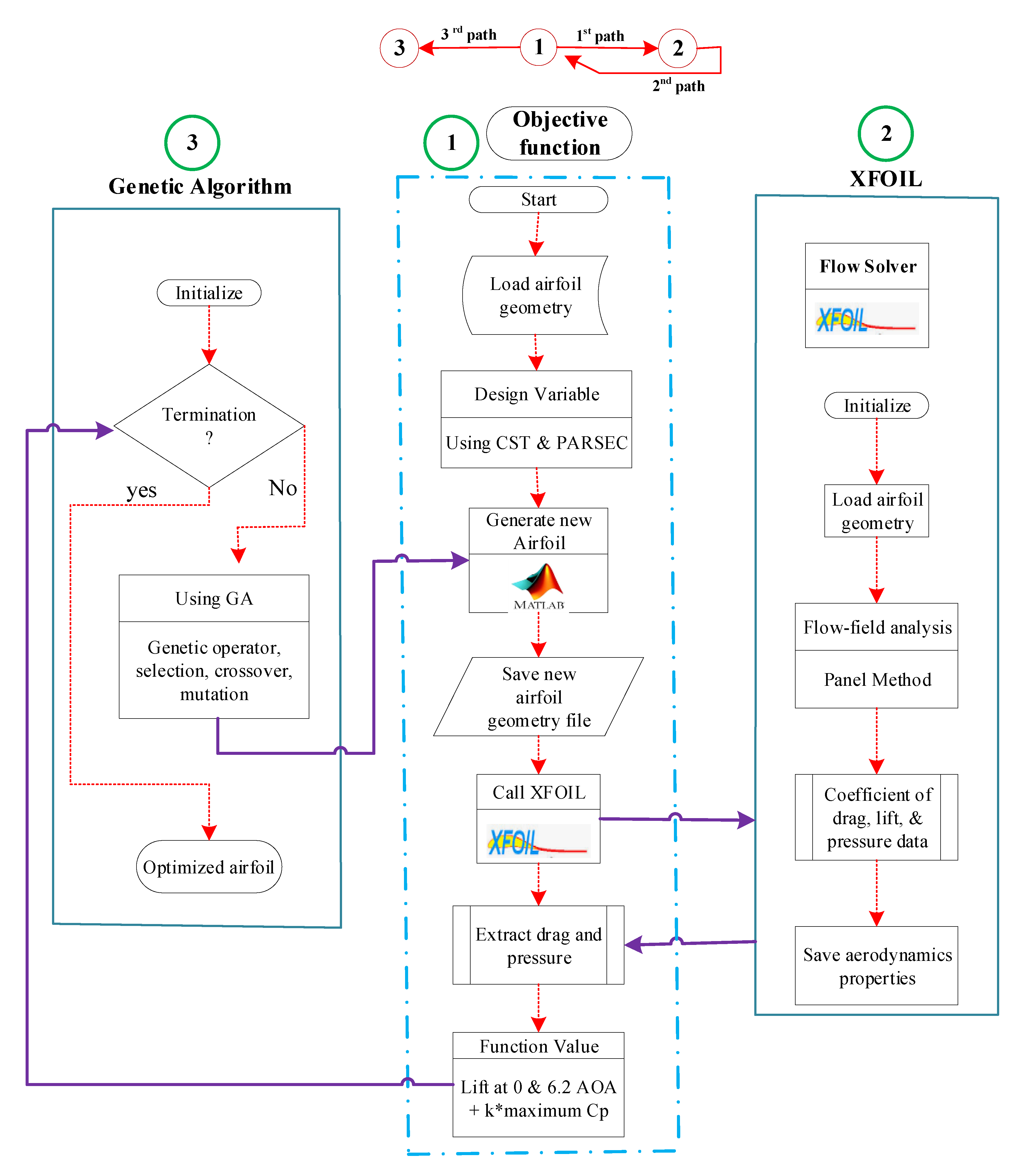
Airfoil shape optimization is a critical problem, due to the parameterization of the airfoil shape, CFD analysis of the flow field, and selection of the best and most suitable optimization algorithm. The parameterization technique uses shape change functions to represent a shape with fewer parameters without using a large number of coordinate points. This makes it significantly easier to handle the shapes with a few design variables. The code for airfoil shape optimization was developed using the MATLAB software. The methodology applied for aerodynamic shape optimization is shown below as a flow chart in Figure 5. The initial population consisted of the control variables of the test airfoil shape. With the help of the airfoil parameterization code, an input text file was created that contained the coordinates of the airfoil for flow field analysis. The XFOIL code in MATLAB was used for the aerodynamic analysis and for the aerodynamic properties, including lift, drag, and pressure coefficients, which were saved for the evaluation of the fitness function in the optimization algorithm. If the fitness criteria were achieved, the optimized airfoil shape coordinates were saved; otherwise, a new population set was generated to go through the same procedure. The airfoil parameterization method and the optimization scheme used for the present study are described in detail in the following subsections.
2.1. CST Parametrization
The class shape transformation (CST) method is a relatively powerful and effective parameterization technique that uses a Bernstein polynomial for modeling both two-dimensional and three-dimensional aerodynamic shapes. The CST method is not limited to airfoil shapes only, but it can also generate different aerodynamic shapes. The coefficients of two arrays, shown in Equations (1) and (2), were built to define the CST method and differentiate one airfoil from another. These CST array coefficients were controlled by the curvature of the lower and upper surfaces of the airfoil [12], while the curvature of the airfoil provided a set of design data that was further utilized in the main task of shape optimization [27]. This parameterization scheme covered a wide range of airfoils and made it equally applicable to any shape of the airfoil. As described later mathematically, CST consists of two main elements: a shape function and a class function. The class function of an airfoil deals with fixed parameters inside the class function itself. The smoothness of the curve plays an important role for the CST and Bernstein polynomial, which is beneficial for optimization purposes. The relation for the CST is stated in the next paragraph.
The relation for the upper and lower surface of the CST airfoil is shown below in Equations (1) and (2), and where C and S are the class and shape functions, respectively.
The upper and lower surfaces are defined by the following equations:
where and are the trailing edge thicknesses of the upper and lower surfaces, respectively. and , and both values remain constant.
The class function describes the main profile of the aerodynamic shape while the shape function creates a fixed shape within the same geometry class. The relation of the class function is shown in Equation (3):
All the airfoils which were represented by the CST method of parameterization were extracted from the class function. The exponents and , which define the type of geometry, are replaced by the values 0.5 and 1.0, respectively, to represent the upper and lower surfaces of the airfoil. To represent an airfoil, Equations (1) and (2) can be explained by
The general shape functions (for the upper surface) and (for the lower surface) define particular shapes within the same airfoil class. Equations (6) and (7) show the overall shape function:
where and are the upper and lower surface weights, respectively, and are the upper and lower surfaces for the CST order of the Bernstein polynomial, and S denotes the component shape function, which differs for the upper and lower surfaces on the basis of the order of the Bernstein polynomial.
The component shape function is written as
where is the binomial coefficient, and it is related to the order of the Bernstein polynomial. It is represented as
Equations (3)–(9) are combined to form complete equations of the upper and lower surfaces of airfoils and relations, as shown in Equations (10) and (11):
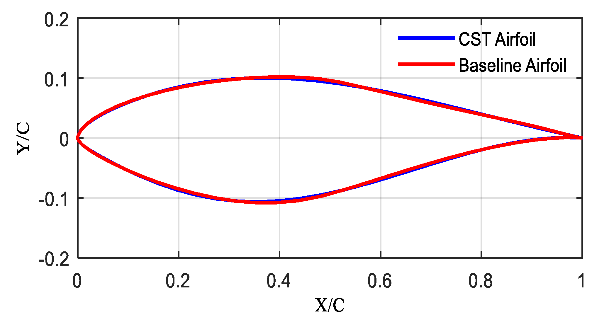
Equations (10) and (11) describe an airfoil that provides perfect curvature coefficients. These curvature coefficients are optimized to show a known airfoil profile. When the parametrization of an airfoil is performed by the CST method, a set of design variables is obtained which is utilized as the main task in the optimization process. Figure 1 shows the airfoil shape generated by CST parameterization using a second-order Bernstein polynomial, where N1 = 0.5 and N2 = 1.0. In the baseline of Figure 1, the red line represents the initial airfoil, and the blue dotted line represents airfoil generated by CST parametrization.
2.2. PARSEC Parametrization
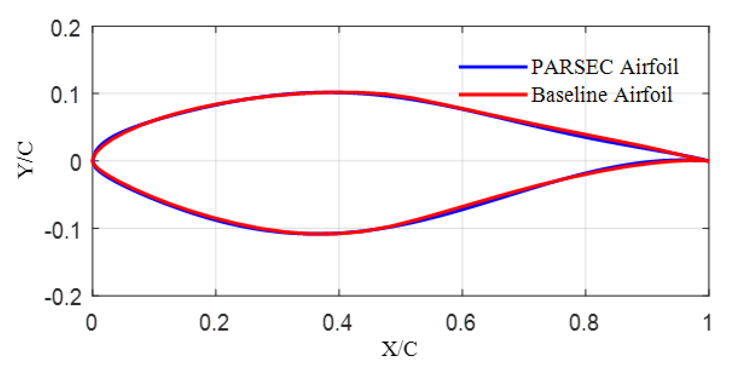
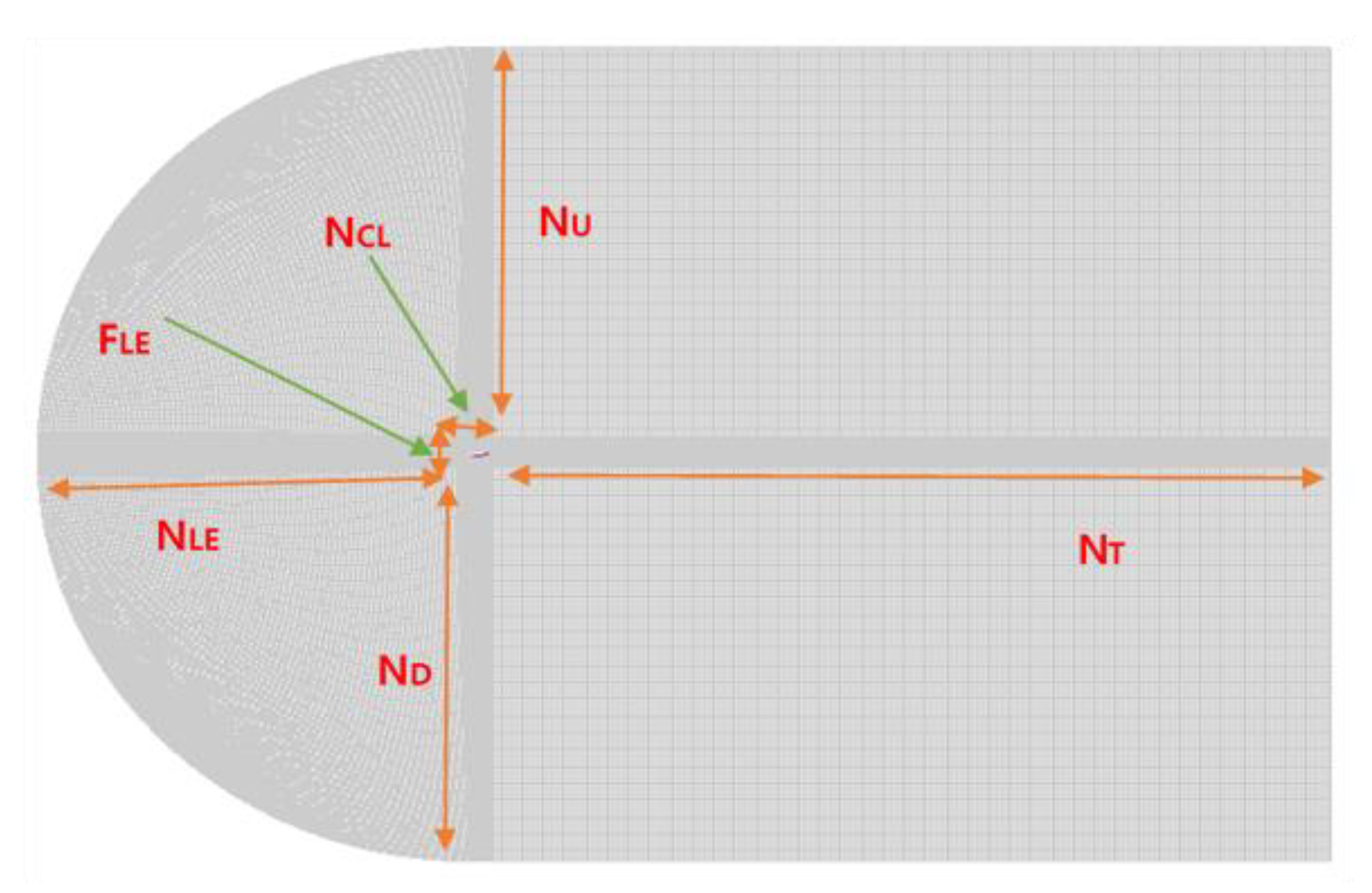
In the previous literature for the representation of different types of airfoils, the parameterization method was used to transform the shape of the airfoil with a minimum number of control points for aerodynamic optimization purposes. Sobieczky [21] developed a parameterization scheme called parametric section (PARSEC), which represents the shape of an airfoil using an unknown linear combination of the base functions. In the present study, the NREL S-809 was selected as the reference airfoil for parameterization and optimization purposes due to its high lift-to-drag ratio and better aerodynamic performance in comparison with low-camber and high-thickness airfoils, as established in the literature [28]. The NREL S-809 airfoil is achieved by solving a set of linear equations using twelve different airfoil geometry parameters. The PARSEC method uses these twelve geometric parameters because of the design variables that control the configuration of the airfoil. All twelve airfoil design parameters in geometrical and tabular form are demonstrated in Figure 2 and Table 1, respectively. Figure 3 compares the baseline airfoil with the airfoil generated by the PARSEC method. The NREL S-809 airfoil is divided into two parts,—the upper and lower sections—and both the upper and lower sections are represented by the sixth-order polynomials listed in Equations (12) and (13), respectively:
where and signify the y-coordinates of the upper and lower sections, respectively, is the normalized chord-wise coordinate, and and are the unknown coefficients for the upper and lower sections, to be determined by using the airfoil design parameters as follows:
where
2.3. Optimization Scheme
To achieve an optimal solution, numerical design techniques can help to solve challenging engineering problems. The proper selection of search algorithms for aerodynamic shape optimization is important because of the availability of variable fidelity optimization algorithms in the literature.
Based on the natural selection process, a genetic algorithm (GA) is an evolutionary algorithm in contrast to gradient optimization techniques. The GA was introduced by John Holland [29] in 1960 based on Darwin’s theory of evolution, and in 1989, it was extended by David E. Goldberg [30]. The solution for the optimization or search problem is obtained by estimating the fitness function for the initial population. A population consists of individuals or phenotypes that represent each candidate’s solution. Each candidate of the population has a set of chromosomes or a genotype. The initial population goes through the process of fitness testing, and a fitness score is assigned to each individual population. Performance evolution in the genetic algorithm is done by using bio-inspired processes (e.g., crossover, mutation, and selection). Fitness scores for individuals are selected on the basis of the highest fitness score for the offspring (new population pool). For the selection of new individuals or parents, the offspring or new population again undergoes the fitness evaluation. A genetic algorithm has the ability to provide solutions to complex discontinuous and multimodal design spaces, and it is widely used in non-gradient global search methods. Additionally, the genetic algorithm relies on gradient information as it uses a population of high fitness value design candidates to avoid locally optimal solutions. A genetic algorithm has the ability to carry out a global search, making it most suitable for aerodynamic shape optimization problems. Therefore, in this study, a GA is incorporated with the parameterization method to optimize the airfoil, using fewer control variables for the small wind turbine system.
The airfoil shape is represented by each chromosome (candidate solution), which contains a set of genes (design variables) within a population (search pool). The solution for each candidate’s fitness score depends on the lift coefficient of the airfoil, as the purpose of the objective function is to maximize the airfoil lift coefficient. The characteristics of the genetic algorithm are very important and play an important role in determining the accuracy and computational cost of the algorithm. The characteristics of the genetic algorithm have been selected in correspondence with the guidelines provided by Williams and Crossley [31]. Therefore, it was decided to increase the population size to four times the string length for this investigation. The mutation rate is calculated using Equation (20) while the crossover rate is set to 0.5, which results in a decent fitness score with a good relative computation economy:
where , , and are the probability of mutation, string length, and population size, respectively. The objective behind this optimization scheme is to maximize the lift coefficient of the airfoil. Multiple termination criteria were imposed in the code for the convergence of the genetic algorithm (i.e., on the basis of the difference in the fitness maximums, consecutive maximum fitness values, and bit string affinity values). The single-objective function for optimization of an airfoil shape is written as follows:
The objective was to find the maximum aerodynamic efficiency value and the best airfoil representation by maximizing the lift coefficient () and lift-to-drag (L/D) ratio. The GA was employed for aerodynamic design optimization in a large design space. The geometric limitations, aerodynamic constraints, and optimization criteria used for airfoil optimization have been listed in Table 2. Below, Figure 4 shows the optimized airfoil shape profile of the baseline airfoil (NREL S-809).
3. Methodology
The whole transformation and optimized airfoil were generated using an integrated aerodynamic shape optimization MATLAB code for airfoil parametrization (i.e., CST and PARSEC aerodynamic performance evaluation and genetic algorithm-based optimization). For this study, a well-known existing airfoil, the NREL S-809, was selected instead of designing a new airfoil with the common application. The NREL S-809 airfoil generates a high lift-to-drag ratio at a stall angle, which is beneficial for the blade design of a small wind turbine. In this study, aerodynamic shape parameterization by the PARSEC and CST methods was employed for the airfoils in the MATLAB environment. These parameterization methods were further linked with a genetic algorithm in the in-house MATLAB code for optimization purposes. XFOIL was used for the evaluation of the flow field analysis, which used the panel technique to calculate the coefficient of lift, drag, and pressure data for optimized airfoil geometries for angles of attack from 0° to 6.2°. On the other hand, for the NREL S-809 airfoil, a CFD computational study on the ANSYS CFX using structured mesh was performed for both the baseline and optimized airfoil obtained after the parameterization and optimized process from the MATLAB-based method at a 6.2° AOA. The overall methodology is organized in a flowchart as shown in Figure 5.
3.1. Computational Model
The Reynolds-averaged Navier–Stokes (RANS) and continuity equations are used to compute the compressible flow field in the steady state. The equation for mass and the momentum conservation equations in each direction with no source term can be written as shown in Equations (22) and (23). In addition, to solve the Reynolds stress term, a shear stress transport (SST) turbulence model is used, due to its ability to accurately predict aerodynamic features such as the flow boundary layer, pressure drop, flow separation, and recirculation:
where is the density, is the pressure, is the dynamic viscosity, and is the body forces, while and are called the velocity vectors for the related values of . Due to the unknown Reynolds stress term, the RANS turbulence model equation must be closed, but the RANS equation is not closed [32]. For the better prediction of aerodynamic data, pressure drop flow recirculation, precise boundary layer calculation, and flow separation are essential. Some people use the wall function of the flow model within the boundary layer in the RANS turbulence model, but this type of turbulent model is not suitable to provide an accurate prediction of the boundary layer, flow maintenance, pressure drop, and flow separation. Direct numerical simulations (DNS), large eddy simulations (LESs), and detached eddy simulations (DESs) [33,34] are some very expensive computational techniques; therefore, the SST turbulence model was adopted for the numerical study to achieve aerodynamic data with precise prediction, along with the advantages of the computational economy [27]. The shear stress transport turbulence model is an amalgam of the Wilcox and turbulence models. The turbulence model is used to solve the flow in a fully turbulent region to benefit from its economy, robustness, and free stream independence, while the Wilcox turbulence model is employed to solve the flow near the walls for precise prediction of the boundary layer [35]. The two equations of the SST turbulence model for the turbulent kinetic energy () and the turbulent dissipation rate () are given as follows in Equations (24) and (25), respectively:
where is the blending function defined in Equation (26). The value of is zero away from the wall and allows the model, while the value being near 1 within the boundary layer enables model:
is a cross-diffusion term in Equation (27), and it is expressed as
The terms on the left side of Equation (25) represent the rate of change of and transport of , while for Equation (26), the left side of the equation represents the rate of change of and transport of . On the other hand, for Equations (25) and (26), the terms at the right-hand side represent the rate of production, turbulent diffusion, and rate of diffusion of and , respectively.
The effective velocities and are defined in Equations (24) and (25) as follows:
where is the turbulent viscosity, given as follows in Equation (30):
where is a second blending factor, given as follows:
Furthermore, the details and values of the constants for the SST turbulence model can be found in [35].
3.2. Computational Model
In this paper, aerodynamic shape optimization of an NREL S-809 airfoil has been presented by using a genetic algorithm for the NREL Phase II, Phase III, and Phase VI HAWT blade designs. These blades were composed of an NREL S809 airfoil from root to tip. Therefore, for better performance, the blade design of the S809 airfoil was optimized using different boundary conditions. For the numerical simulation, a 0.75 million Reynolds number was considered and compared with the experimental data of the original airfoil provided by The Ohio State University (OSU) in order to validate the present simulation [23]. The Reynolds number and Mach number were considered in the range of incompressible flow at angles of attack of 0° and 6.2°. The initial inputs and boundary conditions for the simulation are shown in Table 3.
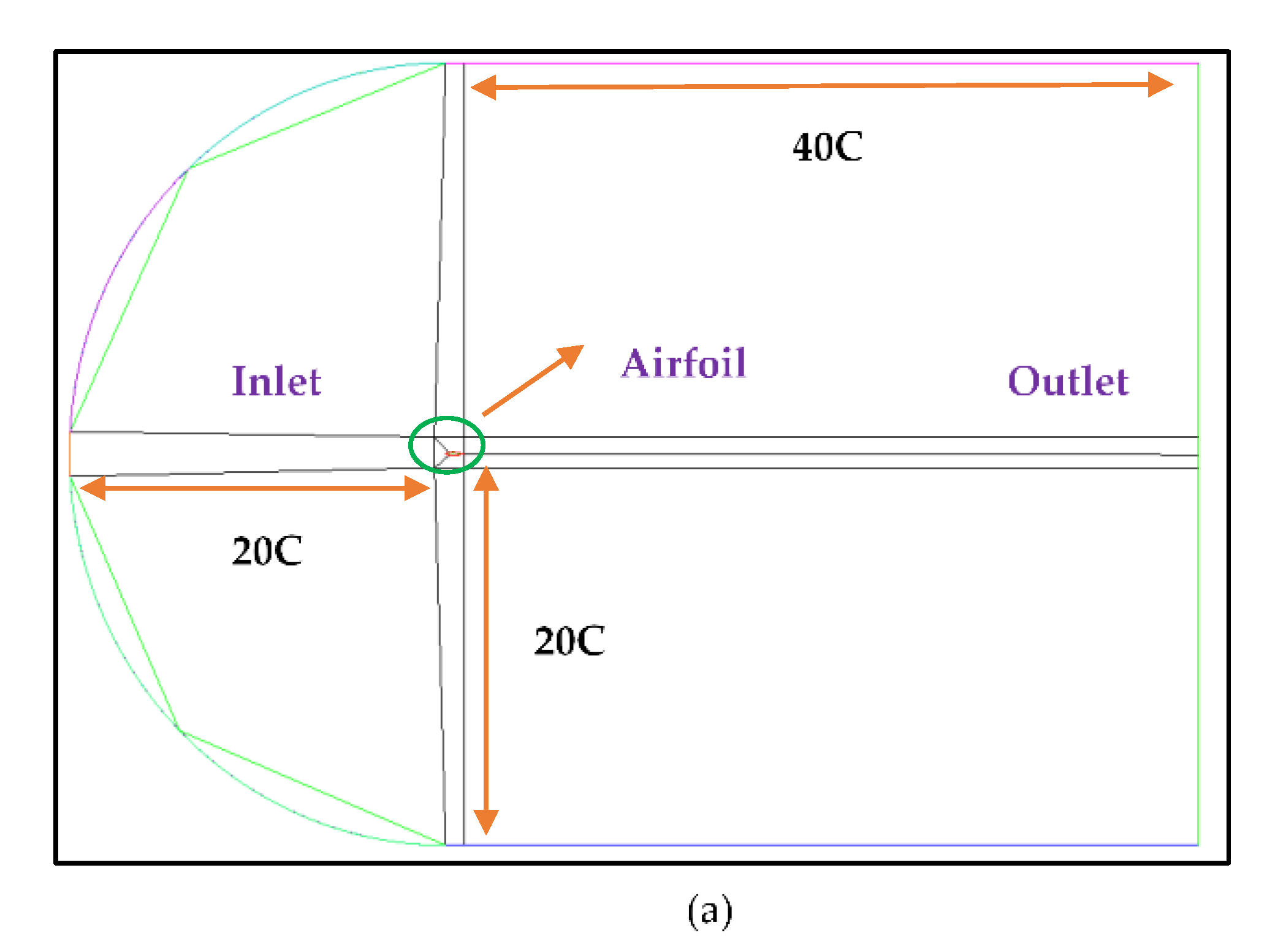
3.3. Mesh Generation
To eliminate the effect of the domain, the flow domains of the airfoil were subdivided into smaller subdomains to analyze the fluid flow. The computational domain was discretized into nodes by ANSYS-ICEM CFD, and the governing equation was used to solve each and every node. To ensure that the interface boundaries had a 1:1 node connection, a meshing topology was adopted for both domains to avoid interpolation losses in the interface. The O-grid topology was employed to generate a structured grid for the overall computational domain. This type of blocking ensures reduced computational cost and interpolation losses. In addition to this, the fine mesh was maintained to achieve a turbulence model dependent (<1 for the SST turbulence model) [36]. Figure 6 and Figure 7 depict the details of the mesh topology and the grid generation around the computational domain. The main purpose for adopting the O-grid topology was to have better and more uniform control of the near-wall mesh. The value should be always maintained at a value less than 1 within the domain of the airfoil to get the benefit of the SST turbulence model [13]. The value is a function of (first node’s distance from the wall), Re, and the flow length (L). The relation given in Equation (32) was used to calculate the value of and to get the value [28]. The equation to calculate was derived for the flow over the flat plate; therefore, it only provided initial estimates of for the airfoil geometries. To get a value, no more than a few iterations were required to finalize the value of for a specific set of boundary conditions:
Besides having a certain value of , some different values for the minimum number of nodes () within the boundary layer thickness () were also required. For the SST turbulence model, the condition for () is stated in Equation (33):
where (15) is the distance of the fifteenth node. The relation given in Equation (34) was used to calculate the value of the boundary layer thickness at a specific value of and :
The value of the boundary layer thickness calculated in Equation (34) was assigned to , and the mesh growth rate () from the wall side was computed by the relations of geometric progression shown in Equations (35) and (36) within the boundary layer thickness:
3.4. Grid Independence Study
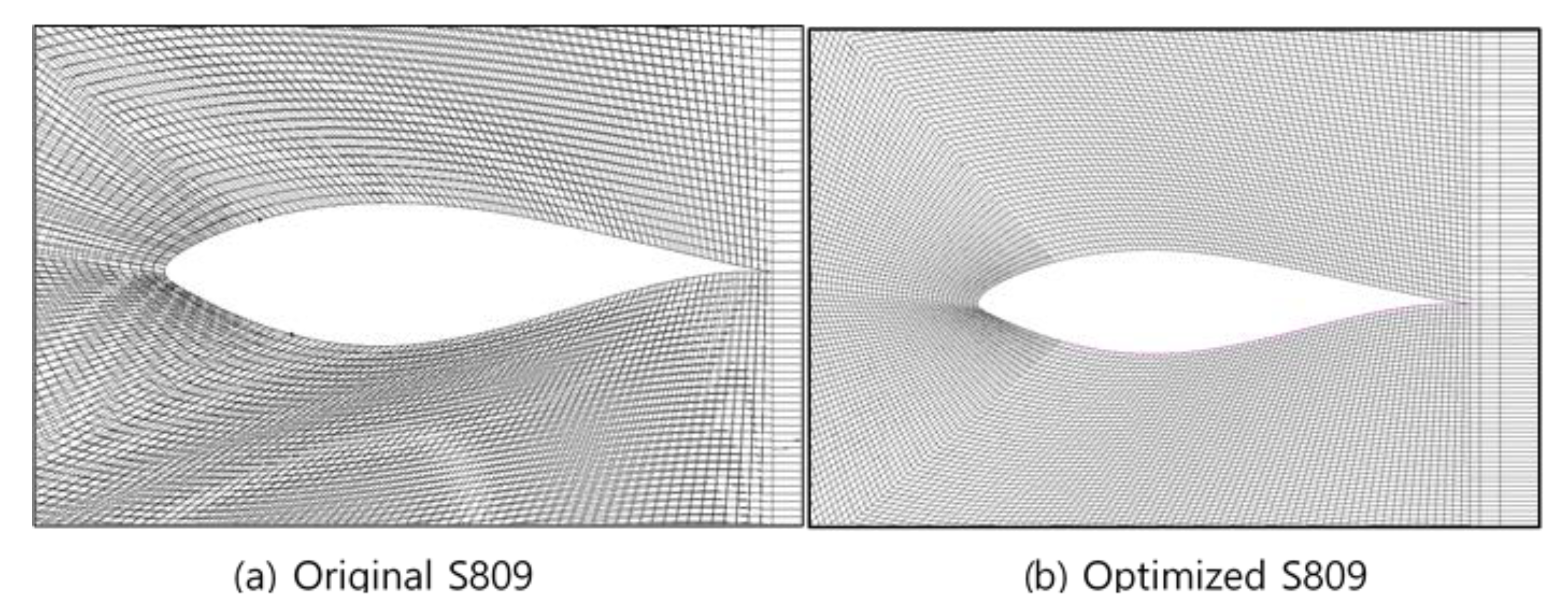
In order to get the mesh independent solution, a grid sensitivity analysis was conducted using four different meshes—M1, M2, M3, and M4—by varying the grid resolution from 3.6 million to 8 million. The details of the mesh independence study are described in Table 4. The nodes along the upward direction (), nodes along the downward direction ), and nodes along the airfoil length () were kept constant and equal in number for all four mesh independent studies. The nodes along the trailing edge () and leading-edge () were increased by a count of 50, whereas the nodes along the radial direction () and in front of the leading edge were increased by a count of 25 from the initial counts. Hence, every time mesh was loaded and generated to run the simulation on ANSYS 16 [36]. The steady-state simulation for all four meshes (M1–M4) was carried out with a wind speed of 7 m/s. After each mesh independence study, the , , allocated memory, and CPU times for 10 iterations were recorded by the solver and compared with the other one. On the basis of and , the transition from M3 to M4 resulted in an error recovery of less than 1%. Therefore, by considering the grid resolution and computational accuracy, M3 was selected to perform all the subsequent simulations in the present study. The distribution of the mesh topology with a specific name in the computational domain for the mesh independence study is shown below in Figure 8. The mesh distribution in the computational domain is listed in Table 4 with other details.
4. Results and Discussion
This section presents the optimization results obtained from the coupling of the CST and PARSEC parameterization methods with the genetic algorithm (GA) optimization process for the well-known existing NREL S809 airfoil for the design of the NREL Phase II, Phase III, and Phase VI HAWT blades of the wind turbine. The optimization results of the S809 airfoil are further compared with the experimental data from The Ohio State University (OSU) [26]. Furthermore, upon comparing the optimization results between CST and PARSEC, the best option with a higher lift-to-drag ratio was selected for the CFD simulation for validation purposes. The main objective behind the aerodynamic shape optimization and CFD simulation of an airfoil was to maximize the coefficient of lift () and the lift-to-drag (L/D) ratio. The whole optimization process was carried out through coding in MATLAB, and XFOIL was used to calculate the , , and pressure data. XFOIL uses the panel technique method for the calculation of pressure data and the coefficient of pressure (Cp). For the CFD simulation of the airfoil, ANSYS ICEM was used as meshing software, while ANSYS CFX was considered for discretizing the governing equation and running the simulation. A framework and blocking were created around the airfoil for the meshing to capture the boundary wall of the airfoil and solve the governing equation on each and every node at a given set of conditions, shown in Table 3. A total of eight design variables were used for the CST method to design an S809 airfoil with a polynomial order of three degrees, while the PARSEC parameterization method used twelve basic parameters to generate a new airfoil design. The main role of this design parameter was to calculate the proper upper and lower bounds of the airfoil within the specified range of 20%. The design parameters are depicted below in Table 5.
4.1. Verification and Validation
In this section, the results from the studies performed on airfoil optimization are discussed and presented. First, the ability of the CST method employed with a genetic algorithm to produce an optimized S809 airfoil was tested. Secondly, the PARSEC method was coupled with the GA to generate an optimized airfoil from the existing baseline S809 airfoil. The flow field conditions used by the optimization process to investigate the , and lift-to-drag (L/D) ratio were Re = 0.75 million, AOA = 0° and 6.2°, Mach number (Ma) = 0.02, and a wind velocity of 7 m/s. To normalize the chord length (c) for the airfoil, it was set to 0.34 m. During the optimization process, the CST and PARSEC variable parameters played an important role in describing the airfoil shape. Further airfoil shaping was defined by the upper and lower curvatures of the airfoil, which provided a design set of data. For every design variable, the lower and upper bound values were defined in the GA optimization code in MATLAB. As a result, the GA produced the best sets of CST and PARSEC parameters and, hence, an optimized airfoil profile was generated. These optimized airfoils were tested at a given set of conditions for the calculation of the , , and pressure distribution curve with the in-house MATLAB program XFOIL. The new , , and L/D ratio obtained after the optimization process were compared with the original airfoil, based on the NREL experimental data provided by OSU [37]. The performances of the initial and optimized airfoils are compared and displayed in Table 6. As a result, it can be seen that the optimized result of the CST method was better than the NREL-based experimental data of the original NREL S-809 airfoil.
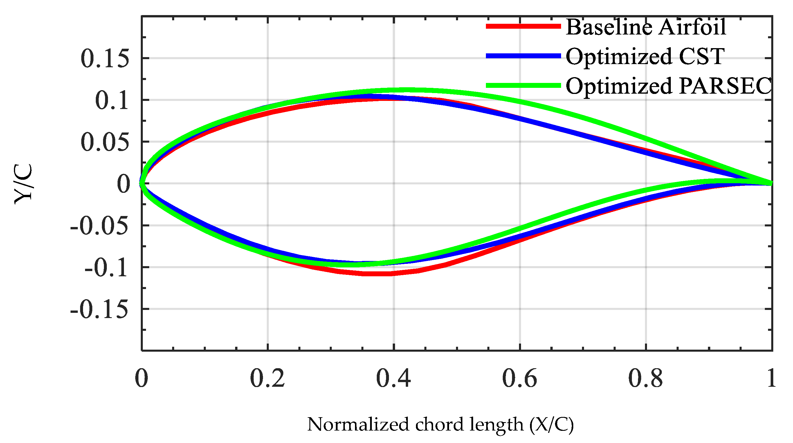
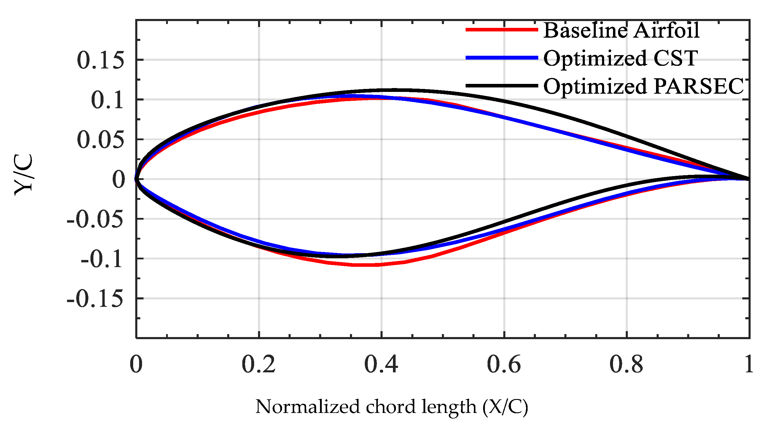
From Table 6, it can be seen that the was maximized and the L/D ratio was better for the S809 airfoil optimized by the CST method in comparison with both the baseline airfoil and the airfoil optimized by the PARSEC method. While comparing the CST and PARSEC methods with the experimental results of the S809 airfoil, it can be observed that the optimized airfoils for CST and PARSEC showed improvements of 11.8% and 10.1%, respectively, in the coefficient of lift (). However, this increment in the led to an improvement in the L/D ratio by 9.6% for the CST method, while the PARSEC method showed a decrease in the L/D ratio by 2% compared with the experimental results. From this, it can be concluded that optimization by CST gives better performance than another parameterization method. Figure 9 displays the optimized S809 airfoil profile generated by the CST and PARSEC methods and the baseline airfoil.
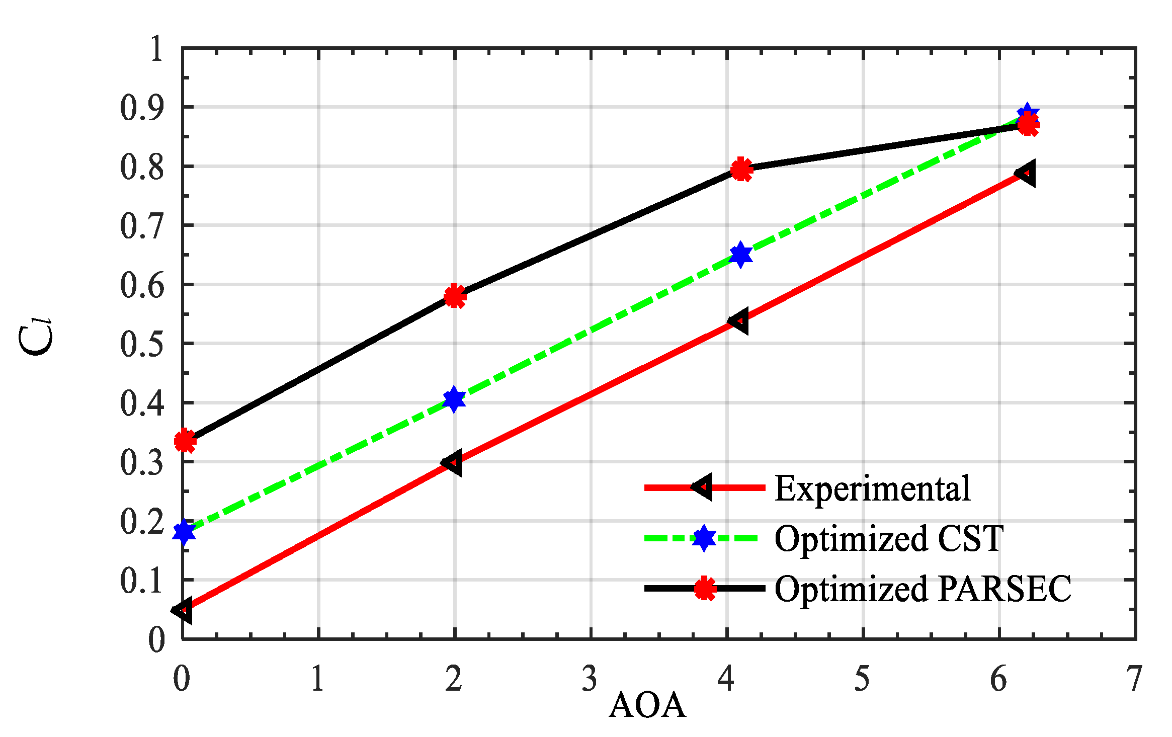
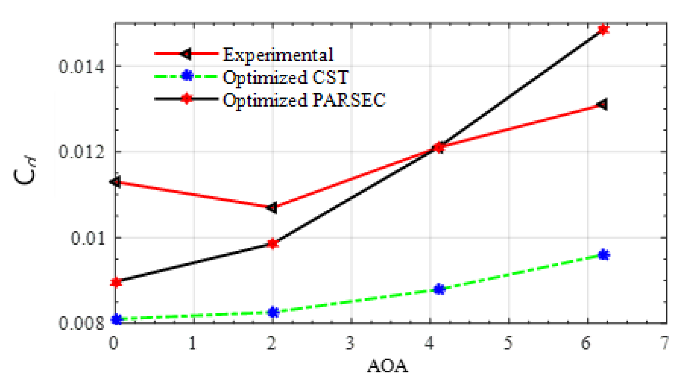
Figure 10 demonstrates the variation of lift coefficient with the increase in the angle of attack. It is observed that increased in all three profiles as the angle of attack increased from 0° to 6.2°. By looking at the figure, it can be concluded that the optimized CST airfoil gave a better performance than the experimental and PARSEC methods. For the blade design, was kept at a high level, which implied a good off-design property of the small wind turbine. Figure 11 shows the coefficient of drag, which was a very difficult quantity to calculate numerically as well as experimentally. By the CST methodology, the drag was minimized the most compared with the other drag coefficients calculated experimentally by OSU and by the PARSEC method. For the lift coefficient and L/D ratio, the present results gave a slightly higher value than the experimental results provided by OSU [37]. The comparisons and calculations used in this paper validate our numerical methodology.
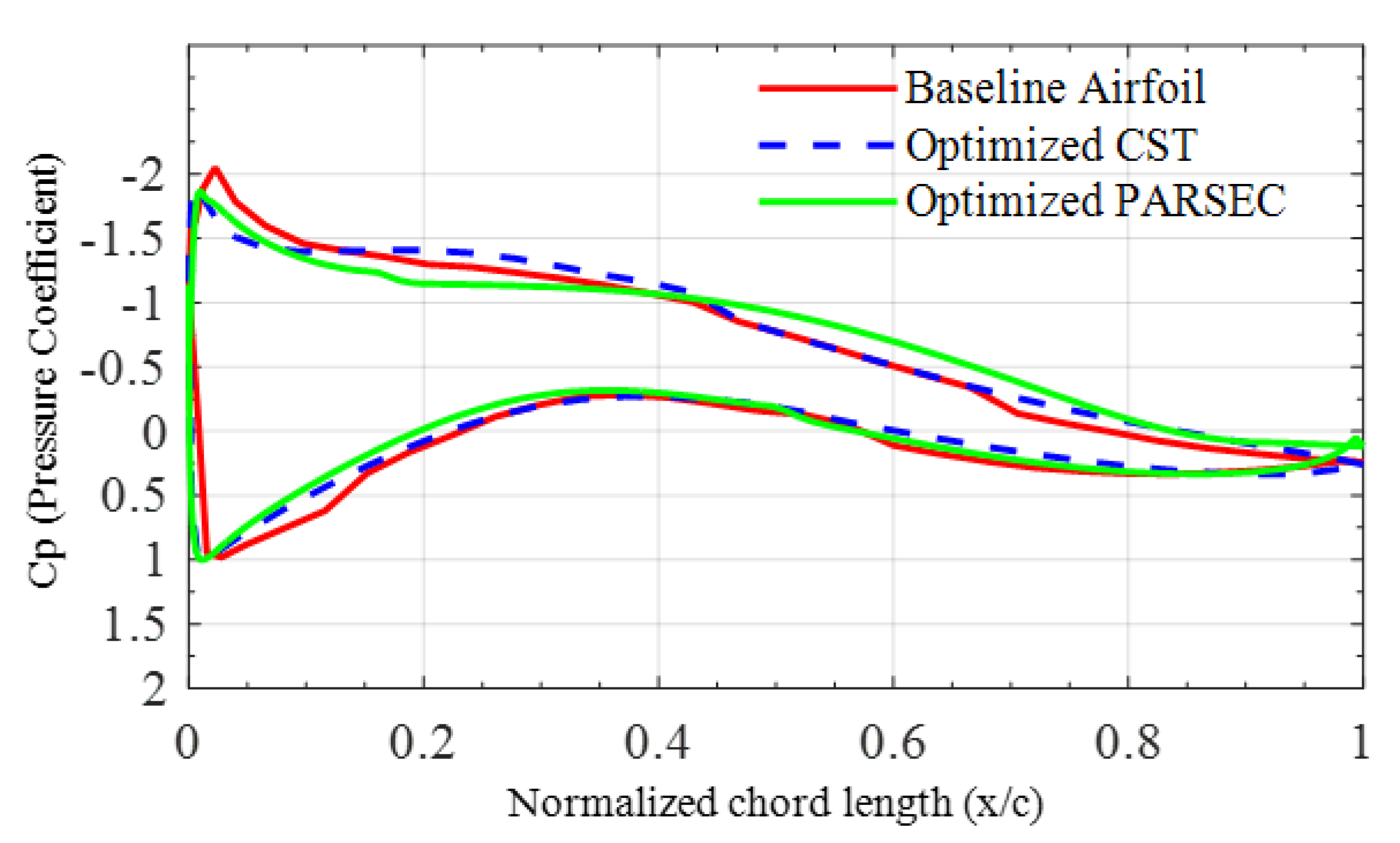
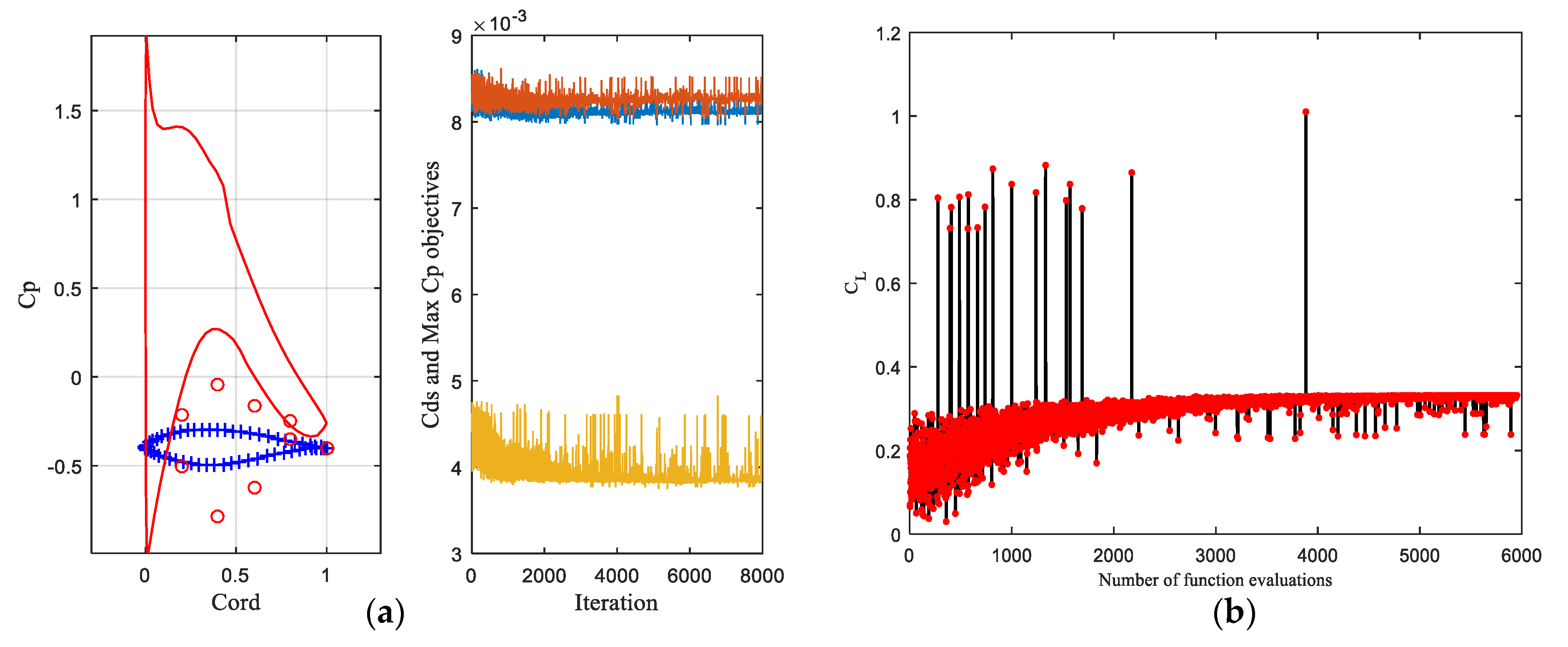
The pressure distribution over the surface of the baseline airfoil and the optimized airfoil obtained by the CST and PARSEC methods at a 6.2° angle of attack were compared by drawing a pressure coefficient (Cp) graph, shown in Figure 12. It was found that the Cp values obtained from XFOIL simulation were relatively high for both the optimized airfoil and the baseline airfoil. XFOIL uses a panel technique method to calculate the pressure distribution over the upper and lower surfaces of the airfoil. These are the aerodynamic properties of an airfoil which are the direct result obtained from the design objective. Figure 13 shows the convergence graph of an optimized airfoil for the CST and PARSEC parametric methods with 8 and 12 basic design parameters, respectively. Figure 13a displays error bars with respect to the number of iterations and the pressure distribution curve at a 6.2° angle of attack, while Figure 13b shows the iterations of function evaluations used to converge the airfoil with the lift coefficient. The residual pressure at the surface of the optimized airfoil generated by CST was very small, and the geometry residuals were below 3 × 10⁻³. The time consumed by the algorithm of the CST and PARSEC optimization processes was 210 and 272 min, respectively. This shows that CST, with fewer parameters, consumed less time than PARSEC with 11 basic parameters. Moreover, a comparison of the optimization results between CST (n = 6) and CST (n = 8) was also performed. It was concluded that the optimized results were obviously better than those of the baseline airfoil, but the CST parametric method with eight design parameters was better than that with six parametric variables. As a result, eight design variables were used for optimization purposes, and the airfoil shape that corresponded to the optimal objective values was the final shape of the optimized airfoil.
4.2. Numerical Validation
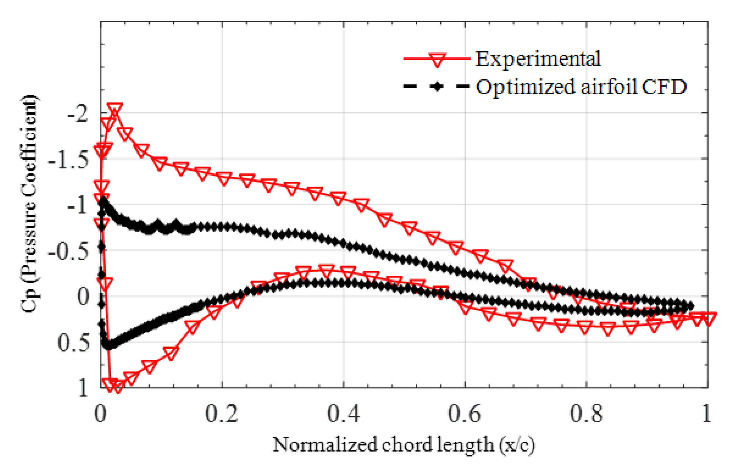
After the comparison of the lift-to-drag ratio (L/D) for the optimized S809 airfoil generated by the coupling of the CST and PARSEC parameterization methods with a genetic algorithm generated by XFOIL, the optimized S809 airfoil originated by the CST and GA gave a significantly better lift-to-drag ratio in comparison with the PARSEC method. Therefore, the optimized NREL S809 airfoil originating from the CST method was simulated at different flow conditions, using CFD for validation of the results with the experimental data provided by The Ohio State University (OSU) [26]. An individual comparison based on (CST and GA) optimized geometry was validated in the CFD–CFX environment. TheS809 airfoil generated by the coupling of CST parametrization and GA optimization was further validated numerically. The simulation was run for the optimized S809 airfoil at angles of attack of 0° and 6.2° and at the same boundary conditions shown in Table 3 in order to compare the results with the existing experimental data from the reliable, NREL-based data source provided by OSU. Some of the forces applied to the airfoil were usually resolved into two forces and one moment. For the total components, the net forces acting normal with the incoming flow stream are known as the lift forces, and the net forces acting parallel to the incoming flow stream are known as the drag forces. Table 7 shows the lift and drag coefficients of the baseline and optimized airfoils and their computational fluid dynamics simulation data. The L/D ratio for the optimized airfoil was approximately 12.4% higher than that of the experimental data of the baseline S809 airfoil. It is also clearly shown that the computed by the turbulence model for an optimized airfoil at a 6.2° angle of attack was 12.2% better than the experimental results of the original airfoil. Figure 14 shows the pressure distribution (Cp) over the upper and lower surfaces of the baseline and the optimized airfoil calculated by CFD analysis. It can be observed from the Cp graph that the pressure calculated by CFD had a lower negative pressure on the lower surface of the optimized airfoil. As a result, lift generation was greater in the optimized airfoil compared with the baseline, and this implied better aerodynamic properties for the blade design of the wind turbine.
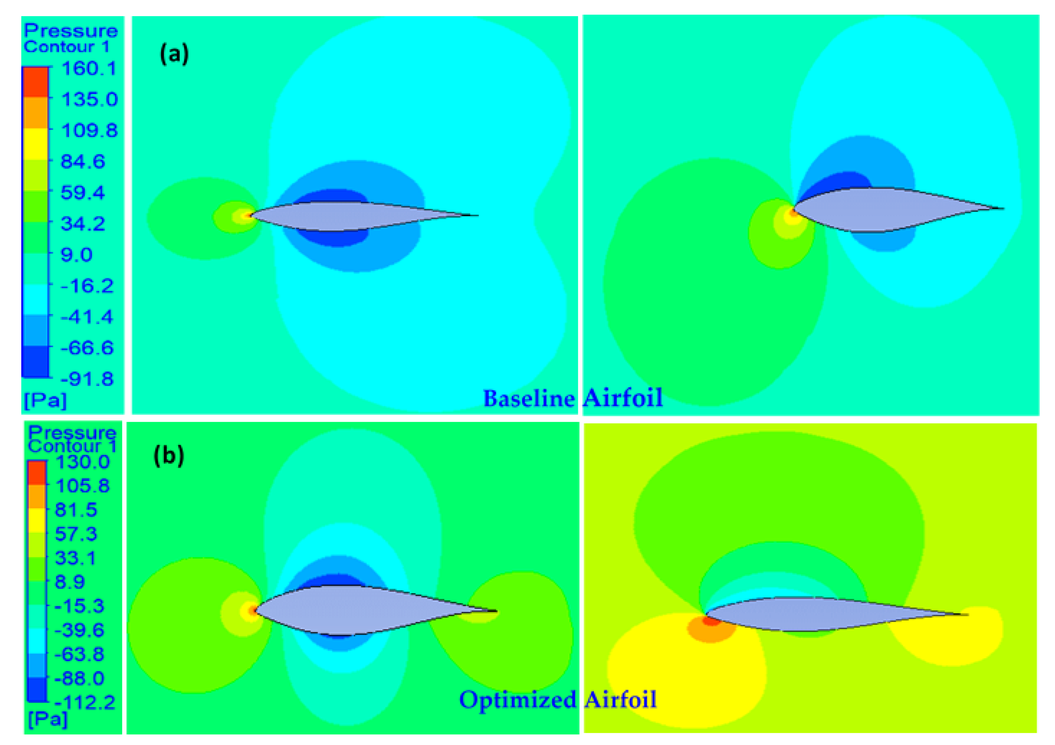
Figure 15 shows the simulation outcomes of the static pressure over the upper and lower surfaces of the baseline and optimized S809 airfoils in a wind speed of 7 m/s at angles of attack of 0° and 6.2°. The baseline and optimized airfoils with pressure contours are shown in Figure 15a,b, respectively. The left side of the figure displays the pressure contour at 0°, while the right side shows the pressure contour at a 6.2° angle of attack. Figure 15 clearly depicts that more negative pressure was observed over the upper surface of the baseline airfoil than the optimized airfoil, and hence more lift was generated in the optimized S809 airfoil. Consequently, the airfoil was pushed upward effectively, normal to the incoming flow stream. As a result, the S809 airfoil produced better aerodynamic properties for the design of the blade of the wind turbine.
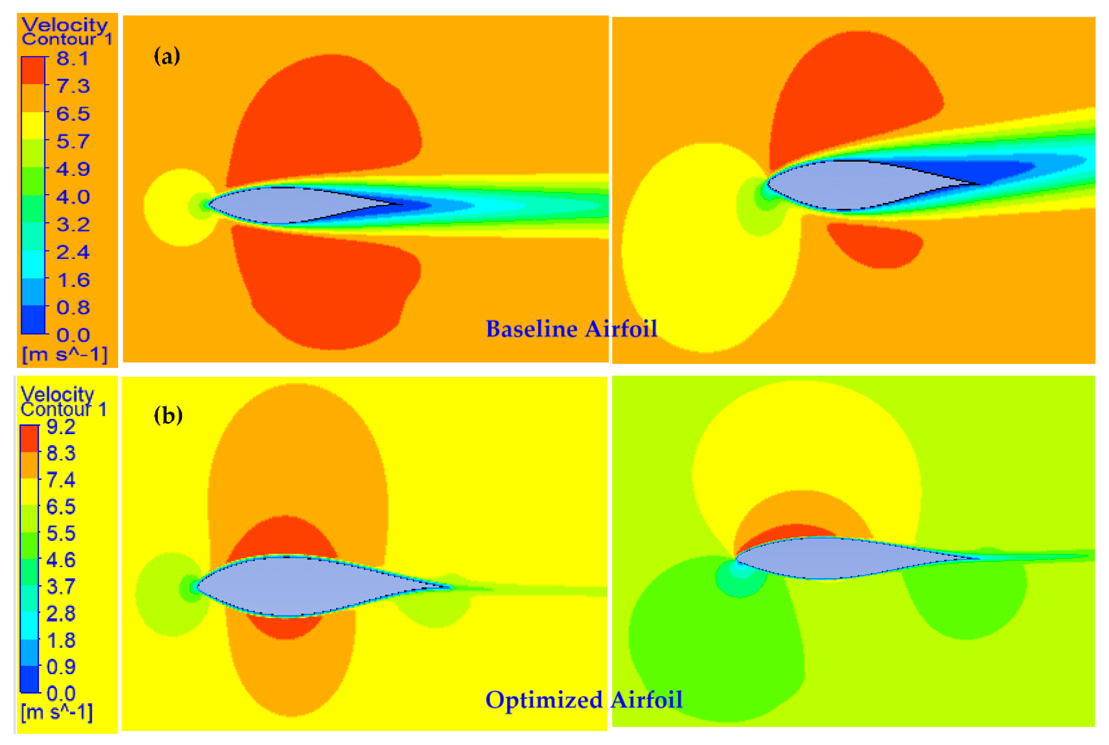
The velocity contours shown in Figure 16 are consistent with the results at angles of attack of 0° and 6.2°. The baseline and optimized airfoils with velocity contours are shown in Figure 16a,b, respectively. The left side of the figure shows the velocity contour at an angle of attack of 0°, while the right side shows the velocity contour at 6.2°. The lower surface of both the baseline and optimized airfoils experienced a slightly lower velocity compared with the upper surface of the airfoil. The stagnation point of the airfoil changed by changing the AOA, and it mostly lied near the leading in the lower surface of the airfoil. An increase in the angle of attack increased the upper surface velocity to a point much higher than that of the lower surface velocity. For the CFD simulation and optimization, we considered 7 m/s wind speeds to calculate the other aerodynamic properties of the airfoil, (e.g., coefficient of lift (), coefficient of drag (), and lift-to-drag (L/D) ratio) for the blade design of wind turbines.
Based on the above discussion, it can be concluded that simplified CST parametrization with a genetic algorithm resulted in the optimized airfoil shape formation for the NREL S809 airfoil, which behaved as a general trend for airfoils but with better flow characteristics and aerodynamic performance. This provides further confidence in utilizing this methodology for different shapes of airfoils for the blade designs of different wind turbines. Nevertheless, the novelty of the investigated approach can be marginally justified as a readily applied technique in the energy sector by reassuring the expected results against the CFD-derived data.
5. Conclusions
In this paper, a genetic algorithm was coupled with the CST and PARSEC parameterization methods and employed to optimize the aerodynamic shape of a well-known wind turbine, the NREL S-809 airfoil, to improve its lift and drag characteristics in order to achieve its two objectives, those being to increase its lift and lift-to-drag ratio for a wind turbine. This has been presented and applied to find the optimal shape of the NREL Phase IV HAWT blades. The optimization scheme was carried out with MATLAB code, which utilized the XFOIL solver for an iterated process to calculate the lift, drag, and pressure data. At the final step, the commercially available ANSYS CFX software was used to simulate the flow field on a structured mesh using the Reynolds-averaged Navier–Stokes (RANS) equation in combination with the two-equation and SST turbulence model. However, the results showed significant improvement in the coefficient of lift and lift-to-drag ratio of the optimized airfoil compared with the original S809 airfoil. The following conclusions were derived:
- The airfoil optimized by CST showed an increment of 11.8% in the lift coefficient and 9.6% in the lift-to-drag ratio, while with PARSEC, it showed an improvement of 10% in the coefficient of lift and decrease of 2% in the overall lift-to-drag ratio while comparing both optimized NREL S809 airfoils;
- The proposed methodology, in terms of the lift-to-drag ratio, which is the vital decisive factor in blade and wind turbine design, exhibited superior aerodynamic characteristics by 11.6% in the optimization process with CST compared with the PARSEC methodology;
- The CFD analysis of the optimized airfoil showed an improvement of 24.6% in the lift coefficient and 12.4% in the lift-to-drag (L/D) ratio when comparing the optimized airfoil with the original S809 airfoil’s experimental results (OSU);
- The present aerodynamic optimization scheme was in close agreement with the previous results, and further application of the CST approach can be deployed with reasonable flexibility in other competitive optimization techniques;
- A significant reduction in the number of different design parameters offered a smaller number of genes for the candidate solution, which further enabled the search algorithm to act comparatively more efficiently and, in a time, -bound manner.
Author Contributions
Conceptualization, methodology, formal analysis, and original draft preparation by M.T.A., M.-H.K. supervised the research and edited the manuscript. All authors have read and agreed to the published version of the manuscript.
Funding
This research received no external funding.
Institutional Review Board Statement
Not applicable.
Informed Consent Statement
Not applicable.
Data Availability Statement
Data is contained within the article.
Conflicts of Interest
The authors declare no conflict of interest.
Nomenclature
| Aerodynamic shape optimization | |
| Class function | |
| Chord length (m) | |
| Drag coefficient | |
| Lift coefficient | |
| Pressure coefficient | |
| Class shape transformation | |
| Direct numerical optimization | |
| Direct numerical simulation | |
| Genetic algorithm | |
| Inverse design | |
| Binomial coefficient | |
| L/D | Lift-to-drag ratio |
| Ma | Mach number |
| Order of Bernstein polynomial | |
| n | Number of design variables |
| Function exponent of the first class | |
| Function exponent of the second class | |
| National Renewable Energy Laboratory | |
| Crossover probability | |
| Mutation probability | |
| PS | Population size |
| Reynolds-averaged Navier–Stokes equation | |
| Reynolds number | |
| Shape function | |
| Lower shape function | |
| Upper shape function | |
| Trailing edge thickness | |
| Greek Symbols | |
| Angle of attack | |
| Turbulence modeling constant | |
| Airfoil thickness | |
| density (kg/m3) | |
| Effective viscosity | |
| Turbulent viscosity | |
| Viscosity | |
| Boundary layer thickness | |
| Angular speed (rad/s) | |
References
- Twidell, J.; Weir, T. Renewable Energy Resources; Taylor & Francis: Oxfordshire, UK, 2005. [Google Scholar] [CrossRef]
- Ellabban, O.; Abu-rub, H.; Blaabjerg, F. Renewable energy resources: Current status, future prospects and their enabling technology. Renew. Sustain. Energy Rev. 2014, 39, 748–764. [Google Scholar] [CrossRef]
- Suman, S.; Kaleem, M.; Pathak, M. Performance enhancement of solar collectors—A review. Renew. Sustain. Energy Rev. 2015, 49, 192–210. [Google Scholar] [CrossRef] [Green Version]
- Taseska, V.; Markovska, N.; Callaway, J.M. Evaluation of climate change impacts on energy demand. Energy 2012, 48, 88–95. [Google Scholar] [CrossRef]
- Schaeffer, R.; Salem, A.; Frossard, A.; De Lucena, P.; Soares, B.; Cesar, M. Energy sector vulnerability to climate change: A review. Energy 2012, 38, 1–12. [Google Scholar] [CrossRef]
- European Commission. The Roadmap for Transforming the EU into a Competitive, Low-Carbon Economy by 2050; European Commission: Brussels, Belgium, 2011. [Google Scholar]
- United Nations Framework Convention on Climate Change; Paris Agreement: Paris, France, 2015.
- GWEC. Global Wind Report 2019; GWEC: Brussels, Belgium, 2019. [Google Scholar]
- Shahrokhi, A.; Jahangirian, A. Airfoil shape parameterization for optimum Navier–Stokes design with genetic algorithm. Aerosp. Sci. Technol. 2007, 11, 443–450. [Google Scholar] [CrossRef]
- Zhu, W.J.; Shen, W.Z.; Sørensen, J.N. Integrated airfoil and blade design method for large wind turbines. Renew. Energy 2014, 70, 172–183. [Google Scholar] [CrossRef] [Green Version]
- Song, W.; Keane, A. A Study of Shape Parameterisation Methods for Airfoil Optimisation. In Proceedings of the 10th AIAA/ISSMO Multidisciplinary Analysis and Optimization Conference, Albany, NY, USA, 30 August–1 September 2004; pp. 1–8. [Google Scholar]
- Orman, E.; Durmus, G. Comparison of shape optimization techniques coupled with genetic algorithm for a wind turbine airfoil. In Proceedings of the 2016 IEEE Aerospace Conference, Big Sky, MT, USA, 5–12 March 2016; pp. 1–7. [Google Scholar]
- Khurana, M.S.; Winarto, H.; Sinha, A.K. Airfoil Geometry Parameterization through Shape Optimizer and Computational Fluid Dynamics. In Proceedings of the 46th AIAA Aerospace Sciences Meeting and Exhibit, Reno, Nevada, 7–10 January 2008; p. 295. [Google Scholar]
- Sripawadkul, V.; Padulo, M.; Guenov, M. A Comparison of Airfoil Shape Parameterization Techniques for Early Design Optimization. In Proceedings of the 13th AIAA/ISSMO Multidisciplinary Analysis Optimization Conference, Fort Worth, TX, USA, 13–15 September 2010; pp. 1–9. [Google Scholar]
- Kulfan, B.M. Universal Parametric Geometry Representation Method-CST. J. Aircr. 2008, 45, 142–158. [Google Scholar] [CrossRef]
- Kulfan, B.; Bussoletti, J. “Fundamental” Parametric Geometry Representations for Aircraft Component Shapes. In Proceedings of the 11th AIAA/ISSMO Multidisciplinary Analysis and Optimization Conference, Portsmouth, Virginia, 6–8 September 2006. [Google Scholar]
- Hicks, R.M.; Henne, P.A. Wing Design by Numerical Optimization. J. Aircr. 1978, 15, 407–412. [Google Scholar] [CrossRef]
- Yang, F.; Yue, Z.; Li, L.; Yang, W. Aerodynamic optimization method based on Bezier curve and radial basis function. Proc. Inst. Mech Eng. Part G J. Aerosp. Eng. 2018, 232, 459–471. [Google Scholar] [CrossRef]
- Wu, X.; Zhang, W.; Peng, X.; Wang, Z. Benchmark aerodynamic shape optimization with the POD-based CST airfoil parametric method. Aerosp. Sci. Technol. 2019, 84, 632–640. [Google Scholar] [CrossRef]
- Palar, P.S. Multi-Objective Optimization of Transonic Airfoil Using CST Methodology with General and Evolved Supercritical Class Function. In Proceedings of the 29th Congress of the International Council of the Aeronautical Sciences, St. Peterburg, Russia, 7–12 September 2014; pp. 1–12. [Google Scholar]
- Aerodynamics, A.; Sobieczky, H. Geometry Generator for CFD and Applied Aerodynamics. In New Design Concepts for High Speed Air Transport; Springer: Vienna, Austria, 1997; pp. 137–158. [Google Scholar]
- Lane, K.; Marshall, D. A Surface Parameterization Method for Airfoil Optimization and High Lift 2D Geometries Utilizing the CST Methodology. In Proceedings of the 47th AIAA Aerospace Sciences Meeting including the New Horizons Forum and Aerospace Exposition, Orlando, FL, USA, 5–8 January 2009. [Google Scholar]
- Somers, D.M. Design and Experimental Results for the S809Airfoil; National Renewable Energy Lab.: Golden, CO, USA, 1997. [Google Scholar]
- Giguère, P.; Selig, M.S. Design of a Tapered and Twisted Blade for the NREL Combined Experiment Rotor; National Renewable Energy Lab.: Golden, CO, USA, 1999. [Google Scholar]
- Ritlop, R.M. Toward the Aerodynamic Shape Optimization of Wind Turbine Profiles. Ph.D. Thesis, McGill University, Montreal, QC, Canada, 2009. [Google Scholar]
- Simms, D.; Schreck, S.; Hand, M.; Fingersh, L.J. NREL Unsteady Aerodynamics Experiment in the NASA-Ames Wind Tunnel: A Comparison of Predictions to Measurements; National Renewable Energy Lab.: Golden, CO, USA, 2001. [Google Scholar]
- Menter, F.R. Zonal two equation kw turbulence models for aerodynamic flows. In Proceedings of the 23rd Fluid Dynamics, Plasmadynamics, and Lasers Conference, Orlando, FL, USA, 6–9 July 1993. [Google Scholar]
- Saleem, A.; Kim, M.-H. Aerodynamic analysis of an airborne wind turbine with three different aerofoil-based buoyant shells using steady RANS simulations. Energy Convers Manag. 2018, 177, 233–248. [Google Scholar] [CrossRef]
- Holland, J.H. Adaptation in Natural and Artificial Systems; MIT Press: Cambridge, MA, USA, 1975; Volume 18. [Google Scholar]
- Goldberg, D.E.; David, E. Goldberg-Genetic Algorithms in Search, Optimization, and Machine Learning-Addison-Wesley Professional; Addison-Wesley: Boston, MA, USA, 1989; p. 432. [Google Scholar]
- Chawdhry, P.K.; Roy, R.; Pant, R.K. Soft Computing in Engineering Design and Manufacturing; Springer Science & Business Media: Berlin/Heidelberg, Germany, 2011. [Google Scholar]
- Saleem, A.; Kim, M.-H. Performance of buoyant shell horizontal axis wind turbine under fluctuating yaw angles. Energy 2019, 169, 79–91. [Google Scholar] [CrossRef]
- Saeed, M.; Kim, M.-H. Airborne wind turbine shell behavior prediction under various wind conditions using strongly coupled fluid-structure interaction formulation. Energy Convers Manag. 2016, 120, 217–228. [Google Scholar] [CrossRef]
- Saleem, A.; Kim, M.-H. Effect of rotor tip clearance on the aerodynamic performance of an aerofoil-based ducted wind turbine. Energy Convers Manag. 2019, 201, 112186. [Google Scholar] [CrossRef]
- Saeed, M.; Kim, M.-H. Aerodynamic performance analysis of an airborne wind turbine system with the NREL Phase IV rotor. Energy Convers Manag. 2017, 134, 278–289. [Google Scholar] [CrossRef]
- ANSYS 16, ANSYS-CFX User Manual n.d.; ANSYS: Canonsburg, PA, USA, 2016.
- Hand, M.M.; Simms, D.A.; Fingersh, L.J.; Jager, D.W.; Cotrell, J.R.; Schreck, S.; Larwood, S.M. Unsteady Aerodynamics Experiment Phase VI: Wind Tunnel Test Configurations and Available Data Campaigns; National Renewable Energy Lab.: Golden, CO, USA, 2001. [Google Scholar]
Figure 1.
National Renewable Energy Laboratory (NREL) S809 airfoil generated by class shape transformation (CST) parameterization.
Figure 1.
National Renewable Energy Laboratory (NREL) S809 airfoil generated by class shape transformation (CST) parameterization.

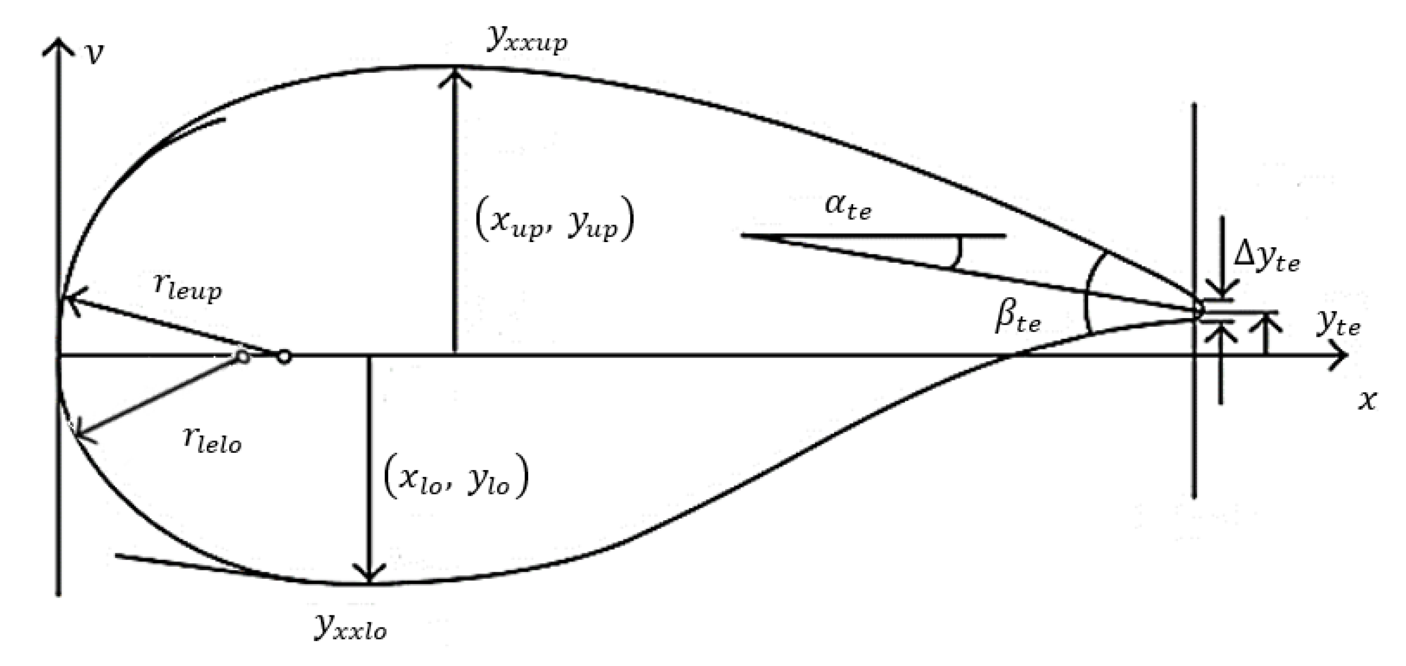
Figure 2.
Parameter design variable of the airfoil for parameter section (PARSEC) parametrization.

Figure 3.
NREL S809 airfoil generated by PARSEC parameterization.

Figure 4.
Optimized airfoil shape profile by a genetic algorithm (GA).

Figure 5.
Optimization flow chart elaborating on the MATLAB code for airfoil shape optimization.

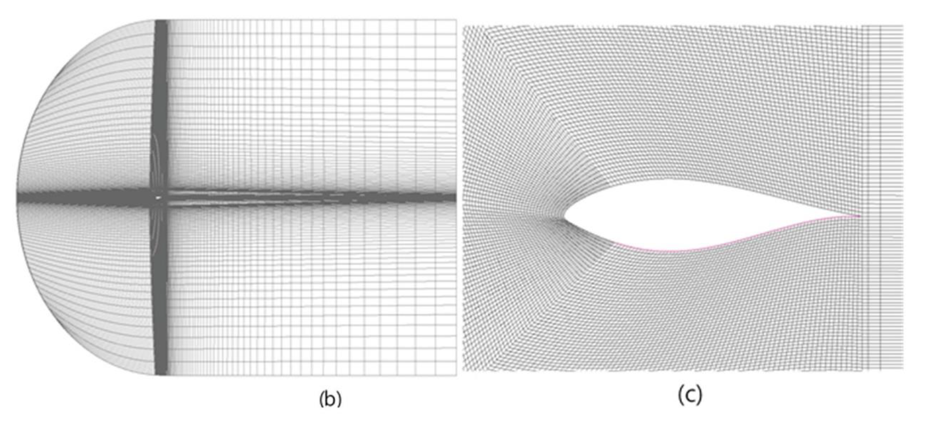
Figure 6.
The C-type mesh for the baseline airfoil of a wind turbine at an angle of attack (AOA) of 6.2°. (a) Overall blocking structure; (c) the mesh; and (b) zoomed-in mesh image.
Figure 6.
The C-type mesh for the baseline airfoil of a wind turbine at an angle of attack (AOA) of 6.2°. (a) Overall blocking structure; (c) the mesh; and (b) zoomed-in mesh image.


Figure 7.
Mesh distribution of the airfoil at AOA = 6.2°.

Figure 8.
Mesh topology structure and its name.

Figure 9.
Shape comparison of the baseline and optimized airfoils (NREL S-809).

Figure 10.
Variation of lift coefficient with the angle of attack for the S809 airfoil.

Figure 11.
Variation of drag coefficient with the angle of attack for the S809 airfoil.

Figure 12.
Pressure distribution curve over the NREL S809 airfoil.

Figure 13.
The convergence graph with the iterations for the NREL S809 airfoil via (a) the CST method and (b) the PARSEC method.
Figure 13.
The convergence graph with the iterations for the NREL S809 airfoil via (a) the CST method and (b) the PARSEC method.

Figure 14.
Pressure distribution curve plot between the experimental and CFD S809 airfoils.

Figure 15.
Pressure contour at 0° (left) and 6.2° (right) for the (a) baseline S809 airfoil and (b) optimized S809 airfoil.
Figure 15.
Pressure contour at 0° (left) and 6.2° (right) for the (a) baseline S809 airfoil and (b) optimized S809 airfoil.

Figure 16.
Velocity contour at 0° (left) and 6.2° (right) for the (a) baseline S809 airfoil and (b) optimized S809 airfoil.
Figure 16.
Velocity contour at 0° (left) and 6.2° (right) for the (a) baseline S809 airfoil and (b) optimized S809 airfoil.


Table 1.
The twelve basic airfoil for parameter section (PARSEC) parameters.
| PARSEC Parameter | Geometric Parameter | Definition |
|---|---|---|
| Upper leading edge radius | ||
| Lower leading edge radius | ||
| Upper crest position in horizontal coordinates | ||
| Upper crest position in vertical coordinates | ||
| Upper crest curvature | ||
| Lower crest position in horizontal coordinates | ||
| Lower crest position in vertical coordinates | ||
| Lower crest curvature | ||
| Trailing edge offset in a vertical sense | ||
| Trailing edge thickness | ||
| Trailing edge direction | ||
| Trailing edge wedge angle |
Table 2.
Optimization criteria and constraints.
| Geometric Constraints | Trailing edge offset in a vertical sense and trailing edge thickness are kept zero |
| Aerodynamic Constraints | Lift coefficient should be greater than the original airfoil Wind angle of attack = and |
| Objective | Maximize lift coefficient () and lift-to-drag ratio (L/D) |
| Termination Criteria | No change in maximum fitness value for 20 generations |
Table 3.
Operating parameters for the airfoil.
| Boundary Condition | Velocity of Flow (u) | Mach Number (M) | Reynolds Number (Re) | Angle of Attack (°) | Dynamic Viscosity (μ) | Density ρ | Chord Length (c) | Temperature (T) | Gas Constant (R) | Working Fluid | Pressure (P) |
|---|---|---|---|---|---|---|---|---|---|---|---|
| Units | |||||||||||
| NREL S809 | 7 | 0.02 | 0 & 6.2 | 1.258 | 0.34 | 288 | 287 | Air |
Table 4.
Distribution of mesh in the computational domain for the mesh independence study.
| Mesh | Nodes along the Upward Direction | Nodes in Front of the Leading Edge | Nodes along the Downward Direction | Nodes along the Airfoil Length | Face Diagonal Nodes | Nodes along the Trailing Edge | Nodes along the Leading Edge | Maximum Value of y+ | Coefficient of Drag (Cd) | Coefficient of Lift (Cl) | Total Number of Nodes (Millions) | Memory Allocated by the Solver | CPU Time for 10 Iterations |
|---|---|---|---|---|---|---|---|---|---|---|---|---|---|
| M-i | [MB] | [s] | |||||||||||
| M1 | 125 | 75 | 125 | 75 | 75 | 250 | 150 | 0.7 | 0.0174 | 0.963 | 3.6 | 595 | 68 |
| M2 | 125 | 100 | 125 | 75 | 100 | 300 | 200 | 0.7 | 0.0156 | 0.973 | 4.9 | 796 | 95 |
| M3 | 125 | 125 | 125 | 75 | 125 | 350 | 250 | 0.7 | 0.0147 | 0.985 | 6.3 | 1023 | 122 |
| M4 | 125 | 150 | 125 | 75 | 150 | 400 | 300 | 0.7 | 0.0146 | 0.985 | 8 | 1278 | 157 |
Table 5.
The design parameters for the NREL S809 airfoil.
| Variables | CST Parameters | Variables | PARSEC Parameters |
|---|---|---|---|
| −0.1112 | P1 = rleup | 0.0216 | |
| −0.4286 | P2 = rlelo | 0.010 | |
| −0.2461 | P3 = Xup | 0.3826 | |
| 0.0525 | P4 = Yup | 0.1018 | |
| 0.1682 | P5 = YXXup | −1.201 | |
| 0.3288 | P6 = Xlow | 0.3633 | |
| 0.2567 | P7 = Ylow | −0.1081 | |
| 0.1788 | P8 = YXXlow | 1.526 | |
| P9 = yte | 0 | ||
| P10 = delta yte | 0 | ||
| P11 = alpha te | 8.5 | ||
| P12 = beta te | 8.5 |
Table 6.
Performance comparison of the original and optimized airfoils (NREL S-809).
| NREL S-809 | Relative Variation | ||||
|---|---|---|---|---|---|
| Experimental Data (OSU) | Optimized Airfoil (CST Method) | Optimized Airfoil (PARSEC Method) | CST with Experimental Data | PARSEC with Experimental Data | |
| 0.79 | 0.883 | 0.87 | +11.8% | +10.1% | |
| 0.0131 | 0.0134 | 0.0148 | −2.2% | −12.1% | |
| L/D | 60.3 | 65.9 | 58.8 | +9.6% | −2.0 % |
| AOA | 6.2° | 6.2° | 6.2° | ||
Table 7.
Comparison of simulation data of the original and optimized airfoils by CFD (NREL S809).
| Baseline Airfoil (Experimental) | Optimized Airfoil (CFD) | Relative Variation | |
|---|---|---|---|
| 0.79 | 0.985 | +24.6% | |
| 0.0131 | 0.0147 | +12.2% | |
| L/D | 60.3 | 67 | +12.4% |
| AOA (°) | 6.2° | 6.2° |
Publisher’s Note: MDPI stays neutral with regard to jurisdictional claims in published maps and institutional affiliations. |
© 2021 by the authors. Licensee MDPI, Basel, Switzerland. This article is an open access article distributed under the terms and conditions of the Creative Commons Attribution (CC BY) license (http://creativecommons.org/licenses/by/4.0/).
Share and Cite
MDPI and ACS Style
Akram, M.T.; Kim, M.-H. Aerodynamic Shape Optimization of NREL S809 Airfoil for Wind Turbine Blades Using Reynolds-Averaged Navier Stokes Model—Part II. Appl. Sci. 2021, 11, 2211. https://doi.org/10.3390/app11052211
AMA Style
Akram MT, Kim M-H. Aerodynamic Shape Optimization of NREL S809 Airfoil for Wind Turbine Blades Using Reynolds-Averaged Navier Stokes Model—Part II. Applied Sciences. 2021; 11(5):2211. https://doi.org/10.3390/app11052211
Chicago/Turabian StyleAkram, Md Tausif, and Man-Hoe Kim. 2021. "Aerodynamic Shape Optimization of NREL S809 Airfoil for Wind Turbine Blades Using Reynolds-Averaged Navier Stokes Model—Part II" Applied Sciences 11, no. 5: 2211. https://doi.org/10.3390/app11052211
Note that from the first issue of 2016, this journal uses article numbers instead of page numbers. See further details here.