
Data Augmentation Using Generative Adversarial Network for Automatic Machine Fault Detection Based on Vibration Signals


Department of Electronics Engineering, Kookmin University, Seoul 02707, Korea
*
Author to whom correspondence should be addressed.
Appl. Sci. 2021, 11(5), 2166; https://doi.org/10.3390/app11052166
Submission received: 2 February 2021
/
Revised: 22 February 2021
/
Accepted: 25 February 2021
/
Published: 1 March 2021
(This article belongs to the Collection Machine Learning in Computer Engineering Applications)
Abstract
:In the last decade, predictive maintenance has attracted a lot of attention in industrial factories because of its wide use of the Internet of Things and artificial intelligence algorithms for data management. However, in the early phases where the abnormal and faulty machines rarely appeared in factories, there were limited sets of machine fault samples. With limited fault samples, it is difficult to perform a training process for fault classification due to the imbalance of input data. Therefore, data augmentation was required to increase the accuracy of the learning model. However, there were limited methods to generate and evaluate the data applied for data analysis. In this paper, we introduce a method of using the generative adversarial network as the fault signal augmentation method to enrich the dataset. The enhanced data set could increase the accuracy of the machine fault detection model in the training process. We also performed fault detection using a variety of preprocessing approaches and classified the models to evaluate the similarities between the generated data and authentic data. The generated fault data has high similarity with the original data and it significantly improves the accuracy of the model. The accuracy of fault machine detection reaches 99.41% with 20% original fault machine data set and 93.1% with 0% original fault machine data set (only use generate data only). Based on this, we concluded that the generated data could be used to mix with original data and improve the model performance.
1. Introduction
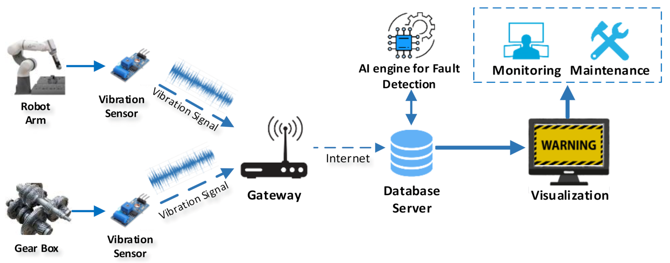
Machine maintenance is one of the most important fields in the industrial environment. In the normal working condition, the maintenance costs range from 15% to 40% of the total production cost [1]. Most manufacturing industries today use preventive maintenance, which replaces the machine parts based on a fixed schedule, to guarantee high maintenance safety. However, preventive maintenance cannot be considered as an effective maintenance method because the fixed schedule could not make full use of resources. This method can save costs ranging from 8% to 12% of the traditional maintenance cost and 40% of the reactive maintenance cost [2]. In the last decade, predictive maintenance has a more and more important role in manufacturing because of the improvement of the Internet of Things (IoT) and real-time data management. In the modern industrial environment, predictive maintenance focuses on the IoT and artificial intelligence (AI) platforms. In Figure 1, the maintenance includes data collection and signal processing to conducts early fault detection and diagnosis. Based on these platforms, the system can perform data collection and signal processing to conducts early fault detection and diagnosis by applying the concepts of data collection and management [3]. Some signal are popular in machine fault detection, such as vibration and acoustic signal. However, the acoustic signal is harder to collected, and more sensitive to noise, compared to vibration signal [4]. Various predictive maintenance schemes and AI models, which mostly use supervised learning, have been proposed lately [5,6].
However, in the early phases when abnormal operations and fault machines rarely appeared in real-time scenarios, the initial fault vibration samples set is restricted. In the case of absent or limited fault samples, the training process for fault classification applications is difficult to conduct because of the imbalance of the input data. Therefore, data augmentation is necessary to increase the performance of the model training process when dealing with small fault datasets. An approach for the limited training data is transfer learning, where the target signal is created based on the source signal, which has the same distribution [7,8]. However, the source signal using for transfer learning also requires the balance between the normal and fault data set. Therefore, data augmentation is also necessary for the transfer learning techniques when dealing with small fault datasets at the initial phase. In practice, the works of data augmentation in the time-series region are very limited and mostly focus on the traditional data transformation methods. The example of these methods is jittering [9,10], scaling [9,10], window slicing [10,11], and flipping [10,12,13]. In these studies, the traditional data transformation methods do not significantly improve the accuracy of the model [9,10,11,14]. Data augmentation, therefore, is not fully evaluated in time-series data analysis and fault detection applications. With the increase in the demand for fault detection applications in smart factories, the requirement for effective methods for data augmentation has been increasing [9,15].
The general generative models produce outputs similar to the samples in the training dataset [16] by mimic the probability distribution function of the original data. The most popular generative method in data augmentation is the generative adversarial network (GAN) [17,18]. The GAN algorithm is mostly applied in image processing and image generation. The main drawback of GAN is its instability during the training process, where the discriminator and generator try to fool each other [19]. Several studies have been conducted to improve GAN stability in the training process [20]. However, the limitation in GAN evaluation required human inspection, especially for picture generation and computer vision.
In this paper, vibration data from Spectra Quest’s Gearbox Prognostics Simulator (GPS) is tested using various fault detection approaches for both limited and unlimited input data. Another data source that can be considered is the real-scenario data, such as Reference [21]. However, the experiments are not compatible with the GPS dataset, and the measurement is not conducted thoroughly. Therefore, we only consider using the GPS dataset for the data augmentation in this study. Using GAN, we generate the broken signal to improve the training performance of the model. Using different approaches in both the experiment and test, we evaluated the generated data comprehensively and avoided misjudging during the data generation process for obtaining the final results. Our main contributions in this paper are as follows:
- We briefly review the characteristic of the vibration signal data with different approaches in fault detection applications. These approaches are mainly used to verify that the generated data are high quality and suitable for fault detection applications.
- We introduce GAN algorithms to generate a broken machine signal, which has high quality and is similar to the original signal.
- The main contribution of this paper is the different approaches used to evaluate the generation data and to guarantee similarity with the original data. These approaches include different preprocessing processes and a variety of machine learning techniques in pattern recognition.
The remainder of this paper is organized as follows. Section 2 describes the fault diagnosis input data and the Fast Fourier Transform (FFT), which provides the refined signal for further data processing and classification. Section 3 provides the working scheme with real data, which includes the full signal, principal component analysis (PCA) transform, and statistical analysis (SA). We also introduce different machine learning techniques for each approach and perform a comprehensive analysis. We discuss data generation using GAN and compare it with the original data in Section 4. With various preprocessing approaches and AI models, the generated data is evaluated carefully with high similarity with the real data. Conclusions for the data augmentation using GAN are presented in Section 5.
2. Vibration Data and Early Data Processing
2.1. Gearbox Data
The vibration signal used in this study is collected from the GPS and then uploaded to OpenEI data storage [22]. The GPS simulates a real gearbox device and has configurations with different options and working behaviors. Based on these configurations, the GPS can simulate gearbox working behavior, condition monitoring, and vibration data for further study.
The basic GPS includes replaceable parts that are combined for gearbox operation simulation as follows:
- one shaft test gearbox with two parallel stages;
- different torsion and radial loadings;
- replaceable gears with large spaces for additional devices;
- parallel gearbox that can support rolling element bearings or sleeve bearings;
- option for installing intentional error gearing to study the changes in the vibration signature;
- modular design that keeps the simulation easy to understand and doable;
- different mounting locations; and
- gearbox fault simulation and diagnosis methods.
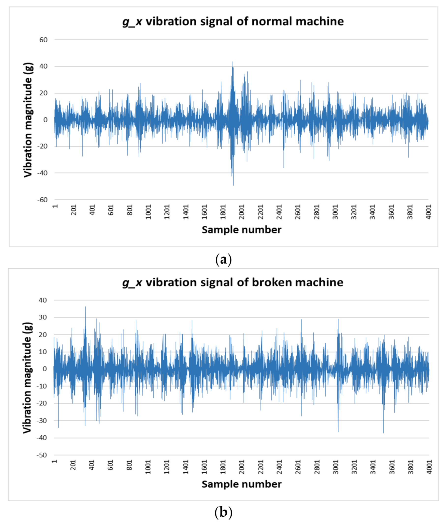
Based on these characteristics, the GPS can be customized to handle and examine heavy loads. GPS is also designed with a large reserve space so that the users can place, set up, and install new monitoring devices. In this paper, we collected data in the four directions: g_x, g_y, g_z, and g_t. In Figure 2, the GPS is set at 50% of the load condition, and we record the vibration signal under normal conditions and the broken tooth condition. The GPS data includes 450 s of normal machine vibration signal and 400 s of broken machine vibration signal.
2.2. Fast Fourier Transform
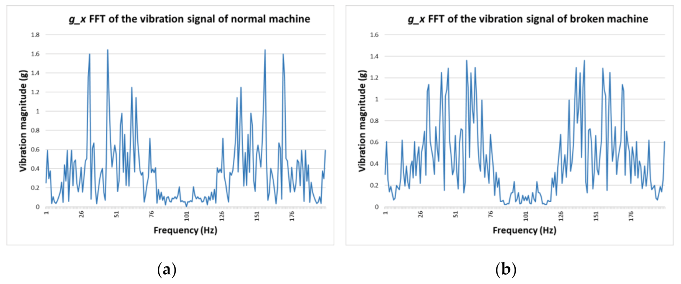
In the first phase, we extract significant characteristics of the input signal by performing feature extraction. These characteristics vary from signal to signal and are statistical, domain-specific features, or both. In Figure 2, the vibration data are collected and stored as the time series, and we transform it into the frequency domain using Fast Fourier Transform (FFT) (Figure 3). The main purpose of this study is to generate and evaluate broken data that is limited in the experiments. Therefore, we need to analyze both the original and generated data with different approaches and AI models that can affect final results.
The Fourier Transform is a function of frequency, which has the magnitude to represent the frequency in the time domain. The Fourier Transform can vary in the domains, but the original function is mostly considered as the time domain. The definition of the Fourier Transform of a Discrete Function is as follows.
Let x0, …, xN−1 be complex numbers. We can calculate the Discrete Fourier Transform (DFT) in the time domain by using the following formula:
where x0,…, xN−1 are complex numbers, and is a primitive N-th root of 1 [23].
For FFT, the formula changes into the following expression:
By transforming Formula (1) into Formula (2) and (3), the Fourier Transform is split into two smaller transforms with odd-numbered values and even-numbered values. At this point, we did not decrease the computational complexity, which consists of 2 × [(N/2) × N], for a total of N2.
With the symmetrical characteristics of Formulas (2) and (3), we can reduce the number of computations. The value of k is defined as 0 ≤ k < N, whereas the value of n is 0 ≤ n < M ≡ N/2; each sub-problem required half the computation of the original one. The total computation is reduced from O[N2] to O[(N/2)2] [24].
The FFT requires lower computation as compared with the original FFT, which is suitable for real-time applications. In this study, we focus on the commercial application in the industrial environment, which requires both high accuracy and real scenario response. Due to these reasons, FFT would be a better choice compared to the DFT. The advantage of FFT is that we can process more significant features in the frequency domain classification between the normal and broken machine signals. Another advantage of the FFT transform is that the generated signal is evaluated indirectly, which leads to better performance analysis. We can consider FFT as one of the most effective methods used to extract the vibration input pattern [5]. Therefore, we use FFT as the basic processing method for further research. Based on the FFT input signal, we propose three approaches: full analysis, PCA transform, and statistical analysis. In the next section, we will discuss different approaches and AI models that can be applied to the fault diagnosis results.
3. Fault Diagnosis with Original Data
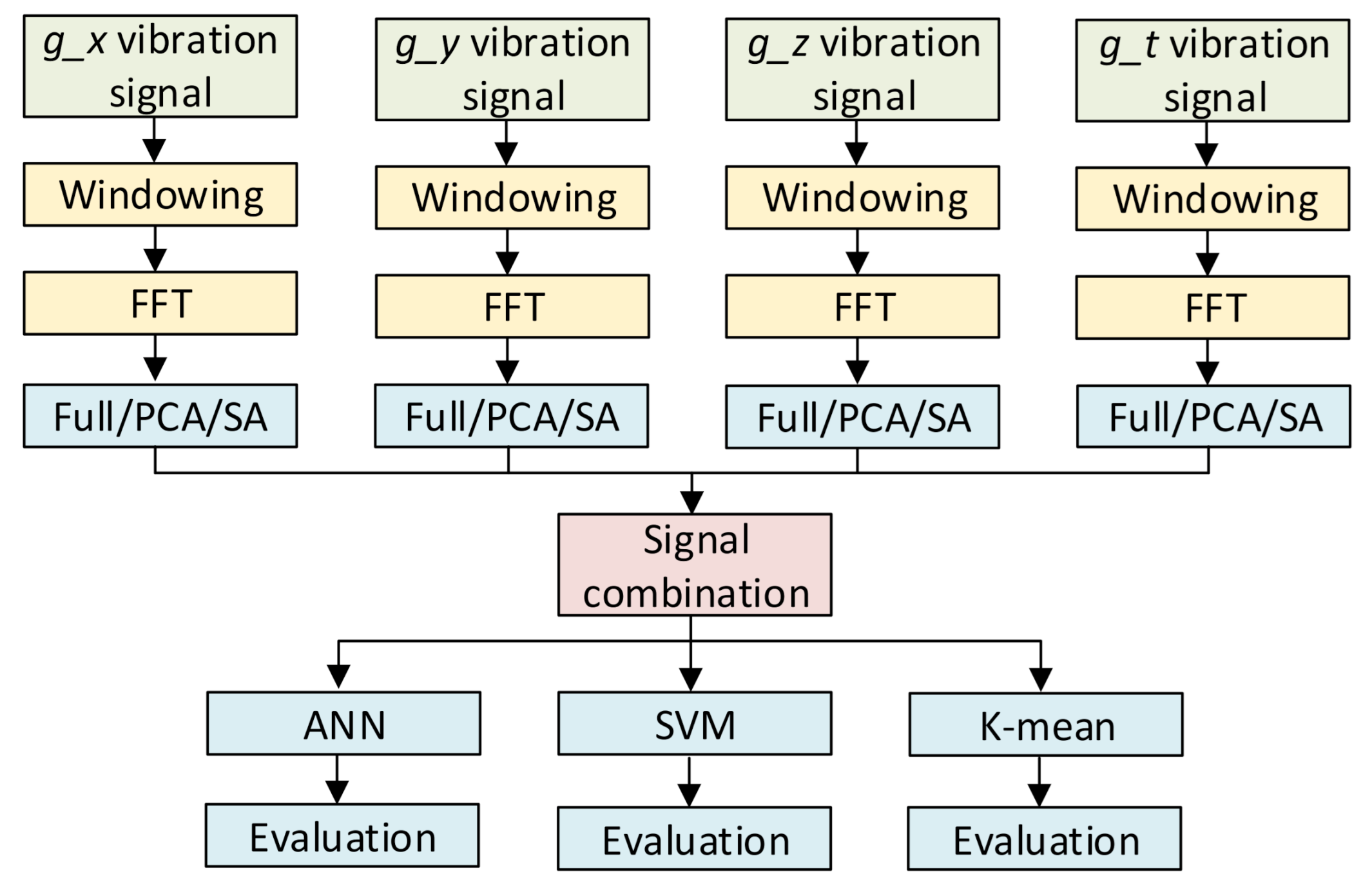
In general, data augmentation is mostly used in image processing [15] because it is easy to evaluate whether the generated data is similar to the original data based on the judgement of human. In contrast, it is difficult to evaluate the data augmentation in data analysis because it depends on a different characteristic of the data. Therefore, to evaluate the generation data, we require a comprehensive test with various conditions. This section introduces three fault detection approaches for vibration signals, which can be applied to the generated signal. The overall fault diagnosis diagram with different data processing and multiple AI models is shown in Figure 4. The vibration data in each direction is windowed and transformed into the frequency domain for further process. Then, we provide 3 different methods for feature extractions, includes full analysis, PCA transform, and statistical analysis. After that, all four signal is combined and feed to different AI algorithms, includes artificial neural network (ANN), support vector machine (SVM), and K-mean clustering. All the approaches introduced in this section will be the basis for further analysis and evaluations.
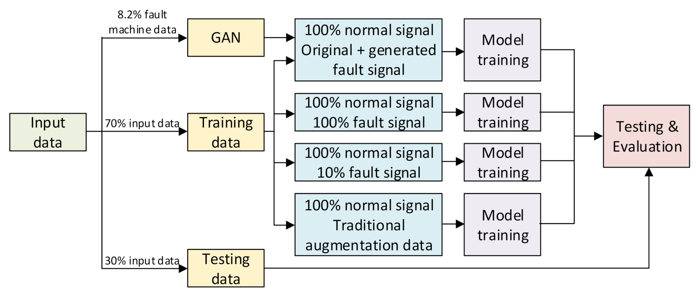
Figure 5 introduces the training and testing process using both generated data by GAN and real data. The input data is divided into 3 groups: training data includes 70% of total data, testing data includes 30% of total data, and GAN data includes 11.75% data of fault machine of the training data (8.2% of total fault machine data).
3.1. Full Analysis and PCA Transform
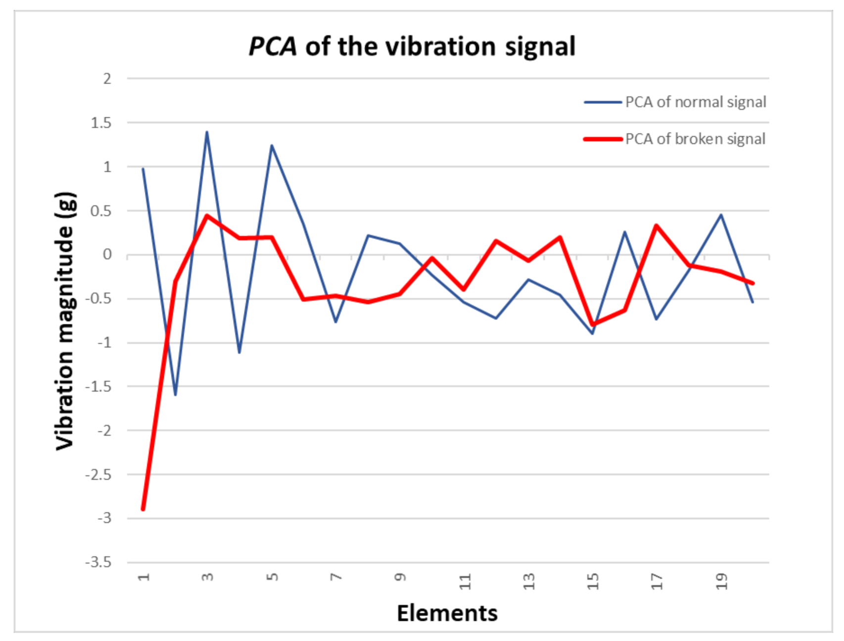
In this approach, the FFT of the signal is fed directly into the AI model to determine whether or not the machine has errors. The AI models analyzed in this study are artificial neural network (ANN) [25], K-mean clustering [26], and support vector machines (SVM) [27]. These models have proved to be robust for classification applications. Moreover, ANN, K-mean clustering, and SVM are very flexible when dual with different data types and structures. However, K-mean clustering and SVM-based models are not effective when applied with high-dimension input data [28]. Therefore, we also consider the PCA to reduce the dimensions of the input data. Figure 6 shows normal and broken sample data of the signal after the PCA process, which transforms high-dimension input data into low-dimension input data for K-mean clustering and SVM algorithms.
The vibration signals, which include full FFT and PCA transform, are fed into the ANN networks. The inputs are different so we consider two ANN structures for the machine fault detection application. The first ANN model for the full FFT of the signal has a large structure because the input contains all four signals in the g_x, g_y, g_z, and g_t directions. This ANN model has an input shape of 200 × 4, 200 input neural, 100 hidden units, and 2 output neural with the Softmax activation function for classification. The Softmax function is defined as follows:
where i = 1,…, K and z = (z1,…,zK). The predicted probability of an output of the neural network classified as normal (or broken machine) is:
where x is the input vector; w is the weighting vector of the output neural network; and xTw is the inner product of x and w. In this formula, we have i = 1,…,K and z = (z1,…,zK).
The PCA transform reduces the FFT of the signal into a 20 × 1 vector, which is much smaller than the original signal. Therefore, the ANN has a small structure with 64 input neural, 32 hidden units, and 2 output neural with the Softmax activation function for classification. For comparison, we apply the same optimization for both the ANN structures. Xavier initialization [29] is applied to set up the weights of all ANN cells, and the Dropout technique [30] with 0.7 keeping probability is also used to improve the ANN performance. We use Leaky Rectified Linear Unit (Leaky ReLU) [31] as the activation function for both the input and hidden layers, which is defined as follows:
Sparse categorical cross-entropy is used as the loss function for our ANN models, and Adaptive Moment Estimation (ADAM) is selected as the optimization algorithm with 1000 epochs.
Table 1 shows the accuracy of ANN, K-mean clustering, and SVM based on two input data (full FFT of the signal and PCA transform signal). The accuracy of ANN, K-mean clustering, and SVM reaches 100% in both cases. Compared with the acoustic signal in Reference [4], we achieve higher accuracy with a simpler data collection method. However, with high training and testing speed, the K-mean clustering and SVM are more suitable in the real-time scenario. Table 2 shows the test results with a small broken machine signal training set (40 s of broken signal, only 10% of the original amount). When there is a lack of small broken machine signal data, the accuracy drops significantly as compared with the original condition. Table 3 shows the result with traditional data augmentation, includes jittering, scaling, and slicing. The accuracy improves slightly as compared with Table 2, which shows that this method cannot significantly improve the performance of the model.
3.2. Statistical Analysis
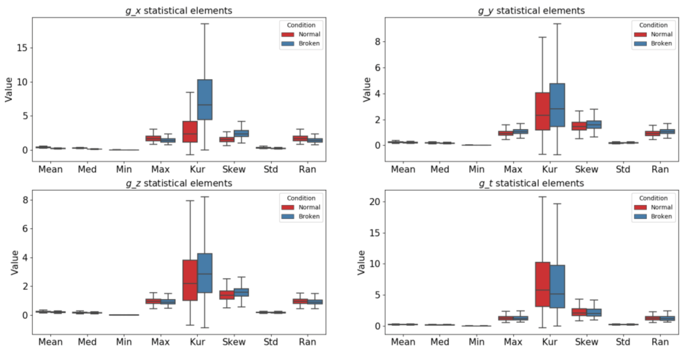
The third approach is that of statistical analysis, which uses the extracted features from the FFT of the signal. The FFT of the signal is analyzed based on the statistical features that have eight parameters: mean, median, min, max, kurtosis, skewness, standard deviation, and range. These features are obtained along all four axes: g_x, g_y, g_z, and g_t. Each data sample contains 32 elements. Due to low input data dimensions, these approaches are suitable with ANN, K-mean clustering, and SVM. The statistical approach not only provides another efficient method for fault classification but also plays an important role in evaluating the generated data. Using statistical analysis, we extract the overall characteristics of the vibration signal. Based on these characteristics, we can compare the generated data with the original data. If the generated data has high accuracy in the statistical analysis, we can conclude that it has a high similarity level with the original data and can be used for the training process. Before feeding data into the AI models, we should understand the variations in the statistical characteristics of the FFT of the signal.
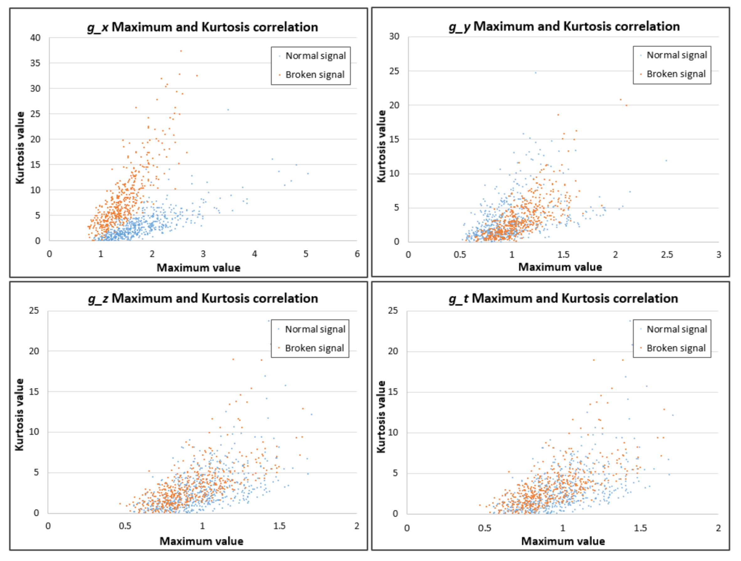
The statistical relationship between the normal and broken machine signals can be considered a reliable classification method, as shown in Figure 7. The statistical elements of the normal and broken signal are similar in the g_y, g_z, and g_t directions, but they are different in the g_x direction. The most difference is seen in the maximum value (4) and kurtosis value (5) of the g_x signal. In Figure 8, if we break down the relationship between them, we can easily classify the normal and broken machine signals.
The performance of ANN, K-mean clustering, and SVM based on statistical analysis are shown in Table 4. The ANN algorithm reaches over 95% accuracy in three scenarios, which proves that robust classification features were adopted. In contrast, K-mean clustering and SVM have the worst performance as compared with full FFT analysis. In the classification using real data, K-mean clustering and SVM showed poor performance as compared with a full analysis approach. However, this characteristic can be used to analyze the performance of the generated data for an unstable classification method. This approach needs to be considered when the generated data is used.
4. Data Generation in Machine Fault Detection
In the previous section, we concluded that the lack of vibration signals in the training process will decrease the accuracy of the predictive models, regardless of the kind of data process. To improve the accuracy of the predictive model, we introduce data augmentation using GAN to generate broken data similar to the original data. Data generation is based on the original data of the vibration signal of the broken machine, which includes 47 sof vibration and uses 11.75% of the normal signal. The generated signal is analyzed based on the approaches described in Section 3. With different approaches and AI models, we can guarantee the evaluation process with high accuracy and similarity with the original data, which can help to improve the predictive model.
4.1. GAN
GAN is a technique designed by Ian Goodfellow to generate new data from a fixed training data set. In this technique, the discriminative and the generative neural networks compete in a zero-sum game to improve themselves. Using a limited training set, the GAN techniques learn by themselves to generate data using the specific structure. The most well-known GAN applications are those in computer vision, in which a photograph set is trained to generate new output with realistic characteristics for human observers. Although previous studies were mostly focused on unsupervised learning, GANs were then used in semi-supervised learning and reinforcement learning. The core idea is to “indirectly” train a generator using the discriminator. Based on this idea, the generator is trained to fool the discriminator but not to minimize the total loss of the function, which leads to the ability to generate new data in a different manner.
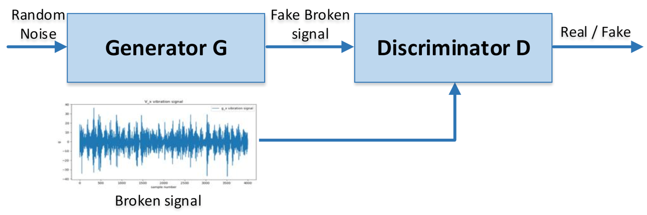
GAN was first proposed in Reference [33] to generate images similar to the original image. In a practical situation, GAN can be considered as the competition between a discriminative network D and a generative network G. With normal contribution or random noise, which ranges from 0 to 1 as the input, the generative network G generates the “fake” data G(z), in which distribution pg is close to that of the data distribution pdata. The role of the discriminative network D is to distinguish the true data sample x ∼ pdata(x) and the generated sample G(z) ∼ pg(G(z)). In the original GAN, this adversarial training process was formulated as follows:
The adversarial procedure is illustrated in Figure 9. Most existing GANs perform a similar adversarial procedure in different adversarial objective functions. In this paper, the GAN algorithm is used to generate the broken machine data signal; therefore, only broken training data is fed into the generator. The generator generates the broken data using random noise, which ranges from 0 to 1 with normal distribution to guarantee the difference in the output data.
The generator G and discriminator D have the ANN structure and are implemented as shown in Table 5 and Table 6, respectively. The generator G has a complex structure to generate a broken high-quality signal, whereas the discriminator D has a simpler structure for classification. Note that the output of the generator G has the same shape as the input, whereas the output of the discriminator D is a single value between 0 and 1 because the sigmoid activation function for classification is applied.
4.2. Data Generating
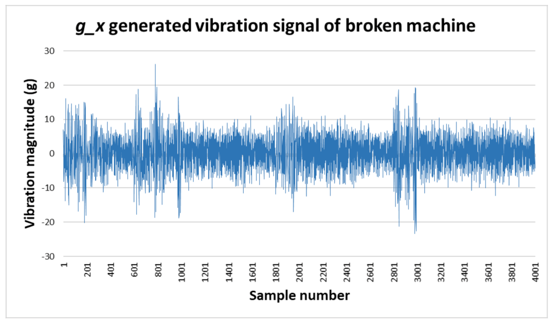
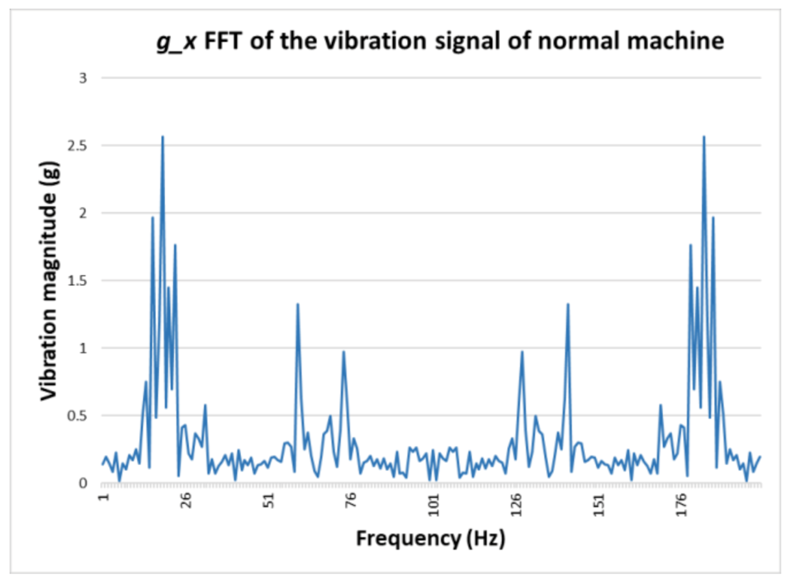
The data generated using GAN includes 500 s of vibration signals, which includes the four signals g_x, g_y, g_z, and g_t. The generated broken signal is shown in Figure 10, which contains the individual g_x vibration signal. The preprocessing procedure for the generated signal is the same as that for the original signal, and, based on that, we can evaluate its quality using previous fault detection methods. Note that we generate the signal only for the broken machine because the broken signal is assumed to be less than the signal obtained for the original data. The FFT of the g_x signal is calculated and shown in Figure 11.
4.3. Fault Diagnosis Using Generated Signal
Based on both the original and generated data, we evaluated the final results using the three approaches described in Section 3. Keeping the same testing data, we simulated the actual situation of the AI model in real life. In contrast, the training data is a mix of the real data and the generated data. The ratio of the real data over generated data is 100%, 80%, 60%, 40%, 20%, and 0%. With this testing condition, different signal processing approaches, and AI model, the generated data will be evaluated comprehensively if it can satisfy the data augmentation requirement in a fault machine detection application.
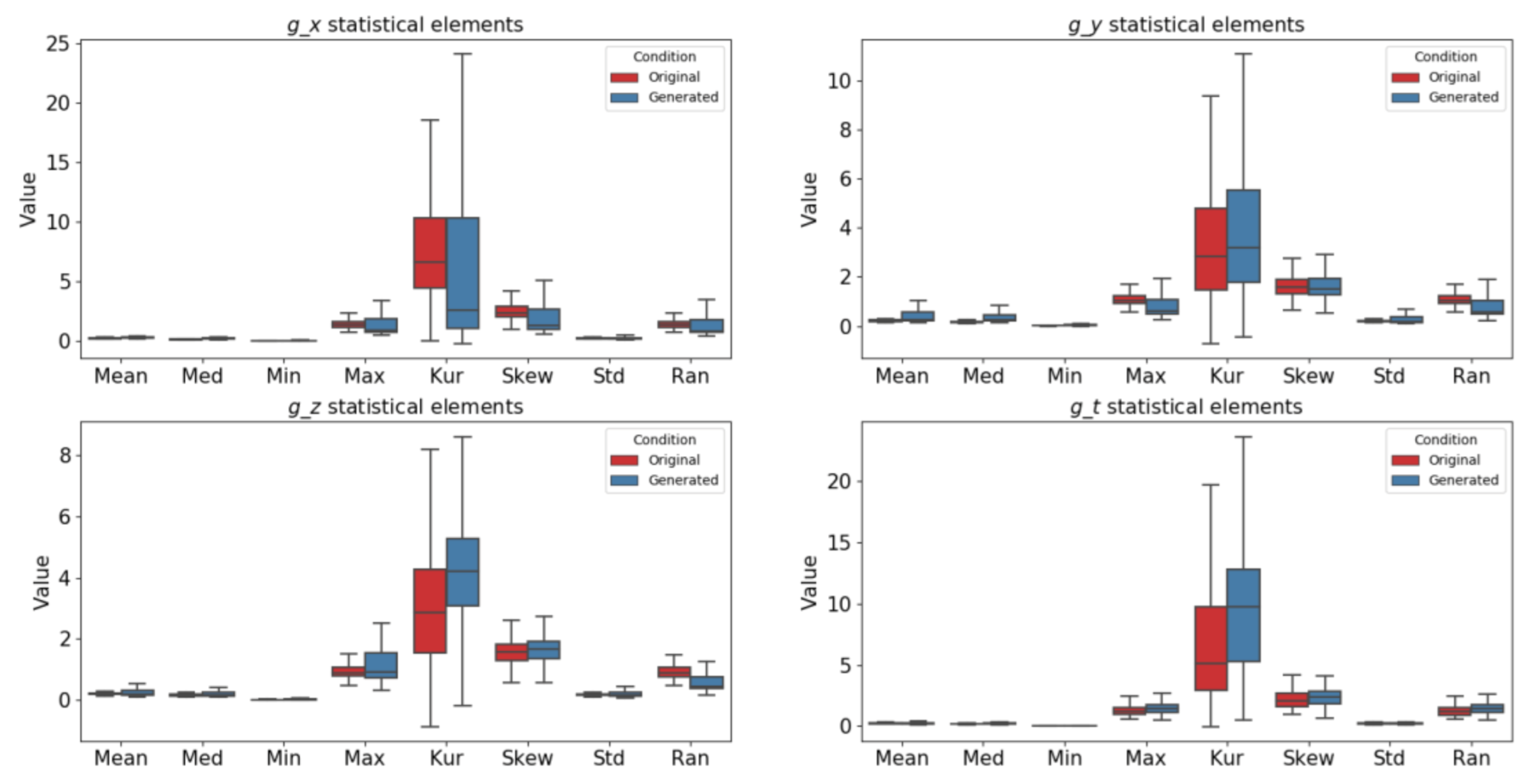
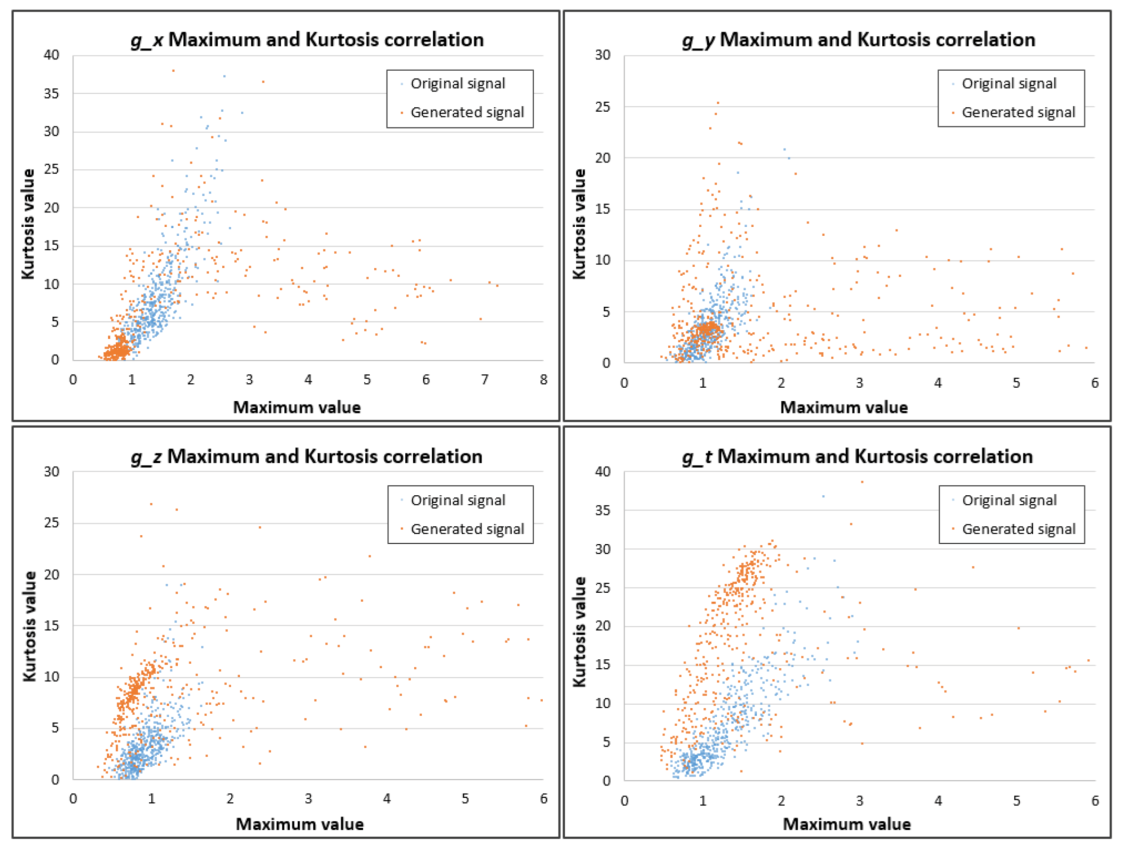
To verify the similarity between original data and generated data, we conducted the Kolmogorov-Smirnov test using Python version 3.7.4 [34]. The statistic value is 0.059, while the p-value is 0.336, so we can accept the hypothesis that signals are drawn from the same distribution. Figure 12 illustrates the relationship among all statistical elements between an original broken machine signal and a generated signal. The generated signal has a larger data variation distribution with taller boxed, which shows the variations during the generation phase. In Figure 13, by continuing to break down the relationship between the maximum and kurtosis values of the original and generated broken FFT of the signals, we can see high variations in the generated values. The linear regression test [35] is conducted to verify the correlation between the maximum and kurtosis values. The coefficient of determination is calculated and shown in Table 7. With the high value of Coefficient of Determination in all dimension g_x, g_y, g_z, and g_t, we can conclude that the maximum and kurtosis has a high correlation in fault signal. Compared with the original signal, the generated signal has a lower Coefficient of Determination, indicating that it has higher variation and less dependent on each other. This variation is good for the training phase because it can improve the machine learning models with different input patterns.
Table 8 shows the accuracies of ANN, K-mean clustering, and SVM with different approaches based on the FFT of the vibration signal. With the full FFT of the signal approach, the data augmentation with the original data larger than 40% worked well under the testing condition with 100% accuracy (ANN). This result is better than the 0% original data set, which has the accuracy of 89.4% (ANN), 60.2% (K-mean clustering), and 93.1% (SVM). The classification algorithms worked much better in the case where 20% original data were used, which achieve the accuracy of 95.1% (ANN), 61.3% (K-mean clustering), and 95.3% (SVM). In the case of using PCA transform for the FFT signal, the data augmentation with the original data larger than 40% worked well under the testing condition with 98.1% accuracy (ANN). This result is better than the 0% original data set, which has the accuracy of 87.2% (ANN), 55.3% (K-mean clustering), and 91.0% (SVM). The classification algorithms worked much better in the case where 20% original data were used, which achieve the accuracy of 93.1% (ANN), 65.2% (K-mean clustering), and 94.7% (SVM). In the last approach, the statistical analysis of the FFT of the signal, the ANN provides almost 100% accuracy with more than 20% original data. The accuracy of the ANN algorithm decreases to 79.41% when there is 0% original data; this is much better than the traditional augmentation method in Section 3. In this approach, the K-mean clustering and SVM have poor performance as compared with ANN. The SVM has high accuracy and stable with different test sets, so it is strong enough to be considered in real-life scenarios. In contrast, the K-mean clustering is not stable and requires more accuracy to be considered as a reliable classification approach. The result shown in Table 8 indicates that the general data have high similarity as compared with the original data in the FFT of the signal and can be replaced in the training process.
Data augmentation is useful in the training process when the number of fault samples is so small that the model cannot be trained effectively. This characteristic is very suitable in machine fault detection because of the lack of fault machines at the start of the implementation phase. With the improvement of GAN, we can generate fault data for applying the machine fault diagnosis with high similarity to the original data. Using various experiments and evaluations, we can conclude that the generated data has a high similarity with the original data in both the time domain and frequency domain. The generation data significantly improved the application of training performance with a large machine fault sample. Although we could generate high-quality input data, the original fault data are also necessary for testing and partial training.
5. Conclusions
This study proposed a novel method to generate the fault machine vibration signal data, thus enhancing the model performance in the case of a limited fault dataset for training. In this study, our generated fault data improve the accuracy of the model to 93.1% with 0% original fault machine data set (Full signal analysis) and 99.41% with 20% original fault machine data set (statistical analysis). After testing, we conclude that the generated data has high similarity to the original data and significantly improves the accuracy of the model with limited real fault machine data in the training dataset.
However, the data augmentation method using GAN still has a limitation, since the high variety can reduce the output signal. Another drawback of GAN is unstable during the training process, in which the balance between the discriminator and the generator needs to be maintained. Therefore, the architectures of both the generator and discriminator should be considered carefully, and the output of GAN has to be carefully evaluated.
With the disadvantages of GAN, we consider to provide other generative AI models for the data augmentation and compare with the current scheme. Another option is to provide a model to generate the fault data for different machines, only using the fault data of one machine and normal data of other machines.
Author Contributions
Conceptualization, V.B. and T.L.P.; methodology, V.B.; software, V.B. and H.N.; validation, V.B., T.L.P., and H.N.; formal analysis, V.B.; resources, V.B.; writing—original draft preparation, V.B.; writing—review and editing, T.L.P. and Y.M.J.; supervision, Y.M.J.; project administration, V.B.; funding acquisition, Y.M.J. All authors have read and agreed to the published version of the manuscript.
Funding
This research was financially supported by the Ministry of Trade, Industry and Energy (MOTIE) and Korea Institute for Advancement of Technology (KIAT) through the International Cooperative R&D program (Project ID: P0011880).
Institutional Review Board Statement
Not applicable.
Informed Consent Statement
Not applicable.
Data Availability Statement
Data available in a publicly accessible repository that does not issue DOIs. Publicly available datasets were analyzed in this study. This data can be found here: [https://openei.org/datasets/dataset/gearbox-fault-diagnosis-data (accessed on 15 January 2021)].
Conflicts of Interest
The authors declare no conflict of interest.
References
- Zhang, W.; Yang, D.; Wang, H. Data-driven methods for predictive maintenance of industrial equipment: A survey. IEEE Syst. J. 2019, 13, 2213–2227. [Google Scholar] [CrossRef]
- Onpkeep. Predictive and Preventive Maintenance Statistics. Available online: https://www.onupkeep.com/learning/maintenance-metrics/maintenance-statistics (accessed on 15 January 2021).
- Amruthnath, N.; Gupta, T. Fault class prediction in unsupervised learning using model-based clustering approach. In Proceedings of the 2018 International Conference on Information and Computer Technologies (ICICT), Libertad City, Ecuador, 10–12 January 2018; pp. 5–12. [Google Scholar]
- Çınar, Z.M.; Abdussalam, N.; Zeeshan, A.Q.; Korhan, O.; Asmael, M.; Safaei, B. Machine learning in predictive maintenance towards sustainable smart manufacturing in industry 4.0. Sustainability 2020, 12, 8211. [Google Scholar]
- Glowacz, A. Acoustic fault analysis of three commutator motors. Mech. Syst. Signal Process. 2019, 133, 106226. [Google Scholar] [CrossRef]
- Nguyen, K.T.; Medjaher, K. A new dynamic predictive maintenance framework using deep learning for failure prognostics. Open Arch. Toulouse Arch. Ouvert. 2019, 188, 251–262. [Google Scholar] [CrossRef] [Green Version]
- Zheng, H.; Wang, R.; Yin, J.; Li, Y.; Lu, H.; Xu, M. A new intelligent fault identification method based on transfer locality pre-serving projection for actual diagnosis scenario of rotating machinery. Mech. Syst. Signal Process. 2020, 135, 106344. [Google Scholar] [CrossRef]
- Wen, L.; Gao, L.; Li, X. A new deep transfer learning based on sparse auto-encoder for fault diagnosis. IEEE Trans. Syst. Man Cybern. Syst. 2019, 49, 136–144. [Google Scholar] [CrossRef]
- Le Guennec, A.; Malinowski, S.; Tavenard, R. Data Augmentation for time series classification using convolutional neural networks ECML. In Proceedings of the PKDD Workshop on Advanced Analytics and Learning on Temporal Data, Riva Del Garda, Italy, 18 September 2016. [Google Scholar]
- Iwana, B.K.; Uchida, S. Time Series Data Augmentation for Neural Networks by Time Warping with a Discriminative Teacher. arXiv 2020, arXiv:2004.08780. [Google Scholar]
- Um, T.T.; Pfister, F.M.J.; Pichler, D.; Endo, S.; Lang, M.; Hirche, S.; Fietzek, U.; Kulić, D. Data augmentation of wearable sensor data for parkinson’s disease monitoring using convolutional neural networks. In Proceedings of the 19th ACM International Conference on Multimodal Interaction, Glasgow, UK, 13–17 November 2017; ACM: New York, NY, USA, 2017; pp. 216–220. [Google Scholar]
- Rashid, K.M.; Louis, J. Time-warping: A time series data augmentation of IMU data for construction equipment activity identification. In Proceedings of the 36th International Symposium on Automation and Robotics in Construction (ISARC), Banff, AB, Canada, 21–24 May 2019; International Association for Automation and Robotics in Construction (IAARC): Banff, AB, Canada; pp. 651–657. [Google Scholar] [CrossRef] [Green Version]
- Ohashi, H.; Al-Nasser, M.; Ahmed, S.; Akiyama, T.; Sato, T.; Nguyen, P.; Nakamura, K.; Dengel, A. Augmenting wearable sensor data with physical constraint for DNN-based human-action recognition. In Proceedings of the Time Series workshop at International Conference of Machine Learning (ICML), Long Beach, CA, USA, 8 December 2017. [Google Scholar]
- Wang, J.; Perez, L. The Effectiveness of Data Augmentation in Image Classification using Deep Learning. arXiv 2017, arXiv:1712.04621v1. [Google Scholar]
- Shorten, C.; Khoshgoftaar, T.M. A survey on image data augmentation for deep learning. J. Big Data 2019, 6, 60. [Google Scholar] [CrossRef]
- Xu, J.; Li, H.; Zhou, S. An overview of deep generative models. IETE Tech. Rev. 2015, 32, 131–139. [Google Scholar] [CrossRef]
- Goodfellow, I.J.; Pouget-Abadie, J.; Mirza, M.; Xu, B.; Warde-Farley, D.; Ozair, S.; Courville, A.; Bengio, Y. Generative adversarial nets. In Advances in Neural Information Processing Systems; Ghahramani, Z., Welling, M., Cortes, C., Lawrence, N.D., Weinberger, K.Q., Eds.; Curran Associates, Inc.: New York, NY, USA, 2014; pp. 2672–2680. [Google Scholar]
- Radford, A.; Metz, L.; Chintala, S. Unsupervised representation learning with deep convolutional generative adversarial networks. In Proceedings of the 4th International Conference on Learning Representations, ICLR 2016—Conference Track Proceedings, San Juan, PR, USA, 2–4 May 2016. [Google Scholar]
- Goodfellow, I.J. NIPS 2016 Tutorial: Generative Adversarial Networks. arXiv 2017, arXiv:1701.00160. [Google Scholar]
- Salimans, T.; Goodfellow, I.J.; Zaremba, W.; Cheung, V.; Radford, A.; Chen, X. Improved Techniques for Training Gansar. arXiv 2016, arXiv:1606.03498. [Google Scholar]
- Case Western Reserve University. Bearing Data Center. Available online: https://csegroups.case.edu/bearingdatacenter/pages/welcome-case-western-reserve-university-bearing-data-center-website (accessed on 15 January 2021).
- Openei. Gearbox Fault Diagnosis Data. 2018. Available online: https://openei.org/datasets/dataset/gearbox-fault-diagnosis-data (accessed on 15 January 2021).
- Hongliang, Z.; Rocky, L.; Minyi, H. Shadow compensation for synthetic aperture radar target classification by dual parallel generative adversarial network. IEEE Sens. Lett. 2020, 4, 8. [Google Scholar]
- Usama, M.; Qadir, J.; Raza, A.; Arif, H.; Yau, K.-L.A.; Elkhatib, Y.; Hussain, A.; Al-Fuqaha, A. Unsupervised machine learning for networking: Techniques, applications and research challenges. IEEE Access 2019, 7, 65579–65615. [Google Scholar] [CrossRef]
- Goodfellow, I.; Bengio, J.; Courville, A. Deep Learning; MIT Press: Cambridge, MA, USA, 2016. [Google Scholar]
- Smola, A.; Vishwanathan, S.V.N. Introduction to Machine Learning; Cambridge University Press: Cambridge, UK, 2008. [Google Scholar]
- Mohri, M.; Rostamizadeh, A.; Talwalkar, A. Foundations of Machine Learning, 2nd ed.; Cambridge University Press: Cambridge, UK, 2018. [Google Scholar]
- Christopher, M.B. Pattern Recognition and Machine Learning; Springer: Berkeley, CA, USA, 2006. [Google Scholar]
- Das, U.K.; Tey, K.S.; Seyedmahmoudian, M.; Idris, M.Y.I.; Mekhilef, S.; Horan, B.; Stojcevski, A. SVR-based model to forecast pv power generation under different weather conditions. Energies 2017, 10, 876. [Google Scholar] [CrossRef]
- Yang, Y.; Liang, K.; Xiao, X.; Xie, Z.; Jin, L.; Sun, J.; Zhou, W. Accelerating and compressing lstm based model for online handwritten chinese character recognition. In Proceedings of the 16th International Conference on Frontiers in Handwriting Recognition (ICFHR), Niagara Falls, NY, USA, 5–8 August 2018. [Google Scholar]
- Danish, R.; Luis, V. Machine learning for network automation: Overview, architecture, and applications. IEEE/OSA J. Opt. Commun. Netw. 2018, 10, 10. [Google Scholar]
- Van, B.; Van Hoa, H.; Nguyen, H.; Jang, Y.M. Statistical Feature Extraction in Machine Fault Detection using Vibration Signal. In Proceedings of the 2020 International Conference on Information and Communication Technology Convergence (ICTC), Jeju, Korea, 21–23 October 2020; pp. 666–669. [Google Scholar] [CrossRef]
- Wang, C.; Xu, C.; Yao, X.; Tao, D. Evolutionary generative adversarial networks. IEEE Trans. Evol. Comput. 2019, 23, 921–934. [Google Scholar] [CrossRef] [Green Version]
- Vrbik, J. Small-sample corrections to kolmogorov–smirnov test statistic. Pioneer J. Theor. Appl. Stat. 2018, 15, 15–23. [Google Scholar]
- Draper, N.; Smith, H. Applied Regression Analysis, 3rd ed.; Wiley: New York, NY, USA, 1998; ISBN 9780471170822. [Google Scholar]
Figure 1.
An example of Internet of Things (IoT) and artificial intelligence (AI) in fault detection application.
Figure 1.
An example of Internet of Things (IoT) and artificial intelligence (AI) in fault detection application.

Figure 2.
Vibration signal of normal machine (a); broken machine (b) in the g_x direction.

Figure 3.
Fast Fourier Transform (FFT) transform of a (a) normal machine; (b) broken tooth machine in the g_x direction.
Figure 3.
Fast Fourier Transform (FFT) transform of a (a) normal machine; (b) broken tooth machine in the g_x direction.

Figure 4.
Overall fault diagnosis diagram with different data processing and multiple AI models.

Figure 5.
Training process using both real data and generated data by generative adversarial network (GAN).
Figure 5.
Training process using both real data and generated data by generative adversarial network (GAN).

Figure 6.
Principal component analysis (PCA) in g_x direction of the normal and broken machine.

Figure 7.
Statistical elements of normal and broken FFT of the signal. (Reprinted with permission from Ref. [32]). Copyright 2020 IEEE).
Figure 7.
Statistical elements of normal and broken FFT of the signal. (Reprinted with permission from Ref. [32]). Copyright 2020 IEEE).

Figure 8.
Relationship between the maximum and kurtosis values of the normal and broken FFT of the signals. (Reprinted with permission from Ref. [32]. Copyright 2020 IEEE).
Figure 8.
Relationship between the maximum and kurtosis values of the normal and broken FFT of the signals. (Reprinted with permission from Ref. [32]. Copyright 2020 IEEE).

Figure 9.
GAN model for vibration data augmentation.

Figure 10.
Generated vibration data for a broken machine.

Figure 11.
FFT of generated vibration data for the broken machine.

Figure 12.
Statistical elements of the original and generated broken FFT of the signals.

Figure 13.
Relationship between the maximum and kurtosis values of the original and generated broken FFT of the signals.
Figure 13.
Relationship between the maximum and kurtosis values of the original and generated broken FFT of the signals.


Table 1.
Performance of artificial neural network (ANN), K-mean clustering, and support vector machine (SVM) with full FFT and reduced FFT of the signal.
Table 1.
Performance of artificial neural network (ANN), K-mean clustering, and support vector machine (SVM) with full FFT and reduced FFT of the signal.
| Full FFT | Reduced FFT | |
|---|---|---|
| ANN | 100% | 100% |
| K-mean clustering | 100% | 100% |
| SVM | 100% | 100% |
Table 2.
Performance of ANN, K-mean clustering, and SVM with 10% broken signal input data using full FFT and reduced FFT of the signal.
Table 2.
Performance of ANN, K-mean clustering, and SVM with 10% broken signal input data using full FFT and reduced FFT of the signal.
| Full FFT | Reduced FFT | |
|---|---|---|
| ANN | 78.48% | 85.88% |
| K-mean clustering | 74.24% | 80.35% |
| SVM | 85.88% | 87.74% |
Table 3.
Performance of ANN, K-mean clustering, and SVM with traditional data augmentation using full FFT and reduced FFT of the signal.
Table 3.
Performance of ANN, K-mean clustering, and SVM with traditional data augmentation using full FFT and reduced FFT of the signal.
| Data Augmentation | AI Model | Full FFT | Reduced FFT |
|---|---|---|---|
| Jittering | ANN | 79.28% | 88.24% |
| K-mean clustering | 75.71% | 80.35% | |
| SVM | 85.88% | 86.74% | |
| Scaling | ANN | 80.21% | 87.25% |
| K-mean clustering | 75.36% | 82.35% | |
| SVM | 83.91% | 85.74% | |
| Slicing | ANN | 82.57% | 89.41% |
| K-mean clustering | 76.71% | 81.85% | |
| SVM | 91.76% | 87.74% |
Table 4.
Performance of ANN, K-mean clustering, and SVM with statistical analysis.
| ANN | K-Mean Clustering | SVM | |
|---|---|---|---|
| SA of FFT (100%) | 100% | 62.94% | 91.17% |
| SA of FFT (10%) | 95.32% | 45.29% | 64.71% |
| SA of FFT (Jittering) | 94.35% | 45.29% | 63.23% |
| SA of FFT (Scaling) | 95.13% | 45.29% | 61.53% |
| SA of FFT (Slicing) | 95.32% | 45.29% | 62.43% |
Table 5.
ANN structure of the generator G.
| Number of Neural Networks | Activation Function | |
|---|---|---|
| Input | Input shape | ReLu |
| Layer 1 | 256 | ReLu |
| Layer 2 | 512 | ReLu |
| Layer 3 | 1024 | ReLu |
| Output | Input shape | Tanh |
Table 6.
ANN structure of the discriminator D.
| Number of Neural Networks | Activation Function | |
|---|---|---|
| Input | Input shape | ReLu |
| Layer 1 | 512 | ReLu |
| Layer 2 | 256 | ReLu |
| Output | 1 | Sigmoid |
Table 7.
Coefficient of Determination value of maximum and kurtosis with linear regression test.
| g_x | g_y | g_z | g_t | |
|---|---|---|---|---|
| Original | 0.77 | 0.69 | 0.66 | 0.85 |
| Generated | 0.44 | 0.37 | 0.45 | 0.50 |
Table 8.
Performance of ANN, K-mean clustering, and SVM with generated training data using different approaches.
Table 8.
Performance of ANN, K-mean clustering, and SVM with generated training data using different approaches.
| 100% Original Data | 80% Original Data | 60% Original Data | 40% Original Data | 20% Original Data | 0% Original Data | ||
|---|---|---|---|---|---|---|---|
| Full FFT of the signal | ANN | 100% | 100% | 100% | 100% | 95.1% | 89.4% |
| K-mean clustering | 100% | 95.7% | 81.3% | 78.1% | 61.3% | 60.2% | |
| SVM | 100% | 100% | 98.7% | 96.4% | 95.3% | 93.1% | |
| PCA transform of the signal | ANN | 100% | 100% | 99.2% | 98.1% | 93.1% | 87.2% |
| K-mean clustering | 100% | 96.2% | 85.4% | 76.6% | 65.2% | 55.3% | |
| SVM | 100% | 100% | 97.2% | 95.4% | 94.7% | 91.0% | |
| SA of the signal | ANN | 100% | 99.41% | 100% | 99.41% | 99.41% | 79.41% |
| K-mean clustering | 62.94% | 67.37% | 64.21% | 71.05% | 68.42% | 57.32% | |
| SVM | 91.17% | 76.84% | 80.52% | 73.68% | 81.05% | 84.74% |
Publisher’s Note: MDPI stays neutral with regard to jurisdictional claims in published maps and institutional affiliations. |
© 2021 by the authors. Licensee MDPI, Basel, Switzerland. This article is an open access article distributed under the terms and conditions of the Creative Commons Attribution (CC BY) license (http://creativecommons.org/licenses/by/4.0/).
Share and Cite
MDPI and ACS Style
Bui, V.; Pham, T.L.; Nguyen, H.; Jang, Y.M. Data Augmentation Using Generative Adversarial Network for Automatic Machine Fault Detection Based on Vibration Signals. Appl. Sci. 2021, 11, 2166. https://doi.org/10.3390/app11052166
AMA Style
Bui V, Pham TL, Nguyen H, Jang YM. Data Augmentation Using Generative Adversarial Network for Automatic Machine Fault Detection Based on Vibration Signals. Applied Sciences. 2021; 11(5):2166. https://doi.org/10.3390/app11052166
Chicago/Turabian StyleBui, Van, Tung Lam Pham, Huy Nguyen, and Yeong Min Jang. 2021. "Data Augmentation Using Generative Adversarial Network for Automatic Machine Fault Detection Based on Vibration Signals" Applied Sciences 11, no. 5: 2166. https://doi.org/10.3390/app11052166
Note that from the first issue of 2016, this journal uses article numbers instead of page numbers. See further details here.