A Dual Frequency Ultrasonic Cleaning Tank Developed by Transient Dynamic Analysis


Computer Simulation in Engineering Research Group, College of Advanced Manufacturing Innovation, King Mongkut’s Institute of Technology Ladkrabang, Bangkok 10520, Thailand
*
Author to whom correspondence should be addressed.
Appl. Sci. 2021, 11(2), 699; https://doi.org/10.3390/app11020699
Submission received: 19 November 2020
/
Revised: 3 January 2021
/
Accepted: 10 January 2021
/
Published: 13 January 2021
(This article belongs to the Special Issue Applied Computing Acoustics)
Abstract
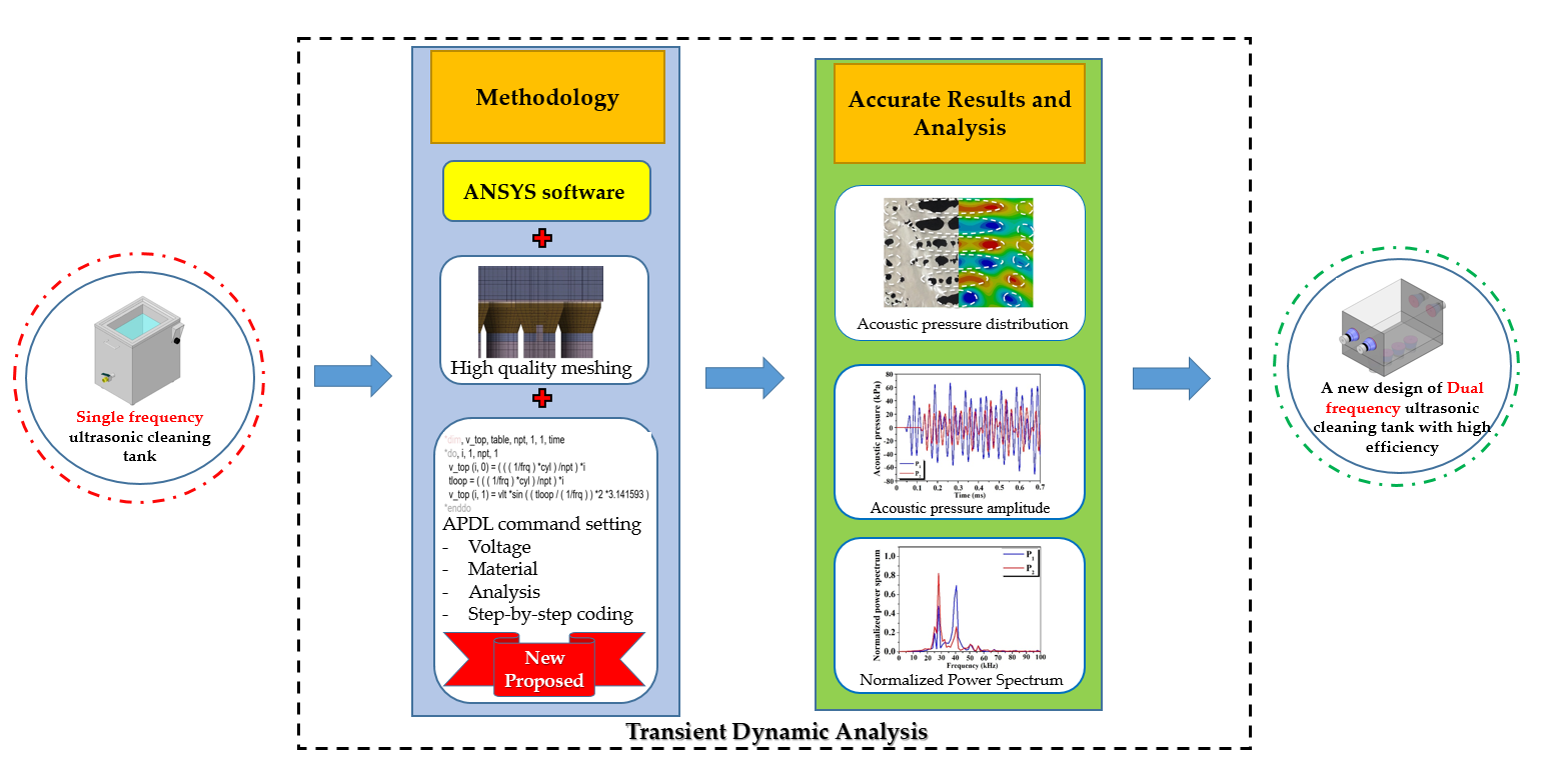
:At present, development of manufacturer’s ultrasonic cleaning tank (UCT) to match the requirements from consumers usually relies on computer simulation based on harmonic response analysis (HRA). However, this technique can only be used with single-frequency UCT. For dual frequency, the manufacturer used information from empirical experiment alongside trial-and-error methods to develop prototypes, resulting in the UCT that may not be fully efficient. Thus, lack of such a proper calculational method to develop the dual frequency UCT was a problem that greatly impacted the manufacturers and consumers. To resolve this problem, we proposed a new model of simulation using transient dynamics analysis (TDA) which was successfully applied to develop the prototype of dual frequency UCT, 400 W, 18 L in capacity, eight horn transducers, 28 and 40 kHz frequencies for manufacturing. The TDA can indicate the acoustic pressure at all positions inside the UCT in transient states from the start to the states ready for proper cleaning. The calculation also reveals the correlation between the positions of acoustic pressure and the placement positions of transducers and frequencies. In comparison with the HRA at 28 kHz UCT, this TDA yielded the results more accurately than the HRA simulation, comparing to the experiments. Furthermore, the TDA can also be applied to the multifrequency UCTs as well. In this article, the step-by-step development of methodology was reported. Finally, this simulation can lead to the successful design of the high-performance dual frequencies UCT for the manufacturers.

1. Introduction
Ultrasonic cleaning tank (UCT) is a piece of equipment used for cleaning tools or objects using the explosion (collapse) of a large amount of tiny bubbles within a medium. This phenomenon, so called cavitation effect, occurs when the acoustic pressure is rapidly changed by ultrasonic waves that ripple inside the medium. This effect can be applied into various situations, e.g., to improve the quality of raw materials in food factories [1,2,3], to deposit biomass or organisms to sediments [4,5], to eliminate marine biofouling [6,7,8], to clean medical or dental apparatus [9,10], and the most widely used situation is to clean tools, equipment, and other products in industries. The UCT is recommended as it can efficiently clean numerous objects at once, save cost, require a short period of time to clean, and can clean surfaces of small and complex shaped objects. These are the reasons why these UCT were the worthiest cleaning equipment of all methods [11,12,13]. In the case of large or simple shaped objects such as watches, glasses, gems, jewelry, etc., the single frequency UCT is sufficient for the task. However, if the object’s shape is complex, such as head gimbal assemblies, head stack assemblies, electronic cables, printed circuit boards, microchips, or other small electronic parts, the single frequency UCT which is commonly used may not be sufficient. This is why the dual frequency UCT was required. In single frequency UCT, even though they were thoughtfully designed, standing waves and stable cavitation within the tank inevitably occurred [14]. This caused objects to be inefficiently cleaned. From previous research, we discovered that the dual frequency UCT helped reduce standing waves and stable cavitation. This caused better transient cavitation and thus generated various sizes of bubbles, accelerating the bubbles’ collapsing rates, and intensifying the acoustic pressure within the bubbles [15,16,17,18,19,20,21,22] which benefited the cleaning process of small and complex shaped objects. Therefore, advanced factories that require these objects to be exceptionally clean widely used dual or multifrequency UCTs [1,3,14,15,16,17,18,19,20,21,22].
In the past, the development of computer simulations based on finite element method (FEM) was used to improve sonoreactors [23,24,25], ultrasonic transducers [26], and UCT [27] to help create the cavitation effect to the highest level [27]. Furthermore, our recent work cooperating with a manufacturer to develop a 28 kHz UCT showed that using the harmonic response analysis (HRA) in FEM can be credible, and suitable to be applied and actually used commercially [28,29,30,31]. However, HRA could only be used for the single frequency UCT and was not enough for the further recent demand. Therefore, the challenge for this research was finding a method to develop a dual frequency UCT that could yield accurate results and could be practically used in the industries. From further research, it was indicated that transient dynamic analysis (TDA) was used to design multifrequency ultrasonic transducers [26], investigate the vibration that occurs in the ultrasonic dental scaler tip [10], and improve the piezoelectric micropump for fuel delivery system [32]. As the TDA were used to investigate the vibrations that occur from various conditions that differed in terms of time, it exhibits potential to be applied in the dual frequency UCT. Since the TDA has never been used in development of the UCT or calculation of the acoustic pressure before, the challenge of this research was that the authors must determine how to apply the TDA into the actual cleaning conditions in the industry. This will lead to develop the new version of the dual frequency UCT that yields the high efficiency and response to the users’ demands.
This article reports the research that was collaboratively conducted with the manufacturer. We used TDA to develop the original version of the single frequency UCT into the new dual frequency UCT from the start to the level that we could design the UCT which is appropriate for commercial production. The TDA in the ANSYS software was used to simulate the acoustic pressure in the original 28 kHz UCT and compared to the results from the HRA calculation and the previous experimental results. The TDA simulation was improved until we reached the result at such confidential level. After that, we designed and developed the dual frequency UCT (28 and 40 kHz) until we ended up with a suitable UCT model with the highest cleaning performance and also suitable for the commercial production. The highlights of this research are the methodology and the parameter settings that were optimized until the results were accurate and economic in terms of the computational time whereas the computational resource was limited.
2. Theoretical Background
2.1. Transient Dynamic Analysis (TDA)
TDA is the analysis of the results that occur from the load in terms of time. It can be used to solve various problems in physics and engineering, e.g., structure, heat, electricity, vibration, etc. For example, in structural problems, if we define force as the load, the results in terms of time may be deformation, stress, strain, total force, etc. [33]. In thermal and/or electrical problems, the load may be heat flux and/or electricity while the result in terms of time may be thermal stress, thermal strain, temperature, total heat, current density, etc. [34]. These two examples mentioned above stated the simple cases of TDA in physics. However, in recent development, the TDA has been optimized to be able to calculate more complicated and diverse problems. Nowadays, the TDA has been implemented in commercial software as one of the tools in “computer simulation”. For the UCT case, the important factor that must be calculated is the acoustic pressure which indicates the cleaning efficiency. This calculation is related to the field called Multiphysics. Presently, there is not yet a physics equation that can directly calculate or find an exact solution. However, according to the real cleaning process, the simulation tends to be more complicated. This gives rise to more complication in finding an answer. Therefore, in this research the TDA in the ANSYS software was chosen to solve the problem. The calculation method to figure the acoustic pressure can be explained with the FEM principles as follows. To explain the occurrence of the cavitation, most research used the acoustic wave equation to calculate the acoustic pressure which occurred in the UCT using (1) [35],
where p is the acoustic pressure (Pa) and c is the acoustic velocity (m/s).
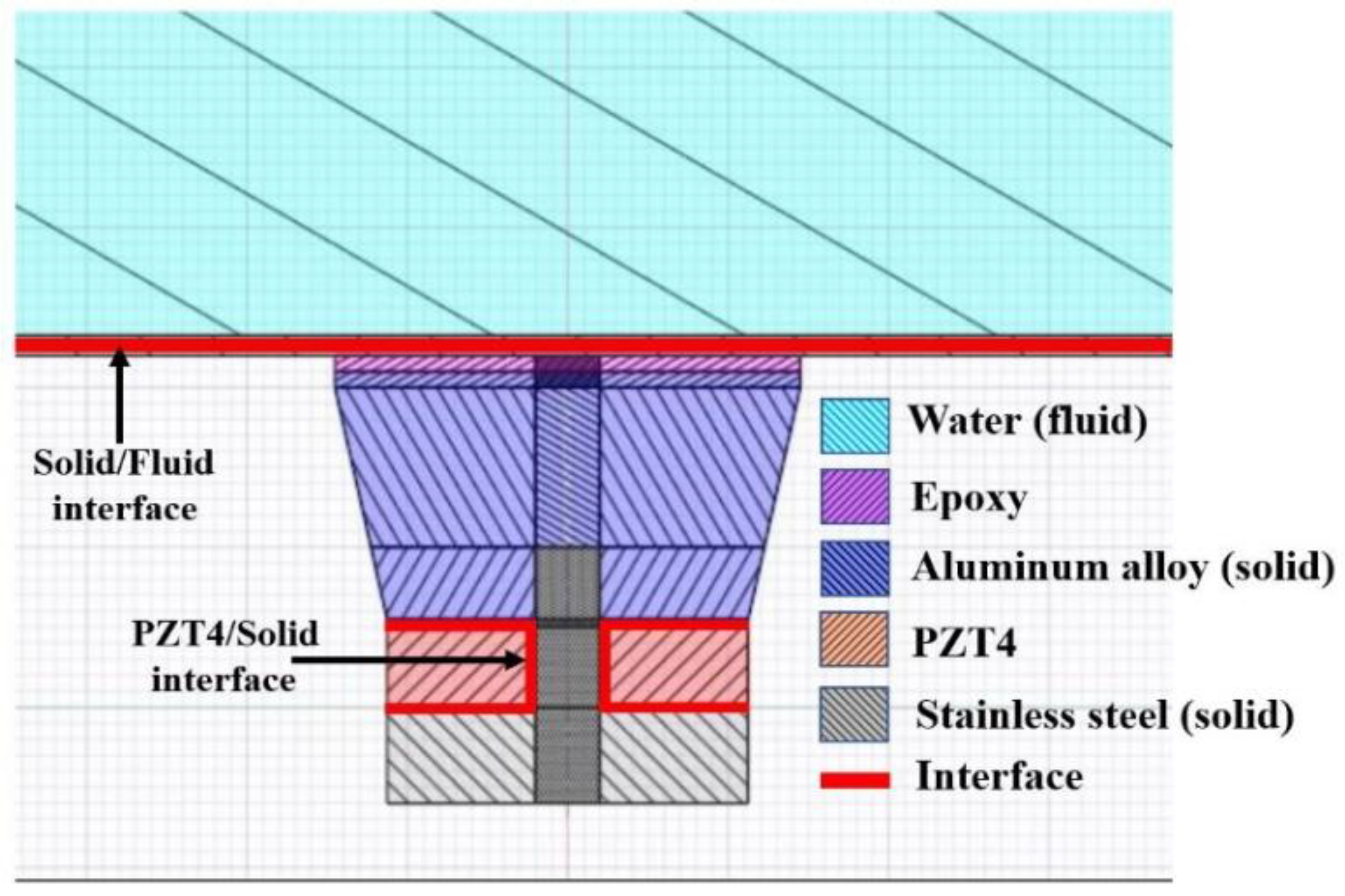
Once the lead zirconate titanate (PZT4) in the transducer received electric currents, it vibrated. This vibration caused the other parts of the tank to vibrate as well. The ultrasonic waves then transfer into the medium, in this case is water, eventually causing the cavitation effect. In the FEM point of view, we may consider that the UCT consists of three material domains and two interfaces. The material domains are the PZT4 which causes the vibration, the solid domain which is the hard metal parts such as the tank’s wall, front, and back mass which are made out of aluminum alloy and stainless steel, respectively, and lastly the fluid domain which is water or water solution mixed with surfactant to increase the cleaning efficiency. The interfaces are solid/fluid and PZT4/solid interfaces which are the connection areas between different material domains. Figure 1 shows material domains and interfaces for the FEM’s calculation.
In the PZT4 domain and PZT4/solid interface, the material’s vibration was caused by the coupling between a material’s mechanical and electrical responses. When PZT4 receives electric currents or voltages, vibrations in terms of {u} would occur and could be represented as in (2) [36] as
where [Muu] is coupling mass matrix (kg), [Cuu] is structural damping matrices (N s/m), [Cvv] is dielectric dissipation matrices, [Kuu] is structural stiffness matrices (N/m), [Kuv] is piezoelectric coupling element matrix, [Kvv] is dielectric permittivity matrices, F is mechanical load, Q is electrical load, {u} is nodal displacement vector (m), {} is nodal velocity vector (m/s), {ü} is nodal acceleration vector (m/s2), {V} is nodal voltage (V), {} and {} are the first and second derivatives of nodal voltage, respectively.
Afterwards, the {u} from (2) will be transferred to the solid domain, causing it to vibrate continuously. In this domain, {u} was calculated using (3) [37] as,
where [M] is mass matrix (kg), [C] is damping matrix (N s/m), and [K] is structural stiffness matrices (N/m).
The vibration of the solid domain caused ultrasonic waves which move towards the solid/fluid interface. The {u} of this region was calculated using (4) [35].
where [MS] is solid mass matrix (N s2/m), {ρf} is fluid density (kg/m3), [R]T is acoustic fluid boundary matrices (m3), [MF] is fluid mass matrix (N s2/Pa), [CS] is damping matrix (N s/m), [CF] is acoustic damping matrix (N s/Pa), [KS] is structural stiffness matrices (N/m), [KF] is acoustic fluid stiffness matrices (N/Pa), {fS} is structural load (N), {fF} is acoustic load (N), {p} is nodal acoustic pressure vector (Pa), {} and {} are the first and second derivatives of nodal acoustic pressure, respectively.
When ultrasonic waves moved towards the water domain, the acoustic pressure was calculated by solving the second order partial differential equation mentioned in (5). This equation came from the hypothesis that the propagation of the sound waves in the medium is linear without considering the shear stress and the density of the fixed medium. The TDA in the ANSYS software created an equation to calculate the acoustic pressure by using FEM. To calculate acoustic pressure, the fluid domain of (1) was changed to an acoustic domain using Galerkin’s procedure [35] by multiplying (1) with a testing function (w) and integrating all of the volume to get (5) from {u} which became {p}, defining the desired acoustic pressure [35] as,
When the material properties and boundary conditions are all determined, the software will numerically solve (1)–(5) to determine {p} before displaying the results in graphical colors for further analysis.
2.2. Harmonic Response Analysis (HRA)
Similar to TDA, but in addition, the HRA focuses on calculating the reaction of materials towards loads like sinusoidal waves in the steady state. Previously, this method was used to develop single frequency UCTs accurately [28,29,30,31,35]. The calculation of HRA by FEM principles can be explained briefly as the following statements.
HRA can be similarly calculated as the TDA but replaces (2)–(5) with specific equations that had been proven and used exclusively for the HRA case as in (6)–(9), respectively [35], as
Notice that from (6)–(9), all equations have ω, meaning that it can only be used for the single frequency type with no terms of time as it is calculated in the steady state. Oppositely, the TDA calculation in (2)–(5) had no terms of ω but composed with the derivatives of time. Later, the equations must be set to the time according to a value of the transducer’s frequency.
3. Methodology
In this section, we explain the research methodology step by step from the beginning to the end of software setting to get the accurate results in the optimized conditions to minimize the computational resource.
3.1. Ultrasonic Cleaning Tank (UCT)
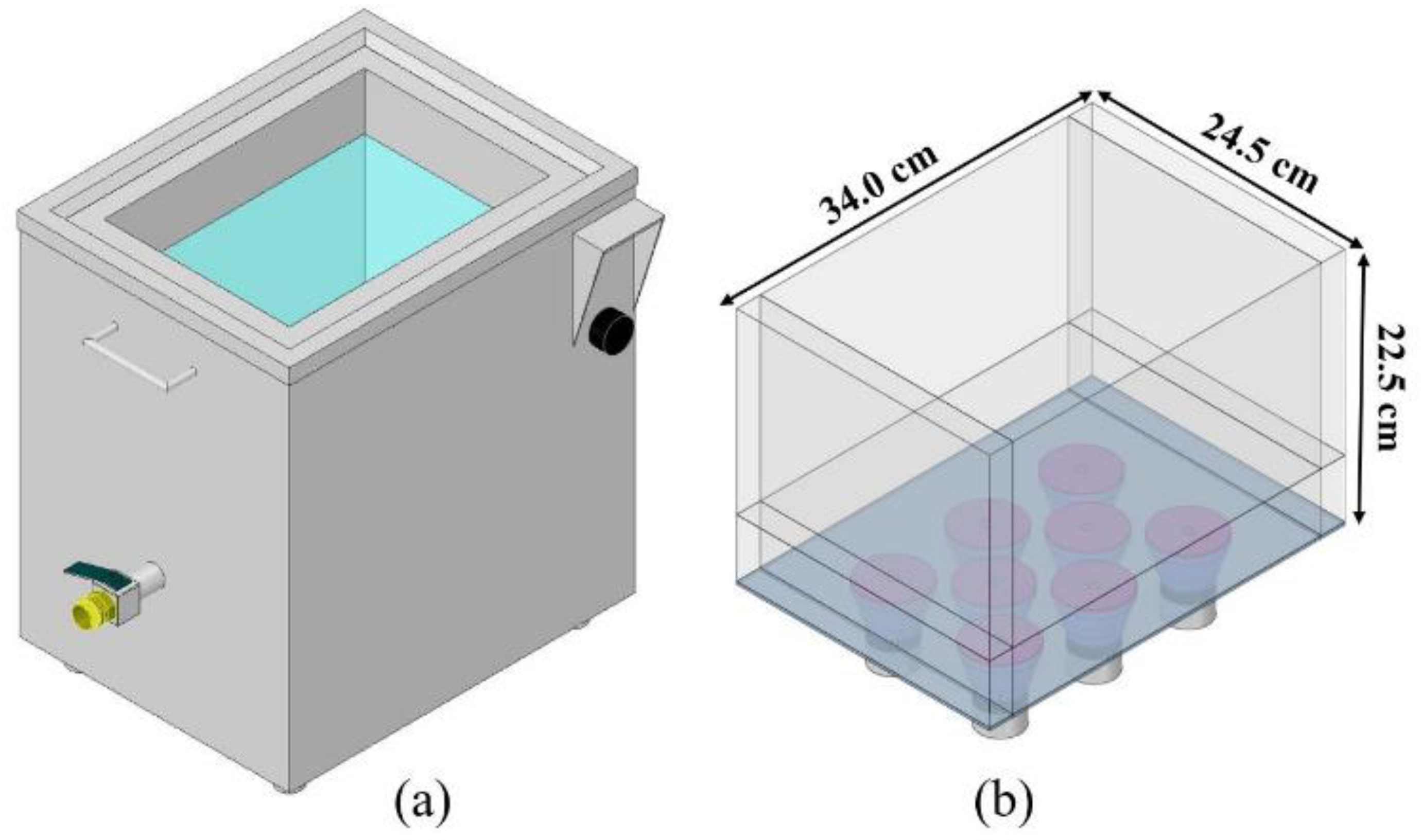
The manufacturer’s original UCT had a capacity of 18 L, eight horn transducers with frequency of 28 kHz, and 400 W in power. The walls and the lid were made of stainless steel. Figure 2 shows the CAD model of the UCT for (a) solid model that was used as the prototype to be developed. Once we filled the tank with water, the model was simplified and any irrelevant parts were removed as shown in Figure 2b. This model used water as the cleaning fluid. The transducers at the bottom had front mass made from aluminum alloy and back mass made from stainless steel. The walls and base made of stainless steel contained the water and acted as the main structure (see Figure 1 for the details). When the PZT4 received electric current or voltage, it would vibrate at a frequency of 28 kHz, generating an ultrasonic wave that transfers through the different parts and creating acoustic pressure in the water. The aim of the development is to improve this UCT model into the dual frequency model with frequencies of 28 and 40 kHz.
3.2. Mesh Model
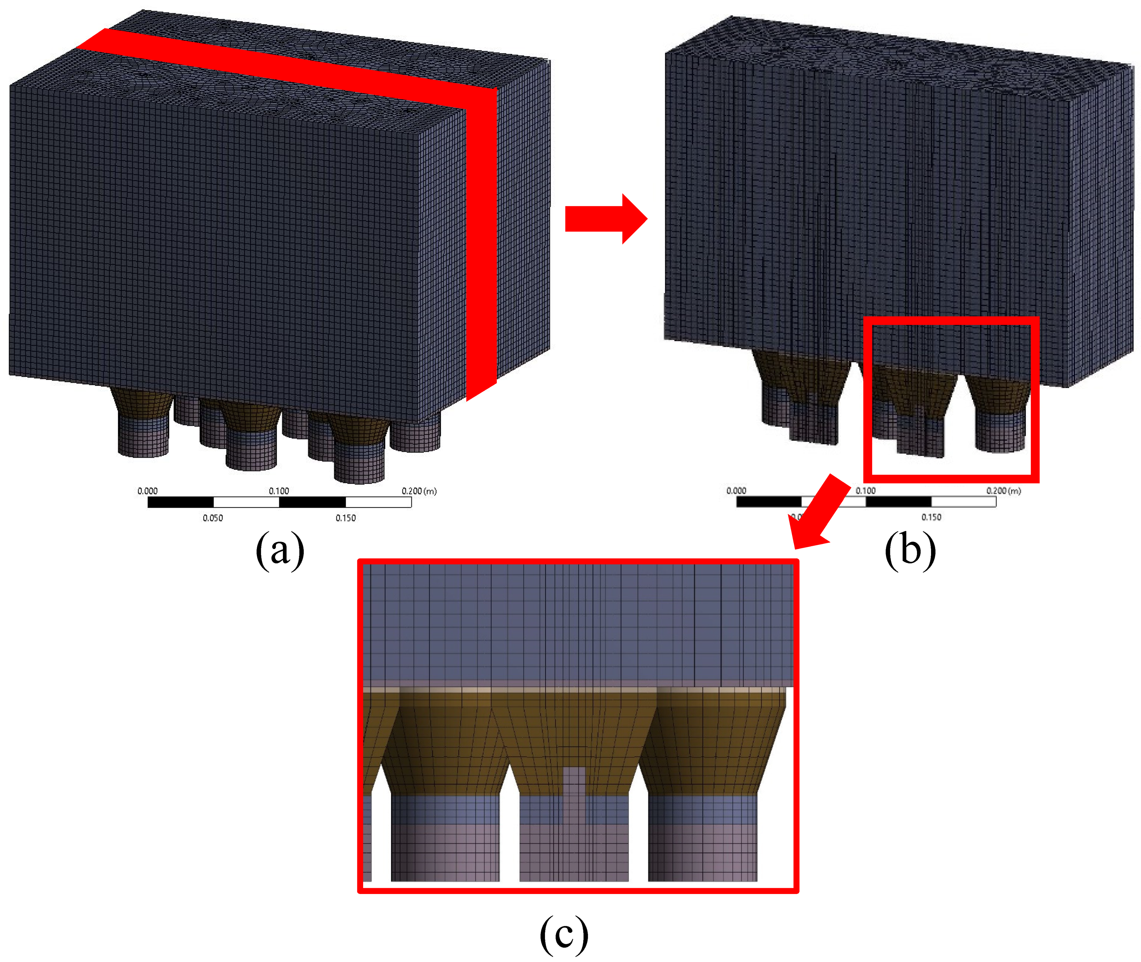
The TDA simulation results are sensitive to the quantity and quality of the mesh. If the quantity of the mesh is not sufficiently high or its quality is lower than expected, the result would be incorrect. In creating mesh for acoustic research, it is highly recommended to create mesh with at least six elements per wavelength to be able to capture any physical phenomena that occur in one of the longest wavelengths [35]. This was the strict criteria that we must always aware of. According to these criteria, we created the mesh with 10 elements per wavelength so it could cover the simulation for 40 kHz and was suitable for the limited computational resources. Once the CAD model in Figure 2b was taken as a prototype, we created the mesh model as in Figure 3. The mesh model was created with all hexahedrons, totaling 176,477 elements and 740,241 nodes. The average skewness was 0.35 and the maximum skewness was 0.8. Figure 3 shows (a) an overall image of the mesh, (b) a vertical cross section of the mesh, and (c) the mesh around the transducers as shown in (b). Conformal mesh was assigned to the interface areas. Notice that the mesh we created was highly detailed in quality to support the simulation of the TDA up to the frequency of 40 kHz. Creating the mesh model is vital. In prior calculations, the mesh was created with lesser elements of tetrahedrons or hexahedrons. After the mesh analysis, it was found that the results were not as accurate as the mesh in Figure 3. Furthermore, if the frequency is set to be higher (although the UCT is in the same size) it is highly recommended to necessarily increase the mesh quantity due to the strict rule as mentioned above.
3.3. Software Setting
The default setting of the TDA in the ANSYS software would not be able to calculate the acoustic pressure directly. It was therefore necessary to update the software with an additional package named ACT×2020R1 before it could be used [35,36]. This may cause additional expenses for some users. In this research, we proposed an alternative process without having to upgrade the package. To calculate the acoustic pressure, we must write up the ANSYS parametric design language (APDL) command additionally in three parts; material property, boundary condition, and analysis. As for the material property, originally in the PZT4 domain, the mesh’s default settings were Solid186 which could only be used to calculate the stress, strain, or to find answers related to the structural problems. The APDL command must be amended to be Solid226 which could resolve the coupling problem between the structural and electrical calculation [34]. In PZT4, the APDL command was changed from isotropic material to anisotropic material using parameters as in Table 1. We must also write the input voltage to be able to generate ultrasonic waves as well. As for the water domain, the mesh’s original default setting was Solid186, the APDL command that was written would be modified the mesh type to Fluid220 which can be used to calculate the acoustic pressure mentioned in (5) and (9). Further necessary material’s properties were set as in Table 1. For the stainless steel and interfaces, the setting is similar to the aforementioned contents.
As for the analysis setting, the time step size (s) is 1/20f and the end time (s) is 30/f. Therefore, as f = 40 kHz given the time step size = 1.25 µs and an end time = 750 µs which covered when f = 28 kHz as well. This setting means that we must calculate 600 points with 20 iterations per point, to show the results between 0 and 750 µs. The shorter time step size and the longer the end time can cause the results of acoustic pressure to be clearer and easier for the analysis. All mentioned settings were sufficient to create the reliable result. Therefore, any other settings can be left as default in the software or for automatic setting. Details of the APDL command used to set material properties, boundary conditions, and analysis settings were displayed in APDL_description.pdf attached as the supplementary material. The computational resource used in this research are CPU: 18 cores Xeon (R) @ 2.30 GHz, RAM: DDR4 64 GB @ 1440 Hz and GPU: AMD Radeon 2 GB.
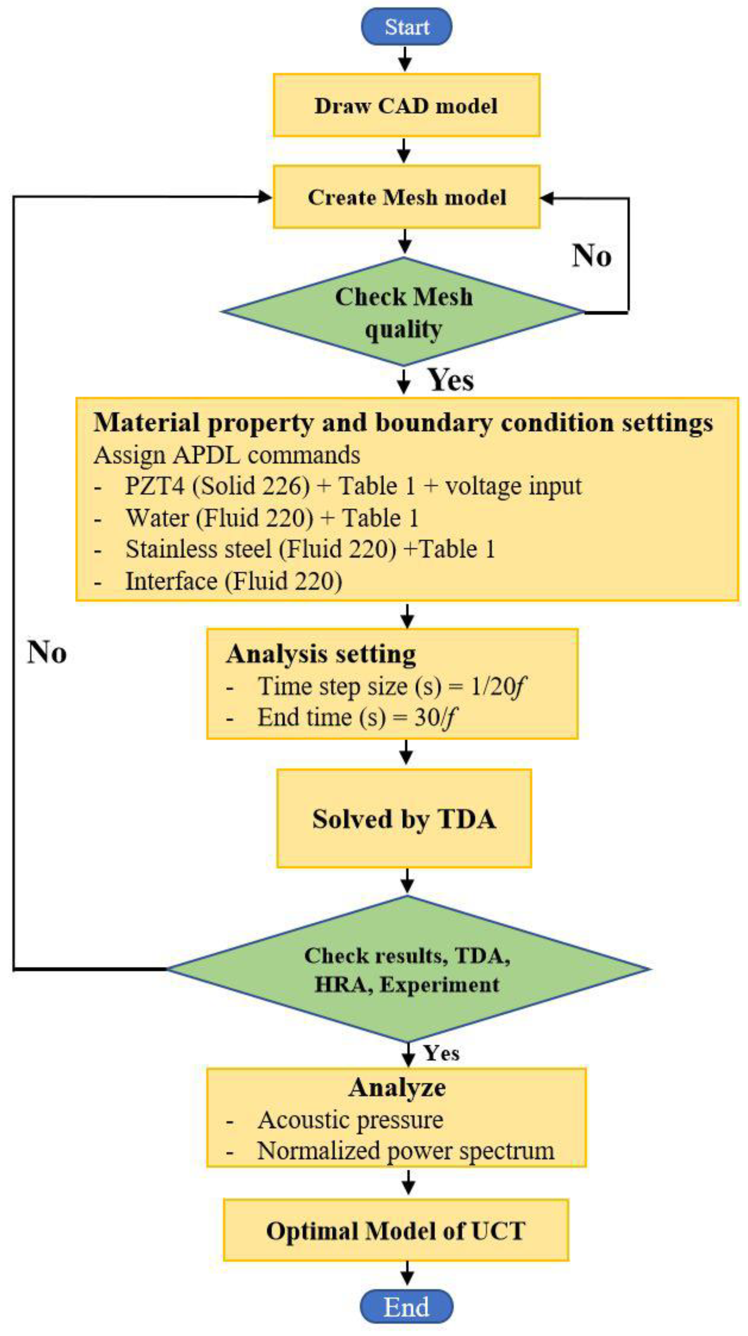
The most important part of the TDA simulation is creating such highly detailed mesh model as explained in Section 3.2 and setting the APDL command which makes the software calculate only the parts that are necessary, as mentioned in Section 3.3. All details of methodology were summarized and condensed into the flowchart in Figure 4.
4. Result and Discussion
4.1. Validation
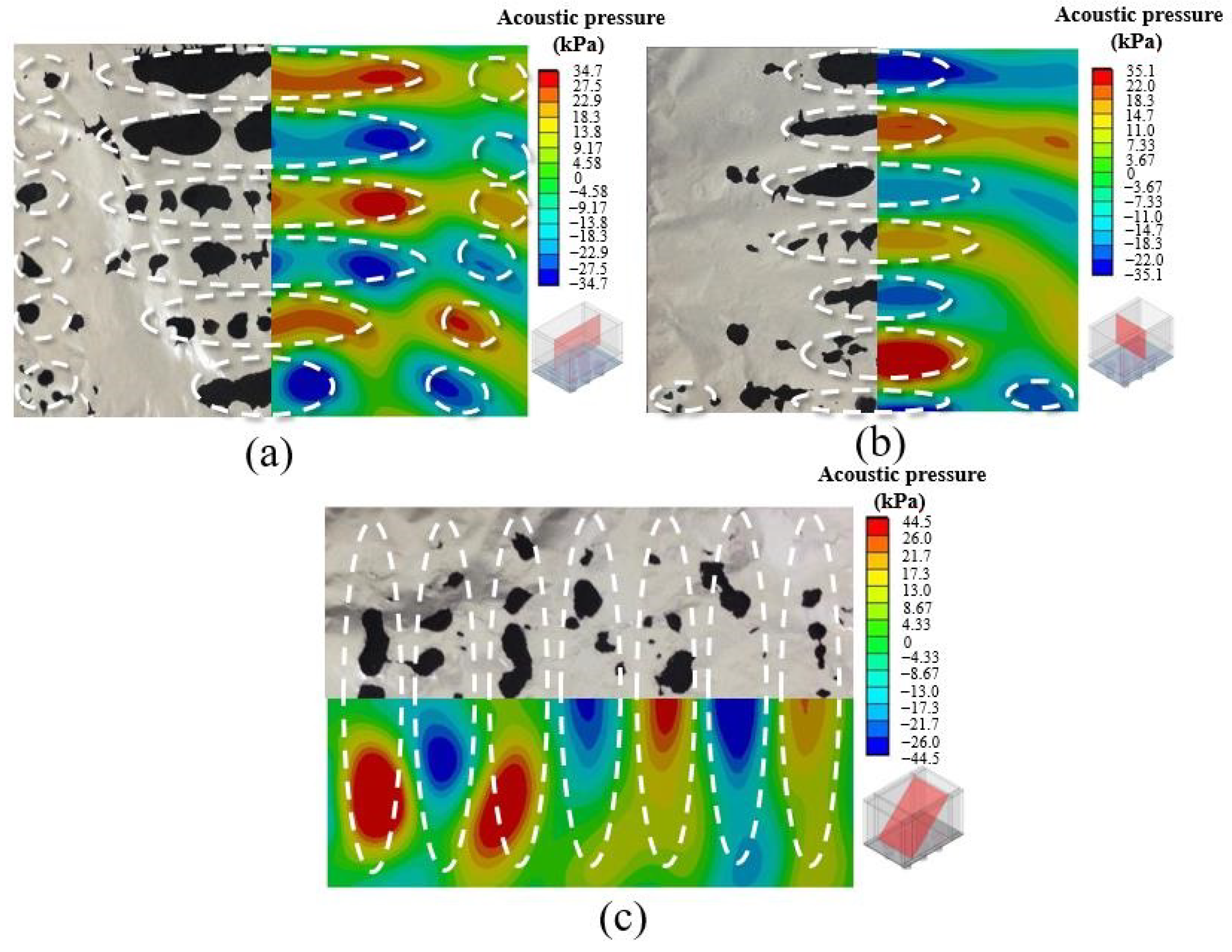
To test the reliability of the TDA before actual usage, in this research we compared results from the TDA to the actual experimental results from the foil corrosion test, mass loss, and power concentration which were retrieved from research [30] and compared them to the simulation using the HRA. The frequency and power were the variables. Conditions of the UCT simulation were; 28 kHz, 400 W in power, 18 L of capacity, eight horn transducers, and at temperature of 45 °C. These conditions were set as same as those in the previous research [30]. By using the TDA, we learned that there were specific distribution patterns which changed according to time and would repeat in a cycle between the maximum positive (+max) and the maximum negative (−max) values of acoustic pressure. When that patterns were compared to the foil corrosion test, the results are shown in Figure 5. Due to symmetry, we only displayed half of those symmetrical results. The small image show examples of the areas used in the comparison. We found that the distribution patterns were like the foil tear into three areas and were also close to the simulation results like the HRA reported in [28,30,31,38]. Therefore, we confirmed that tears in the foil could be predicted using the distribution of acoustic pressure from TDA. The difference between the −max value of acoustic pressure from the TDA in this research and the HRA in the previous research [30] for Figure 5a–c is less than 16.4%. We anticipated that the difference that occurred, apart from simulation method differences, was also caused by the mesh’s quality as well. We found that the mesh’s quality used in the HRA simulation of the previous research was lower than the one used in this research.
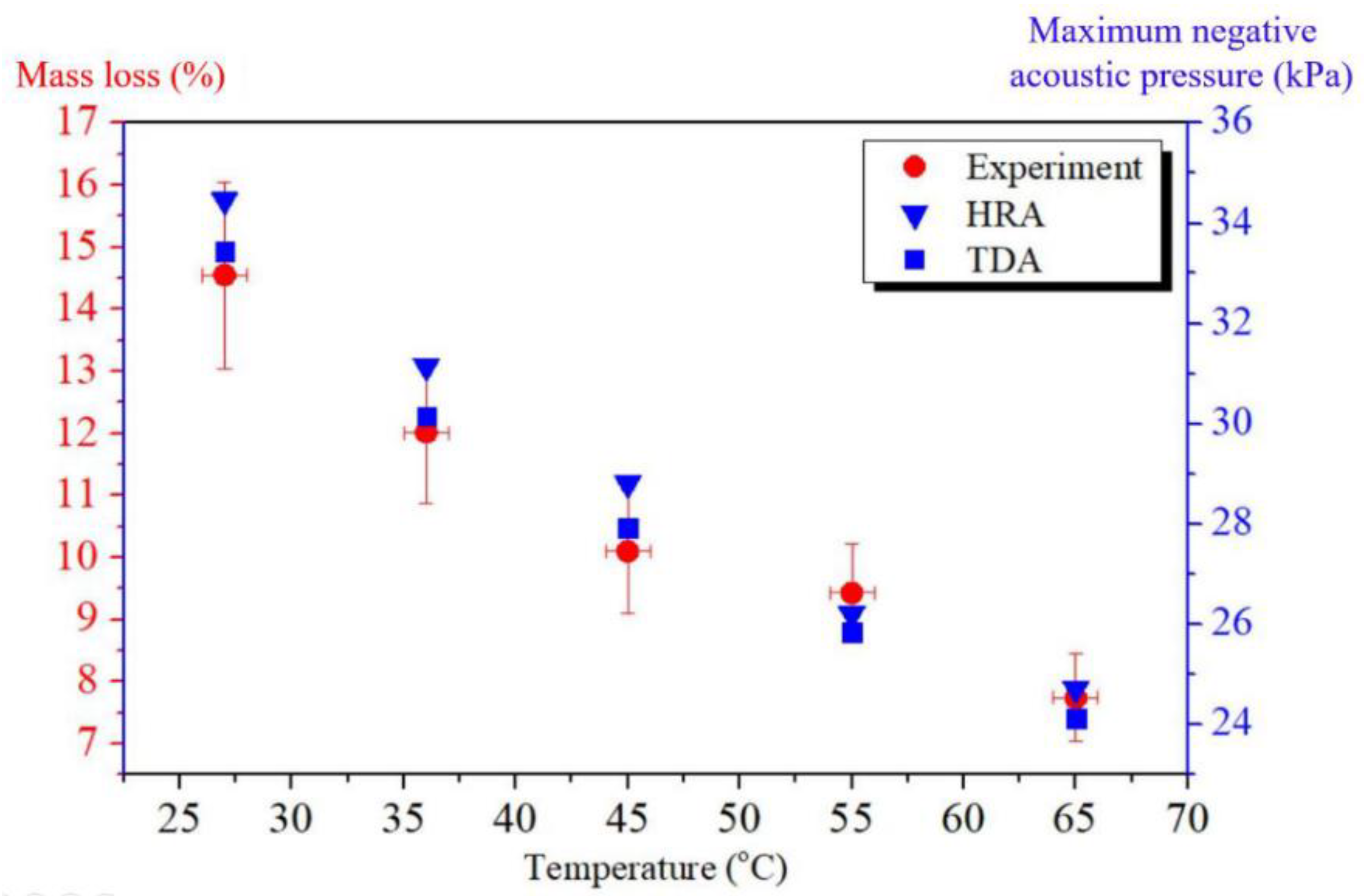
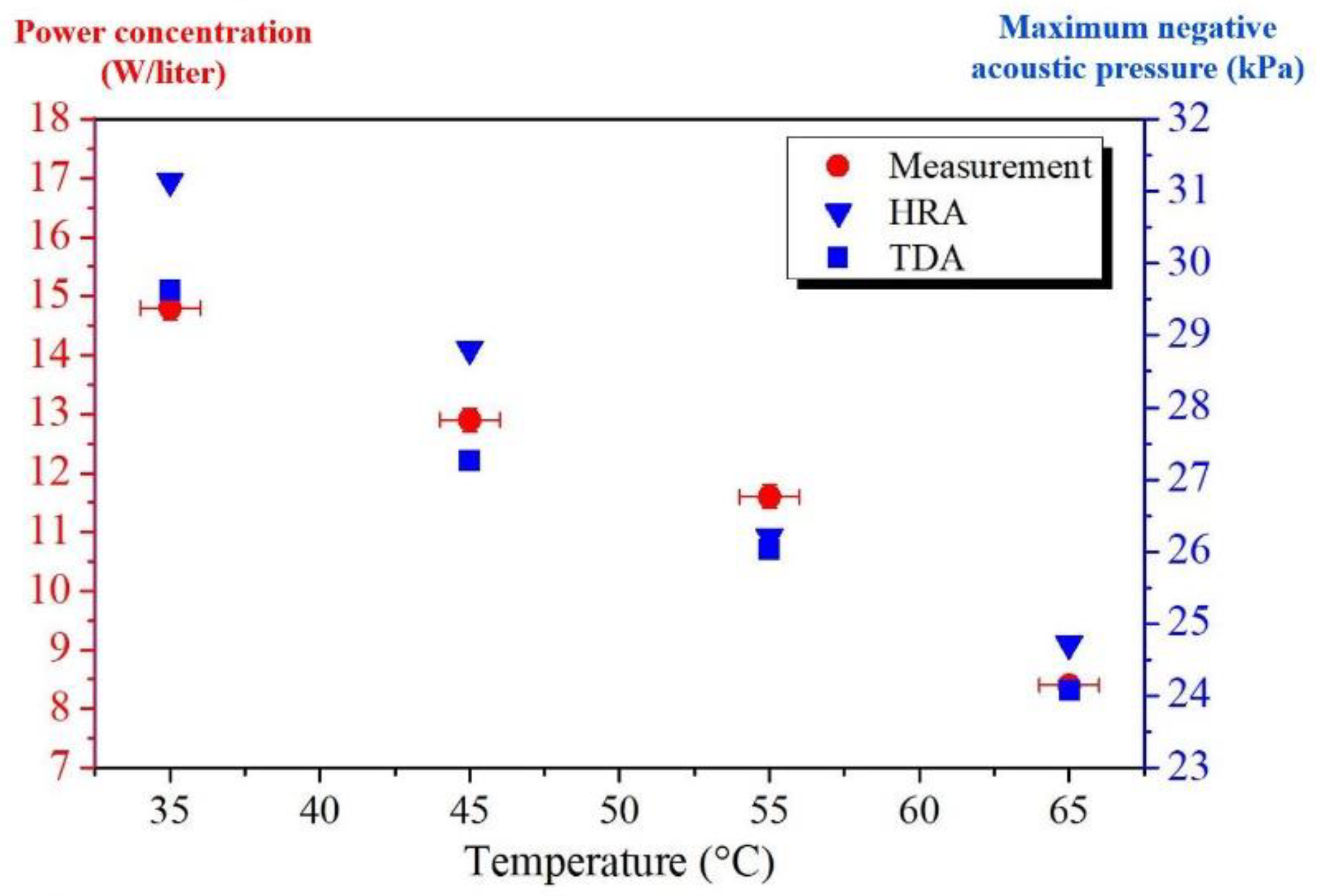
Figure 6 shows the acoustic pressure from the TDA, HRA, and experiment from mass loss of the foil from corrosion by cavitation for temperatures of 27–65 °C. The results of the foil’s mass loss were retrieved from research in [30], which was the test that weighed the corroded foil in Figure 5 using a highly sensitive digital scale with up to four digits. For the acoustic pressure gained from the HRA, in this image we repeat the simulation using the same settings reported in [30] but with the mesh model as in Figure 3. The result from the HRA and TDA will be compared and discussed in the discussion of Figure 5. From this figure, we found that when the temperature increased, the acoustic pressure from both TDA and HRA would decrease. This was greatly consistent with results of the mass loss. The acoustic pressures from the TDA were closer to the mass loss than the HRA ones. The difference of the results from the TDA and HRA were lower than 6.3% which decreased from 16.4% mentioned above as expected. Figure 7 shows the −max acoustic pressure from the TDA and HRA which used the same mesh model. Both simulation results were plotted compared to power concentration results measured by the NGL measurer model UPC 300 at a height of 17.5 cm from the bottom of the UCT with the temperatures ranging from 35 to 65 °C. Measurable results were retrieved from the research in [30]. We found that when temperatures rose, the −max acoustic pressure from both methods including the power concentration would decrease consistently. The TDA gave a −max acoustic pressure figure that was closer to the power concentration figure than the HRA. Figure 8 and show the acoustic pressure distributions from the TDA at the same area as in Figure 5a of 28 and 40 kHz UCTs, respectively. The power applied into the transducers was (a) 300, (b) 350, and (c) 400 W. We discovered that the increase in power also intensified the acoustic pressure while the distribution remained the same as reported in [28] which was simulated with the HRA in ANSYS software and [39] which was simulated with the Multiphysics in COMSOL software. These results indicated that when it comes to designing UCTs, both frequency and power of the transducer must be considered. After checking the correction of the TDA gained from Figure 5, Figure 6, Figure 7, Figure 8 and Figure 9, we were confident that the TDA method which we proposed could be used to simulate acoustic pressure in the UCT accurately and with more credibility than HRA.
4.2. Scheme to Develop Dual Frequency UCT
In this section, we shall discuss acoustic pressure simulation results in the dual frequency UCT model that we developed using the TDA. We also include analysis of the results which led to a model suitable enough for commercial production.
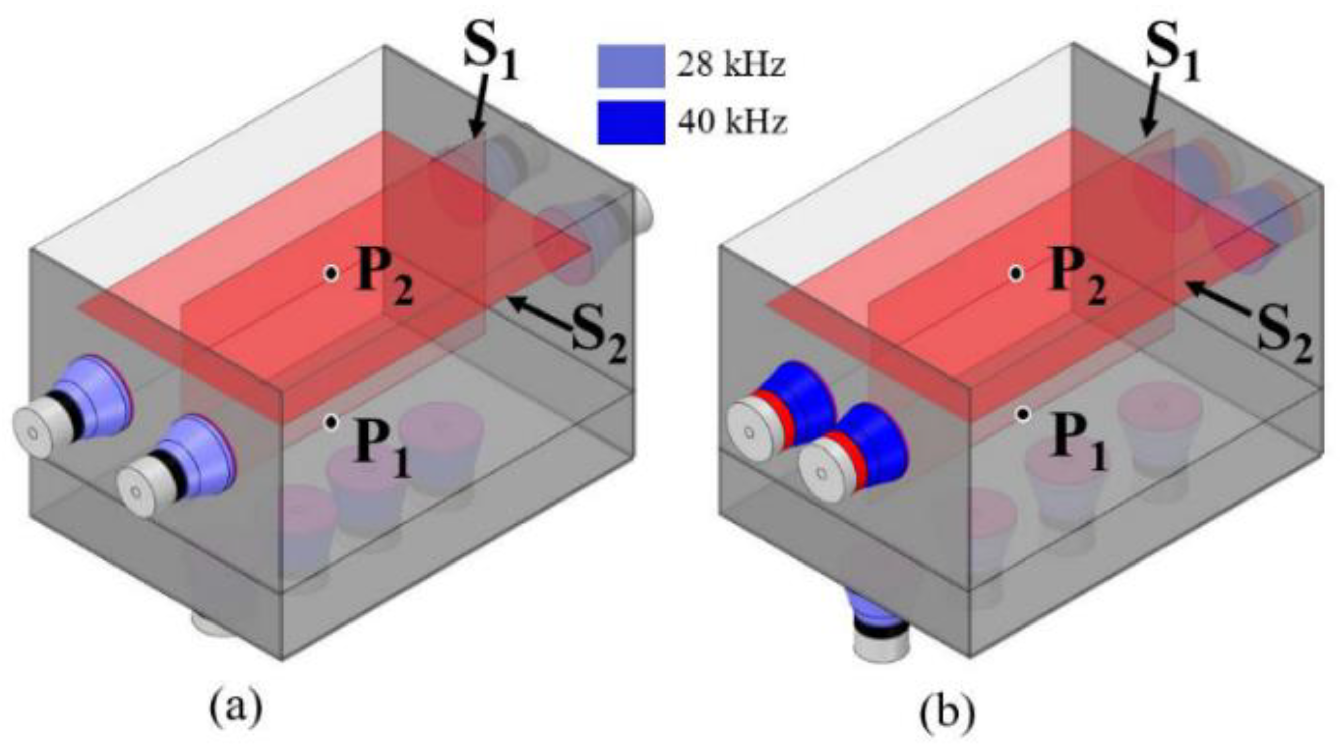
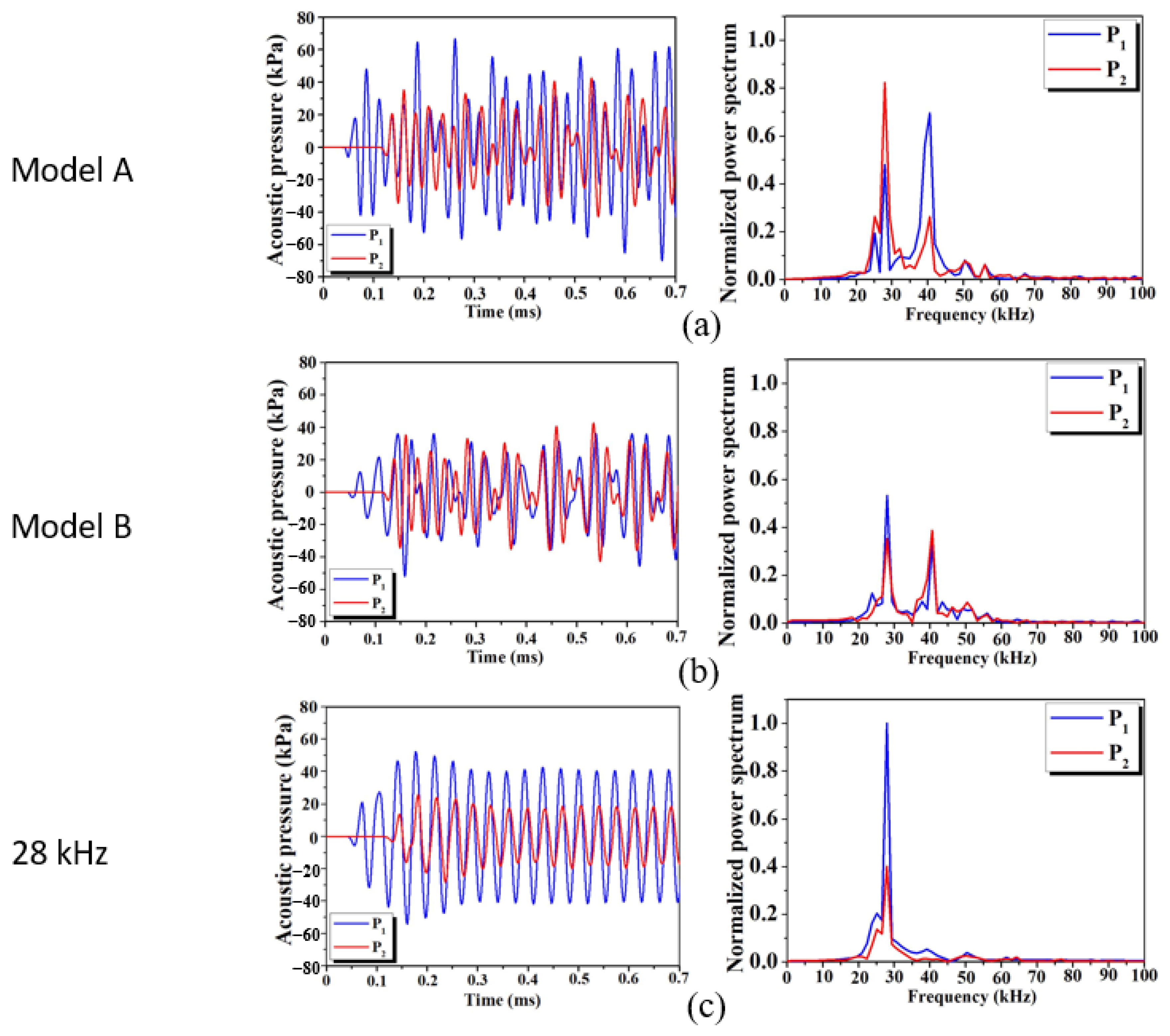
To save costs for the manufacturer, the original 28 kHz UCT model mentioned in Section 3.1 was chosen to be developed which was the same model reported in [30] and changed its frequency to be dual mode with 28 and 40 kHz transducers. The reasons why both frequencies were chosen are the production line is similar to the original UCT production and at these frequencies the models are popular for various jobs. It could be used to clean glasses, watches, gems, jewelry, small electronic parts, and others [31]. With support of information from the previous research [30], we designed this UCT with eight horn transducers. To boost cleaning efficiency, four transducers were placed linearly at the bottom of the tank, two transducers were placed horizontally on both sides of the tank. When the question about the optimal cleaning positions of 28 and 40 kHz transducers were raised, the TDA provided a satisfying answer to that. The simulation showed that there are two models of the most possible simulations as shown in Figure 10a,b named models A and B, respectively. The model A has two pieces of 28 kHz transducers on the sides which were placed horizontally and four pieces of 40 kHz transducers at the bottom of the tank, placed linearly. Oppositely, Figure 10b shows model B with four pieces of 28 kHz transducers at the bottom and two pieces of 40 kHz transducers on both sides of the tank. P1 and P2 were the central points which are 5.5 and 17.5 cm higher from the bottom of the tank, respectively. S1 is vertical surface, 5.5 cm higher from the bottom of the tank while S2 is horizontal surface, 17.5 cm higher from the bottom. We used the central points (P1 and P2) and mentioned surfaces (S1 and S2) as the reference points to analyze the acoustic pressure via the simulation. These positions all cover the places which the manufacturer recommended as they give rise to the highest cleaning efficiency. It was noted that both models share the same shape but have different dimensions and space between the transducers’ positions. We used the fact that the transducers were located at the antinode of the rectangular UCT given higher amplitude than other positions. Figure 11 on the left shows the acoustic pressure’s time domain while on the right shows the frequency domain of normalized power spectrum (NPS) which took acoustic pressure from the figure on the left and was calculated with fast Fourier transform (FFT) in MATLAB software for (a) model A, (b) model B, and (c) 28 kHz UCT at positions P1 (blue) and P2 (red). We simulated the acoustic pressure that occurred in the 28 kHz UCT in Figure 2 to compare the acoustic pressure from both dual and single frequency UCTs. Results of this simulation are displayed in Figure 11c. In addition, Table 2 shows the NPS values of models A, B, and 28 kHz at positions P1 and P2. In Figure 11a,b, both images on the left and right with positions P1 and P2 all clearly show ultrasonic waves merging which occurred from vibrations of the 28 and 40 kHz transducers. Small peaks on the right image occurred from acoustic pressure between ranges 0–0.05 ms which are not stable yet. In Figure 11a, from the left image, the ultrasonic waves arrived at P1 before P2 because P1 was closer to the transducers than P2. At P1, the NPS of 40 kHz transducer (NPS40 kHz) was approximately 0.70 which was higher than NPS of 28 kHz transducer (NPS28 kHz) that was 0.48. This was because in model A, P1 was placed nearer to the 40 kHz transducer than the 28 kHz transducer (see Figure 10). When we consider the P2, NPS28 kHz was as high as 0.82 while NPS40 kHz was only 0.26. The reason is the P2 was closer to the 28 kHz transducer than the 40 kHz one. For Figure 11b, the explanation is similar to above; placing the transducer in model B will change the NPS of both P1 and P2. At P1, NPS28 kHz and NPS40 kHz changed to 0.53 and 0.32, respectively, while at P2 NPS28 kHz and NPS40 kHz changed to 0.35 and 0.39, respectively. The image where ultrasonic waves merge in Figure 11a,b is similar to what was reported in Figure 2a by L. Ye, et al. [14] who studied the numerical increase of the cavitation effect caused by ultrasonic frequencies of 50 and 70 kHz. In Figure 11c, the left image clearly depicts that the acoustic pressure which occurred resulted from vibrations of only the 28 kHz transducer. There is no combination of two ultrasonic waves. This could once again confirm that the TDA yielded the accurate results. In this figure, the acoustic pressure at P1 is higher than P2 because position P1 is closer to the transducer than P2. The figure on the right also yielded relevant results; the NPS28 kHz had reached to the maximum value of 1.00 which was calculated by FFT using acoustic pressure of 51,630 Pa. The highest level at position P1 was used as a reference value for normalization. We normalized the acoustic pressure and calculated in MATLAB until we found the NPS at different positions as shown in Table 2. Apart from the information in Table 2, we also calculated the NPS at different points as well. Simulation results also are consistent with each other.
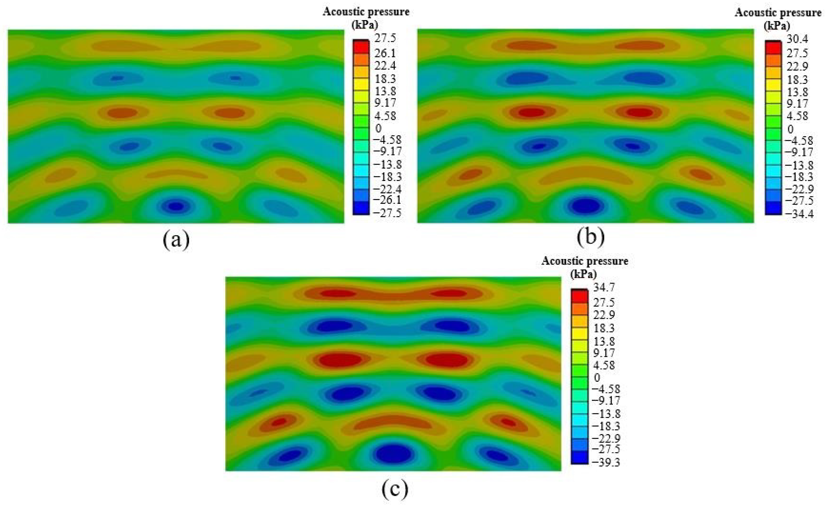
From the results in Figure 11a–c and Table 2, the TDA helped to confirm that the intensities of the NPS depended on the positions of the transducers and frequencies, which also were consistent with the report in [28,29,30,31]. Therefore, the model A is more suitable for the production than the model B as its NPS is higher in more places in the tank. However, it can be questioned whether the NPS could be used to confirm the UCT’s cleaning efficiency or not as there is no research that had analyzed the results in this routine. To confirm the reliability of the analysis using NPS, we simulated the acoustic pressure distribution in terms of time at S1 which was in the vertical position of Figure 12 for model A and Figure 13 for model B, respectively. Since the distribution shows the existence of ultrasonic waves, therefore in Figure 12 at 57.14 µs, the ultrasonic waves from the 28 kHz transducers came from both sides. Consequently, at 87.50 µs waves from the 40 kHz transducers below start to travel to S1 then the waves from both sides start to merge. At 104.46–213.39 µs the merged waves start to clearly form the distribution pattern. At 681.25 µs, +max acoustic pressure occurred, and at 698.20 µs, −max acoustic pressure occurred. After this period, the acoustic pressure may slightly change but would not exceed the +max and −max values. We may say that the distribution pattern of this period is the most suitable for cleaning as once reported in [28,29,30,31]. This may avoid the standing waves and stable cavitation that may decrease cleaning efficacy. Figure 13 shows the merging of ultrasonic waves from both frequencies in S1 for the model B. Similar to the previous figure, the −max and +max values of acoustic pressure occurred during 643.75 and 656.25 µs, respectively with different distribution patterns from Figure 12. Once we compared the distribution of the +max and −max values between model A in Figure 12 and model B in Figure 13, we discovered that model A gave the higher acoustic pressure level and had better distribution throughout the space of the tank than model B. From all of these reasons, we are confident that model A is better than model B. The animations supported the discussion in Figure 12 and Figure 13 are ModelA_S1.mp4 and ModelB_S1.mp4 attached in the supplementary material.
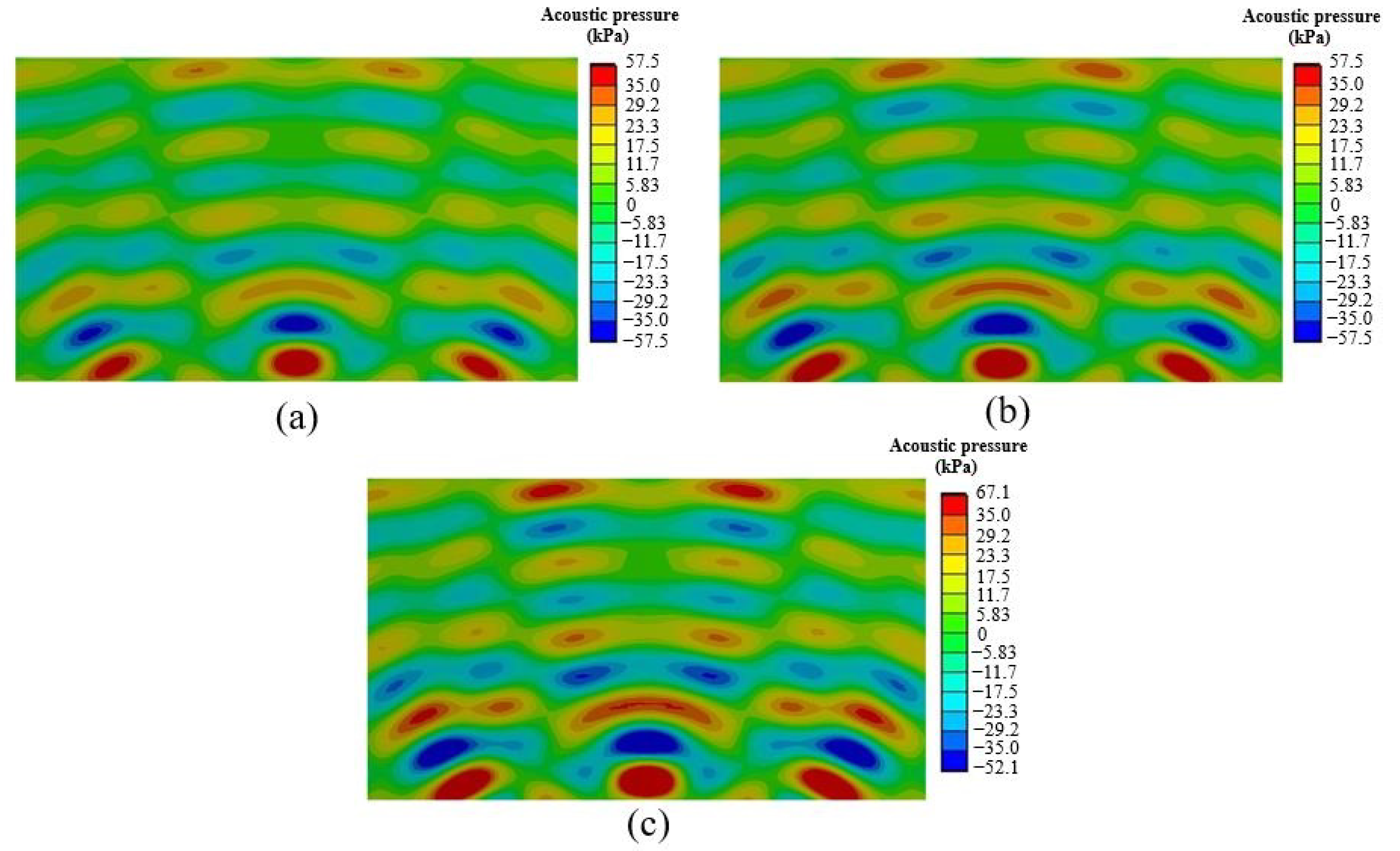
For further investigation, Figure 14 shows the acoustic pressure distributions in S2 during the time when −max and +max values occurred for (a) model A and (b) model B. The red and blue parts represent positive and negative values of acoustic pressure which had values higher than 25 kPa. We found that these acoustic pressure levels give rise to power concentration values of 9–10 W/liter [30] which is sufficient for cleaning electronic parts, gems, and jewelry in factories. Therefore, these criteria were set for considering the UCT’s cleaning performance. From the figure, it is noticeable that during the 0–750 µs range, model A gave −max and +max values of acoustic pressure at 608.93 and 697.32 µs, respectively. Meanwhile, model B did so at 521.43 and 545.54 µs, respectively. When Figure 14a,b was compared, we found that in model A, apart from giving such higher −max and +min values of acoustic pressure, it also had wider area (red and blue) which is more suitable for cleaning than model B. From this, it would be easier to design a jig or a handle to hold the object. It would also be able to clean objects better as well. We also found that for all vertical surfaces in UCT such as S1 and all horizontal areas such as S2, the −max or +min values would occur simultaneously. This matter leads to the fact that in vertical and horizontal arrangements, the −max or +min values of acoustic pressure would not occur at the same time. This result could be used to analyze and design a jig for holding the object that will be cleaned. After considering all results from Figure 11, Figure 12, Figure 13 and Figure 14, we found that they were consistent. This indicated that model A was more suitable as a model for the commercial production rather than model B. It also confirmed that the NPS could reasonably signify the UCT’s cleaning performance. We also used the TDA to simulate the acoustic pressure for the simple tanks with three pieces of 28, 40, and 60 kHz transducers. The simulation found that it worked fine as well but is not reported in this article due to the limitation of space. Still, it helped to confirm that the TDA could be applied to multifrequency tank designs. Higher ultrasonic frequencies produce smaller cavitation bubbles than lower frequencies; therefore, the UCTs with 28 and 40 kHz produce the cavitation bubble radius during 7–16 μm [40].
As mentioned in Section 3.3, the HRA and the TDA could be simulated with the ANSYS software by upgrading it with an additional package called ACT×2020R1 [35,36]. In this upgrade, the authors found that the software could give similar answers to what we did in this research but required more calculations and other settings. The added time was caused by the updated software having to calculate other figures that were irrelevant which was a waste of computational resource. With the computational resource that we had under the same circumstances, the time of the HRA used to calculate was approximately 30 min while the TDA used 8 h. Using the TDA with the additional package, it required 3–7 min longer than the method we used in this article (no additional package). The main part of this research was the APDL command which was used in the calculation and distributed by the authors in the supplementary materials for others who are interested. As for the pros and cons of the HRA and the TDA, it could be briefly said that the HRA could calculate acoustic pressure in shorter time, required no additional APDL command coding, used a humble amount of computational resource, and does not have the complicated setting. The HRA is therefore suitable for developing the single frequency UCT and gives very good calculational results. In contrast, the TDA was able to calculate acoustic pressure at the slower rate, requires additional APDL command coding, uses higher computational resource, has more complicated settings, but yields more accurate simulation than the HRA. It can also be used to develop both the single, dual, and multifrequency models. Now, both methods have been employed to develop UCTs in collaboration with the manufacturers.
As mentioned in Section 3.3, settings of the mesh size, time step size, and end time depend on the highest frequency. The higher of the frequency, the more computational resource is required in order to get reliable results. It may be said that if the computational resource is not high enough then the TDA could not be the suitable option. Hence, having limited computational resource was the main problem if one would like to design and develop high capacity UCTs with more transducers, as well as multifrequency tanks, thus, a guideline of possibility was using computational fluid dynamics (CFD) to aid. As seen in the article, when using the HRA and the TDA, we had to create the simulation model and build the UTC’s mesh model for the entire system as in Figure 1, Figure 2 and Figure 3. In reality, the acoustic pressure in the water could be calculated by {u} from the vibration of the transducers. If we had information of {u} in terms of time (both values from actual experiment and/or from simulation) we could use {u} as the source in CFD right away, or as to say, paving a shortcut to the calculation at (3) for the TDA and (7) for the HRA. This technique allows the design of UCT to disregard the calculation of the transducer’s vibration. Therefore, the transducer’s simulation model will not be required. This procedure also would lessen the computational resource. Developing a UCT with greater capacity with more transducers and higher frequency and into the multifrequency type using the CFD is, therefore, a new challenge for research. Certainly, if there is no limitation of the computational resource, the simulation using the TDA would not be a problem. However, as the limitation exists this research was performed as a stepping-stone for the others in the case of the higher frequency simulation in the future.
5. Conclusions
In this article, we successfully used the TDA in the computer simulation to develop the dual frequency UCTs for actual usage in the industry by cooperating with the manufacturer. Beforehand, the manufacturer’s development was limited to only the single frequency tank. The HRA was able to help to design and develop the UCT with high cleaning performance but it could not be used with dual or multifrequency UCTs. To be applicable in actual industrial settings, we boosted the numerical calculation capabilities of the TDA in the ANSYS software to be able to simulate acoustic pressure in UCT in the more accurate way. The high-quality mesh model was created, an APDL command was added in the software settings, and the time step calculation was set to be suitable for the limited computational resources. To validate the TDA’s reliability, it was deployed to simulate acoustic pressure in the UCT model that we had previously studied with experiments and the HRA simulation. Calculational results from the TDA, HRA, and actual experiments are highly consistent. When results from the TDA were compared to results from the HRA under the same conditions, we found that results from the TDA are more accurate. Therefore, the TDA we used was credible and could confidently simulate the acoustic pressure in the UCT. To develop the new dual frequency UCT which consisted of 28 and 40 kHz frequency transducers for manufacturing, we presented two models that possibly give rise to the best cleaning results. Both simulation models are exactly the same but only different at the transducer positions. By using the TDA to simulate acoustic pressure within both presented UCT models, the TDA showed the distribution in a transient state of all positions within the UCT which correlated with the placement and the transducer’s frequency. The results of acoustic pressure could be shown in time domain and used to calculate the NPS in frequency domain for analyzing and finding the suitable model. When these results were analyzed, we found that the two pieces of 28 kHz transducers on both sides and four pieces of 40 kHz transducers linearly placed at the bottom are the most suitable model. This setting provides the acoustic pressure with more intensity and dispersed evenly throughout the space of the tank than other models. We also found that the TDA could also be applied to multifrequency tanks and the NPS could be used to reasonably analyze its cleaning performance. The steps to use this TDA from the start to the finish were reported as the suitable UCT which the manufacturer could commercially benefit from.
Supplementary Materials
The following are available online at https://www.mdpi.com/2076-3417/11/2/699/s1, The APDL description and animation files used to support the finding of this research are included within the Supplementary Materials.
Author Contributions
Conceptualization, W.T. and J.T.; methodology, W.T. and J.T.; software, W.T.; validation, W.T. and J.T., formal analysis, J.T.; investigation, J.T.; writing—original draft preparation, W.T.; writing—review and editing, J.T.; project administration, J.T.; funding acquisition, J.T. All authors have read and agreed to the published version of the manuscript.
Funding
The fund was sponsored by Research and Researchers for Industry (RRI) under a grant number PHD61I0040.
Institutional Review Board Statement
Not applicable.
Informed Consent Statement
Not applicable.
Data Availability Statement
The additional figures and animations used to support the findings of this research are included within the supplementary materials.
Acknowledgments
This research was supported by Seagate Technology (Thailand) Ltd., Pasuda Supplies and Services Co. Ltd., College of Advanced Manufacturing Innovation, and King Mongkut’s Institute of Technology Ladkrabang. The fund was sponsored by Research and Researchers for Industry (RRI) under a grant number PHD61I0040. The authors also thank W. Busayaporn, Synchrotron Light Research Institute (SLRI), for the useful and supportive discussion.
Conflicts of Interest
The authors declare that there are no conflicts of interest for this article.
Nomenclature
| i, j | 1, 2, 3 correspond to the components of x, y, and z, respectively |
| {},{} | 1st and 2nd derivatives of nodal acoustic pressure vector. |
| {}, {} | 1st and 2nd derivatives of nodal voltage vector. |
| [CF] | acoustic damping matrix (N s/Pa) |
| [KF] | acoustic fluid stiffness matrices (N/Pa) |
| {fF} | acoustic load (N) |
| p | acoustic pressure (Pa) |
| [R]T | acoustic fluid boundary matrices (m3) |
| c | acoustic velocity (m/s) |
| ω | angular frequency (rad/s) |
| [Muu] | coupling mass matrix (kg) |
| [C] | damping matrix (N s/m) |
| [Cvv] | dielectric dissipation matrices |
| [Kvv] | dielectric permittivity matrices |
| {Q} | electrical load |
| {ρf} | fluid density (kg/m3) |
| [MF] | fluid mass matrix (N s2/Pa) |
| HRA | harmonic response analysis |
| [M] | mass matrix (kg) |
| +max | maximum positive acoustic pressure (Pa) |
| −max | maximum negative acoustic pressure (Pa) |
| {p} | nodal acoustic pressure vector (Pa) |
| {u} | nodal displacement vector (m) |
| {V} | nodal voltage vector (V) |
| NPS | normalized power spectrum |
| [Kuv] | piezoelectric coupling element matrix |
| [MS] | solid mass matrix (N s2/m) |
| [CS], [Cuu] | structural damping matrices (N s/m) |
| {F}, {fS} | structural load (N) |
| [K], [Kuu], [KS] | structural stiffness matrices (N/m) |
| f | transducer frequency (Hz) |
| TDA | transient dynamic analysis |
| t | time (s) |
| UCT | ultrasonic cleaning tank |
References
- Zheng, J.; Li, Q.; Hu, A.; Yang, L.; Lu, J.; Zhang, X.; Lin, Q. Dual-frequency ultrasound effect on structure and properties of sweet potato starch. Starch Stärke 2013, 65, 621–627. [Google Scholar] [CrossRef]
- Zhu, F.; Li, H. Modification of quinoa flour functionality using ultrasound. Ultrason. Sonochem. 2019, 52, 305–310. [Google Scholar] [CrossRef] [PubMed]
- Zhang, H.; Chen, G.; Liu, M.; Mei, X.; Yu, Q.; Kan, J. Effects of multi-frequency ultrasound on physicochemical properties, structural characteristics of gluten protein and the quality of noodle. Ultrason. Sonochem. 2020, 67, 105135. [Google Scholar] [CrossRef] [PubMed]
- Rodriguez-Molares, A.; Dickson, S.; Hobson, P.; Howard, C.; Zander, A.; Burch, M. Quantification of the ultrasound induced sedimentation of Microcystis aeruginosa. Ultrason. Sonochem. 2014, 21, 1299–1304. [Google Scholar] [CrossRef] [PubMed]
- Leclercq, D.J.J.; Howard, C.; Hobson, P.; Dickson, S.; Zander, A.C.; Burch, M. Controlling cyanobacteria with ultrasound. In Proceedings of the INTERNOISE 2014—43rd International Congress on Noise Control Engineering: Improving the World Through Noise Control, Melbourne, Australia, 16–19 November 2014. [Google Scholar]
- Salta, M.; Goodes, L.R.; Maas, B.J.; Dennington, S.P.; Secker, T.J.; Leighton, T.G. Bubbles versus biofilms: A novel method for the removal of marine biofilms attached on antifouling coatings using an ultrasonically activated water stream. Surf. Topogr. Metrol. Prop. 2016, 4, 034009. [Google Scholar] [CrossRef]
- Lais, H.; Lowe, P.S.; Gan, T.H.; Wrobel, L.C. Numerical modelling of acoustic pressure fields to optimize the ultrasonic cleaning technique for cylinders. Ultrason. Sonochem. 2018, 45, 7–16. [Google Scholar] [CrossRef]
- Lais, H.; Lowe, P.S.; Gan, T.H.; Wrobel, L.C. Numerical investigation of design parameters for optimization of the in-situ ultrasonic fouling removal technique for pipelines. Ultrason. Sonochem. 2019, 56, 94–104. [Google Scholar] [CrossRef]
- Felver, B.; King, D.C.; Lea, S.C.; Price, G.J.; Damien Walmsley, A. Cavitation occurrence around ultrasonic dental scalers. Ultrason. Sonochem. 2009, 16, 692–697. [Google Scholar] [CrossRef] [Green Version]
- Manmi, K.M.A.; Wu, W.B.; Vyas, N.; Smith, W.R.; Wang, Q.X.; Walmsley, A.D. Numerical investigation of cavitation generated by an ultrasonic dental scaler tip vibrating in a compressible liquid. Ultrason. Sonochem. 2020, 63, 104963. [Google Scholar] [CrossRef]
- Vetrimurugan, R. Optimization of Hard Disk Drive Heads Cleaning by Using Ultrasonics and Prevention of Its Damage. Apcbee Procedia 2012, 3, 222–230. [Google Scholar] [CrossRef] [Green Version]
- Vetrimurugan; Goodson, J.; Lim, T. Ultrasonic and megasonic cleaning to remove nano-dimensional contaminants from various disk drive components. Int. J. Innov. Res. Sci. Eng. Technol. 2013, 2, 5971–5977. [Google Scholar]
- Mason, T.J. Ultrasonic cleaning: An historical perspective. Ultrason. Sonochem. 2016, 29, 519–523. [Google Scholar] [CrossRef] [PubMed]
- Ye, L.; Zhu, X.; Liu, Y. Numerical study on dual-frequency ultrasonic enhancing cavitation effect based on bubble dynamic evolution. Ultrason. Sonochem. 2019, 59, 104744. [Google Scholar] [CrossRef] [PubMed]
- Yasui, K. A new formulation of bubble dynamics for sonoluminescence. Electron. Commun. Jpn. (Part II Electron.) 1998, 81, 39–45. [Google Scholar] [CrossRef]
- Lee, M.; Oh, J. Synergistic effect of hydrogen peroxide production and sonochemiluminescence under dual frequency ultrasound irradiation. Ultrason. Sonochem. 2011, 18, 781–788. [Google Scholar] [CrossRef] [PubMed]
- Zhang, Y.; Du, X.; Xian, H.; Wu, Y. Instability of interfaces of gas bubbles in liquids under acoustic excitation with dual frequency. Ultrason. Sonochem. 2015, 23, 16–20. [Google Scholar] [CrossRef]
- Zhang, Y.; Zhang, Y.; Li, S. Combination and simultaneous resonances of gas bubbles oscillating in liquids under dual-frequency acoustic excitation. Ultrason. Sonochem. 2017, 35, 431–439. [Google Scholar] [CrossRef]
- Suo, D.; Govind, B.; Zhang, S.; Jing, Y. Numerical investigation of the inertial cavitation threshold under multi-frequency ultrasound. Ultrason. Sonochem. 2018, 41, 419–426. [Google Scholar] [CrossRef]
- Hegedus, F.; Klapcsik, K.; Lauterborn, W.; Parlitz, U.; Mettin, R. GPU accelerated study of a dual-frequency driven single bubble in a 6-dimensional parameter space: The active cavitation threshold. Ultrason. Sonochem. 2020, 67, 105067. [Google Scholar] [CrossRef]
- Lee, J.; Hallez, L.; Touyeras, F.; Ashokkumar, M.; Hihn, J.Y. Influence of frequency sweep on sonochemiluminescence and sonoluminescence. Ultrason. Sonochem. 2020, 64, 105047. [Google Scholar] [CrossRef]
- Moholkar, V.S.; Rekveld, S.; Warmoeskerken, M.M.C.G. Modeling of the acoustic pressure fields and the distribution of the cavitation phenomena in a dual frequency sonic processor. Ultrasonics 2000, 38, 666–670. [Google Scholar] [CrossRef]
- Tudela, I.; Saez, V.; Esclapez, M.D.; Diez-Garcia, M.I.; Bonete, P.; Gonzalez-Garcia, J. Simulation of the spatial distribution of the acoustic pressure in sonochemical reactors with numerical methods: A review. Ultrason. Sonochem. 2014, 21, 909–919. [Google Scholar] [CrossRef] [PubMed] [Green Version]
- Wei, Z.; Weavers, L.K. Combining COMSOL modeling with acoustic pressure maps to design sono-reactors. Ultrason. Sonochem. 2016, 31, 490–498. [Google Scholar] [CrossRef] [PubMed] [Green Version]
- Rashwan, S.S.; Dincer, I.; Mohany, A. Investigation of acoustic and geometric effects on the sonoreactor performance. Ultrason. Sonochem. 2020, 68, 105174. [Google Scholar] [CrossRef]
- Henneberg, J.; Gerlach, A.; Cebulla, H.; Marburg, S. The potential of stop band material in multi-frequency ultrasonic transducers. J. Sound Vib. 2019, 452, 132–146. [Google Scholar] [CrossRef]
- Perincek, S.; Uzgur, A.E.; Duran, K.; Dogan, A.; Korlu, A.E.; Bahtiyari, I.M. Design parameter investigation of industrial size ultrasound textile treatment bath. Ultrason. Sonochem. 2009, 16, 184–189. [Google Scholar] [CrossRef]
- Tangsopha, W.; Thongsri, J.; Busayaporn, W. Simulation of ultrasonic cleaning and ways to improve the efficiency. In Proceedings of the 2017 International Electrical Engineering Congress (iEECON), Pattaya, Thailand, 8–10 March 2017; pp. 1–4. [Google Scholar]
- Tangsopa, W.; Keawklan, T.; Kesngam, K.; Ngaochai, S.; Thongsri, J. Improved Design of Ultrasonic Cleaning Tank Using Harmonic Response Analysis in ANSYS. IOP Conf. Ser. Earth Environ. Sci. 2018, 159, 012042. [Google Scholar] [CrossRef]
- Tangsopa, W.; Thongsri, J. Development of an industrial ultrasonic cleaning tank based on harmonic response analysis. Ultrasonics 2019, 91, 68–76. [Google Scholar] [CrossRef]
- Tangsopa, W.; Thongsri, J. A Novel Ultrasonic Cleaning Tank Developed by Harmonic Response Analysis and Computational Fluid Dynamics. Metals 2020, 10, 335. [Google Scholar] [CrossRef] [Green Version]
- Zhang, T. Valveless Piezoelectric Micropump for Fuel Delivery in Direct Methanol Fuel Cell (DMFC) Devices; University of Pittsburgh: Pittsburgh, PA, USA, 2005. [Google Scholar]
- Boonkaew, P.; Thongsri, J. The optimum design of micro gripper for lifetime improvement based on fatigue analysis and six sigma analysis. Int. J. Appl. Eng. Res. 2017, 12, 10233–10241. [Google Scholar]
- Thongsri, J. Transient Thermal-Electric Simulation and Experiment of Heat Transfer in Welding Tip for Reflow Soldering Process. Math. Probl. Eng. 2018, 2018, 4539054. [Google Scholar] [CrossRef]
- Ansys Inc. Introduction to Acoustics; ANSYS Europe Ltd.: Canonsburg, PA, USA, 2017. [Google Scholar]
- Ansys Inc. Piezo and MEMS ACTx R180; ANSYS Europe Ltd.: Canonsburg, PA, USA, 2018. [Google Scholar]
- Ansys Inc. ANSYS 2020 R1. In ANSYS Mechanical APDL Theory Reference; ANSYS Europe Ltd.: Canonsburg, PA, USA, 2020. [Google Scholar]
- Niazi, S.; Hashemabadi, S.H.; Razi, M.M. CFD simulation of acoustic cavitation in a crude oil upgrading sonoreactor and prediction of collapse temperature and pressure of a cavitation bubble. Chem. Eng. Res. Des. 2014, 92, 166–173. [Google Scholar] [CrossRef]
- Li, F.; Ge, S.; Qin, S.; Hao, Q. Simulation of Ultrasonic Cleaning and Experimental Study of the Liquid Level Adjusting Method. In Proceedings of the Re-Engineering Manufacturing for Sustainability, Singapore, 17–19 April 2013; pp. 275–278. [Google Scholar]
- John, F. Ultrasonic Intensity Measurement Techniques. JASA 1965, 38, 817–823. [Google Scholar]
Figure 1.
Material domains and interfaces.

Figure 2.
A conventional ultrasonic cleaning tank (UCT): (a) CAD model and (b) simplified model.

Figure 3.
Mesh model (a) in overview, (b) in vertical cross section, and (c) around the transducers.
Figure 3.
Mesh model (a) in overview, (b) in vertical cross section, and (c) around the transducers.

Figure 4.
Flowchart of methodology.

Figure 5.
Acoustic pressure distribution from the TDA in some areas compared to the results from foil corrosion test. (a) lengthwise, (b) crosswise, and (c) oblique, along the bottom base.
Figure 5.
Acoustic pressure distribution from the TDA in some areas compared to the results from foil corrosion test. (a) lengthwise, (b) crosswise, and (c) oblique, along the bottom base.

Figure 6.
The maximum negative acoustic pressure from the TDA and the HRA compared to the mass loss from the foil corrosion test.
Figure 6.
The maximum negative acoustic pressure from the TDA and the HRA compared to the mass loss from the foil corrosion test.

Figure 7.
The maximum negative acoustic pressure from the TDA and the HRA compared to the power concentration from measurement.
Figure 7.
The maximum negative acoustic pressure from the TDA and the HRA compared to the power concentration from measurement.

Figure 8.
Acoustic pressure distribution from the TDA of 28 kHz UCT for transducer power of (a) 300, (b) 350, and (c) 400 W.
Figure 8.
Acoustic pressure distribution from the TDA of 28 kHz UCT for transducer power of (a) 300, (b) 350, and (c) 400 W.

Figure 9.
Acoustic pressure distribution from the TDA of 40 kHz UCT for transducer power of (a) 300, (b) 350, and (c) 400 W.
Figure 9.
Acoustic pressure distribution from the TDA of 40 kHz UCT for transducer power of (a) 300, (b) 350, and (c) 400 W.

Figure 10.
Most possible models for simulation: (a) model A and (b) model B.

Figure 11.
Acoustic pressure’s time domain (left) and normalized power spectrum’s frequency domain (right) for (a) model A, (b) model B, and (c) 28 kHz.
Figure 11.
Acoustic pressure’s time domain (left) and normalized power spectrum’s frequency domain (right) for (a) model A, (b) model B, and (c) 28 kHz.

Figure 12.
Acoustic pressure distribution in terms of time at S1 for model A.

Figure 13.
Acoustic pressure distribution in terms of time at S1 for model B.

Figure 14.
Acoustic pressure distribution in S2 during the time when the maximum negative (left) and positive (right) values occurred for (a) model A and (b) model B.
Figure 14.
Acoustic pressure distribution in S2 during the time when the maximum negative (left) and positive (right) values occurred for (a) model A and (b) model B.


Table 1.
Material properties [28].
Table 1.
Material properties [28].
| Domain | Type | Value |
|---|---|---|
| Water (45 °C) | Water density | 990.15 kg/m3 |
| Acoustic velocity | 1533.5 m/s | |
| Dynamic viscosity | 5.7977 × 10⁻⁴ kg/ms | |
| Aluminum alloy | Density | 2770 kg/m3 |
| Young’s modulus | 7.1 × 10¹⁰ Pa | |
| Poisson’s ratio | 0.33 | |
| Bulk modulus | 6.9608 × 10¹⁰ Pa | |
| Shear modulus | 2.6692 × 10¹⁰ Pa | |
| Stainless steel | Density | 7750 kg/m3 |
| Young’s modulus | 1.93 × 10¹¹ Pa | |
| Poisson’s ratio | 0.31 | |
| Bulk modulus | 1.693 × 10¹⁰ Pa | |
| Shear modulus | 7.3664 × 10¹⁰ Pa | |
| Lead Zirconate Titanate (PZT4) | Density | 7500 kg/m3 |
| Permittivity constant () | 8.854 × 10⁻¹² F/m | |
| Stiffness matrix [CE] | C11 = C22 = 1.39 × 10¹¹, C21 = 7.78 × 10¹⁰, C31 = C32 = 7.43 × 10¹⁰, C44 = 3.06 × 10¹⁰, C55 = C66 = 2.56 × 10¹⁰ Pa | |
| Piezoelectric stress matrix [e] | e31 = 5.2 c/m2, e33 = 15.1 c/m2, e15 = 12.7 | |
| Relative permittivity | K11 = 1475, K33 = 1300 |
Table 2.
Normalized power spectrum at positions P1 and P2 calculated by FFT.
| Model | Position | NPS | |
|---|---|---|---|
| 28 kHz | 40 kHz | ||
| A | P1 | 0.48 | 0.70 |
| P2 | 0.82 | 0.26 | |
| B | P1 | 0.53 | 0.32 |
| P2 | 0.35 | 0.39 | |
| 28 kHz (in Figure 2b) | P1 | 1.00 | - |
| P2 | 0.40 | - | |
Publisher’s Note: MDPI stays neutral with regard to jurisdictional claims in published maps and institutional affiliations. |
© 2021 by the authors. Licensee MDPI, Basel, Switzerland. This article is an open access article distributed under the terms and conditions of the Creative Commons Attribution (CC BY) license (http://creativecommons.org/licenses/by/4.0/).
Share and Cite
MDPI and ACS Style
Tangsopa, W.; Thongsri, J. A Dual Frequency Ultrasonic Cleaning Tank Developed by Transient Dynamic Analysis. Appl. Sci. 2021, 11, 699. https://doi.org/10.3390/app11020699
AMA Style
Tangsopa W, Thongsri J. A Dual Frequency Ultrasonic Cleaning Tank Developed by Transient Dynamic Analysis. Applied Sciences. 2021; 11(2):699. https://doi.org/10.3390/app11020699
Chicago/Turabian StyleTangsopa, Worapol, and Jatuporn Thongsri. 2021. "A Dual Frequency Ultrasonic Cleaning Tank Developed by Transient Dynamic Analysis" Applied Sciences 11, no. 2: 699. https://doi.org/10.3390/app11020699
Note that from the first issue of 2016, this journal uses article numbers instead of page numbers. See further details here.