Improvement of Damage Segmentation Based on Pixel-Level Data Balance Using VGG-Unet

Abstract

In this research, 200 corrosion images of steel and 500 crack images of rubber bearing are collected and manually labeled to build the data set. Then the two data sets are respectively adopted to train VGG-Unet models in two methods, aiming to conduct Damage Segmentation by inputting different size of data set. One method is Squashing Segmentation to input squashed images from high resolution directly into VGG-Unet model while Cropping Segmentation uses cropped image with size 224 × 224 as input images. Because the proportion of damage pixels in the data set is different, the results produced by the two data sets are quite different. For large size damage (such as corrosion) segmentation, Cropping Segmentation has a better result while for minor damage (such as crack) segmentation, the result is opposite. The main reason is the gap in the concentration of valid data from the data set. To improve the capability of crack segmentation based on Cropping Segmentation, Background Data Drop Rate (BDDR) is adopted to reduce the quantity of background images to control the proportion of damage pixels from the data set in pixel-level. The ratio of damage pixels from the data set can be decided by different value of BDDR. By testing, the accuracy of Cropping Segmentation becomes relatively higher under BDDR being 0.8.

1. Introduction

The collapse of I-35W Mississippi River bridge in America in 2007, killed 13 people, injured 145 people and led to millions of economic losses in dollars [1]. The main reason of the accident is significant corrosion in its bearings caused by the lack of regular inspection and repair work. Furthermore, in 2019, the Nanfang’ao bridge in Taiwan collapsed, killing 6 people and injuring 12, due to negligence of long-term detection and maintenance. The damages on the components may be very ordinary but strongly affect the functions of components. These components seriously influence the capacity of the bridge and even endanger the safety of the bridge. Thus, bridge management is becoming one of the major issues to keep their infrastructures’ esthetic and durability.

However, it is quite difficult for some countries to solve the issue. For example, about 40% of over 61,000 bridges are 50 years or even older in America, according to infrastructure report card of American Civil Engineering Society (ASCE). In Japan, many infrastructures such as tunnels and bridges which are constructed during the period from 1954 to 1973, nowadays are facing many ageing deterioration problems [2]. This ageing deterioration issue is concerned not only in developed countries, but also in some developing countries. In China, 40% of bridges are over 25 years while the maintenance cannot involve all these bridges, according to statistics from experts [3]. Due to the count of aged bridges which need to be inspected is large, efficiency is an important factor to solve the problem.

The traditional method, manual inspection, according to the observed sizes and locations of damage [4], takes a lot of operation time, expensively spends for the special inspection vehicles and needs to constrain or stop the transportation. The innovative method applying Unmanned Aerial Vehicles (UAVs) or robots could collect images fast for civil infrastructures [5], and damage detection is available for some special structure members where are difficult to access by traditional manual inspection. This would obviously fasten the process of diagnosing the status of the detected infrastructure. Both traditional and innovative methods, it is necessary to mark the damages to evaluate the status of inspected structures after collecting pivotal images of rubber bearings. However, the operation also costs large amount of human processing hours.

To address this issue, a lot of methods based on image processing to detect damages or structures have been proposed [6]. Image Processing Techniques (IPTs) is one of entire suite for detecting, assessing and segmenting some specific defects, once visual data of infrastructures are collected [7]. For instance, cracks or palling on concrete [8,9]. IPTs can detect and identify damages from components images, basing on remarkable assumptions, such as cracks having darker colors and thinner patterns than background. To improve robustness of detecting damages, basic edge detection and contour detection methods [10] like fast Haar transform [11] and fast Fourier transform [12] method were reliable. Even though IPTs-based methods are shown to be fast and effective for damage identification, the performance of thresholding algorithms for noises, lighting and distortion data in images is questionable [13]. In fact, nearly all images for damage detection are taken under the real-world situations and more or less with some noises. Thus, the adaptability improvement of IPTs-based methods is desired. Continuously, Machine Learning (ML)-based approaches are conducted as feasible solutions for damage detection [14,15].

2. Literature Review

The application of multiple layer structured Convolutional Neural Networks (CNN), such as VGG16 [16], AlexNet [17], ResNet [18], GoogLeNet [19], DenseNet-121 [20], make it possible to develop approaches with higher accuracy to classify the damages from the images taken by cameras installed on UAVs or robots. For example, Deep Learning-based image classification have been conducted to detect cracks on the concrete [21], cracks on the road [22], or defects on the steel [23]. It can find the images with damages and tell you which categories the damages belone to. However, these traditional classification methods using CNN for damage classification are unable to determine the location of the damages from the images, since only the categories of the damages are known by the CNN models.

To locate the damages from full images, Faster Region-based Convolutional Neural Network (Faster R-CNN) [24] is studied to make bounding box for detected objects, named as object detection. In inspection of structural damage in engineering, object detection is adopted to detect and locate cracks on road [25], cracks on concrete [26], bricks on historic masonry structures [27,28], or even multiple damages [29]. Another network for object detection technique is YOLO [30], and it also be taken successfully for damage detection on bridges [31]. However, object detection techniques are still at the grid-cell level for detecting multiple damages. It means that characteristics of the included damage, such as size, cannot be inspected directly, even though objective images must be cropped into little patches.

Image segmentation using Fully Convolutional Network (FCN) is an excellent mean to detect and predict objects in the images, pixel to pixel, to show its location and size [32]. FCN is one of extended CNN because it converts predicted results from a class of full image to a class of each pixel and finally shows a semantic segmentation image, by adopting upsampling layers to upsample convolutional layers. It is successfully used in detecting structures from aerospace images of several cities [33]. For damage detection, Ni et al. proposed FCN-based cracks prediction method for images of concrete [34] and Li et al. have proved the feasibility of crack width calculation from segmentation results [35]. The more powerful feature of FCN is that it can be taken to detect and label the structural components from images. For example, rubber bearing detection [36] or even whole bridge component recognition [37]. Segmentation method can detect structural damage robustly from real world images in more universal sources. Most of segmentation for damages were proposed for laboratory photographs with fix camera to object distance and angle to recognize the damage correctly. However, some components are installed under the deck of bridge, where the lighting condition is not so ideal for detecting damages. And because of influences by safety and environmental factors, high-resolution images provided by cameras installed on UAVs or robots could not always be in a fix distance or angle. Therefore, the proportion of damaged pixels is often small in the data set composed of such images. Due to these factors, the capability of FCN models for minor damage detection is sometimes severely affected.

In addition, the traditional segmentation method, Squashing Segmentation, uses the data set composed of squashed full images with small size [17]. In order to adapt these networks, the images from the data set are usually squashed before training and testing, even though the modern cameras provide high-resolution images. The process of compression would lose part of object’s feature information from the original images, leading to the decrease of accuracy. Hence, the traditional segmentation method is not much suitable for damage detection in high-resolution images. Some damage detection methods using Cropping Segmentation, which means that cropped small size images are used to train the Deep Learning models instead of squashed full images [21,26]. This method is only used for cracks on the concrete because there little interference in the background which may reduce accuracy, while there are few related studies for damage detection from real world images.

Besides, one of methods for improving accuracy is changing the structure of the data set, such as enlarging the size of data set and making balance between images of each category [25,29]. For methods using squashed images, the only mean is adding more images for the category with lower images. However, because not all cropped small pieces of images contain damage pixels in the data set of Cropping Segmentation, the method to delete such images are worth studying. Compared with traditional method adding images, this method can make the data balance more effectively and the concentration of pixel of each category is easier to detect. Thus, the method can make the balance of each category in pixel-level, rather than image-label.

In this study, Squashing Segmentation and Cropping Segmentation based on VGG-Unet [38] (a kind of FCN) are adopted and compared with each other to respectively predict corrosions from steel bridges and cracks from rubber bearings in the high-resolution images, in pixel-level. These images are taken in real world under unspecified light and angle. The two results are compared to find the the influence of the concentration of damage pixels in the data set on the damage detection capability of the model. After that, to improve detection accuracy, Background Data Drop Rate (BDDR) is defined to make a balance between all categories of pixels by shrinking the size of data set.

3. Methodology

3.1. Structure of VGG-Unet

3.1.1. Overall Structure of VGG-Unet

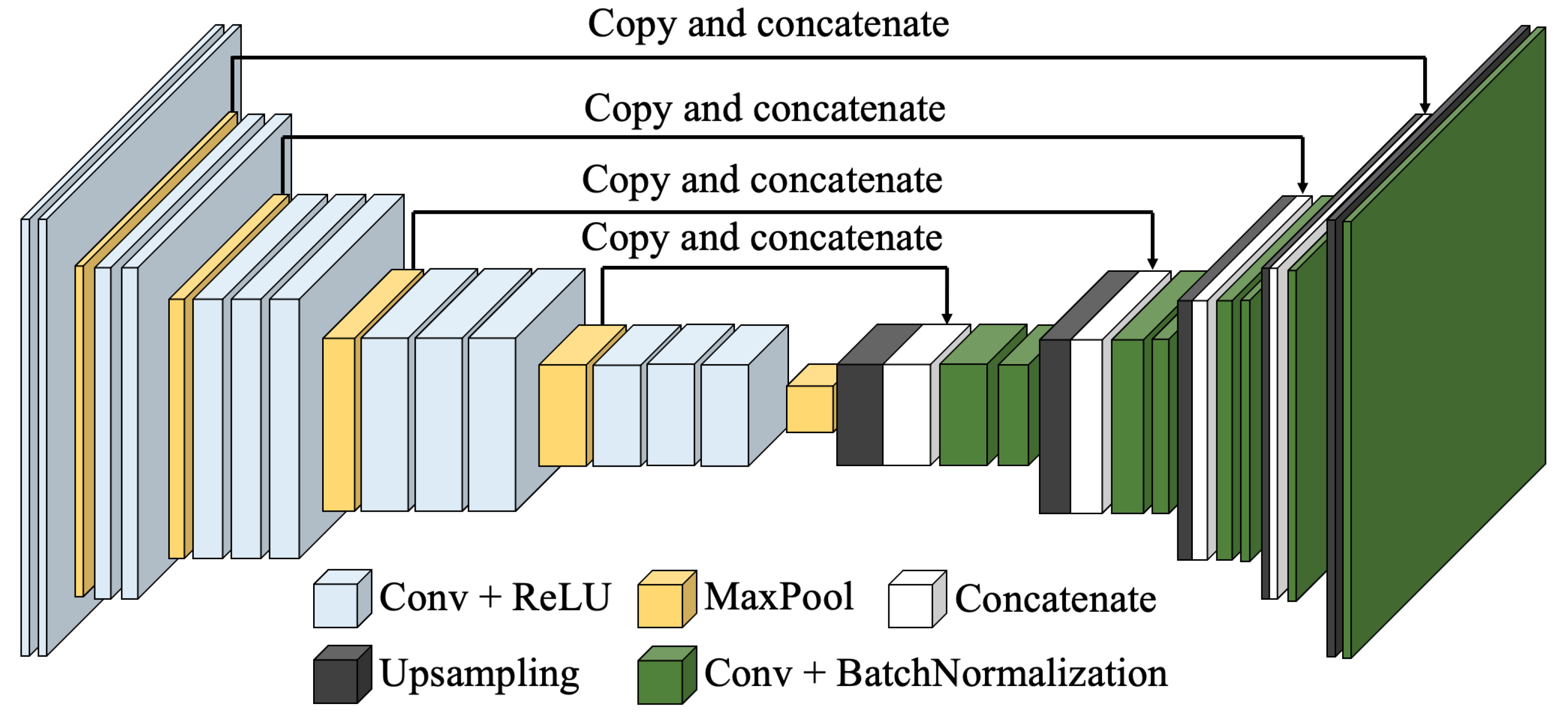
In general, to detect the location of the objects from images, one VGG-Unet architecture consists of two parts. One part using five down-sampling blocks is based on VGG16 structure to capture context. The other part based on U-Net [39] consists five up-sampling blocks and uses a symmetric expanding path to make precise localization enable. Figure 1 shows the architecture of VGG-Unet. This section introduces the details or backgrounds of the layers used in the VGG-Unet.

As VGG16, the input size of the images is 224 × 224 pixels with three channels (Red, Green and Blue) in VGG-Unet. In architecture of VGG-Unet, down-sampling is combined from Convolutional (Conv) layers connected with the Rectified Linear Unit (ReLU) layer and Maxpooling layer, while up-sampling block is consisted of Upsampling layer and convolutional layer, which is followed by an auxiliary layer named Batch Normalization (BN) layer. During the process of up-sampling block, some layers are copied and then concatenated with the output of convolutional layer. After the data calculated through a down-sampling block, the width and height becomes half. The up-sampling block can double the width and height of the input. The detail of each layers is shown in

Table 1. The detailed configuration and specifications of VGG-Unet.

Layer	Type	Pad	Kernel Size	Stride	Output Size	Note
1	Input	-	-	-	224 × 224 × 3
2	Conv + ReLU	1	3 × 3 × 64	1	224 × 224 × 64	down-sampling block 1
3	Conv + ReLU	1	3 × 3 × 64	1	224 × 224 × 64
4	MaxPooling	0	2 × 2	2	112 × 112 × 64
5	Conv + ReLU	1	3 × 3 × 128	1	112 × 112 × 128	down-sampling block 2
6	Conv + ReLU	1	3 × 3 × 128	1	112 × 112 × 128
7	MaxPooling	0	2 × 2	2	56 × 56 × 128
8	Conv + ReLU	1	3 × 3 × 256	1	56 × 56 × 256	down-sampling block 3
9	Conv + ReLU	1	3 × 3 × 256	1	56 × 56 × 256
10	Conv + ReLU	1	3 × 3 × 256	1	56 × 56 × 256
11	MaxPooling	0	2 × 2	2	28 × 28 × 256
12	Conv + ReLU	1	3 × 3 × 512	1	28 × 28 × 512	down-sampling block 4
13	Conv + ReLU	1	3 × 3 × 512	1	28 × 28 × 512
14	Conv + ReLU	1	3 × 3 × 512	1	28 × 28 × 512
15	MaxPooling	0	2 × 2	2	14 × 14 × 512
16	Conv + ReLU	1	3 × 3 × 512	1	14 × 14 × 512	down-sampling block 5
17	Conv + ReLU	1	3 × 3 × 512	1	14 × 14 × 512
18	Conv+ReLU	1	3 × 3 × 512	1	14 × 14 × 512
19	MaxPooling	0	2 × 2	2	7 × 7 × 512
20	Upsampling	-	-	-	14 × 14 × 512	up-sampling block 1
21	Concatenate	-	-	-	14 × 14 × 1024
22	Conv + BN	1	3 × 3 × 512	2	14 × 14 × 512
22	Conv + BN	1	3 × 3 × 256	2	14 × 14 × 256
23	Upsampling	-	-	-	28 × 28 × 256	up-sampling block 2
24	Concatenate	-	-	-	28 × 28 × 512
25	Conv + BN	1	3 × 3 × 256	2	28 × 28 × 256
26	Conv + BN	1	3 × 3 × 128	2	28 × 28 × 128
27	Upsampling	-	-	-	56 × 56 × 128	up-sampling block 3
28	Concatenate	-	-	-	56 × 56 × 256
29	Conv + BN	1	3 × 3 × 128	2	56 × 56 × 128
30	Conv + BN	1	3 × 3 × 64	2	56 × 56 × 64
31	Upsampling	-	-	-	112 × 112 × 64	up-sampling block 4
32	Concatenate	-	-	-	112 × 112 × 128
33	Conv + BN	1	3 × 3 × 64	2	112 × 112 × 64
34	Upsampling	-	-	-	224 × 224 × 64	up-sampling block 5
35	Conv + BN	1	3 × 3 × 3	2	224 × 224 × 3
36	Output	-	-	-	224 × 224 × 3

.

3.1.2. Layers

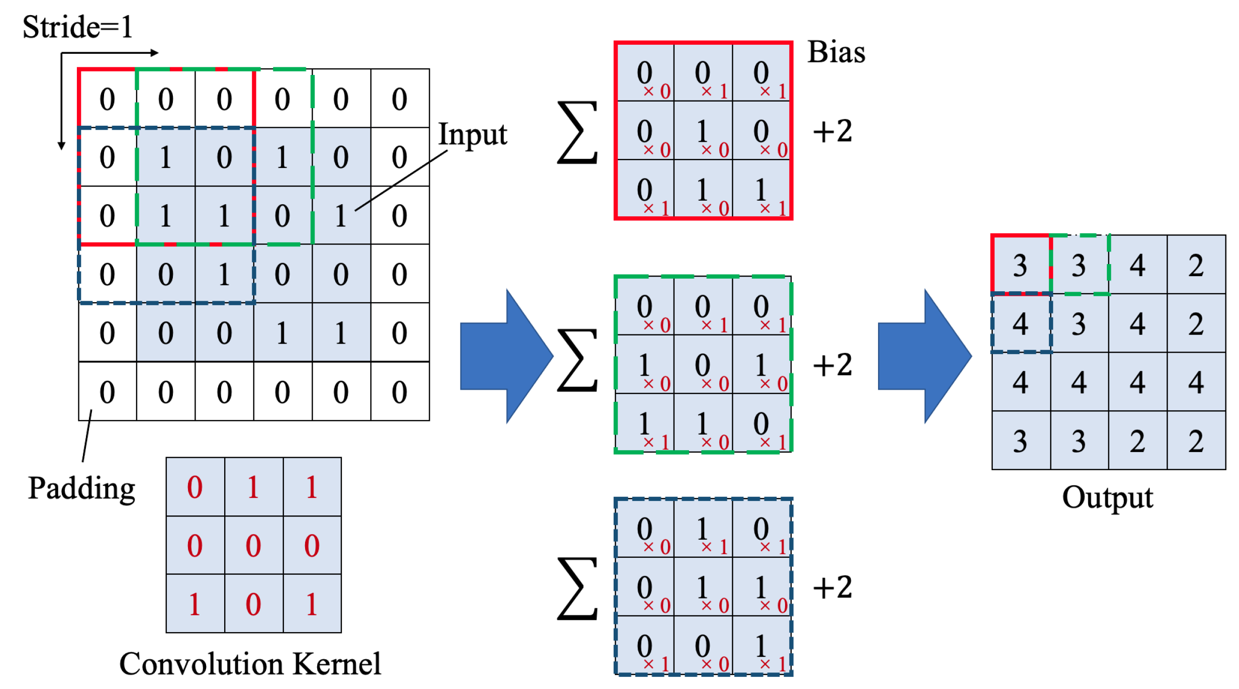
The essence of deep learning is to extract the features of the detected object. The most important step to carry out this process is convolution, by Convolutional layers. Convolutional layers are adopted in both down- and up-sampling blocks. A set of kernels with learnable weight to perform the convolution operation are used in the layer, as shown in Figure 2. Each kernel slides on the input array with a specific step size defined as stride and the convolution implemented by this process. The multiplications are done between the element from kernel and the element from subarray of input to get a receptive field. Then the multiplied values are summed with bias added to get a value in the output array. To maintain the output size is equal to the input size, adopt zero-padding (Pad) for the input array. The output size of a convolutional layer depends on the size of input, Pad numbers, kernel size, and stride, which can be calculated as the example in Figure 2.

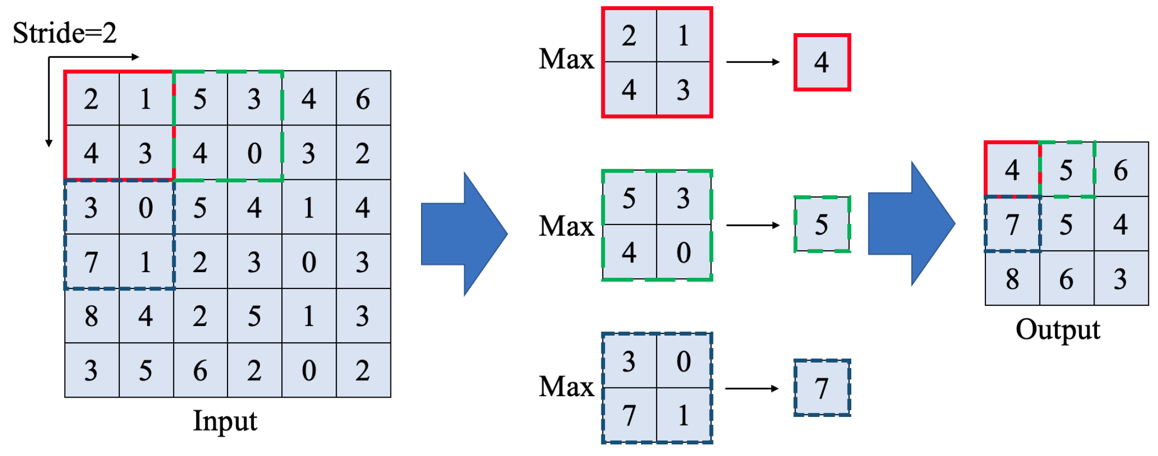
Another key aspect in VGG-Unet is Maxpooling layer, which reduces the spatial size of the input array and often defined as downsampling. It uses a subarray to get the max values. Figure 3 shows the example of MaxPooling layer with a stride of two. Hence, once the input array goes pass the Maxpooling layer, the width and height become half. Once the array go through Maxpooling layer, the memory becomes a quarter of the original one. This can release more memory for more calculation and the training efficiency is significantly improved.

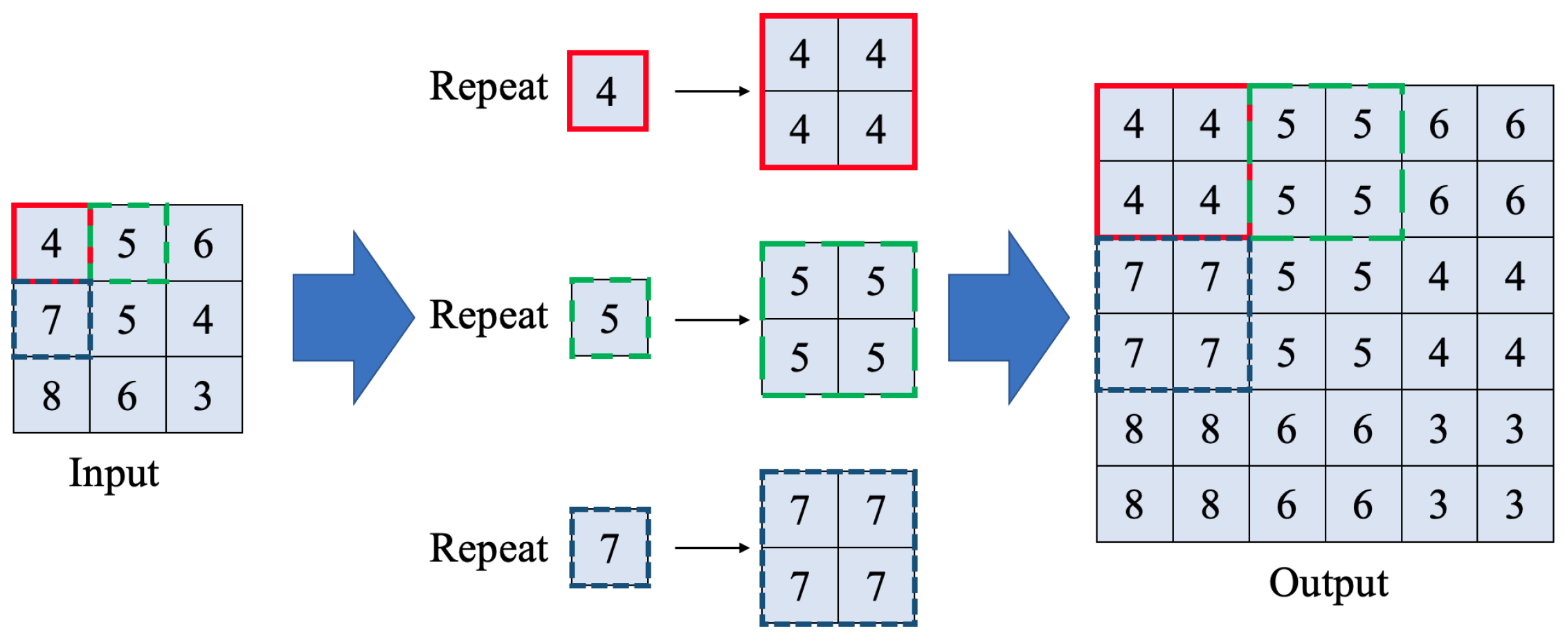
The largest difference between CNN and FCN is up-sampling blocks, which replaces the position of the neural layer in CNN. Up-sampling blocks are adopted to make the feature array back to pixels in three channels, which is called image visualization. Upsampling layer is widely used in the up-sampling blocks. It increases the width and height from the input array. Any element in the input array would be repeated in two directions, shown as Figure 4. Every time after upsampling, resolution would become 2 × 2 of the input array. Since the number of Up-Sampling layers and MaxPooling layers are same, the input and output size of images are same.

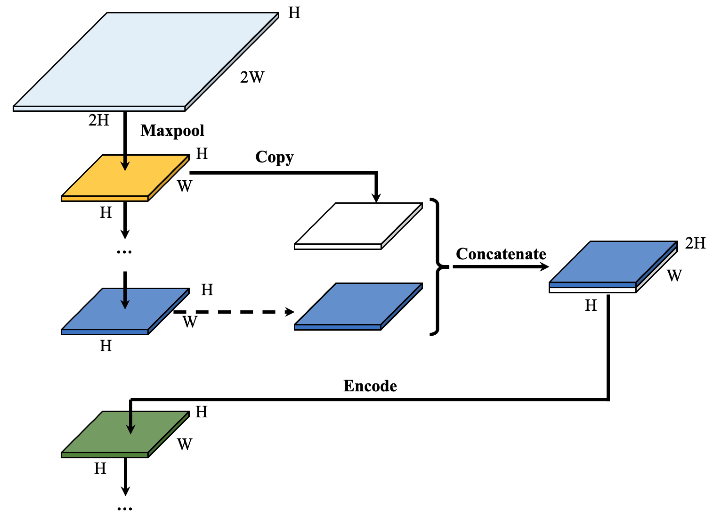
Copying and concatenating for layers come from U-net and is a unique feature that different from other FCNs. The output of convolutional layers can catch the objects’ features into abstract information, and then the outputs can be transferred into spatial information to make annotations by the up-sampling blocks. However, Convolutional layers and Pooling layers will lose spatial information, which is more serious in the pooling process. For image segmentation, spatial information and abstract information are equally important. Thus, traditional FCN don’t have good results and high accuracies. Since each time pooling process will seriously lose spatial information, to solve the problem, Copying and concatenating are proposed to connect the features in down-sampling blocks to the corresponding up-sampling blocks in U-net. Figure 5 shows the process of copying and concatenating during down- and up-sampling in VGG-Unet.

3.2. Process of Training and Predicting

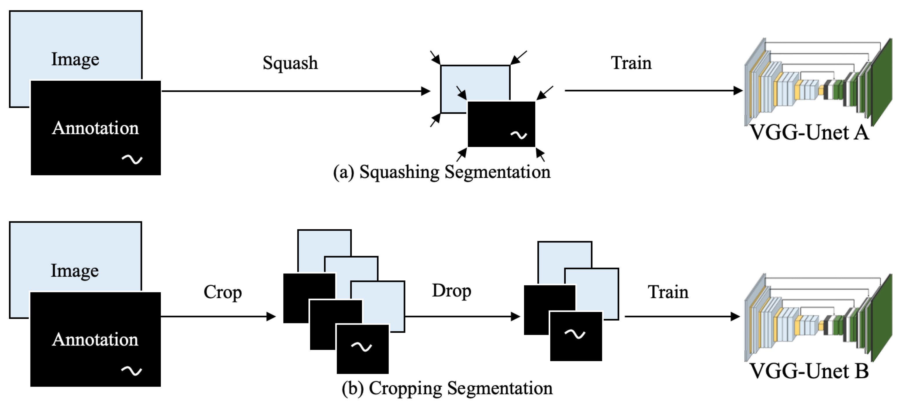
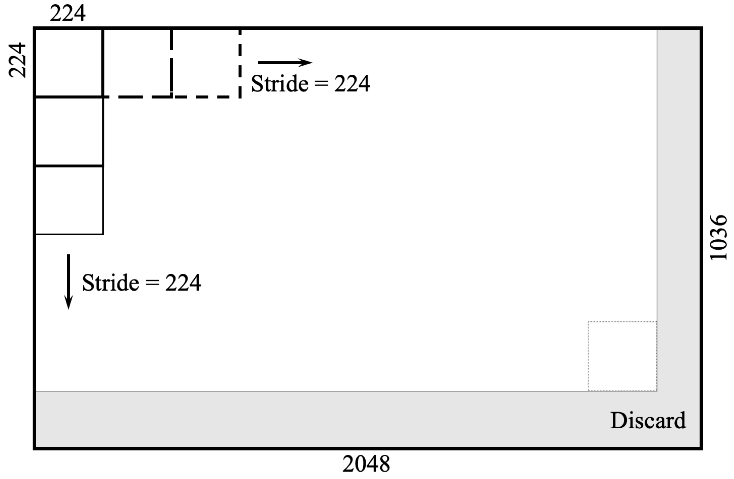
Traditional semantic Deep Learning methods come from definition of computer science serval years ago and then adopted into engineering area until then. Input images of these methods tend to be lower resolutions because of the hardware limitations. However, with the development of hardware especially cameras, GPUs and monitors, 4 k or even higher resolution images are possibly taken and more conveniently and fluently shown to people. Due to Damage Segmentation is pixel-level damage detection, some improvement for input data should be taken into consideration to use these Deep Learning methods. Here are two methods for Damage Segmentation and the processes of training is shown as Figure 6. One method is called Squashing Segmentation and to input full images which are squashed into 224 × 224 pixels before training process, whatever original sizes are. This is traditional semantic segmentation for object. Notably, this method loses a lot of characteristics information of small objects during process of squashing but remain relationship information between objects. Since cracks are not large enough objects in high resolution images, and just accounts less than 2% of pixels in one image, another method called Cropping Segmentation is adopted to input cropped images with size of 224 × 224 pixels for training. During cropping processes, width and height of small pieces of images are same as stride as 224 pixels, and the left parts less than 224 pixels in width and height of original images are discarded. The schematic of cropping is shown as Figure 7. This method keeps original size of damage pixels while training, avoiding the loss of characteristic information of damages during squashing process. To compare the results of different training methods or input data size, each data set runs 50 epochs. All the described works is based on workstation installed with GPU (NVIDIA Geforce GTX 1080). All the training processes are performed on Ubuntu system and coded by Python 3.6. Virtual environment was established by TensorFlow 1.2 and Keras 2.0.

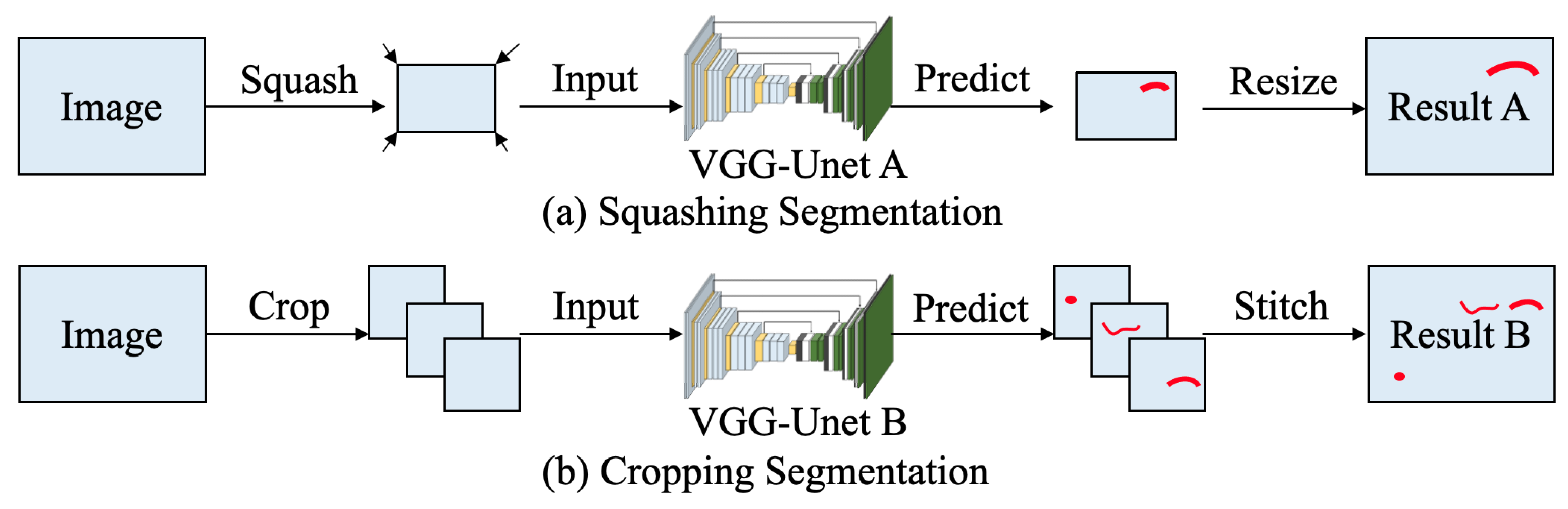
After training different VGG-Unet models under different methods, the next step to do is predicting damages from images of test data set. To compare the performance of different VGG-Unet models, here each data set chooses the best FCN model from 50 epochs to evaluate. The testing process for VGG-Unet model training from Squashing Segmentation is similar as training process, and it inputs squashed images before prediction. After predicting and get outcomes, these predicted images are resized as original images before squashing with same size. And testing process of the other method, Cropping Segmentation, is to input cropped images, whose size is 224 × 224 pixels, for prediction. The outcomes after predicting are stitched back to full images. The processes of prediction are shown as Figure 8.

4. Building Data Set and Choosing Configurations

4.1. Damage Images and Annotations

200 steel images and 500 rubber bearing images are collected from different bridges, under different illuminance conditions and at different shooting angles. Then the damage these images are manually marked by Image Labeler, which is built-in application in MATLAB. After labeling the damages and getting the annotation files, these annotation files are renamed as the same name as original images. After that, images are divided randomly for the next steps. For corrosion images, 80% of images are prepared for training and the other images are both for validation and testing. And for rubber bearing damage detection, 80% of images for training, 10% for validation and the other part is for testing. To compare the difference results of squashed full images and cropped images, images and annotations from the data set are copied and cropped into small images with size of 224 × 224 pixels for Cropping Segmentation, after getting the data set.

Table 2. The proportion of data set after dropping background data.

Damage Class	Image Type	Training	Validation	Testing
Corrosion on steel	Squashed images	160	40	40
	Cropped images	9728	2719	2719
Damage on rubber bearing	Squashed images	400 (193)	50 (22)	50 (27)
	Cropped images	34,626 (1968)	5027 (409)	4218 (261)

shows the detail of data set. Since not all rubber bearing images are with damages, the number in parentheses represents the quantity of images excluded non-damage images.

To compare the influence of different weights of damage pixel in data set, Mean Damage Ratio (MDR), is widely used for evaluating the data set of segmentation. Damage Ratio refers to the number of damage pixels in each image divided by the total number of pixels in the image. The average of these outcomes in the data set is MDR. By calculating, MDR of corrosions is about 30% while MDR of cracks is less than 2%. Thus, corrosion is a kind of large area damage, and crack is a kind of minor damages.

4.2. Evaluation Method for Accuracy

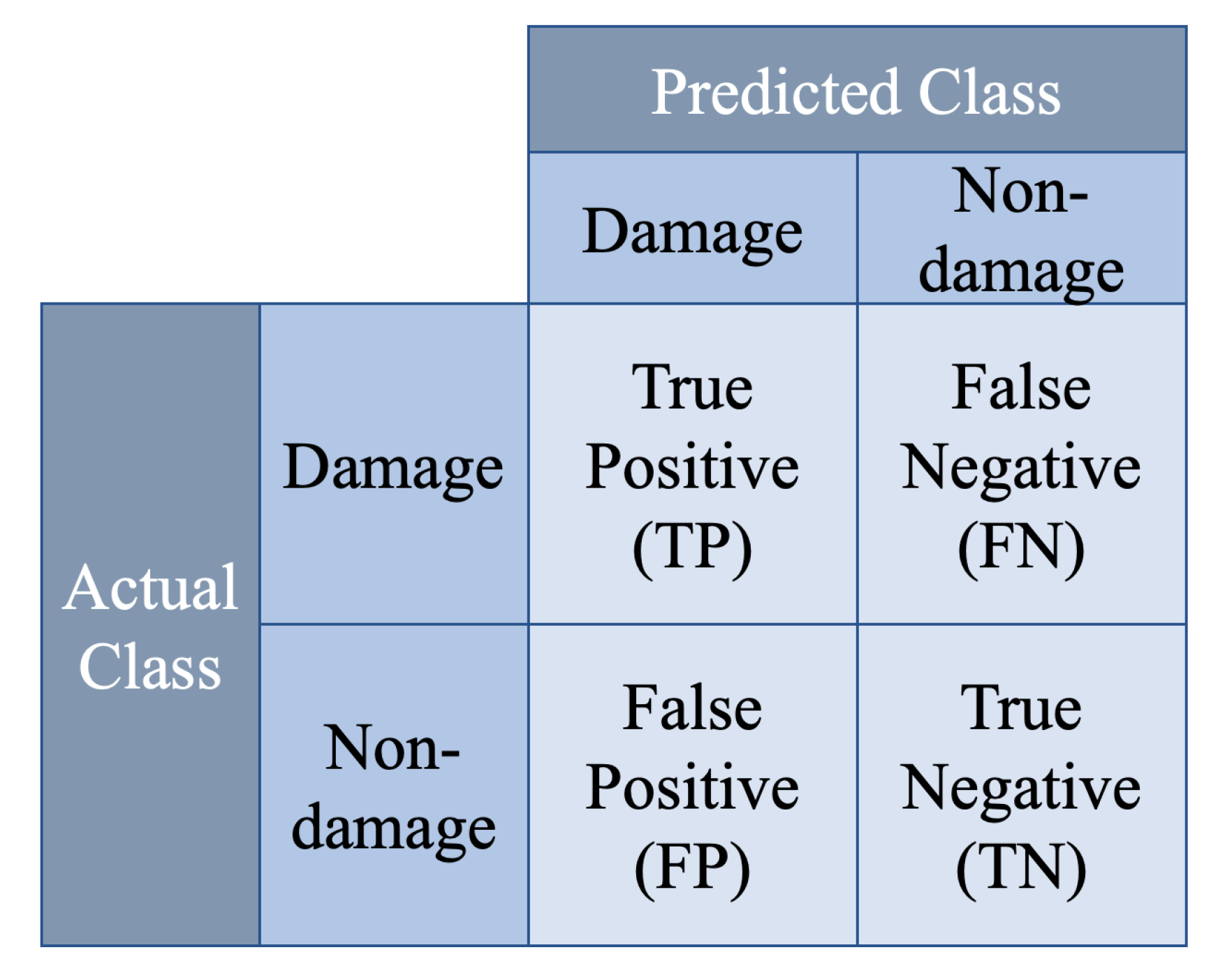
To evaluate accuracy of the outcome, Confusing Matrix is widely used in Deep Learning, especially for classification. However, segmentation calculate accuracy through the number of pixels of each class in one image instead of the quantity of images of each class from all images in the data set. In this research, all VGG-Unet models are trained for two classes segmentation. Thus, the pixels predicted as damages or rubber bearings are counted as Positive, while others are Negative. And if the class of predicted pixels is same as the class in annotation, these pixels are predicted as True while others are False. The name of pixels in Confusing Matrix of Damage Segmentation for two classes is shown as Figure 9.

Many criteria for accessing accuracy of semantic segmentation have been proposed and widely used. Here are 4 popular metrics to evaluate the prediction ability of VGG-Unet model at the level of pixel. Most traditional method is called pixel accuracy (PA), which means calculate the accuracy pixel by pixel and defined as (1). Compared with PA, mean pixel accuracy (MPA) takes quantities of pixels from different classes into account, and it would calculate the average of accuracy of all classes. The (2) shows how to calculate MPA, and here k means the number of true classes in one image. Mean intersection over union (MIoU) and frequency weighted intersection over union (FWIoU) [39], combine the pixels of one class together as one union, shown as (3) and (4). FWIoU also considers the proportion of all classes and select the weight for each class.

$$\mathrm{P}\mathrm{A}=\frac{\mathrm{T}\mathrm{P}+\mathrm{T}\mathrm{N}}{\mathrm{T}\mathrm{P}+\mathrm{F}\mathrm{P}+\mathrm{F}\mathrm{N}+\mathrm{T}\mathrm{N}}$$

(1)

$$\mathrm{M}\mathrm{P}\mathrm{A}=\frac{1}{\mathrm{k}}\left(\frac{\mathrm{T}\mathrm{P}}{\mathrm{F}\mathrm{N}+\mathrm{T}\mathrm{P}}+\frac{\mathrm{T}\mathrm{N}}{\mathrm{F}\mathrm{P}+\mathrm{T}\mathrm{N}}\right)$$

(2)

$$\mathrm{M}\mathrm{I}\mathrm{o}\mathrm{U}=\frac{1}{\mathrm{k}}\left(\frac{\mathrm{T}\mathrm{P}}{\mathrm{F}\mathrm{P}+\mathrm{T}\mathrm{P}+\mathrm{F}\mathrm{N}}+\frac{\mathrm{T}\mathrm{N}}{\mathrm{F}\mathrm{P}+\mathrm{T}\mathrm{N}+\mathrm{F}\mathrm{N}}\right)$$

(3)

$$\mathrm{F}\mathrm{W}\mathrm{I}\mathrm{o}\mathrm{U}=\frac{1}{\mathrm{T}\mathrm{P}+\mathrm{T}\mathrm{N}+\mathrm{F}\mathrm{N}+\mathrm{F}\mathrm{P}}\left(\frac{\mathrm{T}\mathrm{P}\left(\mathrm{T}\mathrm{P}+\mathrm{F}\mathrm{N}\right)}{\mathrm{F}\mathrm{N}+\mathrm{T}\mathrm{P}+\mathrm{F}\mathrm{N}}+\frac{\mathrm{T}\mathrm{N}\left(\mathrm{T}\mathrm{N}+\mathrm{F}\mathrm{P}\right)}{\mathrm{F}\mathrm{P}+\mathrm{T}\mathrm{N}+\mathrm{F}\mathrm{N}}\right)$$

(4)

However, PA and FWIoU don’t enlarge the weight of damages and just calculate from percentage of damage pixels. These two methods are suitable for large area object segmentation such as corrosion or structure, but unreasonable for small damages like cracks, since the undamaged size (TN) of images occupies too many pixels. On the contrary, MPA and MIoU, magnified the weight of damages as same as the weight of other parts. These methods are good for segmentation evaluation for small damages, which just occupy a small proportion of pixels in the images. Thus, these two methods are widely adopted for the data set with carefully selected and processed damage images to judge the capabilities of FCN models on detecting the severity of the minor damages. However, it is not all time that we want to excessively increase the weight of damages, especially for real-word damage inspection. One reason is that most images in the process of inspection do not include damages, while the damage pixels only account a small part in the whole data set. Another reason is humans judge damage from images through the characteristics of continuous pixels rather than a small number of independent pixels. Thus, some independent pixels which are not precisely predicted cannot influence people’s understanding of labeled images, however, it greatly affects the accuracy value. What’s more, using these two methods make the evaluation result fluctuate greatly when the damage occupies different areas in the images. These are caused by excessively increasing the weight of minor damages. To make a balance between no increase damage weight and overly increase damage weight, a method could control the weight of objects is defined. This method is called relative weighted intersection over union (RWIoU) using following equations:

$$\mathrm{\alpha }={\left(\frac{\mathrm{T}\mathrm{P}+\mathrm{F}\mathrm{N}}{\mathrm{T}\mathrm{P}+\mathrm{T}\mathrm{N}+\mathrm{F}\mathrm{N}+\mathrm{F}\mathrm{P}}\right)}^x$$

(5)

$$\mathrm{\beta }={\left(\frac{\mathrm{F}\mathrm{P}+\mathrm{T}\mathrm{N}}{\mathrm{T}\mathrm{P}+\mathrm{T}\mathrm{N}+\mathrm{F}\mathrm{N}+\mathrm{F}\mathrm{P}}\right)}^x$$

(6)

Then,

$$\mathrm{\beta }=\frac{1}{\mathrm{\alpha }+\mathrm{\beta }}\left(\frac{\mathrm{\alpha }\mathrm{T}\mathrm{P}}{\mathrm{F}\mathrm{P}+\mathrm{T}\mathrm{P}+\mathrm{F}\mathrm{N}}+\frac{\mathrm{\beta }\mathrm{T}\mathrm{N}}{\mathrm{F}\mathrm{P}+\mathrm{T}\mathrm{N}+\mathrm{F}\mathrm{N}}\right)$$

(7)

where, x is a rational number and x ∈ (0,1). In this evaluation method, x is the key to magnify the weight of damage pixels by controlling the value of x. If x is equal to 0, RWIoU is same as MIoU while if x is equal to 1, RA is same as FWIoU. Since x is an undetermined value, RWIoU under different value of x is named as RWIoUx.

All the pervious equations for calculation accuracy are used for images containing damages. However, in real life, most images taken by human beings, robots or even UAVs are intact and not contain damages. In this condition, TP and FN are equal to 0 and k is 1 in the research, Thus, PA, MPA, MIoU, FWIoU and RWIoU can be simplified and the final equation is same as following:

$$\mathrm{P}\mathrm{A},\mathrm{M}\mathrm{P}\mathrm{A},\mathrm{M}\mathrm{I}\mathrm{o}\mathrm{U},\mathrm{F}\mathrm{W}\mathrm{I}\mathrm{o}\mathrm{U},\mathrm{R}\mathrm{W}\mathrm{I}\mathrm{o}\mathrm{U}=\frac{\mathrm{T}\mathrm{N}}{\mathrm{F}\mathrm{P}+\mathrm{T}\mathrm{N}}$$

(8)

5. Results and Evaluation

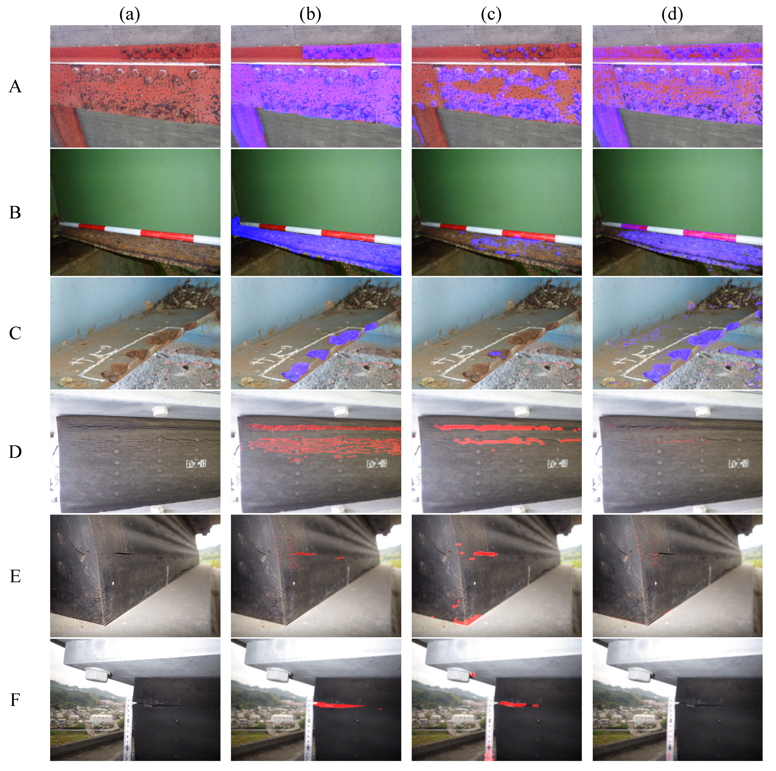
Some prediction results are shown in Figure 10. In the figure, image A, B and C are corrosion image and D, E and F are from rubber bearing data set. These images prove that the VGG-Unet model trained from squashed images could generally identify the location of damage on the rubber bearing, not only for corrosions, but also for rubber bearing cracks, as shown in (c). However, the VGG-Unet model may ignore some pixels of damage because some features of damages are lost during the process of compressing, especially minor damages.

On the contrary, the results trained by Cropping Segmentation have a large gap in the ability to identify corrosions and rubber bearing cracks. The model for corrosion prediction has a good performance on detection corrosions from steel structure, while only a few crack pixels on the rubber bearings are predicted, even though the two VGG-Unet models are trained from the same methodology and hyperparameters. From the experiment of other researchers, the larger data set should help Deep Learning models to reach higher accuracy. The volume of the data set of rubber bearing is several times larger than that of the corrosion data set and the number of damage pixels is not much different, while the detection results have such a large difference. The largest possibility is the differences on proportion of the target object in the whole data set. Due to the damage pixels from the data set don’t have enough percentage during training process, the VGG-Unet model is not so sensitive to them.

The accuracy results are calculated and shown in

Table 3. Accuracy of Damage Segmentation.

Data Set	Method	PA	MPA	MIoU	FWIoU	RWIoU0.1
Corrosion on steel	Squashing	75.6	57.7	44.2	62.7	46.8
	Cropping	81.6	70.4	57.1	71.4	59.1
Damage on rubber bearing	Squashing	99.2 (98.7)	75.8 (55.4)	74.4 (52.7)	98.7 (97.8)	80.7 (64.3)
	Cropping	99.4 (99.0)	73.8 (51.4)	73.4 (50.7)	98.9 (98.0)	79.9 (62.8)

. From the table, it shows that Cropping Segmentation has a better capability on predicting corrosions than Squashing Segmentation, while the results of these two methods are similar when it comes to rubber bearing detection. And the results corrosion prediction from two evaluation methods which don’t enlarge the weight of damage, don’t have a large gap, compared with other two methods of increasing the weight of damages. Nevertheless, if only focus on the rubber bearing images with damages, the evaluation method of enlarging or not enlarging the weight of damage will produce large difference in results. This is because that the TN pixels are accounted for a large proportion and seriously affect the calculation of accuracy under each method. In this case, RWIoU is an alternative method to balance the huge disparity between the evaluation results.The table proves that the balance of the number of pixels in each category in the data set can affect not only the ability of prediction results, but also the accuracy of evaluation results.

6. Pixel-Level Data Balance

6.1. Process

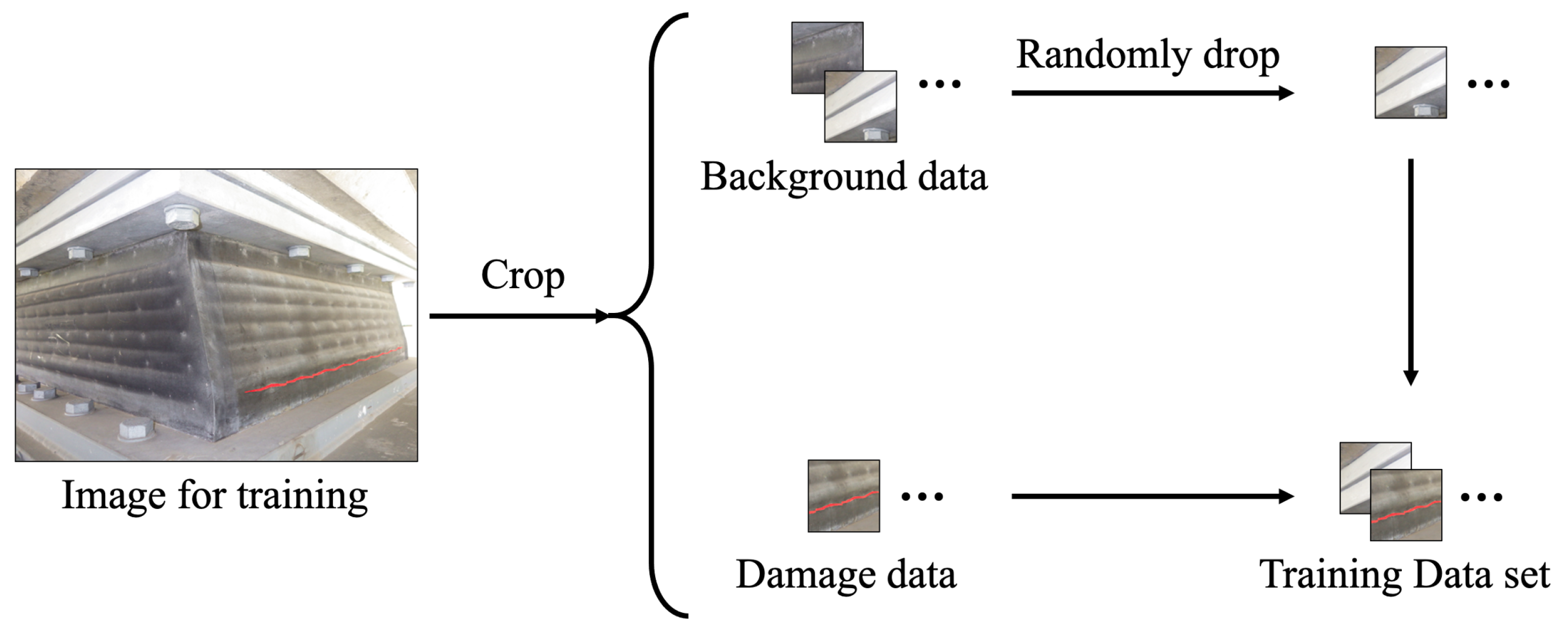
The previous research shows that Cropping Segmentation should have a better performance on detecting objects. To improve the capability of minor damage detection, especially for cracks, Background Data Drop Rate (BDDR) is defined to control the proportion of pixels in each category from the training and validation data set. BDDR means the percentage of randomly dropped out images in the background. The example of dropping background data is shown as Figure 11. After cropping original images, the background images are automatically separated from the data set by Python code, by counting whether there are labeled pixels from the corresponding annotations. If there are no pixels labeled as damage from annotation file, the cropped images are ragarded as background images. Then these background images are randomly deleted from the data set, according to the given BDDR. After that, the left images are mixed with damage data to be a new data set for training VGG-Unet model. In this research, the testing data set isn’t changed, due to it is not used in training the VGG-Unet model and does’t effect the accuracy of the model.

The original data set is the cropped images from rubber bearing, which is shown in Table 2 as above. Another four different BDDR parameters are tested: 0.2, 0.5, 0.8 and 0.9.

Table 4. The proportion of data set for segmentation.

Value of BDDR	Training	Validation	Testing
0	34,626 (1968)	5027 (409)	4218 (261)
0.2	28,094 (1968)	4103 (409)
0.5	18,297 (1968)	2718 (409)
0.8	8499 (1968)	1332 (409)
0.9	5233 (1968)	870 (409)

shows the detail of data set and the number in parentheses represents the quantity of images with damage. By enlarging the value of BDDR, the percentage of damage images is becoming larger and larger.

The MDR of data set for Damage Segmentation is shown in

Table 5. MDR of data set after dropping background data.

Value of BDDR	All	Training	Validation	Testing
0	0.008 (0.130)	0.007 (0.123)	0.016 (0.194)	0.005 (0.081)
0.2	0.009 (0.130)	0.009 (0.123)	0.019 (0.194)
0.5	0.014 (0.130)	0.013 (0.123)	0.029 (0.194)
0.8	0.024 (0.130)	0.028 (0.123)	0.059 (0.194)
0.9	0.033 (0.130)	0.046 (0.123)	0.091 (0.194)

. From the table, it can be found that with the increasing of BDDR, MDR also increases a lot, from 0.7% to 4.6% for training data set and from 1.6% to 9.1% for validation data set.

6.2. Results

All accuracy outcomes of different data set under different BDDR by different evaluation methods are shown in

Table 6. All results of evaluation method.

Data Set	BDDR	PA (%)	MPA (%)	MIoU (%)	FWIoU (%)	RWIoU0.1 (%)
All images (50)	0	99.439	73.755	73.382	98.907	79.905
	0.2	99.493	75.715	75.318	99.016	81.412
	0.5	99.451	78.761	77.104	99.014	82.753
	0.8	99.048	85.457	78.515	98.655	83.745
	0.9	99.374	82.013	78.433	98.974	83.747
Damage images only (27)	0	98.969	51.405	50.715	97.983	62.795
	0.2	99.079	55.046	54.311	98.196	65.595
	0.5	99.023	60.707	57.639	98.214	68.101
	0.8	98.596	73.428	60.571	97.868	70.256
	0.9	98.986	66.835	60.206	98.244	70.047

. In the Table, it can be found that with increasing of BDDR, MPA and MIoU increase a lot while PA and FWIoU don’t change obviously, because MPA and MIoU enlarge the weight of damage pixels as same as the weight of non-damage pixels. This proves that more reasonable BDDR could improve the capability of predicting damages from images of rubber bearings and evaluation method to increase the weight of objects is necessary especially the objects occupy few pixels of whole data set, such as MPA and MIoU. The results of all images are better than which exclude images without damages. This is because of the lower percentage of pixels of damage after taking images without damages into account. Since most of rubber bearings are intact while inspection in real life, the results would be much higher than those in Table 6.

While setting x is equal to 0.1, RWIoU0.1 shows similar result as MIoU. And results FWIoU and RWIoU0.1 under BDDR of 0.8 are all higher than these under BDDR of 0.9, while FWIoU is a little lower. This is because the VGG-Unet model trained from Cropping Segmentation under BDDR of 0.9 is too sensitive to damages that it sometimes misjudges pixels near damages as damage pixels, even though it may have a better performance of predicting background. And enlarging weight of damages cause the pervious evaluation results. As comparing MIoU results of all images and images with damages, when about half of images including damages, MIoU result has 18% difference while RWIoU0.1 has 13.5% difference. This difference would be lower if x is larger. Since using RWIoU could decrease the difference, under condition of different damage image proportion, it could be taken for accuracy evaluation for segmentation especially in real life.

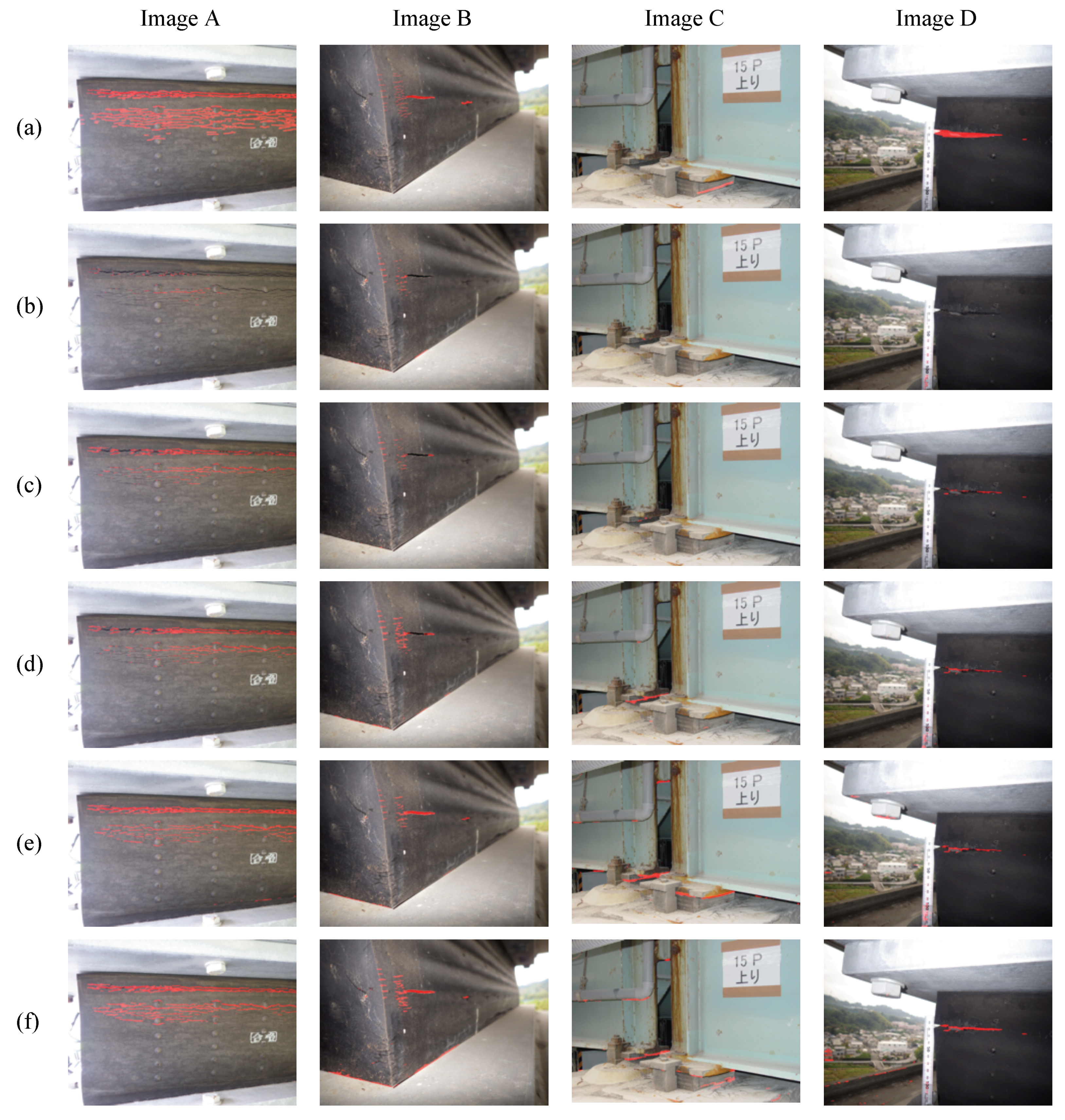
Figure 12 shows some typical examples for rubber bearing inspection. (a) is ground truth, which means manually labeled images, and from (c) to (g) are results of Cropping Segmentation under different BDDR. Image A is the image of seriously damaged rubber bearing, and it is taken almost from a positive angle to the surface of rubber bearing and very similar to the images in the traditional data set for segmenting damages. Without too many interferences of background, image A could show the capability of damage prediction. Image B simulates the angle of view while inspect structures in the narrow space, since the filming angle is very small from the object’s surface and the distances of rubber surface to camera lens are different. Image C is the rubber bearing photo taken in a long distance and in it the rubber bearing only occupy a small area. And Image D shows one wide crack on the rubber bearing, and it is taken with the condition that half of pixels are from background, such as trees and buildings. This condition would interfere the results of object recognition and generate some noise.

These images prove that with BDDR increases, the capability of damage prediction becomes stronger and stronger, with nearly most pixels of damages could be predicted and labeled. However, in the training data set, the VGG-Unet models are also a little more sensitive to background, especially pixels on the boundaries, in darker colors or under lower illuminance. Thus, from Figure 12 it proves that segmentation results are exact while BDDR is 0.8.

7. Conclusions

This paper uses segmentation method to detect corrosions from steel bridges and cracks from rubber bearings, based on VGG-Unet. The model to detect corrosions have a good performance while the capability of model for rubber bearing damage detection needs to be improved. Then, by evaluating the prediction results, a possibility is proposed that the proportion of pixels of each category in the data set will reduce the accuracy of damage recognition. To verify the idea and improve the model’s capability of detecting rubber bearing damages, Background Data Drop Rate (BDDR) is defined to control the proportion of damage pixels from each data set. Different from traditional method to improve accuracy of models by adding more images to the data set, the data-dropping method improves the damage recognition ability of VGG-Unet models by reducing the amount of other pixels. Here summarize the conclusions as follows:

• Squashing Segmentation is conducive to detection of the overall position of the damage. However, compared with Cropping Segmentation, this method doesn’t have a good performance on detecting damages’ precise location, due to some feature information are lost during the compressing process before training.
• The damage detection capability of Cropping Segmentation is largely affected by the concentration of valid data in the data set. If the percentage of damage is very low, the VGG-Unet model may be too sensitive to the background pixels, which leads to the low accuracy.
• If the data sets are with low MDR, there is a large gap between different evaluation methods that enhance the weight of damages or not. In this case, FWIoU can be used to make a balance between these different evaluation methods and reduce the gap while expending the weight of minor damage.
• BDDR is an effective parameter to control the proportion of damage pixels in the data set and improve VGG-Unet model’s capability on detecting minor damages. In this research, BDDR of 0.8 has the highest accuracy, slightly stronger than BDDR of 0.9. It shows that a data set with an appropriate concentration of damage pixels is more helpful to train a higher-precision VGG-Unet model.

In the future, more values of BDDR need to be tested to find the best proportion of damage pixels on training for Cropping Segmentation. Besides, due to the models trained in this research is only for single category of Damage Segmentation, models for multiple categories of damage detection also needs to be trained and the method of dropping data to make a balance between all categories of damage pixels is necessary to be researched.

References

- Inoue, M.; Fujino, Y. Social impact of a bridge accident in Minnesota, USA. JSCE Proc. F 2010, 66, 14–26. (In Japanese) [Google Scholar]
- Ministry of Land, Infrastructure, Transport, and Tourism. White Paper on Present State and Future of Social Capital Aging Infrastructure Maintenance Information; Ministry of Land, Infrastructure, Transport, and Tourism: Tokyo, Japan, 2016. (In Japanese)
- Pan, Y.; Feng, D. Current status of domestic bridges and problems to be solved. China Water Transp. 2007, 7, 78–79. (In Chinese) [Google Scholar]
- Graybeal, B.A.; Phares, B.M.; Rolander, D.D.; Moore, M.; Washer, G. Visual inspection of highway bridges. J. Nondestruct. Eval. 2002, 21, 67–83. [Google Scholar] [CrossRef]
- Hoskere, V.; Narazaki, Y.; Hoang, T.A.; Spencer, B.F., Jr. Towards automated post-earthquake inspections with deep learning-based condition-aware models. arXiv 2018, arXiv:1809.09195. [Google Scholar]
- Gao, Y.; Mosalam, K.M. Deep transfer learning for image-based structural damage recognition. Comput. Aided Civ. Infrastruct. Eng. 2018, 33, 748–768. [Google Scholar] [CrossRef]
- Koch, C.; Georgieva, K.; Kasireddy, V.; Akinci, B.; Fieguth, P. A review on computer vision based defect detection and condition assessment of concrete and asphalt civil infrastructure. Adv. Eng. Inf. 2015, 29, 196–210. [Google Scholar] [CrossRef] [Green Version]
- Abdel-Qader, I.; Abudayyeh, O.; Kelly, M.E. Analysis of edge-detection techniques for crack identification in bridges. J. Comput. Civil Eng. 2003, 17.4, 255–263. [Google Scholar] [CrossRef]
- Nishikawa, T.; Yoshida, J.; Sugiyama, T.; Fujino, Y. Concrete crack detection by multiple sequential image filtering. Comput. Aided Civ. Infrastruct. Eng. 2012, 27, 29–47. [Google Scholar] [CrossRef]
- German, S.; Brilakis, I.; DesRoche, R. Rapid entropy-based detection and properties measurement of concrete spalling with machine vision for post-earthquake safety assessments. Adv. Eng. Inf. 2012, 26, 846–858. [Google Scholar] [CrossRef]
- Kaiser, G. The fast Haar transform. IEEE Potent. 1998, 17, 34–37. [Google Scholar] [CrossRef]
- Nussbaumer, H.J. The fast Fourier transform. In Fast Fourier Transform and Convolution Algorithms; Springer: Berlin/Heidelberg, Germany, 1981; pp. 80–111. [Google Scholar]
- Koziarski, M.; Cyganek, B. Image recognition with deep neural networks in presence of noise–dealing with and taking advantage of distortions. Integrated Comput. Aided Eng. 2017, 24, 337–349. [Google Scholar] [CrossRef]
- Jiang, X.; Adeli, H. Pseudospectra, MUSIC, and dynamic wavelet neural network for damage detection of highrise buildings. Int. J. Numer. Methods Eng. 2007, 71.5, 606–629. [Google Scholar] [CrossRef]
- Butcher, J.B.; Day, C.R.; Austin, J.C.; Haycock, P.W.; Verstraeten, D.; Schrauwen, B. Defect detection in reinforced concrete using random neural architectures. Comput. Aided Civ. Infrastruct. Eng. 2014, 29, 191–207. [Google Scholar] [CrossRef]
- Simonyan, K.; Zisserman, A. Very deep convolutional networks for large-scale image recognition. arXiv 2014, arXiv:1409.1556. [Google Scholar]
- Krizhevsky, A.; Sutskever, I.; Hinton, G.E. Imagenet classification with deep convolutional neural networks. Adv. Neural Inf. Process. Syst. 2012, 1097–1105. [Google Scholar] [CrossRef]
- He, K.; Zhang, X.; Ren, S.; Sun, J. Deep residual learning for image recognition. In Proceedings of the IEEE Conference on Computer Vision and Pattern Recognition, Las Vegas, NV, USA, 26 June–1 July 2016; pp. 770–778. [Google Scholar]
- Szegedy, C.; Liu, W.; Jia, Y.; Sermanet, P.; Reed, S.; Anguelov, D.; Erhan, D.; Vanhoucke, V.; Rabinovich, A. Going deeper with convolutions. In Proceedings of the IEEE Conference on Computer Vision and Pattern Recognition, Boston, MA, USA, 7–12 June 2015; pp. 770–778. [Google Scholar]
- Huang, G.; Liu, Z.; Van Der Maaten, L.; Weinberger, K.Q. Densely connected convolutional networks. In Proceedings of the IEEE Conference on Computer Vision and Pattern Recognition, Honolulu, HI, USA, 21–26 July 2017; pp. 4700–4708. [Google Scholar]
- Cha, Y.J.; Choi, W.; Büyüköztürk, O. Deep learning-based crack damage detection using convolutional neural networks. Comput. Aided Civ. Infrastruct. Eng. 2017, 32, 361–378. [Google Scholar] [CrossRef]
- Zhang, L.; Yang, F.; Zhang, Y.D.; Zhu, Y.J. Road crack detection using deep convolutional neural network. In Proceedings of the IEEE Conference on Computer Vision and Pattern Recognition, Phoenix, AZ, USA, 25–28 September 2016; pp. 3708–3712. [Google Scholar]
- Soukup, D.; Huber-Mörk, R. Convolutional neural networks for steel surface defect detection from photometric stereo images. In International Symposium on Visual Computing; Springer: Berlin/Heidelberg, Germany, 2014; pp. 668–677. [Google Scholar]
- Ren, S.; He, K.; Girshick, R.; Su, J. Faster r-cnn: Towards real-time object detection with region proposal networks. IEEE Trans. Pattern Anal. Mach. Intell. 2016, 39, 1137–1149. [Google Scholar] [CrossRef] [Green Version]
- Wang, W.; Wu, B.; Yang, S.; Wang, Z. Road damage detection and classification with Faster R-CNN. In Proceedings of the 2018 IEEE International Conference on Big Data (Big Data), Seattle, WA, USA, 10–13 December 2018; pp. 5220–5223. [Google Scholar]
- Deng, J.; Lu, Y.; Lee, V.C.S. Concrete crack detection with handwriting script interferences using faster region-based convolutional neural network. Comput. Aided Civ. Infrastruct. Eng. 2020, 35, 373–388. [Google Scholar] [CrossRef]
- Wang, N.; Zhao, X.; Zhao, P.; Zhang, Y.; Zou, Z.; Ou, J. Automatic damage detection of historic masonry buildings based on mobile deep learning. Autom. Constr. 2019, 103, 53–66. [Google Scholar] [CrossRef]
- LuqmanAli, W.K.; Chaiyasarn, K. Damage Detection and Localization in Masonry Structure using Faster Region Convolutional Networks. Int. J. 2019, 17, 98–105. [Google Scholar]
- Cha, Y.J.; Choi, W.; Suh, G.; Mahmoudkhani, S.; Büyüköztürk, O. Autonomous structural visual inspection using region-based deep learning for detecting multiple damage types. Comput. Aided Civ. Infrastruct. Eng. 2018, 33, 731–747. [Google Scholar] [CrossRef]
- Redmon, J.; Farhadi, A. YOLO9000: Better, faster, stronger. In Proceedings of the IEEE Conference on Computer Vision and Pattern Recognition, Honolulu, HI, USA, 21–26 July 2017; pp. 7263–7271. [Google Scholar]
- Zhang, C.; Chang, C.C.; Jamshidi, M. Bridge Damage Detection using a Single-Stage Detector and Field Inspection Images. arXiv 2018, arXiv:1812.10590. [Google Scholar]
- Chen, L.C.; Papandreou, G.; Kokkinos, I.; Murphy, K.; Yuille, A.L. Semantic image segmentation with deep convolutional nets and fully connected crfs. arXiv 2014, arXiv:1412.7062. [Google Scholar]
- Iglovikov, V.; Shvets, A. Ternausnet: U-net with vgg11 encoder pre-trained on imagenet for image segmentation. arXiv 2018, arXiv:1801.05746. [Google Scholar]
- Ni, F.; Zhang, J.; Chen, Z. Pixel-level crack delineation in images with convolutional feature fusion. Struct. Control Health Monitor. 2019, 26, e2286. [Google Scholar] [CrossRef] [Green Version]
- Li, S.; Zhao, X.; Zhou, G. Automatic pixel-level multiple damage detection of concrete structure using fully convolutional network. Comput. Aided Civ. Infrastruct. Eng. 2019, 34, 616–634. [Google Scholar] [CrossRef]
- Shi, J.; Dang, J.; Zuo, R.; Shimizu, K.; Tsunda, A.; Suzuki, Y. Structural Context Based Pixel-level Damage Detection for Rubber Bearing. Intell. Inf. Infrastruct. 2020, 1, 18–24. [Google Scholar]
- Narazaki, Y.; Hoskere, V.; Hoang, T.A.; Fujino, Y.; Sakurai, A.; Spencer, B.F., Jr. Vision-based automated bridge component recognition with high-level scene consistency. Comput. Aided Civ. Infrastruct. Eng. 2020, 35, 468–482. [Google Scholar] [CrossRef]
- Fawakherji, M.; Youssef, A.; Bloisi, D.; Pretto, A.; Nardi, D. Crop and weeds classification for precision agriculture using context-independent pixel-wise segmentation. In Proceedings of the 2019 Third IEEE International Conference on Robotic Computing (IRC), Naples, Italy, 25–27 February 2019; pp. 146–152. [Google Scholar]
- Garcia-Garcia, A.; Orts-Escolano, S.; Oprea, S.; Villena-Martinez, V.; Garcia-Rodriguez, J. A review on deep learning techniques applied to semantic segmentation. arXiv 2017, arXiv:1704.06857. [Google Scholar]
Figure 1.
Overall architecture of VGG-Unet.
Figure 2.
Example of Convolutional layer.
Figure 3.
Example of MaxPooling layer.
Figure 4.
Example of Upsampling layer.
Figure 5.
Example of copying and concatenating.
Figure 6.
The training process of Damage Segmentation.
Figure 7.
The schematic of cropping.
Figure 8.
The predicting process of Damage Segmentation.
Figure 9.
Confusing Matrix of detection.
Figure 10.
Prediction results: (a) original images, (b) ground truth, (c) Squashing Segmentation results, (d) Cropping Segmentation results.
Figure 11.
Process of dropping background data.
Figure 12.
Examples of prediction results: (a) ground truth, (b) no data drop results, (c) BDDR of 0.2, (d) BDDR of 0.5, (e) BDDR of 0.8, (f) BDDR of 0.9.