1. Introduction
Motivated by the plenty of applications such as laser remote sensing of the atmosphere [
1,
2], time of flight measurements [
3,
4,
5,
6] and visible light communication [
7,
8], light detection and ranging (LiDAR) has become one of the most versatile active remote measurement techniques. In particular, a rush to develop autonomous cars has led to a surge in the field of LiDAR based on time of flight (ToF) techniques. ToF techniques are the basis of LRF (laser rangefinder) systems which measures the time delay between the emission of the laser pulse and the detection of the back-scattered arrival of that pulse. The most commonly used laser types mainly operate at two spectrum bands of around 0.9 µm and 1.5 µm. It is well known that 1.5 µm wavelength is within the eye-safe band due to the fact that water absorption of 1.5 µm is 100 times more than that of 0.9 µm [
9]. Therefore, it requires more power because longer wavelengths suffer more scattering from atmospheric moisture. On the other hand, when we consider Rayleigh scattering which states that scattering is inversely proportional to the fourth power of the wavelength, that means shorter wavelengths scatter more than longer wavelengths, which degrade the performance of laser rangefinder at shorter wavelengths. Also, it is well known that solar radiation is much less than 0.9 µm. Inevitably, cost is another issue when deciding the operational wavelength. Because 0.9 µm is compatible with silicon-based photodetectors (i.e., avalanche photodetectors (APDs) or photomultipliers), it is much more cost-effective than InGaAs detectors. The choice of laser wavelength has many aspects that one needs to consider carefully when designing laser rangefinders.
The cost and performance of Si-based systems make 0.9 µm wavelength the preferred operation band for detectors. In ToF-based systems, the maximum range depends on many factors that include laser power, beam quality, Tx and Rx optics, detector choice, signal processing, etc. In such systems, the net effect is determined by the detection unit where all optical and electrical noise manifests itself as a signal to noise ratio (SNR). Noise in the photodetector is dominated by the readout electronics noise which can be eliminated by amplifying the current in the detector through the avalanche process. APDs with high internal gain are widely used for applications where high speed and low power detection are required such as visible light optical communications based on Si-APD [
10] and laser rangefinders [
11,
12]. In general, APD working in linear mode, that is biased below the breakdown voltage, requires large reverse bias of around 100–200 V in a Silicon APD which are characterized by their gain, quantum efficiency, excess noise, and bandwidth. Improvement in SNR is generally achieved by the process of avalanche multiplication of the photo-generated carriers. However, this multiplication process also creates excess noise in the APD as the gain increases. Therefore, fluctuations in the avalanche multiplication process, the excess noise, generated by the high reverse bias and temperature dependent gain limit the useful range of the gain.
When APD is biased above breakdown voltage, it is working in the so-called Geiger mode which was introduced in 1989 [
13]. In such a condition, the difference between bias voltage and breakdown voltage is called over-voltage. In this sense, single-photon avalanche diodes (SPAD) are APDs but designed to work above breakdown. The physical characteristics of SPADs are well defined in the literature [
14,
15,
16,
17,
18]. SPAD arrays are also known as SiPMs which consist of microcell densities from a few hundreds to a few thousands per mm
2, depending on the size of the microcell. Due to its array structure, a SPAD has low fill factor and currently smaller active areas when compared to APDs. Moreover, because of quenching circuits they become blind (known as dead time) for a while (about 10’s of nanoseconds) when the photon arrives. In ultra-low light applications especially, SPADs offer superior performance to the conventional APDs. In analog SiPMs, each SPAD is connected to its own passive quenching circuits. Naturally, one of the potential applications of SiPMs is the single photon detection for the purpose of photon counting, photon timing and photon imaging [
17].
To our knowledge, long-range capability or test of SiPM with low energy laser in real environment is not reported in the literature. The existing studies [
1,
2,
19] mainly cover the higher energy laser applications using SiPM.
LiDAR has become an increasingly important technology not only in the areas of automotive, 3D-imaging and rangefinder application but also in the atmospheric sciences because of its ability to characterize the atmosphere. Laser light scattered by air molecules and aerosol particles that are suspended are detected by the receivers so that backscatter coefficient profiles can be determined. These aerosols are the indication of atmospheric pollution. The study [
2] shows that employing a pulsed Nd:YAG laser at 532 nm as source, SiPM was shown to be used for elastic-backscatter aerosol LiDAR with a comparable performance to photomultiplier tubes (PMTs). Another researches [
1,
19] are conducted to show the capability of SiPM both photon-counting and analog mode whose performance is compared with PMT for atmospheric applications. In this study, the backscattering coefficients was also successfully demonstrated for both modes.
The SiPM, in terms of overall SNR, was already proven to exhibit better performance in TOF measurements when compared with an APD [
3] which demonstrates outdoor experiments from a distance of 360 m with an SNR of 22. The SNR of the SiPM was higher by at least one order of magnitude than the SNR of the APD in every condition.
In regard to laser source of LRF systems, solid-state lasers are usually preferred, especially for the long-range (>5 km) operation because of available high pulse energies (e.g., up to several mjoules) as well as better beam parameters in comparison to those of semiconductor lasers. However, solid-state lasers impose several drawbacks that prevent them for many practical applications; among drawbacks are high cost, large size, low efficiencies and high electric power consumption. On the other hand, semiconductor lasers, despite of their limited pulse energies (i.e., a few μjoules), promise many practical advantages such as low cost, small volume, ease of integration, high efficiency and low electrical consumption as well as the capability of high-speed modulation. Semiconductor lasers have also some inherent shortcomings such as elliptical beam shapes with fairly large divergence angles and high astigmatism, yet these issues can be managed by proper optic design such as using cylindrical lenses or anamorphic prisms in the Tx and Rx optics for long-range applications. Thus, semiconductor lasers can be used with SiPMs with appropriate optical design to enable a long-range LRF system with cost-effective and small size features as well as an eye-safe capability at 0.9 μm band owing to the capability of low power detection for SiPMs. Here, we report on such a LRF system using commercially available SiPM with multi-pixel architecture and peak power of 90 Watt at 1 kHz and 100 ns for a relatively long-range detection range of >1 km. An experiment showed that a 3 dB improvement in SNR was obtained by the help of a signal extraction algorithm.
In the past two decades, SiPMs have been extensively considered in highly sensitive detection applications due to their low operating voltage, high gain, high photon detection efficiency, photon number resolving capability. SiPMs have rapidly gained attention owing to their superior sensitivity, high gain along with multi-pixel architecture as well as ideal cost and size features. They were first aimed to be used as an alternative to a conventional PMT in nuclear applications [
20,
21]. The SiPM has its own unique performance characterized by the dark count rate (DCR), photon detection probability, hold-off time and after pulsing effects [
13,
22,
23]. SiPMs have now been utilized for a wide range of applications such as LiDAR [
24], fluorescence light detection in biology and physics [
25,
26], high-energy physics [
27], quantum optics [
28,
29] and medical purposes [
30,
31,
32].
The SiPM consists of a dense array of small microcells (SPADs) functioning in Geiger-mode, each one with its integrated passive quenching resistors. These cells are arrayed in a matrix form and connected in parallel, making a common anode and cathode [
33]. When a microcell in the SiPM is activated by the absorbed photon, Geiger avalanche is initiated giving rise to a photocurrent to flow through the microcell. The sum of the photocurrents from each of these individual microcells combines to give an analog output and reading out from anode or cathode is referred to as the standard output [
33]. When the SiPM is biased above breakdown, working in Geiger mode, it produces a photocurrent proportional to the number of cells activated which flows through the sensor from cathode to anode, either of which can be used as a standard output terminal. Reading out from the cathode will give a negative polarity [
33]. In addition to the anode and cathode, a third terminal called the fast output has been developed by On Semiconductors. It is the sum of capacitively coupled outputs from each microcell. The fast output is used to provide information on the number of photons detected since its amplitude is proportional to the number of microcells that are activated. When photons arrive at a pixel, a pulse is generated at its output regardless of the number of photons. If two or more avalanches occur at the same time, the amplitude of the electrical output pulse is equal to the number of avalanches times the amplitude of a single avalanche. Therefore, the height of the output pulse may be said to be proportional to the number of detected photons assuming that noise is neglected [
34]. Then, the SiPM detector signal is the summed output of that 2D array of microcells, providing great sensitivity improvement over APD and PIN diodes. In general, SiPMs are operated in Geiger-mode may provide high gain (i.e., >10
6) at moderate bias voltages (i.e., ~30 V). Operating (bias) voltage (
Vbias) of SiPM is defined as the sum of breakdown voltage (
Vbr) and overvoltage (Δ
V). The gain of a SiPM sensor is defined as the amount of charge created for each detected photon, and is a function of overvoltage and microcell size and can be calculated from the overvoltage, the microcell capacitance
C, and the electron charge,
q [
33]:
One of our motivations is to investigate the long range capability of laser rangefinder based on 905 nm semiconductor laser and SiPM detector. These two combinations offer a very cost-effective solution for a few km laser rangefinders. Therefore, in this work we study the performance of SiPM based on this configuration.
2. Experimental Studies
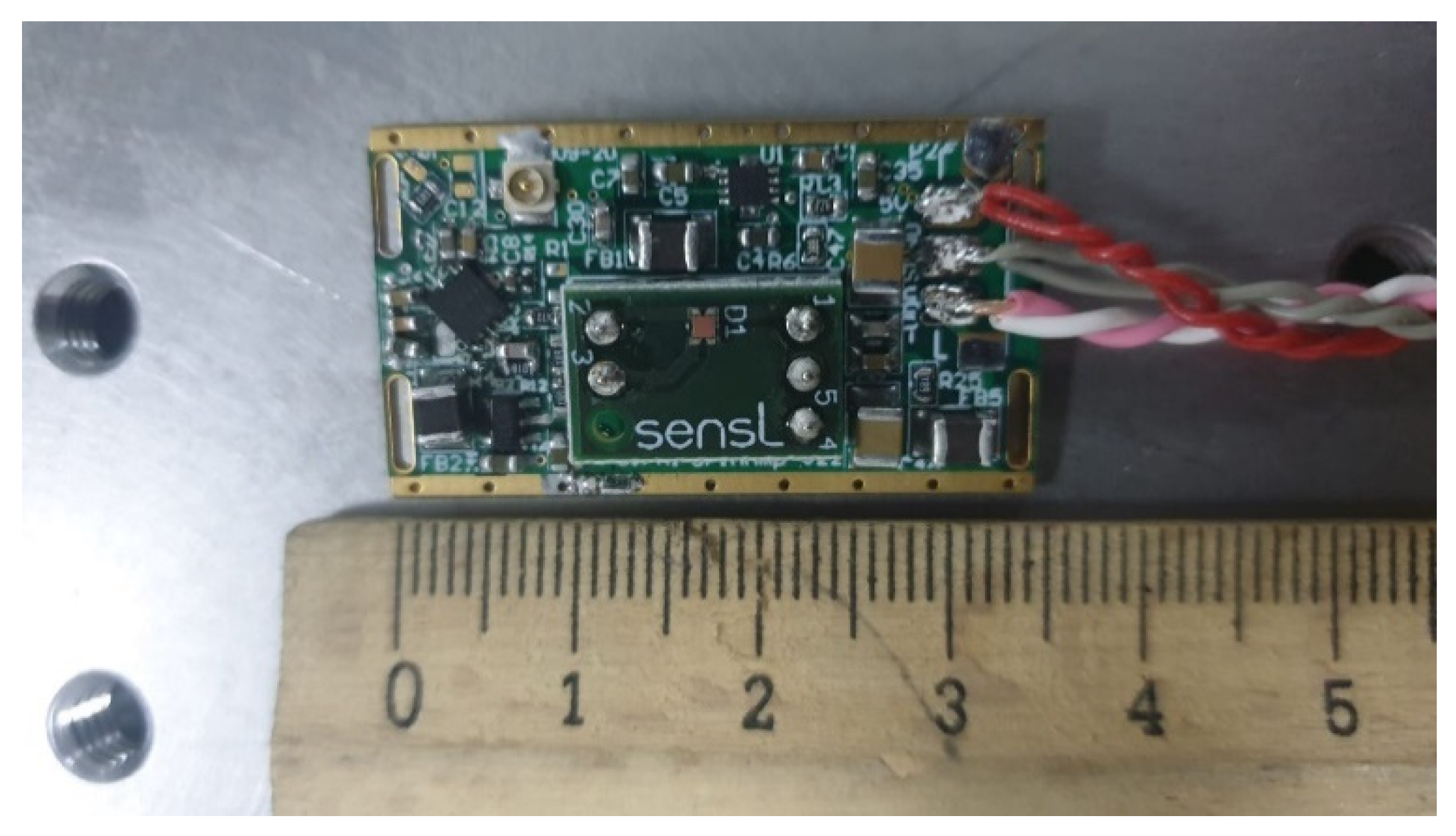
The MICRORB−SMTPA−10020 pin adapter board made by SensL, was used in the receiver. Some important parameters for the SiPM detector used in this work are summarized in the
Table 1. The printed circuit board (PCB) board houses the SiPM sensor and has through-hole pins to allow its use with standard sockets or probe clips [
33]. This sensor was mounted to our designed amplifiers on the PCB board, forming a SiPM-based Rx for our experiments as shown in
Figure 1. In the experiment, the optimum overvoltage in terms of gain and noise level is determined to be 10 Volt, and it remained fixed during the experiments. Therefore, the typical operating (bias) voltage is −33, see
Table 1. In this work, we used a standard output signal which was connected to the amplifier circuit. The fast output was also utilized in order to provide information on the number of photons detected. Although fast output gives much better accuracy of the target on ranging, we consider that fast output signal is difficult to handle in readout electronics since it has both positive and negative sides.
The laser used in this work was the OSRAM SPL PL90-3, operating at a wavelength of 905 nm and providing up to 90 W of peak power. Beam divergences parallel and perpendicular to the axis of propagation were 9 and 25 degrees, respectively. The driver board of the laser was designed by us that consists of a Gallium Nitride field-effect transistors for high-speed switching and discharging capacitors to supply necessary large pulse current. Measured energy at the output of the laser diode is approximately 9 µj at 100 ns pulse width and 1 kHz repetition rate. Note that at the output of the laser rangefinder we lose almost 70% of it because of the large divergence of the laser diode which overfills the aperture.
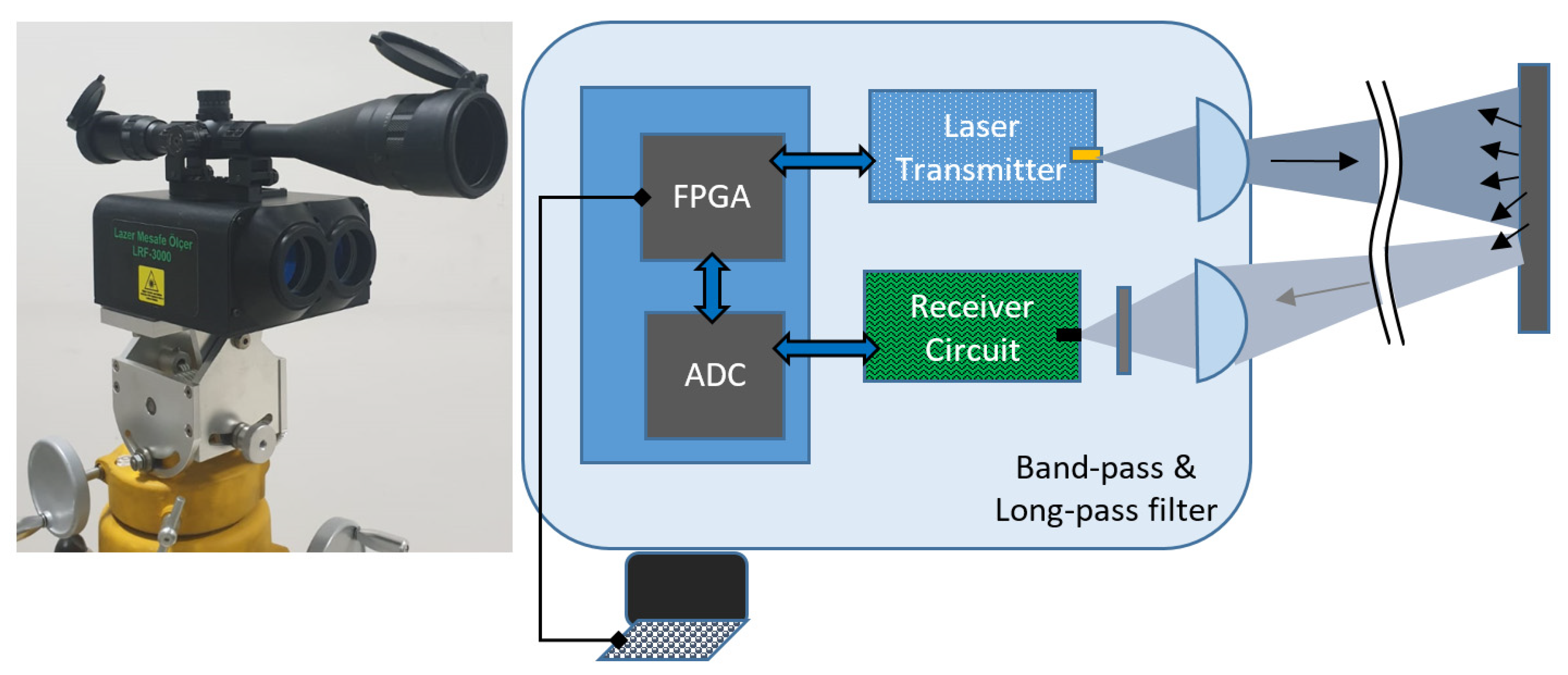
The experiment was performed by using our own prototype shown on the left side of
Figure 2 and on the right is the representation of the setup. Both detector (SiPM) and laser were mounted to the platform which can be slightly adjusted for alignment. The Tx and Rx unit both had the same high precision aspheric lens with a focal length of 100 mm (AL50100-B, Thorlabs, Newton, NJ, USA) and its design wavelength was 780 nm. These lenses which have anti-reflection coating between 650 nm and 1050 nm are 50 mm in diameter with an f-number of 2. They are mounted such that their plain sides facing the laser and detector. Collimated laser beam is in line-rectangular shape and its long edge divergence is approximately 3 mrad (full angle). Receiver full angle field of view (FOV) is calculated as 10 mrad. When we consider the single pixel size, then we obtain instantaneous FOV of 0.2 mrad which corresponds to 20 cm × 20 cm area at 1 km distance for single pixel. In one of our measurement, we used a black wooden target of size 2 by 2 m. The measured distance for this target was 1880 m. Laser spot size on this target was about 5.5 m when the full angle divergence was taken. However, angular field of view of the receiver was 18 m which is larger than the target and the laser spot. In this case the background noise increased which degraded the SNR. Therefore, both transmitter and receiver optics needed to be optimized further. In the test area, direct sunlight and background infrared (IR) radiation degraded the performance of the receiver. Therefore, in front of the receiver, to effectively filter out background light, a band-pass (FL905-10, Thorlabs) and long-pass filters (FEL850-10, Thorlabs) were mounted as close as to each other. Then, the total transmittance of the filters drops to 56%.
In this work, for all experiments, the laser was fired at a repetition rate of 1 kHz with a 100 ns pulse width. As soon as the laser fired, we started acquiring data and the number of frames acquired can be controlled through the field programmable gate array (FPGA) board.
Data Acquisition
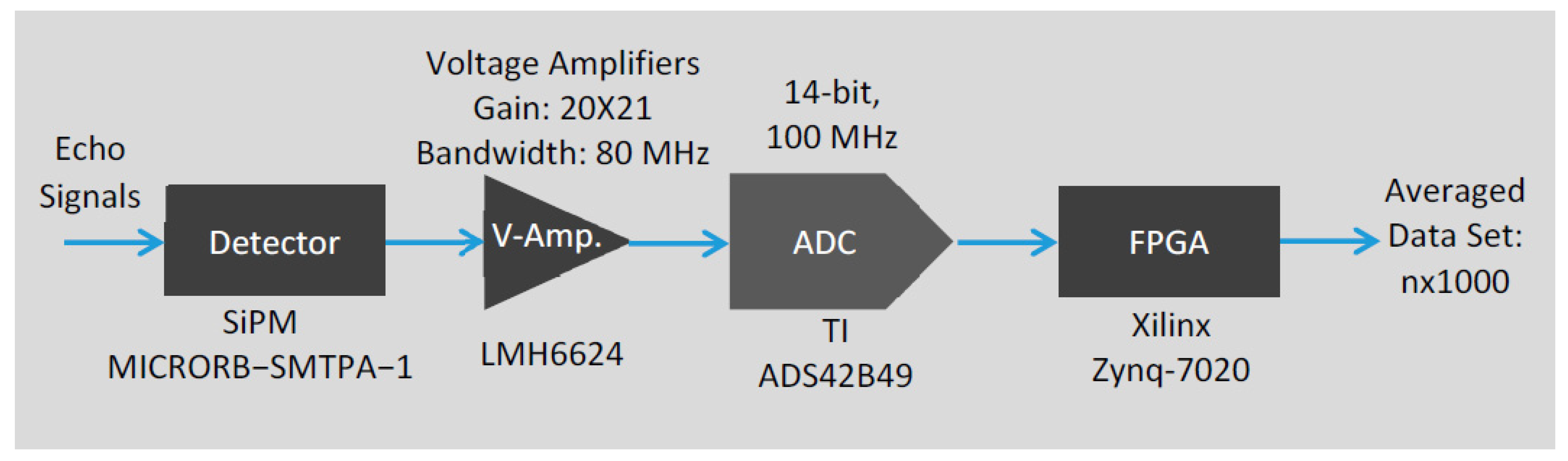
The data acquisition part of our prototype was configured as shown in the block diagram below,
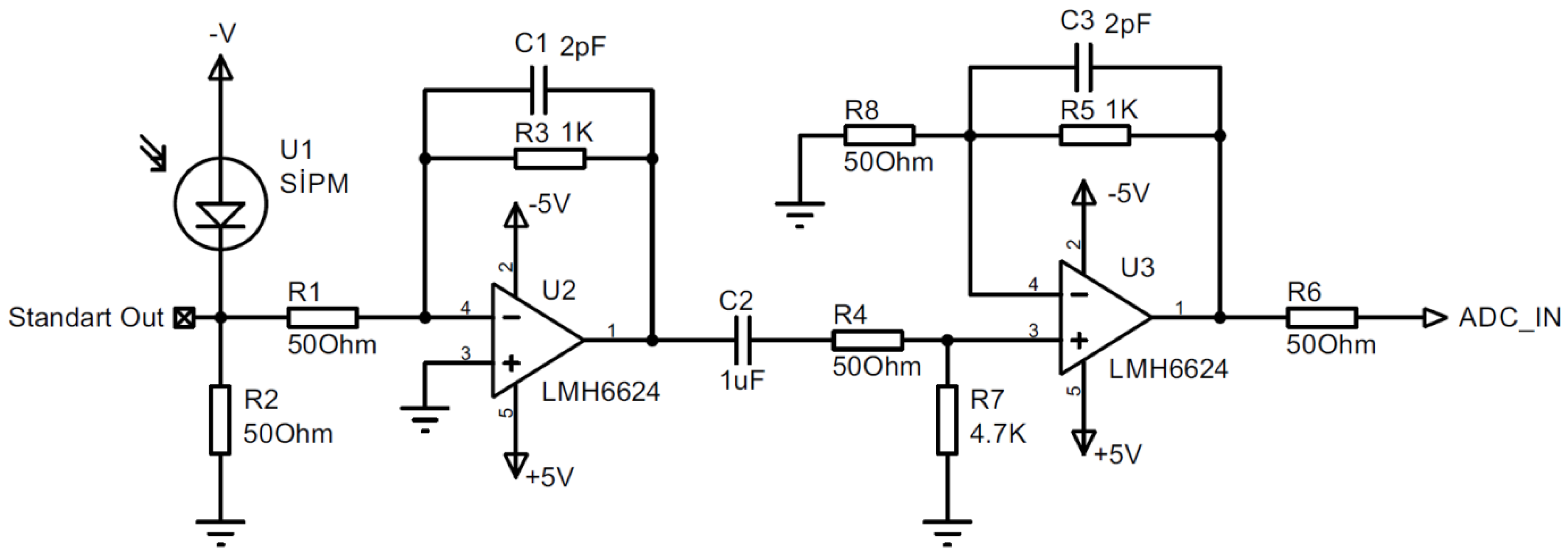
Figure 3. First, analog electrical signals from the photodetector were amplified by the 2-stage voltage amplifier whose circuit diagram is also shown in the
Figure 4. The gain of the amplifier was calculated as 420.
When detecting low power optical signals, amplification of the standard output with band pass filtering was required to provide sufficient gain. To read out the SiPM from the standard output, the photocurrent generated on the detection of photons was first converted to the voltage by 50 Ω load resistor and then is amplified by using a voltage amplifier as depicted in
Figure 4. LMH6624 is ultra-low noise op-amp with 1.5 GHz gain bandwidth product. The cut off frequency of the amplifier circuit was designed to be at 80 MHz as to be compatible with the pulse width for the maximum gain of approximately 420. The amplified and filtered signal was then fed into the high-speed ADC module (ADS42B49, Texas Instruments). It converted analog voltage to 14 bit parallel discrete digital data at a 100 MHz sampling rate. An FPGA module acquired the digital data and transferred the average of 1000 frames at 1 Hz to the computer via a USB port, continuously. Averaging processes were performed by summing each frame point by point and then divided by the total number of frames. Each frame had 4096 sampled data points with a corresponding data point interval of 10 ns. A signal extraction algorithm was developed in Labview platform, running in the computer. Second averaging was done in the algorithm. The number of averaging frame was selected by the user.
3. Signal Extraction Algorithms
There are many noise reduction and signal extraction approaches reported in the literature. Signal accumulation technique [
36] based on the assumption of zero mean random noise is widely used for noise reduction Coherent averaging, constant false alarm rate, wavelet and adaptive filters are also the most common methods. Since the signal is embedded in noise, coherent averaging has to be applied to obtain a meaningful signal [
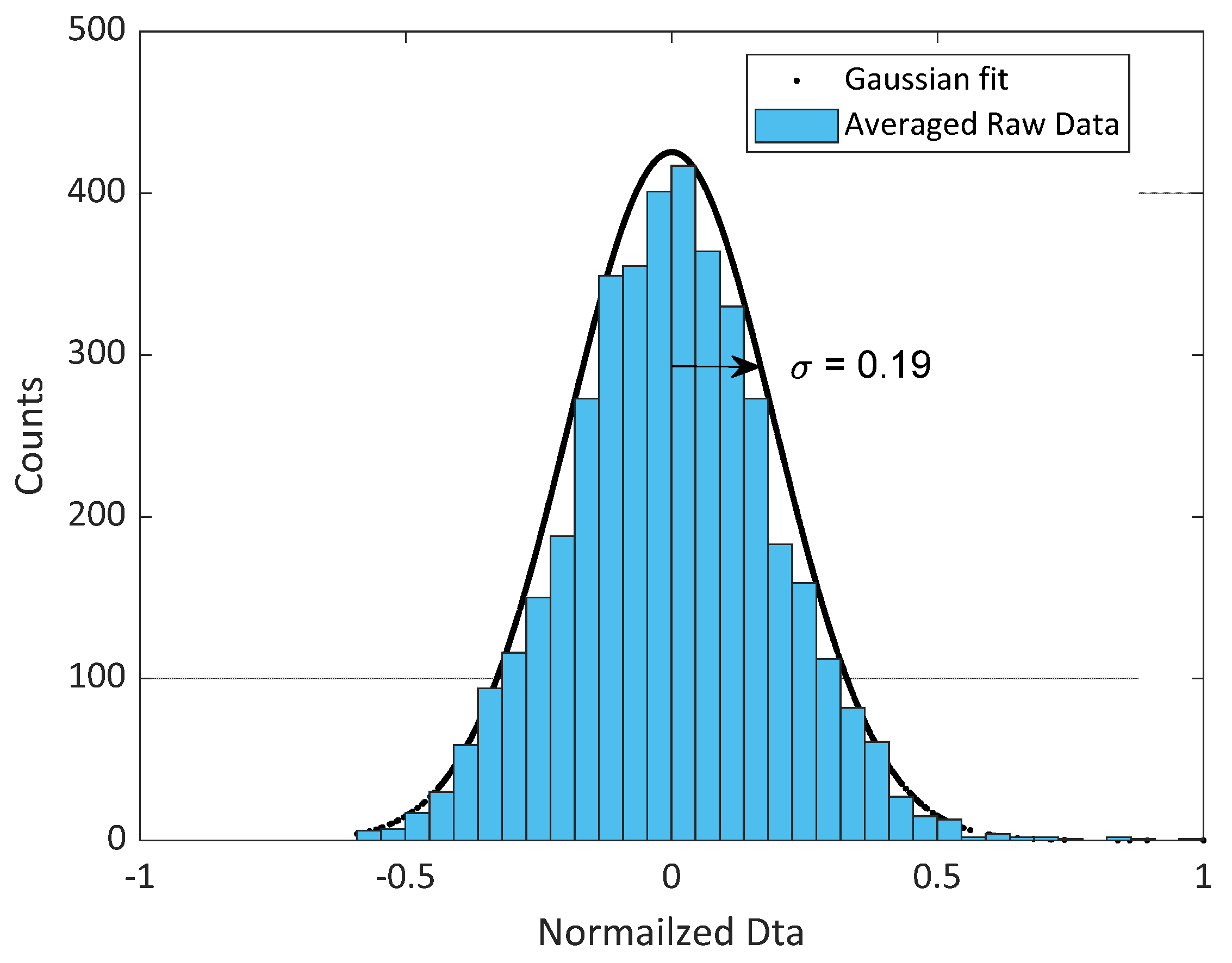
18]. When the laser power is very low, averaging should be done in multiples of 1000 depending on the distance. During the outdoor testing, the performance of our LRF, it has been observed that averaging process of up to 5000 frames is beneficial for noise reduction. At this level, the averaging process can be seen in
Figure 5, where the noisy signal provides a Gaussian distribution.
This situation provides flexibility in determining our signal extraction method. Since the averaging process takes a long time (1 s is required for 1000 frames), signal extraction should be started as soon as the data are acquired. The shape and pulse width of the detected pulse varies depending on the distance and attenuation rate. In addition, the detected signals are accompanied by the noises of all kind which can be classified into two different sources, optical such as background IR radiation, and electronic such as the noise of amplifiers. The SiPM itself also contributes to noise by means of dark current and excess noise. In the near-IR the excess noise of SiPMs appreciably increases even with low background noise [
37]. For this reason, the use of the statistical method was preferred.
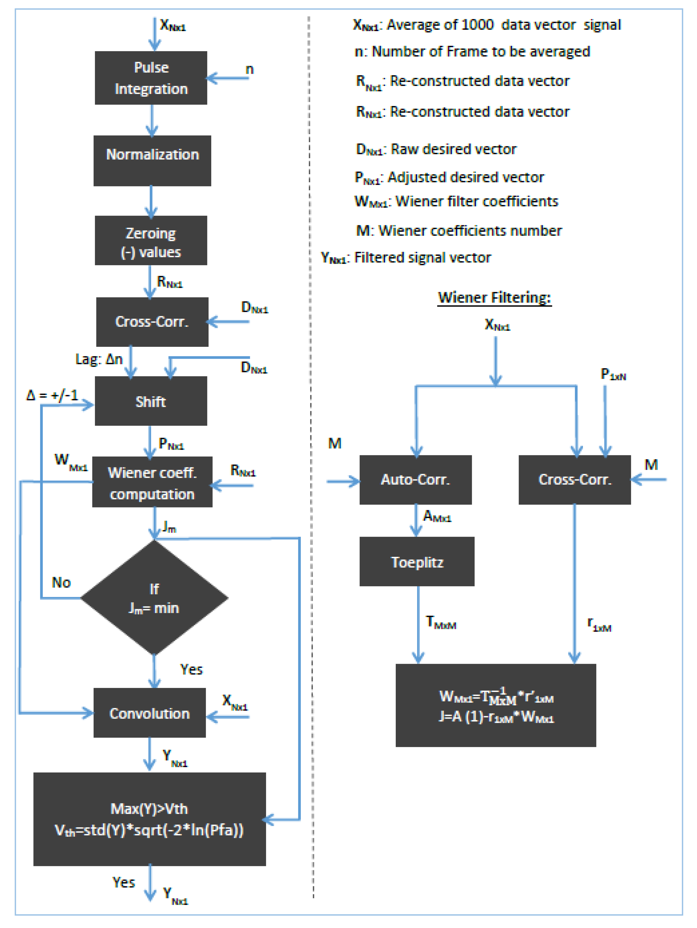
The Wiener-Hopf filter is the most popular statistical-based adaptive filter [
38].
Figure 6 shows the basic outline of this filter which consists of averaging process, determining Wiener-Hopf filter coefficients according to the appearance of noise signal, filtering and the decision steps. The most challenging stage in Wiener filter application is determining the desired signal. In the averaging stage, coherent pulse integration was performed over the measured data signal (shown as X
Nx1) which comes as an average of 1000 data. Here, we can choose any integer number to be averaged so, e.g., if we choose 5, we obtain data which is the average of the 5000 data frame. After normalization and zeroing the negative values, the signal (shown as R
Nx1) enters the Wiener-Hopf process. Using the Wiener-Hopf equation, it is possible to extract the Wiener coefficients according to our desired signal (D
Nx1) properties such as their shapes and positions from the noisy signal. The designed low-pass filter with these coefficients specifically belongs to both the noisy signal and desired signal. Therefore, these coefficients (W
Nx1) need to be recomputed after each measurement. The number of coefficients (M) is also of great importance in terms of computational time and effectiveness of the filtering, as well. Therefore, they need to be optimized and this is done by trial and error.
The data acquired (XNx1) contains 4096 points and data interval corresponds to 10 ns duration. This corresponds to the maximum distance that can be measured is 6144 m. DNx1 is the filtered-out desired signal vector that contains 4096 data points. It is actually defined as all zero except the pulse representing the signal which is composed of 12 data point corresponding to 120 ns when SNR is larger than 3.5. Naturally, this gives an uncertainty in the position of the target which is 18 m. This single desired pulse is the analogy of laser pulse and approximately normalized Gaussian.
The next step is to find the position of the pulse. The position of the pulse in the desired signal is determined by the cross correlation of the designed desired signal at the beginning with acquired noisy signal. This position depends on the SNR of a noisy signal and is not a final position yet. The form of that desired signal is roughly defined as the corrected desired signal. At this stage, Wiener filtering is ready to use for processing roughly corrected desired signal with the acquired noisy signal. The Wiener-Hopf equation written below depends on the cross-correlation of the noisy signal with the desired signal and auto-correlation of noisy signal. As a result of this equation, we obtain number of fifty different filter coefficients. During this process the mean square error (MSE), which shows the degree of success, can be found using these computed coefficients. MSE (shown as Jm in the algorithm) changes between 0 which corresponds to the best result and 1 corresponding to the worst case. After the first computed MSE, we search for 0 or lowest MSE value by sliding the beginning of the roughly corrected desired signal pulse one by one. This search continues both ways until we find the best MSE. In the code, the number of sliding is 200 both ways which is usually enough to find the best MSE. Now, we reconstruct the desired signal with the new one according to the search result. Then we obtain new 50 filter coefficients with these reconstructed desired signals and acquired noisy signals using Wiener-Hopf processing.
In the third stage, filtering is performed by convolving noisy signal with computed filter coefficients. After that the top of the filtered signal (Y
Nx1) can be used to find the position of the target.
Figure 7 shows the success of this algorithm and it was explained in detail as below.
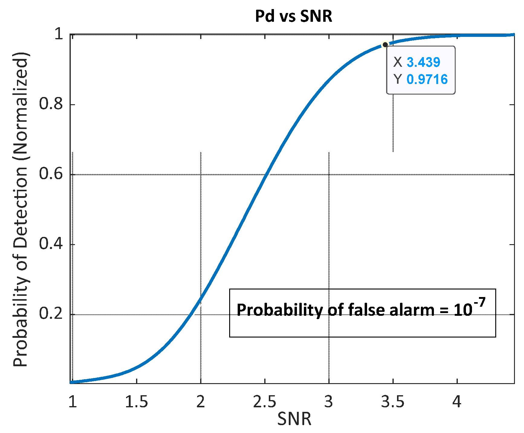
In order to test the power of the algorithm above which is based on the Wiener-Hopf method, we run a Monte Carlo simulation and it is explained as follows. First, we generate Gaussian random noise signal with 4096 data point as to be compatible with an experimentally acquired signal. As known, the SNR of that noise is inversely proportional to the logarithmic of the variance of that signal. Therefore, we generate a noise signal whose SNR in linear scale (not dB) runs from 0 to 4.5 with an interval of 0.5, then interpolation is performed to obtain
Figure 7. Here, we generate 1000 random different noise signals for each SNR value. For instance, we have 1000 different noise signal with an SNR of 3 (in linear scale). Second, we put a deformed square like signal representing the returning pulse somewhere inside the 4096 data point. The place of this artificially created signal in the data actually corresponds to the distance of 2000 m. Here, we have an artificial data signal which contains signal and noise with a known SNR. Next, this signal (X
Nx1 in
Figure 5) goes into the algorithm. After the algorithm runs with this signal, the place of the filtered signal can be determined. Finally, threshold level based on the chosen probability of false alarm (Pfa = 10
−7) can be easily calculated by the computed standard deviation of the filtered signal as given in the equation below [
39].
. The distance can be determined by comparing the signal level with the threshold if the signal height is larger than the threshold. If the computed distance is correct with our previously defined distance, then this corresponds to the true case or wrong case if otherwise. In the case that the signal height is smaller than the threshold, this can be evaluated as a missed case. The
Figure 7 shows the simulation result in terms of how effectively the algorithm runs. For instance, if the SNR is above 3 (linear, not dB), the probability of finding the true distance is 90%. This algorithm is implemented in our real experimental data to find the target distance, and they are shown in
Figure 8,
Figure 9 and
Figure 10.
4. Results and Discussion
The test environment was barren land and tests were conducted on a clear day with mild winds. To view the targets in a wide perspective, the device was positioned on a higher hill than the targets’ positions. We pointed our LRF to three different targets at different distances. As reference, those distances were measured with a commercial long distance LRF of 1064 nm laser with 8 mj energy and resolution of ±5 m.
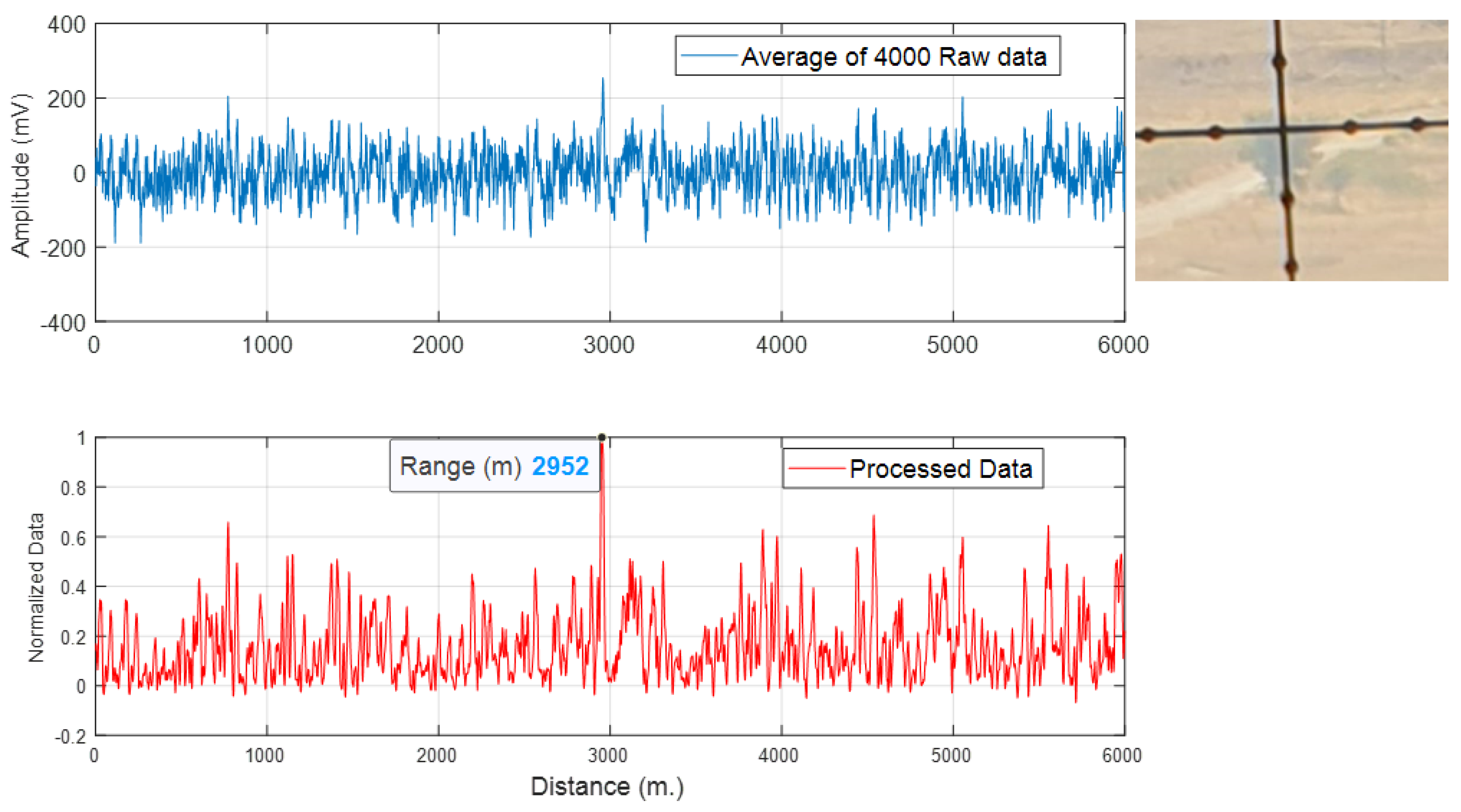
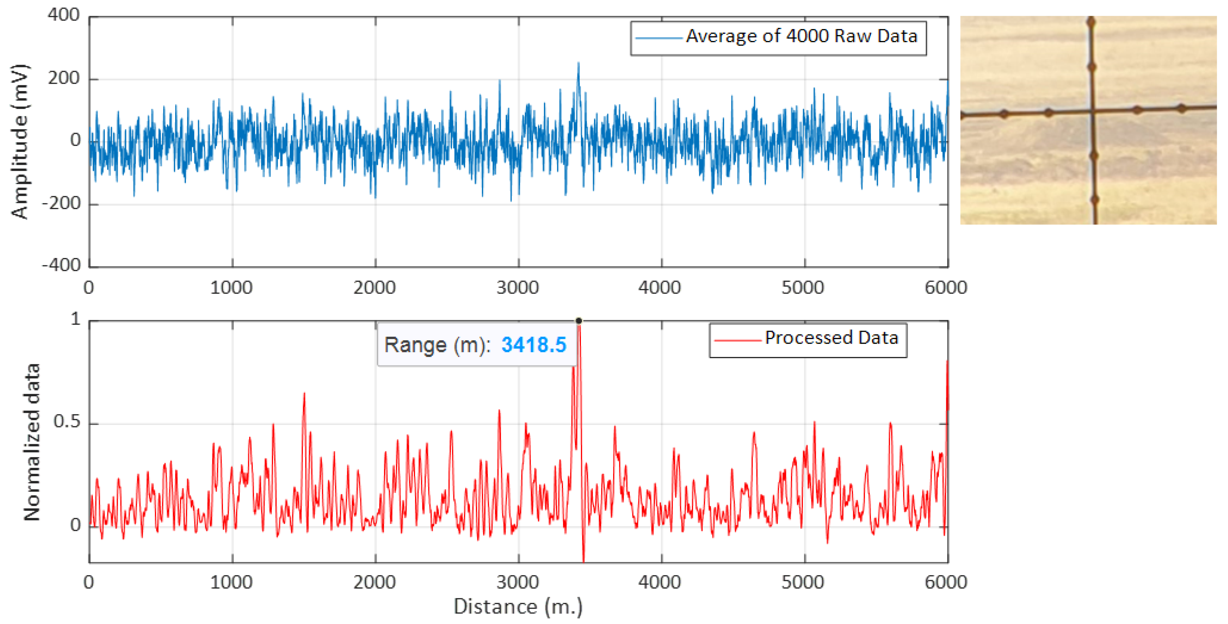
Figure 8,
Figure 9 and
Figure 10 show the average of raw data and the processed data which was obtained with our LRF with a picture of the target taken with a monocular mounted on the top of our LRF (see the
Figure 2).
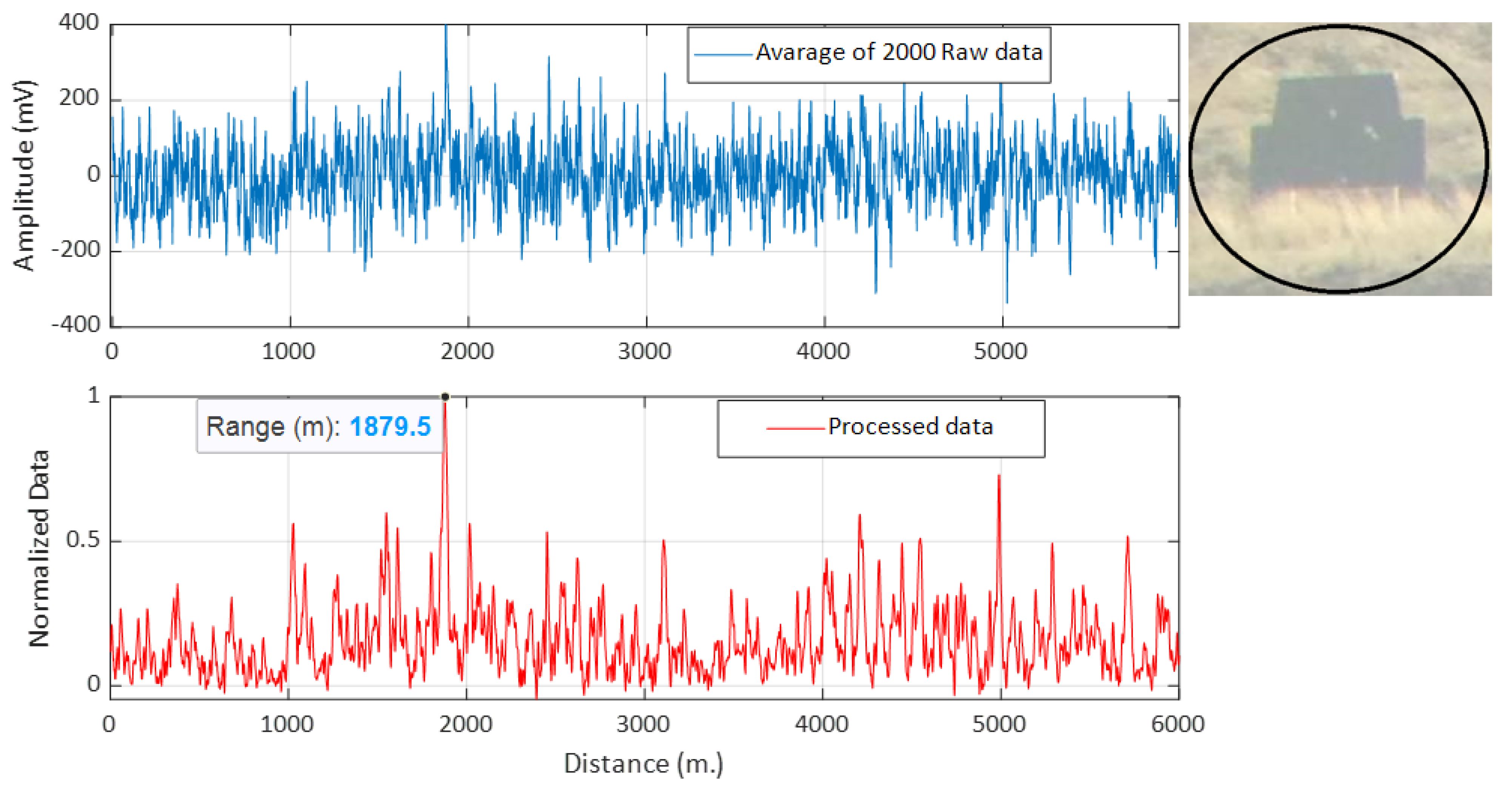
Figure 8 shows the first target which has the size of 2 by 2 m of a black painted wooden plane and measured distance is 1840 m. The second target in
Figure 9 is a solitary tree in the barren land and measured distance is 2940 m. Our third target in
Figure 10 is the small hill in the ground with measured distance of 3385 m. Those distances are measured with our reference laser rangefinder. Blue colors are the averaged raw data and the red colors are the processed data of the blue one using the algorithm shown in
Figure 5. Although any number of averaging could be chosen, the number of averaged data in
Figure 8 is 2000 and in
Figure 9 and
Figure 10 is 4000.
For all cases, IFOV corresponding to those distances and the size of the laser spot are larger than the size of the target. This causes reduced SNR due to incoming unwanted radiation.
As the averaging increases, signal becomes more visible as the SNR increases with square root of N. Calculated SNR of raw data for
Figure 8,
Figure 9 and
Figure 10 are 3.7 dB, 4.2 dB and 4.3 dB, respectively, then after signal processing, SNRs become 7.7, 7.3 and 7.7 decibels, respectively. Using the Wiener filtering algorithm, 3 dB enhancement in SNR for
Figure 8 and 2.5 dB enhancement in SNR for other figures are obtained. Our LRF data after the algorithm correctly found the position of the signal with an average error of approximately 30 m. This can be due to the delay which can be corrected by the proper calibration.


