Optimizing Automatic Transmission Double-Transition Shift Process Based on Multi-Objective Genetic Algorithm

Abstract

In order to improve fuel economy, the number of gears in the hydraulic automatic transmission of heavy-duty mining trucks is continuously increasing. Compared with single-transition shifts, double-transition shifts can optimize the structure of multi-speed transmissions, but the difficulty of control will also increase. In this paper, a dynamic model of a 6 + 2 speed automatic transmission and vehicle powertrain system are built based on the Lagrange method, and the dynamic analysis of the two sets of clutches that make up the double-transition shift are carried out. Since a simulation model of the double-transition shift process is built-in MATLAB/Simulink, the shift jerk and clutch energy loss are used as multi-objective, and the genetic algorithm is used to optimize the simulation. Five strategies for the overlapping time of the clutches are proposed, and simulation experiments and Pareto optimal analysis are carried out, respectively. The simulation results show that the non-overlapping of the two sets of clutch inertia phases in the double-transition shift can effectively reduce the shift jerk. The overlapping of the torque phase and the inertia phase of the other clutch set can control the clutch energy loss at a low level due to using less shift time.

1. Introduction

Since the need for the market and regulations to improve the fuel economy and smoothness of heavy-duty mining trucks, increasing the number of the forward gears is the trend of developing the new high-power hydraulic automatic transmission (AT) [1,2,3]. The single-transition shift (STS, that is, one clutch is going to engage while the other clutch needs to be disengaged) can no longer meet the designing requirements of a higher number of gears and more reasonable gear ratio distribution within a limited space [4]. Double-transition shift (DTS) is a dual single-transition shift process, which requires multiple clutches (typically four) for precisely coordinated control. If any clutch is not precisely controlled, power interruption or conflict may happen, and the shift quality will deteriorate [5,6]. The DTS involving more clutch elements is more complicated than the STS of traditional transmission, which poses a higher challenge to the AT control system of heavy-duty mining trucks [7].

In order to improve the AT shift quality, the researchers used different modeling and optimization methods to study the clutch-to-clutch control system [8,9,10,11,12]. Ranogajec et al. [13,14] used the bond graph method to analyze the dynamics of a shift process for a ten-speed automatic transmission, and they proposed a solution by using an extra clutch to compensate the output torque, so as to assist the gear shift and suppress the excessive impact of the inertial phase. Zhao and Li [15] adopted subspace identification to describe the predictive equations of single-transition shift and then used the model predictive control method to optimize the shifting quality. In the research of the nonlinear dynamic characteristics of the wet clutch, a clutch pressure controller based on sliding mode control was designed to ensure a smooth clutch-to-clutch shift by Song and Sun [16]. Meng et al. [17] focused on the analysis of an AT electro-hydraulic control system and proposed a two-degree-of-freedom proportional-integral-derivative control optimization method to ensure that the clutch relative speed difference follows the preset trajectory curve by adjusting the proportional solenoid valve duty cycle. To achieve the balance among the sportiness, comfort, and robustness during the shift, the multi-objective genetic algorithm was used to get Pareto-optimal frontier by Wurm and Bestle [18].

Compared with the aforementioned large amount of literature on STS, there are few studies on the double-transition shift. Wu and Hebbale [19,20] established a DTS model based on the theory of multi-body dynamics, analyzed the motion state of the components, and proposed a parameter-based control strategy. Ivanović et al. [6,21] studied DTS power downshifts (10-6 gears) and proposed six different additional constraint schemes of clutch torque and speed during shift transients. Through simulation analysis, the simulation results show that the rapid pressure reduction of the two clutches to be disconnected is the optimal control scheme, but the article lacks the research on the overlap time of the two clutch sets.

Therefore, in terms of the AT equipped on heavy-duty mining trucks with DTS, this paper uses the Lagrange method to build the dynamic model of the high-power transmission and the vehicle powertrain system at first. Secondly, the dynamic analysis of the DTS, which is composed of a group of the STS power upshift and a group of downshift, is carried out. Then, five strategies for the overlap time of the two sets of clutches in the DTS are proposed. After the multi-objective genetic algorithm optimization is performed with the shift jerk and the clutch friction loss as the performance indicators, the Pareto optimal result analysis and simulation are performed. Finally, conclusions are drawn.

2. Modeling of DTS

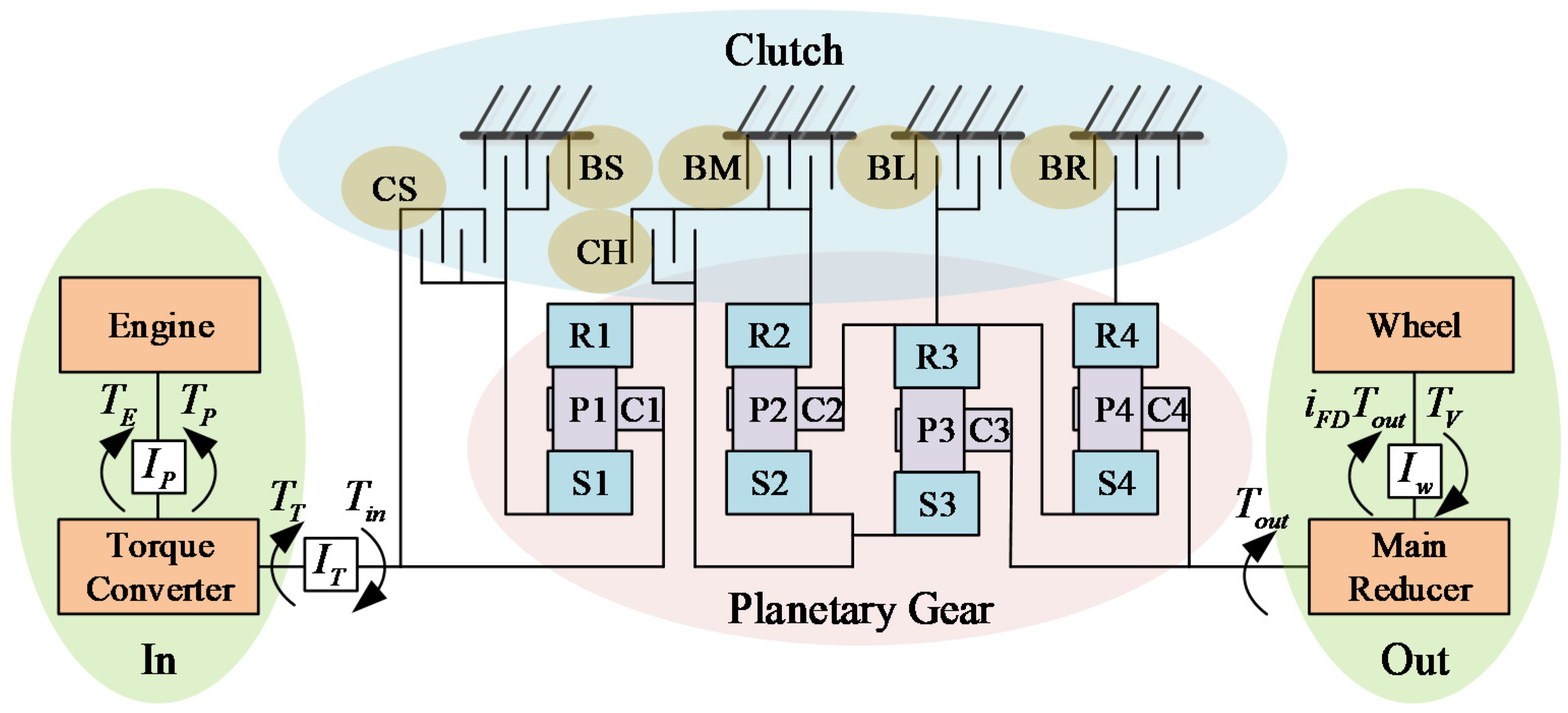
As shown in Figure 1, the AT powertrain system in this paper can be divided into the planetary gear sets model, the clutch pressure control model, the transmission power input model (composed of diesel engine and torque converter), and the power output model (drive axle and vehicle longitudinal dynamics model).

2.1. Modeling of the Planetary Gear Sets Based on the Lagrange Method

Instead of traditional dynamics analysis, the bond graph method, and lever analogy, the Lagrange method does not need to consider the actual gear structure and calculate the interaction force and torque on each element [15,22], so it is a good way to solve complex dynamic equations of planetary gear sets in DTS.

A high-power 6 + 2-speed AT is composed of four planetary gear sets—where $Si$, $Ri$, $Ci$, and $Pi$ respectively represent the sun gear, ring gear, planet carrier, and planetary gear ($i=1, 2, 3, 4$)—and six electro-hydraulic actuated clutches ($CS$, $BS$, $CH$, $BM$, $BL$, and $BR$). The combined clutch/brake schedule is shown in

Table 1. Combined clutch/brake schedule.

Gears	CS	BS	CH	BM	BL	BR	Gear Ratio
1	√				√		4.00
2		√			√		2.67
3	√			√			2.00
4		√		√			1.33
5	√		√				1.00
6		√	√				0.67
R1	√					√	−5.00
R2		√				√	−3.33

. The fourth planetary set and the clutch $BR$ are ignored in the following modeling because they only participate in reverse gear.

Based on the velocity relationship of a mesh point, the kinematics equations of each planetary set are

$$\{\begin{array}{l}{\omega }_{Ci}{R}_{Si}-{\omega }_{Pi}{R}_{Pi}={\omega }_{Si}{R}_{Si}\\ {\omega }_{Ci}\left(R_{Si}+2R_{Pi}\right)+{\omega }_{Pi}{R}_{Pi}={\omega }_{Ri}{R}_{Ri}\end{array},$$

(1)

where $\omega$ is the angular velocity of the component and $R$ is the radius. Therefore, the planetary gear system has six constraint equations and nine motion parameters, and the system is a three-degree-of-freedom system. ${\omega }_{S1}$, ${\omega }_{C1}$, and ${\omega }_{C3}$ are selected as independent variables to facilitate calculation, and other coordinate parameters can be expressed by these three independent variables as

$${\left[\begin{array}{cccccc}{\omega }_{R1S2S3}& {\omega }_{C2R3}& {\omega }_{R2}& {\omega }_{P1}& {\omega }_{P2}& {\omega }_{P3}\end{array}\right]}^T=A{\left[\begin{array}{ccc}{\omega }_{S1}& {\omega }_{C1}& {\omega }_{C3}\end{array}\right]}^T,$$

(2)

where $A$ is the constant coefficient matrix determined by the transmission structure. Since the planetary gears are symmetrically arranged, the potential energy change is considered to be zero $E_p=0$. Thus, the total energy of the system $E$ can be regarded as the sum of the kinetic energy $E_k$.

$$E=E_p+E_k=E_k,$$

(3)

Each component kinetic energy $\kappa$ can be expressed as

$$E_k={\displaystyle \sum _{i=1}^3{\kappa }_{Si,Ci,Ri,Pi}}={\displaystyle \sum _{i=1}^3\frac{1}{2}{I}_{Si,Ci,Ri,Pi}{\omega }_{Si,Ci,Ri,Pi}^2}=E_k\left(\begin{array}{ccc}{\omega }_{S1}& {\omega }_{C1}& {\omega }_{C3}\end{array}\right),$$

(4)

where $I$ is the rotational inertia. The Lagrange equation of the system is written as

$$\{\begin{array}{l}{Q}_{S1}=\frac{d}{dt}\left(\frac{\partial E}{\partial {\omega }_{S1}}\right)-\frac{\partial E}{\partial {\alpha }_{S1}}\\ Q_{C1}=\frac{d}{dt}\left(\frac{\partial E}{\partial {\omega }_{C1}}\right)-\frac{\partial E}{\partial {\alpha }_{C1}}\\ Q_{C3}=\frac{d}{dt}\left(\frac{\partial E}{\partial {\omega }_{C3}}\right)-\frac{\partial E}{\partial {\alpha }_{C3}}\end{array},$$

(5)

where $Q$ is the generalized torque of the system on independent variables. According to the principle of virtual work, the virtual work of the system $\delta W$ is the sum of the products of the virtual angular displacement $\delta \alpha$ and each component torque $T$.

$$\delta W={\displaystyle \sum _{i=1}^3{T}_{Si,Ci,Ri,Pi}\delta {\alpha }_{Si,Ci,Ri,Pi}}$$

(6)

Based on the connection relationship between the clutch and each component from Figure 1, it can be summarized as

$$\begin{array}{cc}\hfill \delta W& =\left(T_{f,CS}+T_{f,BS}+A_{11}{T}_{f,CH}-A_{31}{T}_{f,CS}+A_{31}{T}_{f,BM}+A_{21}{T}_{f,BL}\right)\delta {\alpha }_{S1}\hfill \\ & +\left(T_{in}-T_{f,CS}+A_{12}{T}_{f,CH}-A_{32}{T}_{f,CH}+A_{32}{T}_{f,BM}+A_{22}{T}_{f,BL}\right)\delta {\alpha }_{C1}\hfill \\ & +\left(A_{13}{T}_{f,CH}-A_{33}{T}_{f,CH}+A_{33}{T}_{f,BM}+A_{23}{T}_{f,BL}-T_{out}\right)\delta {\alpha }_{C3}\hfill \end{array}.$$

(7)

From Equation (7), $Q$ can be derivate as

$$\{\begin{array}{l}{Q}_{S1}=T_{f,CS}+T_{f,BS}+A_{11}{T}_{f,CH}-A_{31}{T}_{f,CS}+A_{31}{T}_{f,BM}+A_{21}{T}_{f,BL}\\ Q_{C1}=T_{in}-T_{f,CS}+A_{12}{T}_{f,CH}-A_{32}{T}_{f,CH}+A_{32}{T}_{f,BM}+A_{22}{T}_{f,BL}\\ Q_{C3}=A_{13}{T}_{f,CH}-A_{33}{T}_{f,CH}+A_{33}{T}_{f,BM}+A_{23}{T}_{f,BL}-T_{out}\end{array}.$$

(8)

Introducing Equations (4) and (8) into Equation (5), the dynamic equations of the planetary gear sets on the independent variables can be obtained

$$D{\left[\begin{array}{ccc}{\dot{\omega }}_{S1}& {\dot{\omega }}_{C1}& {\dot{\omega }}_{C3}\end{array}\right]}^T=B{\left[\begin{array}{ccccccc}{T}_{in}& T_{f,CS}& T_{f,BS}& T_{f,CH}& T_{f,BM}& T_{f,BL}& T_{out}\end{array}\right]}^T,$$

(9)

where $D$ is a rotational inertia matrix, and $B$ is a constant coefficient matrix composed of $A$.

According to Equation (2), the angular acceleration relationship of the component can be re-written as

$${\left[\begin{array}{ccc}{\dot{\omega }}_{R1S2S3}& {\dot{\omega }}_{C2R3}& {\dot{\omega }}_{R2}\end{array}\right]}^T=H{\left[\begin{array}{ccc}{\dot{\omega }}_{S1}& {\dot{\omega }}_{C1}& {\dot{\omega }}_{C3}\end{array}\right]}^T,$$

(10)

where $H$ is a constant coefficient matrix composed of $A$. The relationship between the clutch relative speed $\Delta \omega$ and the rotation speed of each component is

$$\left[\begin{array}{c}\Delta {\dot{\omega }}_{CS}\\ \Delta {\dot{\omega }}_{BS}\\ \Delta {\dot{\omega }}_{CH}\\ \Delta {\dot{\omega }}_{BM}\\ \Delta {\dot{\omega }}_{BL}\end{array}\right]=\left[\begin{array}{c}{\dot{\omega }}_{C1}-{\dot{\omega }}_{S1}\\ -{\dot{\omega }}_{S1}\\ {\dot{\omega }}_{R2}-{\dot{\omega }}_{R1S2S3}\\ -{\dot{\omega }}_{R2}\\ {\dot{\omega }}_{C2R3}\end{array}\right]=K\left[\begin{array}{c}{\dot{\omega }}_{S1}\\ {\dot{\omega }}_{C1}\\ {\dot{\omega }}_{C3}\\ {\dot{\omega }}_{R1S2S3}\\ {\dot{\omega }}_{C2R3}\\ {\dot{\omega }}_{R2}\end{array}\right].$$

(11)

Therefore, the dynamic equation of the planetary gear sets system can be obtained by combining Equations (9)–(11).

$$\left[\begin{array}{c}\Delta {\dot{\omega }}_{CS}\\ \Delta {\dot{\omega }}_{BS}\\ \Delta {\dot{\omega }}_{CH}\\ \Delta {\dot{\omega }}_{BM}\\ \Delta {\dot{\omega }}_{BL}\end{array}\right]=K\left[\begin{array}{c}{D}^{-1}B\\ H{D}^{-1}B\end{array}\right]\left[\begin{array}{c}{T}_{in}\\ T_{f,CS}\\ T_{f,BS}\\ T_{f,CH}\\ T_{f,BM}\\ T_{f,BL}\\ T_{out}\end{array}\right]=M\left[\begin{array}{c}{T}_{in}\\ T_{f,CS}\\ T_{f,BS}\\ T_{f,CH}\\ T_{f,BM}\\ T_{f,BL}\\ T_{out}\end{array}\right], \mathrm{where}M=\left[\begin{array}{ccccccc}-5.2& 18.2& 13.4& -5.0& -1.1& 0.5& -1.4\\ -9.4& 23.4& 32.7& -3.0& -0.7& 0.3& -0.8\\ -2.0& -5.0& -3.0& 7.7& 3.2& 0.6& 0.7\\ 0.5& 1.1& 0.7& -3.2& -2.2& -1.1& 0.6\\ -0.2& -0.5& -0.3& -0.6& -1.1& -0.9& 0.8\end{array}\right]$$

(12)

2.2. Modeling of Clutch Friction

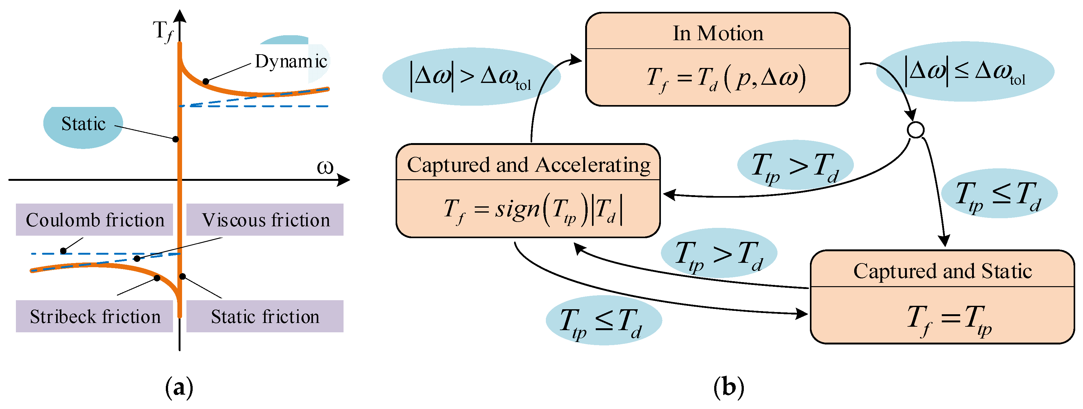
The Stribeck friction model, as shown in Figure 2a, is used to describe the dynamics of the clutch friction pair.

$$T_d=sign\left(\Delta \omega \right)f(\Delta \omega )S_{C}RNp,$$

(13)

where $f(\Delta \omega )=0.06+0.04e^{(-0.36\Delta \omega )}$ is the friction factor for a copper-based surface, $S_C$, $R$, $N$, and $p$ are the equivalent area, the equivalent radius, the friction pairs number, and the pressure of clutch, respectively, $T_{tp}$ is the required torque, and $△{\omega }_{tol}$ is the threshold of the clutch relative speed. According to the difference in the relative speed of the clutch plate and the friction plate, and the difference in the transmission torque capacity and the required torque, the clutch friction working mode switches among “in motion”, “captured and accelerating”, and “captured and static”, as shown as Figure 2b [23].

2.3. Modeling of the Transmission Input Power

The co-working output characteristics of the diesel engine and the torque converter (TC) determine the input power of the transmission. The output torque of the diesel engine $T_E$ is related to its rotational speed ${\omega }_E$ and throttle opening $\theta$.

$$T_E\left({\omega }_E,\theta \right)=T_P+I_P{\dot{\omega }}_P,$$

(14)

where $T_P$ is the pump torque, $I_P$ is the equivalent inertia of the turbine, and ${\omega }_P$ is the pump speed.

Connected to the engine and the transmission input shaft, the torque converter is composed of the pump, the turbine, and the guide wheel. The dimensionless characteristics of the torque converter (including the pump torque coefficient ${\lambda }_P$, the TC torque ratio $K_{TC}$, speed ratio $i_{TC}$, and efficiency ${\eta }_{TC}$) are used to describe their dynamic equation given by [24]

$$\{\begin{array}{c}{T}_P={\lambda }_P{\rho }_{TC}g{D}_{TC}{}^5{\omega }_P^2\\ T_T=K_{TC}{T}_P\\ {\omega }_T=i_{TC}{\omega }_P\\ P_T=T_T{\omega }_T={\eta }_{TC}{P}_P=K_{TC}{i}_{TC}{T}_P{\omega }_P\end{array},$$

(15)

where ${\rho }_{TC}$ is the fluid density of the torque converter, $D_{TC}$ is the effective diameter of the torque converter, $T_T$ is the turbine torque, ${\omega }_T$ is the turbine speed, and $P_T$ and $P_P$ are the power of the turbine and pump.

2.4. Modeling of the Transmission Output Power

The torque output by the AT transmission is finally transmitted to the wheels through the main reducer (speed ratio $i_{FD}$). For modeling convenience, the longitudinal vehicle model was simplified, without considering the vehicle’s pitch, yaw, and other motion directions. The AT output torque is described as

$$T_{out}=\frac{I_w{\dot{\omega }}_w+T_V}{i_{FD}},$$

(16)

where ${\omega }_w$ is the wheel speed and $I_w$ is the equivalent inertia of wheels. When the heavy-duty mining truck is under non-braking condition, the vehicle longitudinal resistance torque $T_V$ can be described by

$$T_V=r_w\left(Mg{f}_{\mathrm{roll}}+\frac{C_D{S}_V}{21.15}{v}_V{}^2+Mg\sin \alpha \right),$$

(17)

where $r_w$ is the radius of the wheel, $M$ is the full load mass, $f_{roll}$ is the rolling resistance coefficient, $C_D$ is the air resistance coefficient, $S_V$ is the windward area,, $v_V$ is the vehicle speed, and $\alpha$ is the road slope, respectively.

3. Double-Transition Shift Process Analysis

As shown in Table 1, 2–3, 4–5 upshifts, and 3–2, 5–4 downshifts are double-transition shifted. In this paper, we take 2–3 upshift as an example. During this shifting process, the two sets of clutches (one set is $BL$ and $BM$, another set is $BS$ and $CS$) act at the same time, where the clutch $BS$ and $BL$ are disengaged, $CS$ and $BM$ are engaged gradually, and the state of $CH$ does not change. The shifting process of these two sets of clutches will be analyzed separately below.

3.1. BL and BM Power on Upshift Process Analysis

In the first set of clutches, $BL$ as the off-going clutch (OFC) and $BM$ as the on-coming clutch (ONC) undergo a state transition. This can be seen as the 2–4 single-transition upshift and can be divided into four stages, which are low gear phase, torque phase, inertia phase, and high gear phase.

The low gear phase mainly prepares for the upshift to eliminate the gap between the clutch and the oil circuit. In the high gear phase, the oil pressure continues to increase after $BM$ drops to zero speed, so that it has sufficient torque capacity to ensure the clutch in the locked state. There is no torque or speed change in these two stages, and the transmission is in a steady state.

In the torque phase, although the clutch $BL$ starts to drain, the actual torque transmitted at this time is less than the maximum torque determined by static friction force. The clutch is still in the “captured and static” mode $T_{f,BL}=T_{tp,BL}$, and no sliding between the clutch plate ${\omega }_{BL}=0$. At the same time, $BM$ starts oil-filled engagement. As the oil pressure rises, this clutch enters the “in motion” mode and transmits friction torque $T_{f,Bm}=T_{d,Bm}\left(P_{Bm},\Delta {\omega }_{Bm}\right)$. When the maximum static friction torque of $BL$ is less than its actual required torque, sliding begins, and the torque phase ends. At this stage, the dynamic equation is described as

$$\begin{array}{l}0=M_{21}{T}_{in}+M_{23}{T}_{tp,BS}+M_{25}{T}_{d,BM}+M_{26}{T}_{tp,BL}+M_{27}{T}_{out}\\ 0=M_{51}{T}_{in}+M_{53}{T}_{tp,BS}+M_{55}{T}_{d,BM}+M_{56}{T}_{tp,BL}+M_{57}{T}_{out}\end{array}.$$

(18)

At this moment, it is considered that $T_{in}$ and $T_{tp,BS}$ are unchanged. When the amount of change in the torque of $BL$ and $BM$ are the same $\Delta T_{tp,BL}=\Delta T_{d,BM}$, the impact of $BL$ on the output torque is greater than $BM$ because of the coefficient $\left|M_{25}\right|>\left|M_{26}\right|$ in Equation (18). This results in a decrease in the output torque $T_{out}$, which is called the torque hole effect.

In the inertia phase, both $BL$ and $BM$ are sliding in the “in motion” mode $T_{f,BL}=T_{d,BL}\left(P_{BL},\Delta {\omega }_{BL}\right)$, $T_{f,BM}=T_{d,BM}\left(P_{BM},\Delta {\omega }_{BM}\right)$, and ${\omega }_{BL}\ne 0$. In this process, not only the torque changes, but also the rapid changes in the speed and transmission ratio. The inertial effect is enhanced, and the system is in an unstable state. As the oil pressure of $BM$ continues to increase, its relative speed gradually decreases to zero at the end of the inertia phase. In the inertial phase, the dynamic equation is described as

$$\begin{array}{l}\Delta {\dot{\omega }}_{BM}=M_{51}{T}_{in}+M_{53}{T}_{tp,BS}+M_{55}{T}_{d,BM}+M_{56}{T}_{d,BL}+M_{57}{T}_{out}\\ \Delta {\dot{\omega }}_{BL}=M_{61}{T}_{in}+M_{63}{T}_{tp,BS}+M_{65}{T}_{d,BM}+M_{66}{T}_{d,BL}+M_{67}{T}_{out}\end{array}.$$

(19)

While $BL$ has been disconnected and no longer transmits torque $T_{f,BL}=0$, the required torque of $BM$ continues to rise to reduce the input shaft speed to the 4th gear level and lock $BM$. When $BM$ is close to zero speed, it enters the “captured and accelerating” mode $T_{f,BS}=sign\left(T_{tp,BS}\right)\left|T_{d,BS}\right|$. Since the static friction torque is greater than the dynamic friction torque, the output shaft torque rises above the required torque of the fourth gear, which is called the torque bump effect.

3.2. BS and CS Power on Downshift Process Analysis

The state transition of $BS$ and $CS$ can be regarded as a 2–1 single-transition downshift process. Since the direction of power transmission is different from the upshift, the process is divided into a high gear phase, inertia phase, torque phase, and low gear phase in sequence.

The high gear phase is to continuously reduce the $BS$ pressure until it enters the sliding friction state; the low gear phase is to increase the $CS$ pressure to keep it locked after the shift is completed. No changes in the clutch torque or speed have been taken in these two stages, and the transmission is in stable states.

While the $BS$ speed increases from zero, its torque dropped after the inertia phase begins, which led to the transmission output torque continuing to decrease as the friction torque decreases, resulting in the torque hole effect. At here, the output shaft speed is considered to be constant (due to the large load inertia). The increase in the input shaft speed causes the speed of $CS$ to gradually decrease until it reaches zero speed, and the inertia phase ends. According to Equation (12), the inertia phase is described as

$$\begin{array}{l}\Delta {\dot{\omega }}_{CS}=M_{11}{T}_{in}+M_{12}{T}_{d,CS}+M_{13}{T}_{d,BS}+M_{16}{T}_{tp,BL}+M_{17}{T}_{out}\\ \Delta {\dot{\omega }}_{BS}=M_{21}{T}_{in}+M_{22}{T}_{d,CS}+M_{23}{T}_{d,BS}+M_{26}{T}_{tp,BL}+M_{27}{T}_{out}\end{array}.$$

(20)

In the torque phase, the speed ratio alternation is completed, and the angular acceleration of each component tends to zero. Similar to Equation (18), the dynamic equation is described as

$$\begin{array}{l}0=M_{11}{T}_{in}+M_{12}{T}_{tp,CS}+M_{13}{T}_{d,BS}+M_{16}{T}_{tp,BL}+M_{17}{T}_{out}\\ 0=M_{51}{T}_{in}+M_{52}{T}_{tp,CS}+M_{53}{T}_{d,BS}+M_{56}{T}_{tp,BL}+M_{57}{T}_{out}\end{array}.$$

(21)

Due to the coefficient $\left|M_{12}\right|>\left|M_{13}\right|$ in Equation (21), the increase of $CS$ torque occupies a dominant position compared with the effect of the reduction of $BS$ on the output shaft torque, so the output torque exceeds the first gear required torque (the torque bump effect). When the torque drops to zero, all the load torque is borne by $CS$, and the torque phase is completed.

4. Multi-Objective Optimization of DTS

The double-transition shift process not only requires appropriate action between each on-coming and off-going clutches, the reasonable allocation of overlapping time between the two sets of clutches is important as well. In this article, we set the group of $BS$ and $CS$ shift time unchanged, and take the $BL$ and $BM$ shift time as variables. Five control strategies are proposed to sequentially change the overlap time of the two sets of clutches (summarized in

Table 2. Five control strategies for double-transition shift (DTS).

Time	BS and CS	BL and BM
		Strategy 1	Strategy 2	Strategy 3	Strategy 4	Strategy 5
$t_0\sim t_1$		low gear
$t_1\sim t_2$		torque phase	low gear
$t_2\sim t_3$	high gear	inertia phase	torque phase	low gear
$t_3\sim t_4$	inertia phase	high gear	inertia phase	torque phase	low gear
$t_4\sim t_5$	torque phase		high gear	inertia phase	torque phase	low gear
$t_5\sim t_6$	low gear			high gear	inertia phase	torque phase
$t_6\sim t_7$					high gear	inertia phase
$t_7\sim t_8$						high gear

).

The shift jerk $j$ and the clutch friction loss $W$ as the performance indicators of the double-transition shift are a pair of paradoxes. The multi-objective function is

$$\begin{gathered} \min J_1=\frac{1}{p}\sqrt{\frac{1}{t_f-t_0}{\displaystyle {\int }_{t_0}^{t_f}{j}^2}dt}, \\ \min J_2=\frac{r}{q}{\displaystyle {\int }_{t_0}^{t_f}{\displaystyle \sum W}}dt, \end{gathered}$$

(22)

where $r$ is the weight coefficient, and $p=8$ and $q=40,000$ are the normalizing coefficients between the two indicators.

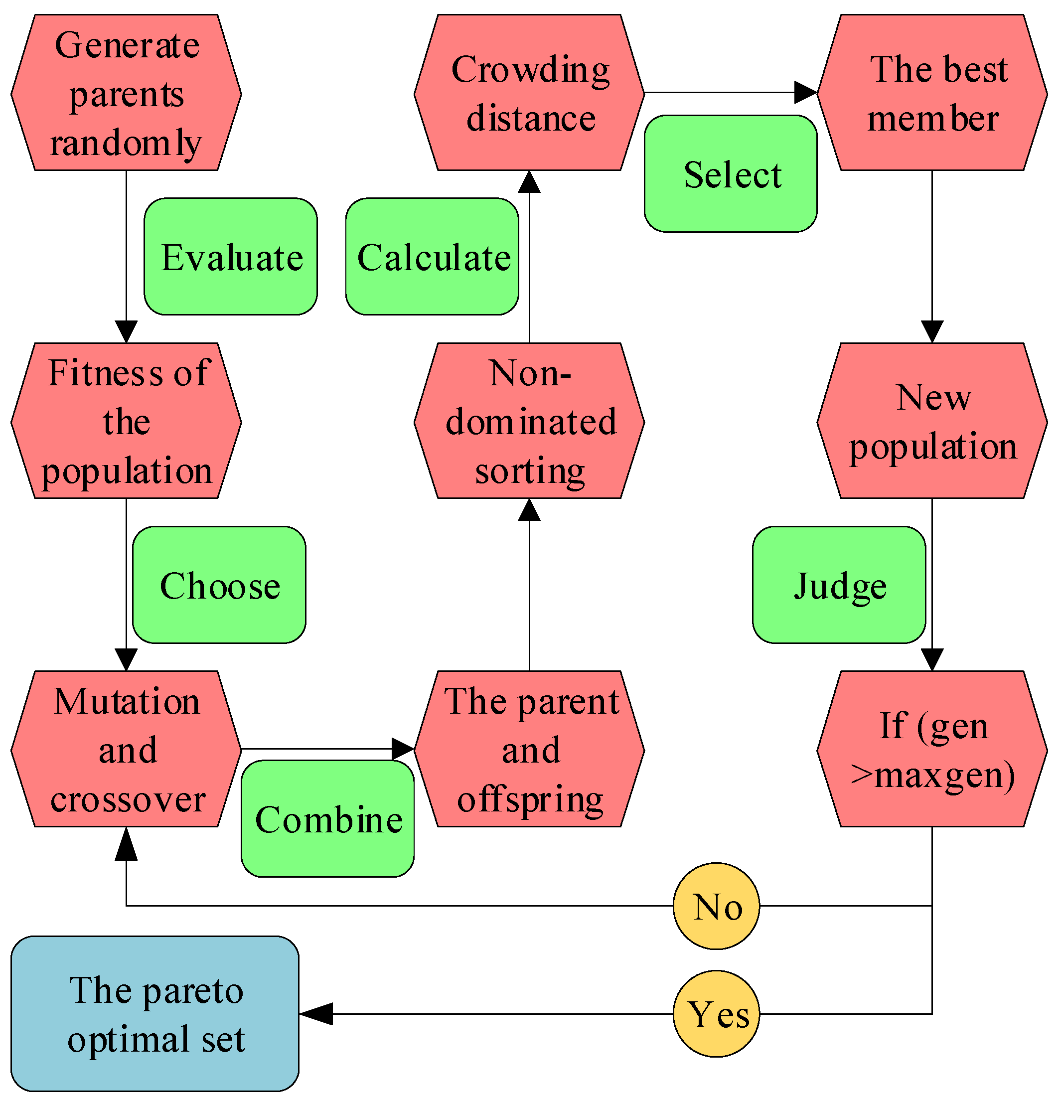
The multi-objective genetic algorithm has been used to optimize a nonlinear problem in the vehicle field [25,26]. Especially, non-dominated sorting genetic algorithm II (NSGA-II) is claimed to have better performance compared with the other optimization methods. A flow diagram of NSGA-II is shown in Figure 3, where all the major steps are shown. A detailed analysis of the algorithm can be found in [27].

In this paper, the optimal front-end individual coefficient is set to 0.3, the population density is set to 20, the maximum number of iterations is 50, and the fitness function deviation is 1e−100. The full-loaded flat road of heavy-duty mining trucks is selected as the simulation condition (vehicle mass $m=72 \mathrm{T}$, road slope $\alpha =0^{°}$); then, it changes the weight coefficient $r$ in turn to obtain the Pareto optimal frontier, as shown in Figure 4. The Pareto optimal result shows the following: (1) Strategy 1 and Strategy 5 are step by step to complete the transition of the two sets of clutches. The shift time is longer, and it is difficult to reduce the clutch friction loss below 35 KJ. (2) Overlapping both the inertia phase in Strategy 2, the average shift jerk is much higher than other strategies, reaching above $8 {\mathrm{m}/\mathrm{s}}^3$. (3) Strategy 3 and Strategy 4 can achieve better shift quality, with similar shift jerk and clutch friction loss. The clutch friction loss in Strategy 3 is slightly lower than that of Strategy 4 by 2 KJ, and the shift jerk is slightly higher by $0.2 {\mathrm{m}/\mathrm{s}}^3$.

4.1. Strategy One

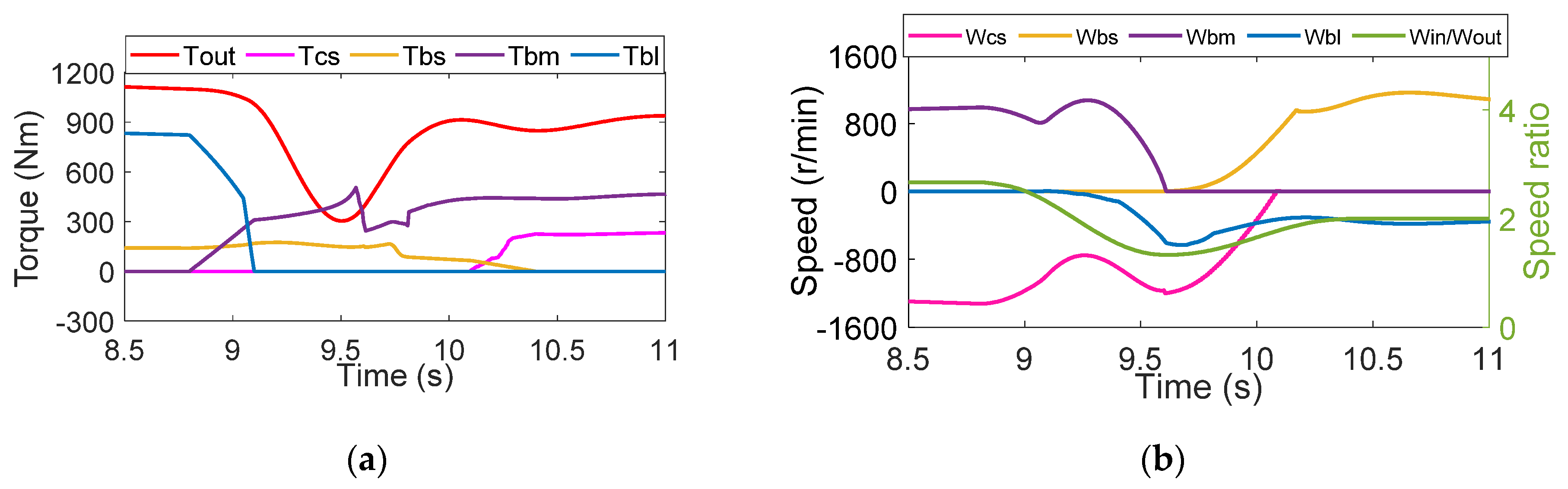
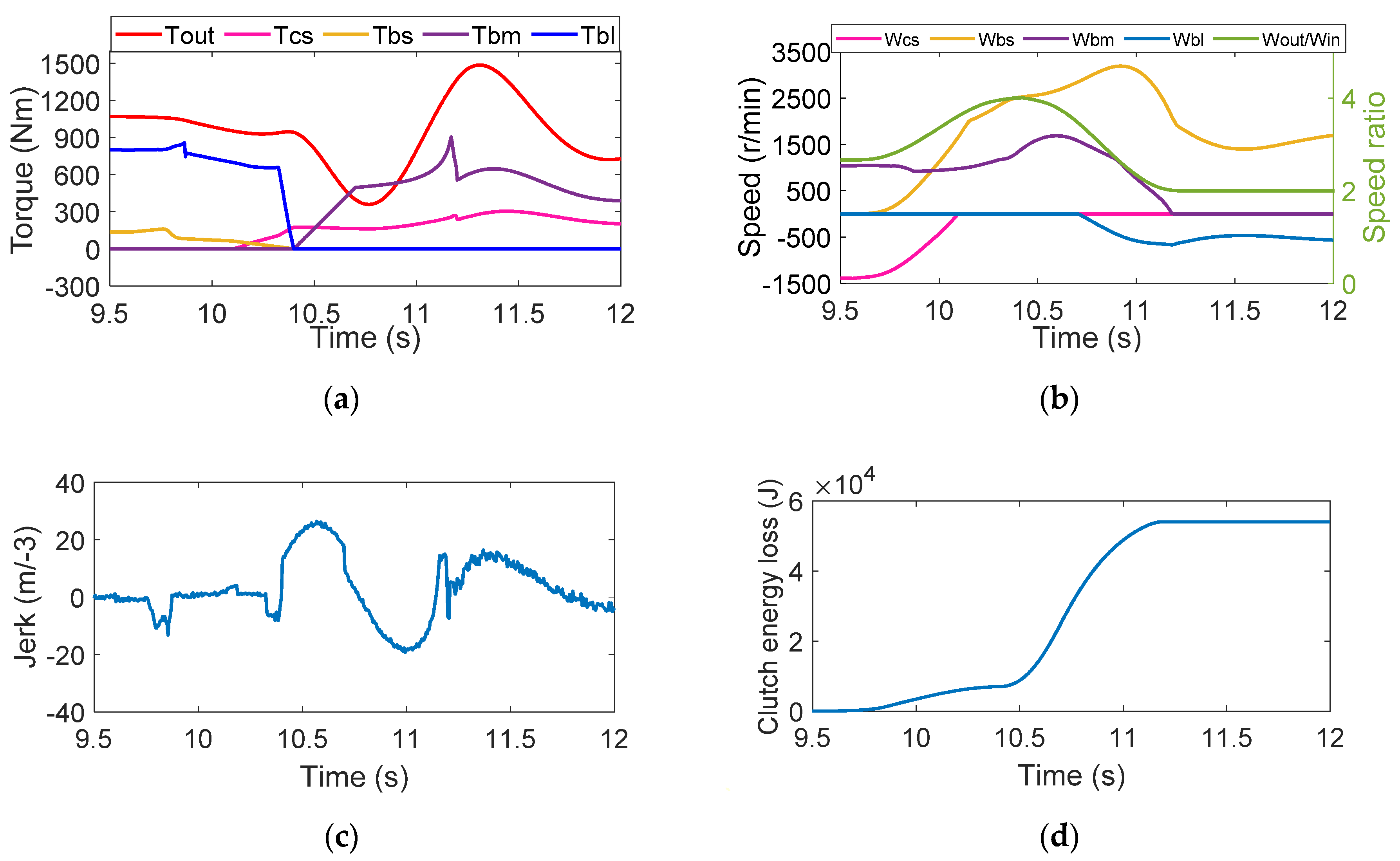
Strategy 1 is to convert the $BL$ and $BM$ first, and then the $BS$ and $CS$, which will result in a 2–4–3 gear change that does not match the expected (2–3). The simulation results of Strategy 1 are shown in Figure 5. After the shifting process from $BL$ to $BM$ is completed, as the transmission reaches 4th gear, the friction torque of $BM$ is not enough to support the increasing demand for the output torque. This leads to the torque hole effect $T_{out}=303 Nm$ at 9.55 s (shown in Figure 5a). In order to stabilize the transmission input torque, the input shaft speed inevitably increases, which also aggravates the engine speed flare (Figure 5b at 9.6 s). During this shifting process, the shift jerk produces a wide range of fluctuations $20.8 {\mathrm{m}/\mathrm{s}}^3>j>-34.3 {\mathrm{m}/\mathrm{s}}^3$. Although the transition of $BS$ and $CS$ are relatively smooth, the entire shift time is longer (1.6 s). The clutches have been slipping for a long time. The clutch friction loss is higher than the expected $W=41.2 KJ$ (see Figure 5d).

4.2. Strategy Two

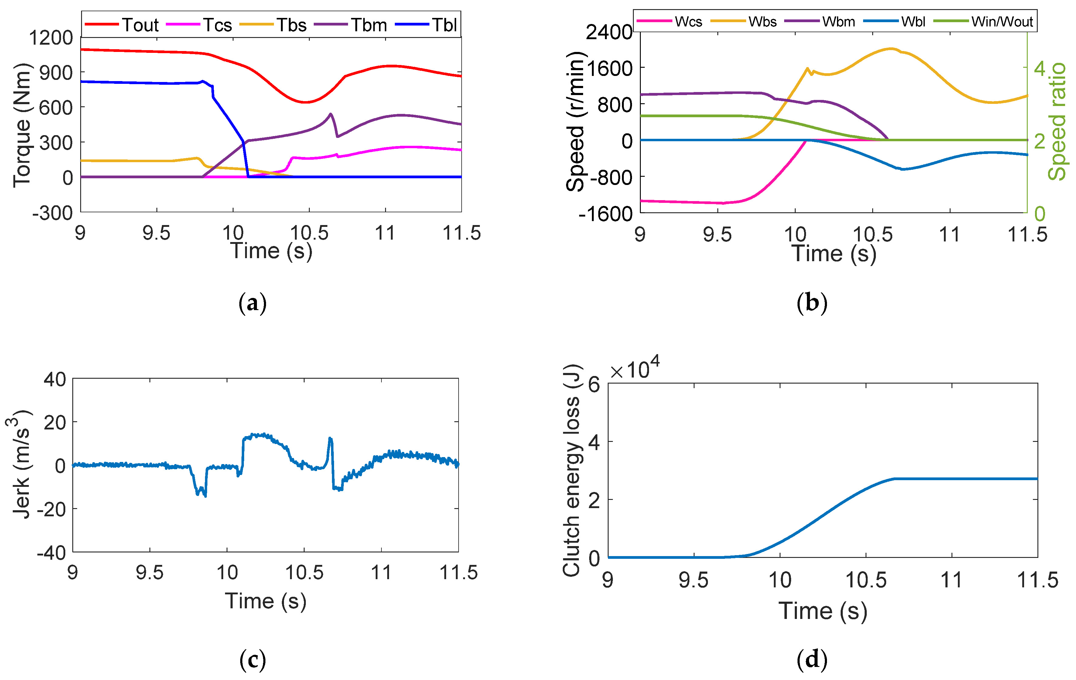
The second strategy is to overlap both the inertia phase of the two sets of clutches after completing the torque phase of the $BL$ and $BM$. The inertia phase is a critical period for the clutch speed changing in Equations (18) and (19). Performing two sets of inertia phases in a shorter period causes the transmission to be more unstable. As shown in Figure 6b, at the beginning of the inertial phase (9.6 s), the $BL$ rotates in the opposite direction of the target speed, and the $CS$ fluctuates around zero speed when it is not locked, which caused torque fluctuations so far as to reverse torque (Figure 6a at 10.05 s). Therefore, there is a large shift jerk in the entire inertial phase. The root mean square of jerk is $\overline{j}>20 {\mathrm{m}/\mathrm{s}}^3$, and its peak value is $j_{\max }=32.5 {\mathrm{m}/\mathrm{s}}^3$ at 10.01 s (Figure 6c). In the two torque phases, since each clutch only needs to complete its own torque switching task, the torque fluctuation is not violent. The shift time is controlled at about 1.2 s, and the clutch slip power is $W=35.0 \mathrm{K}\mathrm{J}$.

4.3. Strategy Three

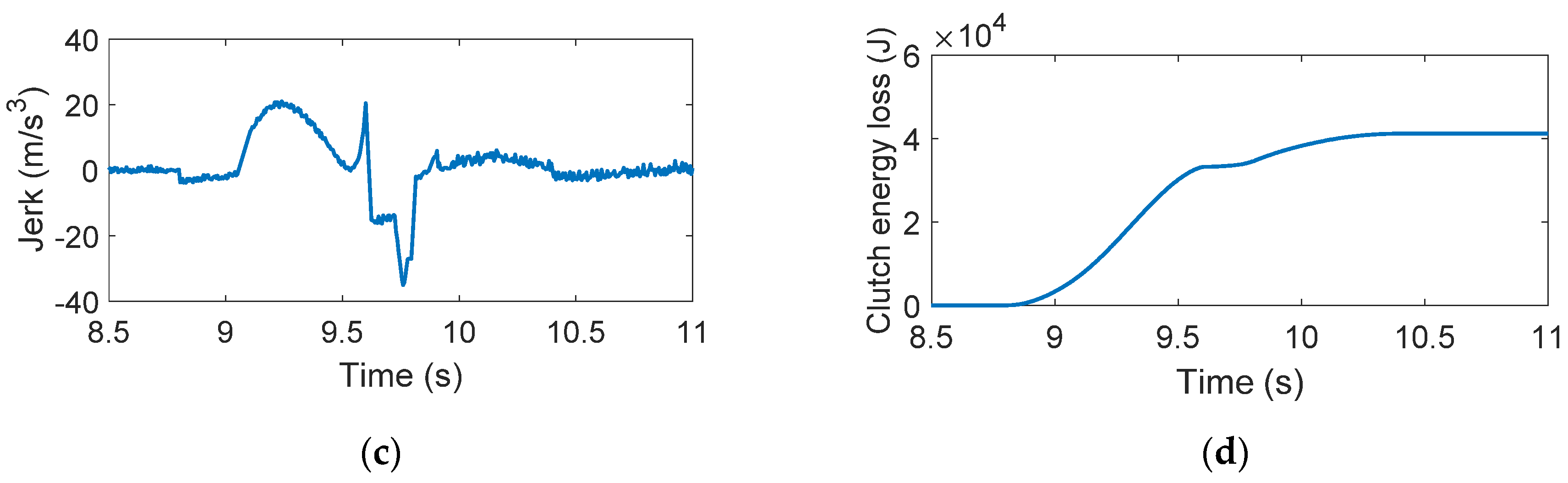
The third strategy is to overlap the torque phase of the $BL$ and $BM$ with the inertia of the $BS$ and $CS$, and then complete the inertial phase of the $BL$ and $BM$ and the torque phase of the $BS$ and $CS$. Compared with other strategies, this strategy has the minimum shift time (approximately 1.0 s), so that the clutch energy loss is only $W=27.1 KJ$. The two inertial phases are completed with the torque phase, the clutch is in a relatively flexible state with multiple degrees of freedom, and the relative speed control of the clutch is more stable (see Figure 7b). The torque interruption or conflict generated by the inertial phase can also be absorbed or compensated by the torque changes of another group of clutches in the torque phase. Thus, there are small torque fluctuations only when the clutch is close to zero speed, as shown in Figure 7a at 9.75 s and 10.65 s. The torque hole $T_{out}=638 Nm$ and the torque bump $T_{out}=930 Nm$ of the output shaft are well controlled. The shift jerk is relatively stable, and it mainly occurs when the torque phase and the inertia phase alternate, and the peak value is not large ($j_{\max }=14.2 {\mathrm{m}/\mathrm{s}}^{-3}$).

4.4. Strategy Four

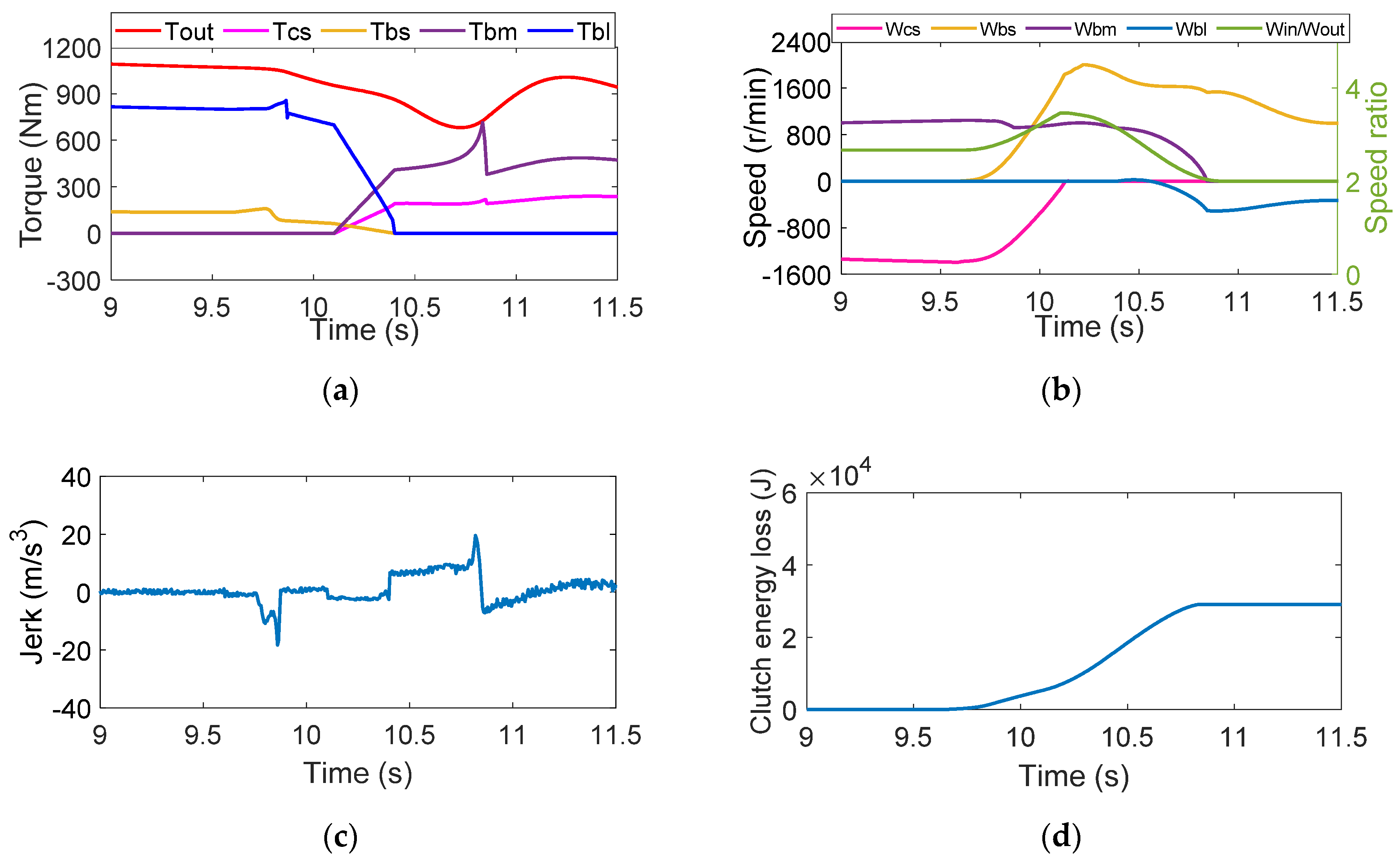
The fourth strategy completes the inertial phase of the $BS$ and $CS$ first; then, it overlaps the torque phase, and finally finishes the inertial phase of the $BL$ and $BM$. Since the shift time of this strategy is about 1.3 s, and the output shaft torque $\Delta T_{out}=325 Nm$ is stable, the shift jerk $j_{\max }=19.4 {\mathrm{m}/\mathrm{s}}^3$ and clutch energy loss $W=31.3 KJ$ can be controlled at a good level (as shown in Figure 8c,d). However, completing the inertial phase of the $BS$ and $CS$ first leads to a 2–1 downshift of the gear; then, the input shaft speed increases rapidly, and the engine flare is obvious from Equation (22). The speed ratio of the transmission is over the 2-3 gears (Figure 8b ${\omega }_{in}/{\omega }_{out}=3.2$, at 10.1 s). Therefore, after completing the shift, the vehicle speed is lower than that in other strategies.

4.5. Strategy Five

Strategy 5 is the opposite of Strategy 1. The transition of the $BS$ and $CS$ go first and then the $BL$ and $BM$. This will result in a 2–1–3 gear change that does not match the expected (2–3), similar to Strategy 4. Since entering the gear is unreasonable, the rapid increase in the input shaft speed causes serious engine flare, and the speed of transmission components changes drastically (see Figure 9b). During the period of 10.5 to 11.5 s, the large change of the output shaft torque causes the shift jerk to deteriorate $26.4 {\mathrm{m}/\mathrm{s}}^3>j>-19.3 {\mathrm{m}/\mathrm{s}}^3$. The longer shift time (1.9 s) also makes the highest clutch energy loss among the five strategies ($W=54.9 KJ$), as shown in Figure 9d.

From Strategy 1 to 5, we can see that the non-overlapping of the two sets of clutch inertia phases in the double-transition shift can effectively reduce the shift jerk (Strategy 3 and Strategy 4). The overlapping of the torque phase and the inertia phase of the other clutch set can control the clutch energy loss at a low level due to using less shift time (Strategy 3).

5. Conclusions

(1)

In this paper, the Lagrange method is used to dynamically model the double-transition shift for heavy-duty mining truck automatic transmission. The vehicle powertrain system and the controller based on the multi-objective genetic algorithm are built-in Matlab/Simulink. The dynamic analysis of two sets of clutches for DTS is carried out.

(2)

Obtained in the multi-objective genetic algorithm, the Pareto optimal solution shows that the lowest root mean square of shift jerk and the energy loss of clutches are $4.05 {\mathrm{m}/\mathrm{s}}^{-3}$ and $22.4 KJ$, respectively.

(3)

The simulation results of five strategies of double-transition shift show that overlapping the inertia phases of both clutch groups will cause the fluctuation amplitude of the output torque to increase. On the contrary, the shift jerk can be more stable at $j_{\max }\le 14.2 {\mathrm{m}/\mathrm{s}}^{-3}$, which is reduced by 56.3%, when the inertial phases are not overlapped. The torque phase overlaps with the inertia phase of another group of clutches, effectively reducing the shift time to about 1.1s and thus decreasing the clutch energy loss by 13.4%, which is $W=27.1 KJ$.

References

- Zhao, X.; Zhang, W.; Feng, Y.; Yang, Y. Optimizing Gear Shifting Strategy for Off-Road Vehicle with Dynamic Programming. Math. Probl. Eng. 2014, 2014, 1–9. [Google Scholar] [CrossRef] [Green Version]
- Meng, F.; Shi, P.; Karimi, H.R.; Zhang, H. Optimal design of an electro-hydraulic valve for heavy-duty vehicle clutch actuator with certain constraints. Mech. Syst. Signal. Process. 2016, 68, 491–503. [Google Scholar] [CrossRef]
- Ouyang, T.; Huang, G.; Li, S.; Chen, J.; Chen, N. Dynamic modelling and optimal design of a clutch actuator for heavy-duty automatic transmission considering flow force. Mech. Mach. Theory 2020, 145, 103716. [Google Scholar] [CrossRef]
- Gao, B.; Liang, Q.; Xiang, Y.; Guo, L.; Chen, H. Gear ratio optimization and shift control of 2-speed I-AMT in electric vehicle. Mech. Syst. Signal. Process. 2015, 615–631. [Google Scholar] [CrossRef]
- Cheng, Y.; Dong, P.; Yang, S.; Xu, X. Virtual Clutch Controller for Clutch-to-Clutch Shifts in Planetary-Type Automatic Transmission. Math. Probl. Eng. 2015, 2015, 1–16. [Google Scholar] [CrossRef] [Green Version]
- Ranogajec, V.; Deur, J.; Ivanović, V.; Tseng, H.E. Multi-objective parameter optimization of control profiles for automatic transmission double-transition shifts. Control. Eng. Pract. 2019, 93, 104183. [Google Scholar] [CrossRef]
- Čorić, M.; Ranogajec, V.; Deur, J.; Ivanovic, V.; Tseng, H.E. Optimization of Shift Control Trajectories for Step Gear Automatic Transmissions. J. Dyn. Syst. Meas. Control. 2017, 139, 061005. [Google Scholar] [CrossRef]
- Mishra, K.D.; Srinivasan, K. Robust control and estimation of clutch-to-clutch shifts. Control. Eng. Pract. 2017, 65, 100–114. [Google Scholar] [CrossRef]
- Oh, J.-Y.; Park, J.-Y.; Cho, J.-W.; Kim, J.-G.; Kim, J.-H.; Lee, G.-H. Influence of a clutch control current profile to improve shift quality for a wheel loader automatic transmission. Int. J. Precis. Eng. Manuf. 2017, 18, 211–219. [Google Scholar] [CrossRef]
- Sanada, K.; Gao, B.; Kado, N.; Takamatsu, H.; Toriya, K. Design of a robust controller for shift control of an automatic transmission. Proc. Inst. Mech. Eng. Part. D J. Automob. Eng. 2012, 226, 1577–1584. [Google Scholar] [CrossRef]
- Tsai, L.-W.; Norton, R. Mechanism Design: Enumeration of Kinematic Structures According to Function. Appl. Mech. Rev. 2001, 54, B85–B86. [Google Scholar] [CrossRef]
- Hsu, C.-H.; Hsu, J.-J. Epicyclic gear trains for automotive automatic transmissions. Proc. Inst. Mech. Eng. Part. D J. Automob. Eng. 2000, 214, 523–532. [Google Scholar] [CrossRef]
- Ranogajec, V.; Deur, J. A Bond Graph-Based Method of Automated Generation of Automatic Transmission Mathematical Model. Sae Int. J. Engines 2017, 10, 1367–1374. [Google Scholar] [CrossRef]
- Ranogajec, V.; Deur, J.; Čorić, M. Bond Graph Analysis of Automatic Transmission Shifts including Potential of Extra Clutch Control. Sae Int. J. Engines 2016, 9, 1929–1945. [Google Scholar] [CrossRef]
- Zhao, X.; Li, Z. Data-Driven Predictive Control Applied to Gear Shifting for Heavy-Duty Vehicles. Energies 2018, 11, 2139. [Google Scholar] [CrossRef] [Green Version]
- Song, X.; Sun, Z. Pressure-Based Clutch Control for Automotive Transmissions Using a Sliding-Mode Controller. IEEE Asme Trans. Mechatron. 2011, 17, 534–546. [Google Scholar] [CrossRef]
- Meng, F.; Tao, G.; Zhang, T.; Hu, Y.; Geng, P. Optimal shifting control strategy in inertia phase of an automatic transmission for automotive applications. Mech. Syst. Signal. Process. 2015, 742–752. [Google Scholar] [CrossRef]
- Wurm, A.; Bestle, D. Robust design optimization for improving automotive shift quality. Optim. Eng. 2015, 17, 421–436. [Google Scholar] [CrossRef]
- Wu, D.; Zhang, Y.; Chang, Y.-P.; Hebbale, K.; Kao, C.-K. Dynamic analysis and simulation of driveability and control of a double transition shifting system. 2009 IEEE Veh. Power Propuls. Conf. 2009, 348–353. [Google Scholar] [CrossRef]
- Wu, D.; Chang, Y.-P. Simulation and Studies on a Double Transition Shift Transmission. Sae Tech. Pap. Ser. 2010. [CrossRef]
- Ranogajec, V.; Ivanović, V.; Deur, J.; Tseng, H.E. Optimization-based assessment of automatic transmission double-transition shift controls. Control. Eng. Pract. 2018, 76, 155–166. [Google Scholar] [CrossRef]
- Patinya, S. Modeling and Control of Automatic Transmission with Planetary Gears for Shift Quality. Ph.D. Thesis, The University of Texas, Austin, TX, USA, 2012. [Google Scholar]
- Kim, J.; Choi, S.B. Design and Modeling of a Clutch Actuator System with Self-Energizing Mechanism. IEEE Asme Trans. Mechatron. 2010, 16, 953–966. [Google Scholar] [CrossRef]
- Hahn, J.-O.; Lee, K.-I. Nonlinear Robust Control of Torque Converter Clutch Slip System for Passenger Vehicles Using Advanced Torque Estimation Algorithms. Veh. Syst. Dyn. 2002, 37, 175–192. [Google Scholar] [CrossRef]
- Liang, J.; Zhang, J.; Zhang, H.; Yin, C. Fuzzy Energy Management Optimization for a Parallel Hybrid Electric Vehicle using Chaotic Non-dominated sorting Genetic Algorithm. Automatika 2015, 56, 149–163. [Google Scholar] [CrossRef] [Green Version]
- Saini, V.; Singh, S.; Nv, S.; Jain, H. Genetic Algorithm Based Gear Shift Optimization for Electric Vehicles. Sae Int. J. Altern. Powertrains 2016, 5, 348–356. [Google Scholar] [CrossRef]
- Deb, K.; Pratap, A.; Agarwal, S.; Meyarivan, T. A fast and elitist multiobjective genetic algorithm: NSGA-II. IEEE Trans. Evol. Comput. 2002, 6, 182–197. [Google Scholar] [CrossRef] [Green Version]
Figure 1.
6 + 2 speed automatic transmission (AT) powertrain system.
Figure 2.
Stribeck friction model (a) and clutch friction working modes switching according to different transmitted torques and relative speeds of clutch (b).
Figure 3.
Multi-objective genetic algorithm diagram (non-dominated sorting genetic algorithm II, NSGA-II).
Figure 4.
Pareto frontiers for five control strategies with a different weighting factor
Figure 5.
Simulation results of 2–3 power-on double-transition upshift for Strategy 1. (a) Output shaft and clutch torque. (b) Clutch speed and speed ratio. (c) The jerk of shift process. (d) The clutch energy loss of shift process.
Figure 6.
Simulation results of 2–3 power-on double-transition upshifts for Strategy 2. (a) Output shaft and clutch torque. (b) Clutch speed and speed ratio. (c) The jerk of shift process. (d) The clutch energy loss of shift process.
Figure 7.
Simulation results of 2–3 power-on double-transition upshift for Strategy 3. (a) Output shaft and clutch torque. (b) Clutch speed and speed ratio. (c) The jerk of shift process. (d) The clutch energy loss of shift process.
Figure 8.
Simulation results of 2–3 power-on double-transition upshift for Strategy 4. (a) Output shaft and clutch torque. (b) Clutch speed and speed ratio. (c) The jerk of shift process. (d) The clutch energy loss of shift process.
Figure 9.
Simulation results of 2–3 power-on double-transition upshift for Strategy 5. (a) Output shaft and clutch torque. (b) Clutch speed and speed ratio. (c) The jerk of shift process. (d) The clutch energy loss of shift process.