An Experimental Approach on Beating in Vibration Due to Rotational Unbalance
by
 , ,
, ,
Dragos-Florin Chitariu
* ,
,
Florin Negoescu
,
Mihaita Horodinca
,
Catalin-Gabriel Dumitras
,
Gures Dogan
and
Mehmet Ilhan
“Gheorghe Asachi” Technical University of Iasi, 700050 Iasi, Romania
*
Author to whom correspondence should be addressed.
Appl. Sci. 2020, 10(19), 6899; https://doi.org/10.3390/app10196899
Submission received: 2 September 2020
/
Revised: 28 September 2020
/
Accepted: 28 September 2020
/
Published: 1 October 2020
(This article belongs to the Special Issue New Materials and Advanced Procedures of Obtaining and Processing)
Abstract
:This paper proposes a study in theoretical and experimental terms focused on the vibration beating phenomenon produced in particular circumstances: the addition of vibrations generated by two rotating unbalanced shafts placed inside a lathe headstock, with a flat friction belt transmission between the shafts. The study was done on a simple computer-assisted experimental setup for absolute vibration velocity signal acquisition, signal processing and simulation. The input signal is generated by a horizontal geophone as the sensor, placed on a headstock. By numerical integration (using an original antiderivative calculus and signal correction method) a vibration velocity signal was converted into a vibration displacement signal. In this way, an absolute velocity vibration sensor was transformed into an absolute displacement vibration sensor. An important accomplishment in the evolution of the resultant vibration frequency (or combination frequency as well) of the beating vibration displacement signal was revealed by numerical simulation, which was fully confirmed by experiments. In opposition to some previously reported research results, it was discovered that the combination frequency is slightly variable (tens of millihertz variation over the full frequency range) and it has a periodic pattern. This pattern has negative or positive peaks (depending on the relationship of amplitudes and frequencies of vibrations involved in the beating) placed systematically in the nodes of the beating phenomena. Some other achievements on issues involved in the beating phenomenon description were also accomplished. A study on a simulated signal proves the high theoretical accuracy of the method used for combination frequency measurement, with less than 3 microhertz full frequency range error. Furthermore, a study on the experimental determination of the dynamic amplification factor of the combination vibration (5.824) due to the resonant behaviour of the headstock and lathe on its foundation was performed, based on computer-aided analysis (curve fitting) of the free damped response. These achievements ensure a better approach on vibration beating phenomenon and dynamic balancing conditions and requirements.
1. Introduction
Rotating unbalance is a topic frequently mentioned in the analysis of the dynamics of rotary bodies (rotordynamics [1]). The rotating unbalance occurs due to an asymmetry of mass distribution (in some different regions of the rotary body, the center of mass is not placed on the axis of rotation). Centrifugal forces occur in these unbalanced regions of the rotary body. The resultant of these centrifugal forces is transmitted through the bearings to the structure where the rotary body is placed. In each bearing the resultant of centrifugal forces has two components at orthogonal directions. Each component acts as a harmonic excitation force against the structure, thus generating vibrations.
For some specific appliances these vibrations are desirable (e. g. in vibration shakers used also as mechanical vibration exciters [2,3], vibration alert systems in mobile phones, electronic vibrating bracelets [4], and haptic feedback devices with vibrations [5]). Generally, the vibrations due to the rotating body unbalances have highly undesirable effects (e.g., bad surface quality in the grinding process [6,7], premature bearing destruction [8,9]), and human body discomfort [10]). In order to measure [11] and to eliminate the unbalance of rotary bodies [12,13,14] (using additional balancing masses and additional inertia [15]), several special requirements must be met and specialized equipment must be used [16,17]. Actually, one of the best ways to balance rotary unbalanced bodies is through the use of self-balancing systems [18,19].
Sometimes two rotary unbalanced bodies having almost the same angular speed (or rotational frequency) which rotate in the same structure (e.g., in centerless grinding machines, [20]) produce a vibration beating phenomenon [10,21,22].
Each rotary unbalanced body generates a vibration. The addition of two vibrations, having slightly different frequencies, produces the aforementioned beating phenomenon. This is a resultant vibration with periodical variation of amplitude, with nodes (where the amplitude has a minimum value, the addition of the two vibrations produces destructive interference, 180 degrees out of phase between the constituents of the resultant vibration) and anti-nodes (a maximum amplitude, where the addition of the two vibrations produces constructive interference, with zero degrees shift of phase between constituents) [23]. Obviously the beating phenomenon in mechanics is not solely related to the vibrations produced by rotary unbalanced bodies, it also occurs when two vibration modes with almost the same modal frequency are excited [24,25], and it occurs as well when a system vibrates simultaneously due to forced sinusoidal excitation close to a resonant frequency and due to a free response [26,27,28,29].
Some specific appliances use the vibration beating phenomenon to monitor the condition of mechanical systems, e.g., monitoring the adhesion integrity of single lap joints [30], monitoring the structural integrity of helicopter rotor blades [31], and for seismic vibration testing [32]. A vibration beating mechanism in piezoelectric energy harvesting systems is proposed in [33].
In machine tools, in addition to a critical source of vibrations (self-excited vibrations in turning [34], milling [35] or grinding [36] processes), the vibrations produced by rotary unbalance (generated by tools [37], shafts [38] or work pieces [36]) and particularly the beating phenomenon [6] created by rotary unbalanced bodies, are important items. This paper proposes some approaches, in theoretical and experimental terms, to address the vibration beating phenomenon produced inside a Romanian lathe headstock SNA 360, by two inner unbalanced rotary shafts, rotating with very close angular speeds. The main achievements of this paper are producing results in the areas of: vibration beating monitoring, conversion of a velocity vibration signal into a displacement signal (by antiderivative calculus), and the evolution of beating vibration signal frequency (pattern, simulation, measurement and accuracy measurement), as well as producing a study of the influence of headstock and lathe foundation dynamics on vibration amplitudes.
2. A Theoretical Approach
Assume that the rotary unbalance of each shaft (each of which rotates at angular speeds of ω1 and ω2, respectively) is reducible at the asymmetry of mass distribution with unbalance masses m1 and m2, respectively, placed in a single plane at distances r1 and r2, respectively, to the rotation axis. The horizontal projection of the centrifugal forces of each rotary unbalance ( and ) generates vibration displacements y1 = kDaf1F1cos(θ1) and y2 = kDaf2F2cos(θ2), where k is the stiffness of the headstock and the lathe foundation, Daf1 and Daf2 are the dynamic amplification factors and θ1 = ω1t+φ1 and θ2 = ω2t+φ2 are the instantaneous values of the angle of the centrifugal forces with respect to the horizontal direction (φ1 and φ2 being the instantaneous values of these angles at t = 0). With these considerations, a complete description of y1 and y2 of the vibrations is given below:
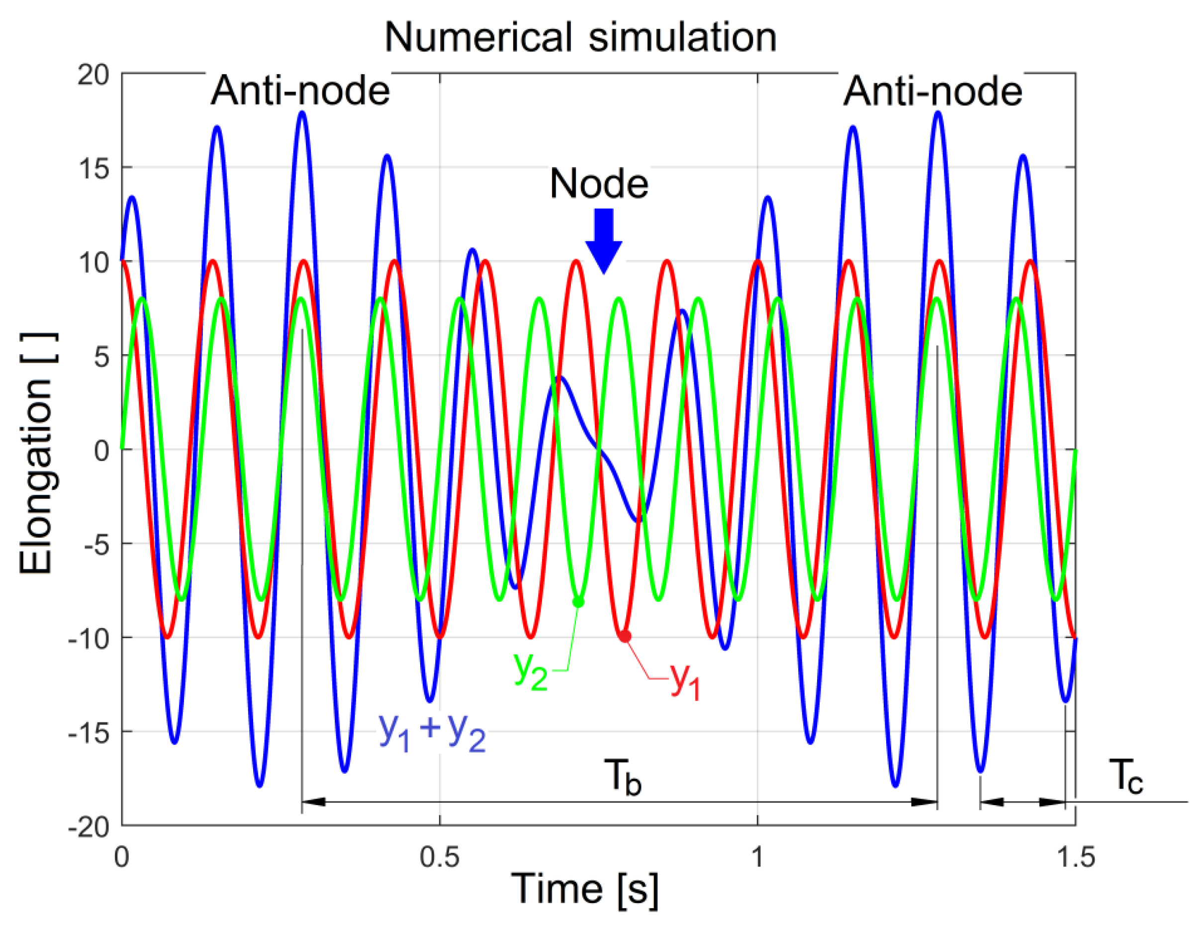
Here and are the vibration amplitudes of the two shafts, respectively. The headstock and the lathe vibrate as a single body on its foundation (as a mass–spring–damper system) with a vibratory motion which is the result of the addition y1 + y2 of these two vibrations, a periodical non-harmonic motion that presents itself as a beating phenomenon [23], with nodes and anti-nodes (as the simulation from Figure 1 proves). According to Figure 1, if the period of vibration y1 is T1 = 2π/ω1 and T2 = 2π/ω2 is the period of vibration y2, then the period Tb of the beating phenomenon (the beat period being the time between two anti-nodes or between two nodes, as well) and the periods T1, T2 (with T2 < T1) should fulfill this obvious condition:
with n being a natural number, defined from Equation (3) as:
In Figure 1 n = 7. If in Equations (3) and (4) the periods are replaced by frequencies (Tb = 1/fb, T1 = 1/f1, T2 = 1/f2), then the resulting frequency fb of the beating phenomenon (beat frequency or the number of nodes per second, as well) is:
In Figure 1 f2 = 8 Hz and f1 = 7 Hz; these generate fb = 1 Hz with Tb = 1s (A1 = 10, A2 = 8, φ1 = 0, φ2 = -π/2).
According to [39], the resultant waveform of the vibration addition y1 + y2 has the frequency fc = 1/Tc (as a combination frequency or modulation frequency, with the period Tc highlighted on Figure 1) defined as:
This paper will prove by simulations and experiments that this definition is not accurate, especially when A1 ≠ A2.
These theoretical considerations and some other supplementary issues and procedures will be confirmed by experimental approach in this paper.
3. Experimental Setup
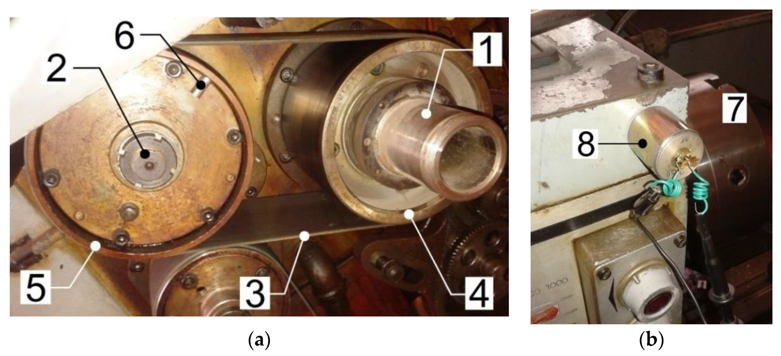
Figure 2a presents a lateral view of both shafts (1 and 2, placed in the headstock) involved in the beating phenomenon due to rotary unbalance.
A friction belt transmission with a flat drive belt 3, a pulley 4 (on shaft 1) and a pulley 5 (on shaft 2) synchronously rotates both shafts (the theoretical value of transmission speed ratio is 1:1). Here 6 depicts an additional mass (10.8 g, a permanent magnet) placed in different angular positions on pulley 5 and used to change the internal unbalancing of the shaft 2.
The shaft 1 is also the lathe main spindle (with the jaw chuck labelled with 7 on Figure 2b placed on the opposite side of Figure 2a). Figure 2b shows an absolute velocity vibration sensor 8 (an electrodynamic seismic geophone Geo Space GS 11D, now HGS Products HG4 as described in [40]), placed on the headstock. The geophone corner frequency (8 Hz) is smaller than the minimum frequency of the headstock vibration (17 Hz). No significant resonant amplification at the corner frequency can be identified (the open circuit damping being 34% of critical damping). The geophone sensitivity is 31.89 V/m/s.
The signal delivered by the vibration sensor (a voltage proportional to the vibration velocity of the headstock) is numerically acquired by a personal computer via a computer-assisted numerical oscilloscope PicoScope 4424 from Pico Technology, Saint Neots, UK (USB powered, four channels, 12 bits resolution, 80 MS/s maximum sampling, 32 MS memory) [41]. Due to the high sensitivity of the geophone and oscilloscope features (e.g., a numerically controlled internal amplifier) the supplementary amplification of the signal delivered by vibration sensor is not necessary.
The computer-aided processing of this signal was done in Matlab. Firstly, the signal delivered by sensor must be mathematically divided by the sensitivity of the sensor in order to obtain the vibration velocity evolution. Secondly, the velocity of vibration must be numerically integrated (by antiderivative calculus) in order to obtain the vibration displacement evolution. The description and analysis of the evolution of some of the other vibration features (e.g., the combination frequency fc, the beat vibration amplitude and the free vibrations of the lathe on foundation) were also performed.
In order to measure the average value of the instantaneous angular speed (IAS) ω1 of the main spindle (shaft 1) rigorously, the technique described in our previous work [42] was used (with a two phase multi-pole AC generator placed in the jaw chuck, as an IAS sensor). The same technique (which refers only to signal processing, briefly described later on) was used for an accurate measurement of the combination frequency fc.
4. Experimental Results and Discussion
4.1. A Beating Phenomenon Described in Vibration Velocity
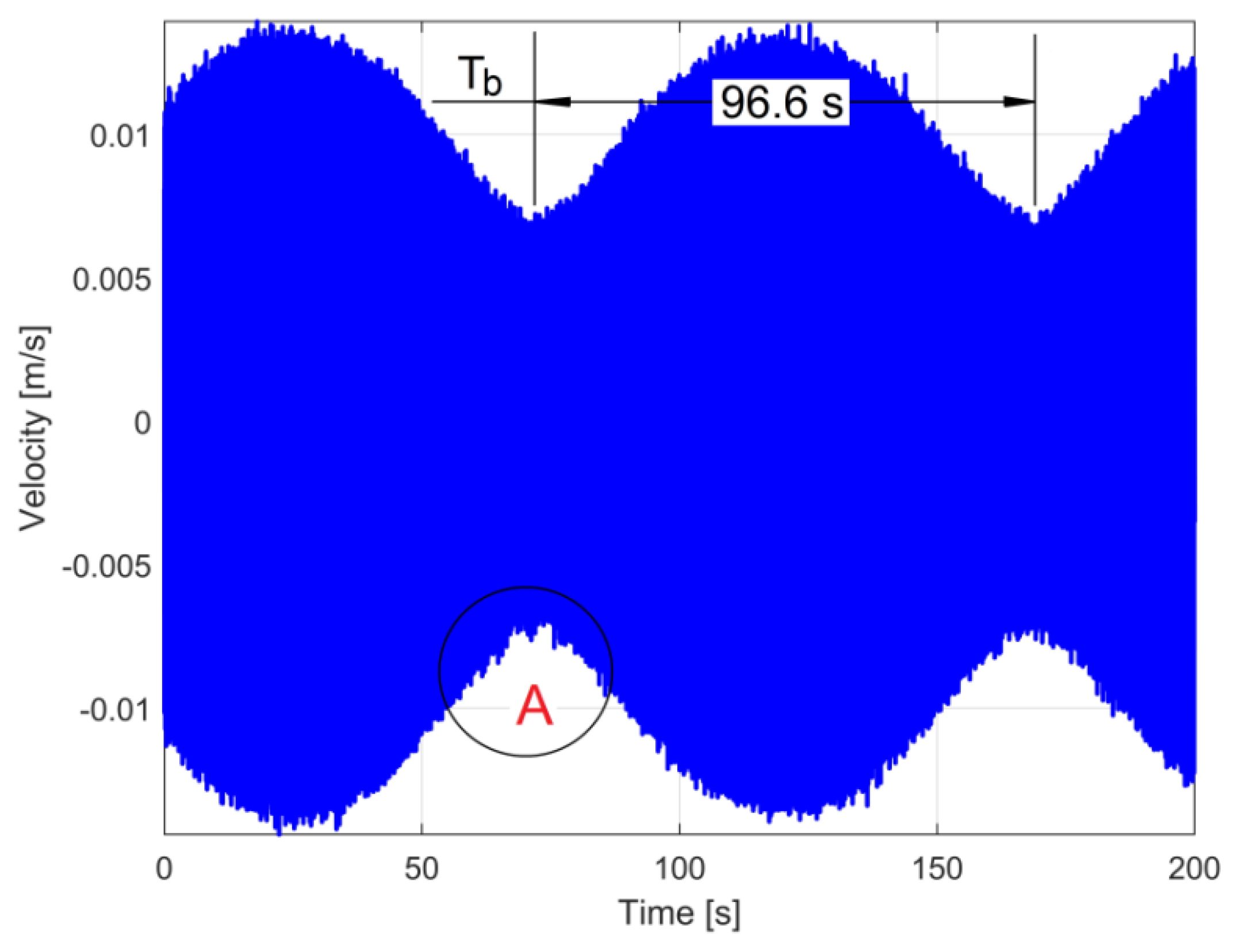
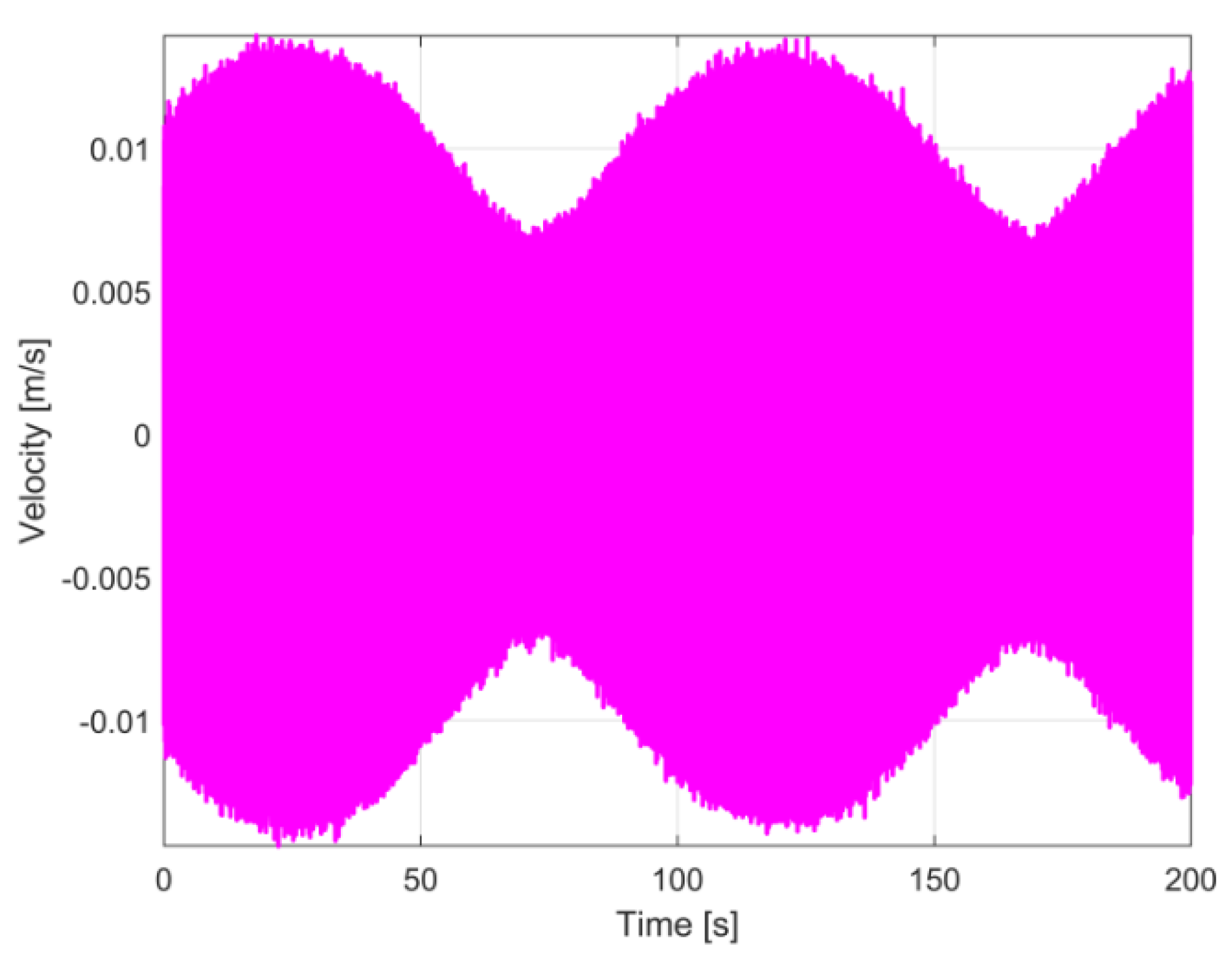
Figure 3 presents the evolution of the headstock vibration velocity during a time interval of 200 s, described with 1 MS (or 1,000,000 samples as well) so a sampling interval of Δt = 200 μs, when the main spindle (shaft 1) rotates (and shaft 2, as well) in the steady-state regime, with constant IAS, with an average value of ω1 = 109.2369 rad/s (for f1 = 17.3856 Hz average rotation frequency, or 1043.1 revolutions per minute on average).
It is obvious that Figure 3 depicts a vibration beating phenomenon with nodes and anti-nodes, with a very high value of the period Tb (96.6 s) and consequently with a very small value of beat frequency fb = 1/Tb = 1/96.6 Hz. The beating phenomenon proves that the IASs ω1 and ω2 and also rotation frequencies f1 and f2 as well, are slightly different because the diameters of pulleys 4 and 5 involved in belt transmission are not strictly the same. With T1 = 1/f1 and the relationship between T1 and Tb from Equation (3) there are n ≈ Tb·f1 ≈ 1679 periods T1 between nodes (and between anti-nodes as well). This is an approximated value of n because the frequency f1 is not rigorously constant (as is proved, later in this paper). According to Equation (3), at each n complete rotations of shaft 1, the shaft 2 makes n + 1 or n − 1 rotations (one rotation difference), which means that the experimentally revealed value of the belt transmission speed ratio is ω2/ω1 = T1/T2 = n/(n ± 1) ≈ 1679/(1679 ± 1). This is also the ratio between pulleys diameters: the diameter of pulley 4 divided by the diameter of pulley 5 (assuming that there is no slipping between the belt and the pulleys).
The additional mass 6 (Figure 2a) was placed in a certain angular position on pulley 5, in order to obtain a maximum value of the amplitude A2, and a maximum difference between amplitudes in anti-nodes and nodes as well. It is obvious that the main spindle (shaft 1) is also unbalanced; otherwise the beating phenomenon does not occur.
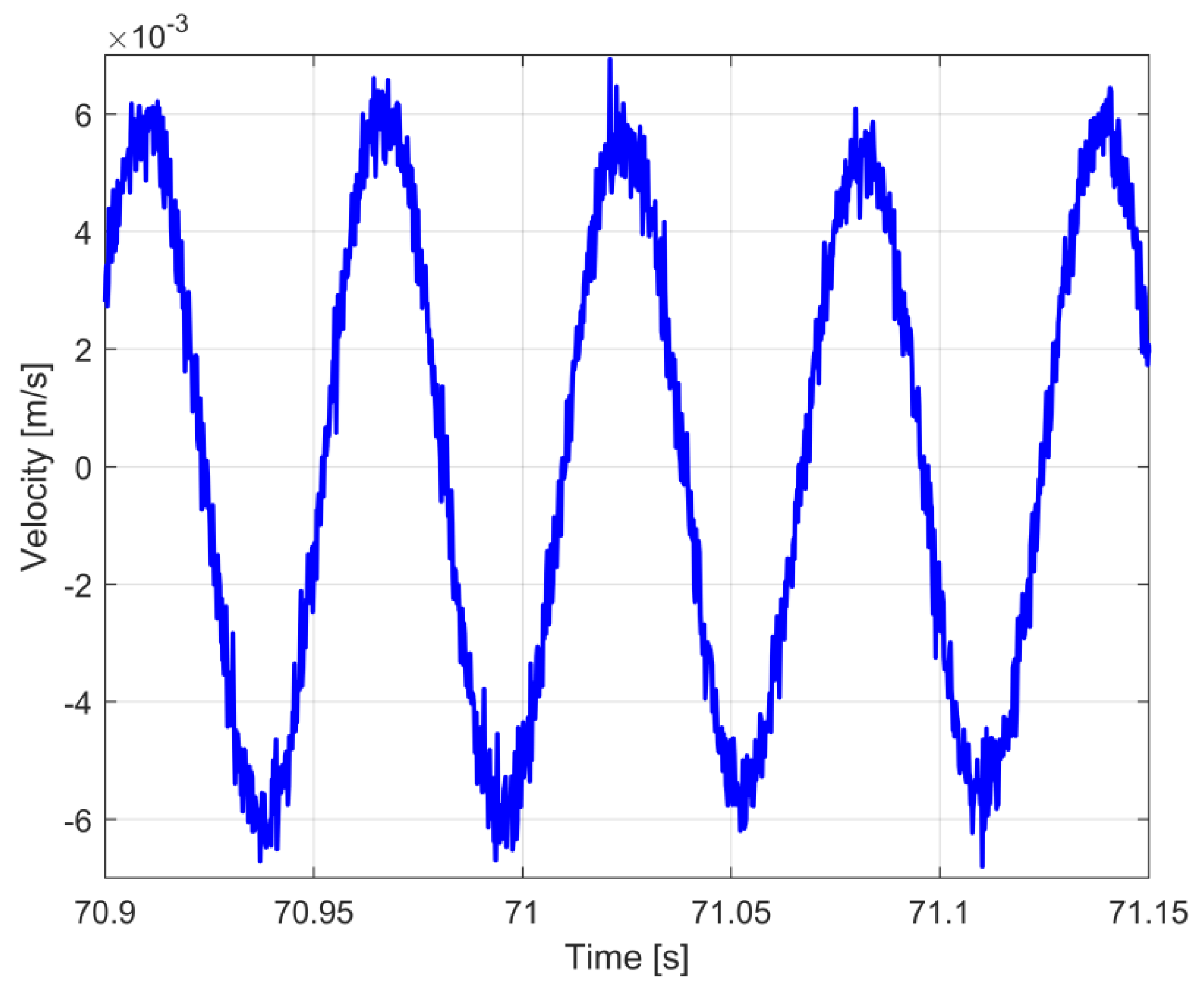
Figure 4 presents a zoomed-in detail in the area labelled A in Figure 3. Here the dominant component (≈6 mm/s amplitude) is the sum of two vibrations created by rotary unbalances; the other low amplitude (and high frequency) components are related by vibrations generated by some other headstock rotary components.
With the values for f1 and fb revealed before, the frequency f2 is a result of Equation (5), with two possible values (f2 = f1 − fb = 17.3752 Hz or f2 = f1 + fb = 17.3959 Hz). Because in Equation (5) the notations f1 and f2 are arbitrary, this equation should be reconsidered as .
As a consequence, the angular speed ω2 = 2πf2 has two possible values (ω2 = 109.1716 rad/s or ω2 = 109.3016 rad/s), as does the speed ratio (ω2/ω1) of the driving belt (with ω1 = 109.2369 rad/s). To find the right value of f2 (and ω2 as well) the technique described in [42] should be used (with an IAS sensor placed on shaft 2).
The evolution from Figure 3 is an addition of vibrations velocities (v = dy1/dt + dy2/dt) generated by both of the unbalanced shafts (1 and 2). It is expected that the beating phenomenon keeps the main characteristics (e.g., Tb, Tc values or fb, fc values, as well) if it is described using the addition of vibration displacements (s = y1 + y2), except for the amplitudes in nodes and anti-nodes which significantly decreases.
4.2. The Description of the Beating Phenomenon in Vibration Displacement by Numerical Integration
The vibration displacement evolution can be obtained from vibration velocity evolution by numerical integration (antiderivative calculus). Based on the approximate definition of velocity (derivative of displacement) v = ds/dt ≈ Δs/Δt, a current sample of velocity vi is defined using two successive samples of displacement si, si−1 (in the displacement interval Δs = si − si−1) and the values of time ti, ti−1 for these samples, in the sampling interval Δt = ti − ti−1 (usually this is a constant value) as:
This is an approximation of the first derivative of displacement as backward finite difference, with i > 1 [43]. The current sample of displacement si can be simply mathematically extracted from Equation (7) as:
Equation (8) describes a sample si of displacement related to velocity, this also being our proposal for a description of numerical integration of velocity (antiderivative calculus). According to Equation (8) the sample si depends on sampling interval Δt (here Δt is the time ti − ti−1 between two consecutive samples of velocity vi and vi−1 or two consecutive samples of displacement si and si−1 as well), the velocity sample vi and the previous sample of displacement si−1, as the result of a previous step of numerical integration. The numerical integration from Equation (8) is available for i > 1. Of course, it is mandatory to know the value of the first sample of displacement s1, this being an indefinite value because i > 1. This is exactly the constant C of integration (usually an arbitrary value). Pure harmonic signals are numerically integrated, in that case, evidently C = 0.
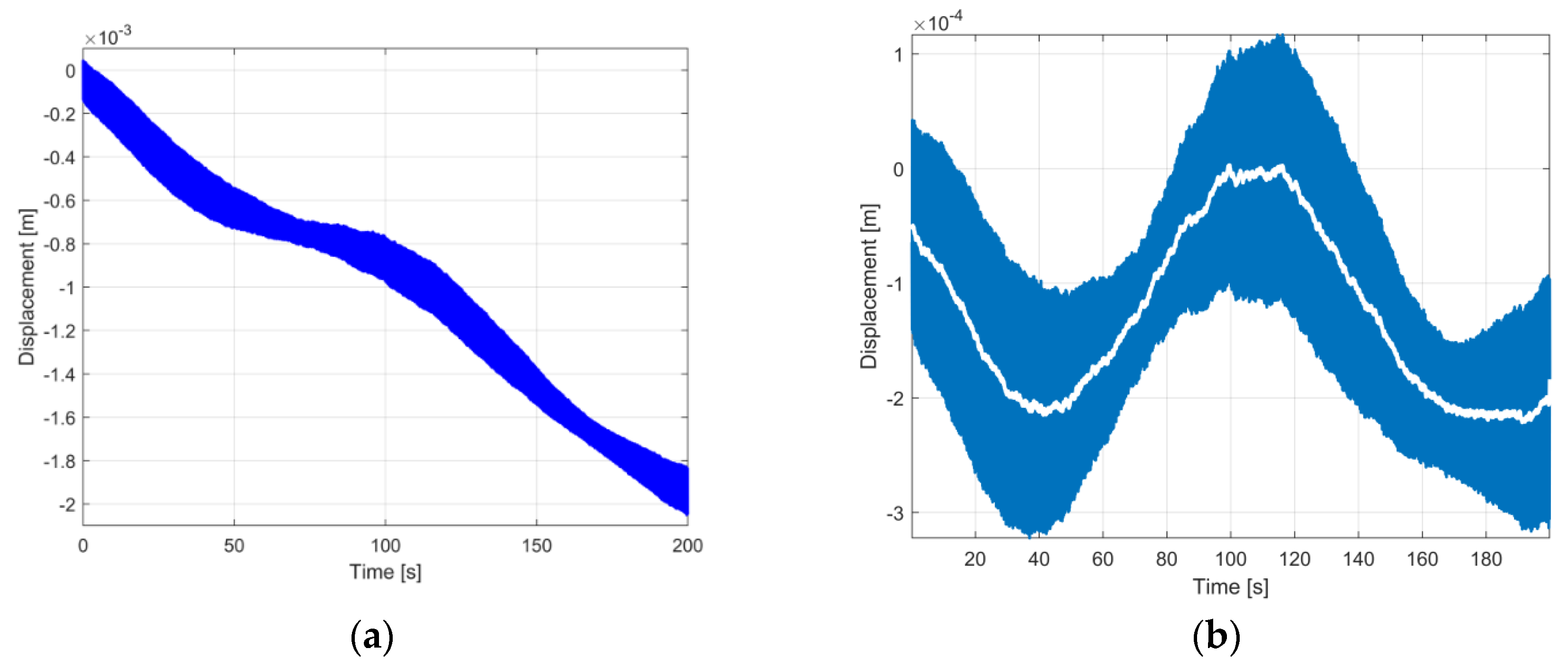
Figure 5a describes the graphical result of numerical integration of vibration elongation evolution from Figure 3 using Equation (8), with . Certainly this evolution is not strictly related to the vibration displacement from the beating phenomenon.
We found that the oscilloscope generates a very small negative constant zero offset. As the theory of integration establishes, the numerical integration of this constant zero offset produces a component with linear evolution, experimentally confirmed in Figure 5a by the evolution with negative slope. The removal of this linear component produces the result from Figure 5b (the evolution emphasized in blue).
It is evident that Figure 5b is not the expected evolution of the vibration displacement in beating phenomenon. Surely, there is not a mistake in the numerical integration proposal in Equation (8) because the numerical derivative of the evolution from Figure 5b using Equation (7) produces exactly the evolution of velocity, as Figure 6 indicates (by comparison with Figure 3).
Our first attempt to explain this deficiency in this result of numerical integration is related by the constant of integration C.
Intuitively it is supposed that somehow the hypothesis that C = 0 is wrong. Perhaps the effect of this wrong hypothesis is mirrored in the evolution from Figure 5b and its effect should be removed (as the influence of negative zero offset was removed before).
It was discovered by numerical simulation that the numerical integration of a computer-generated beating vibration velocity signal (similarly to those depicted in Figure 3) using Equation (8), with C = 0, produces a vertically shifted evolution with a constant nonzero value, which should be mathematically removed.
This approach assumed that in the result of numerical integration of vibration velocity depicted in Figure 5b, a supplementary low frequency component was generated and should be removed. For the time being we unfortunately do not have a consistent explanation for the appearance of this low frequency component. This low frequency component (depicted in Figure 5b in white) was detected by low-pass numerical filtering of the vibration displacement signal (the evolution emphasised in blue).
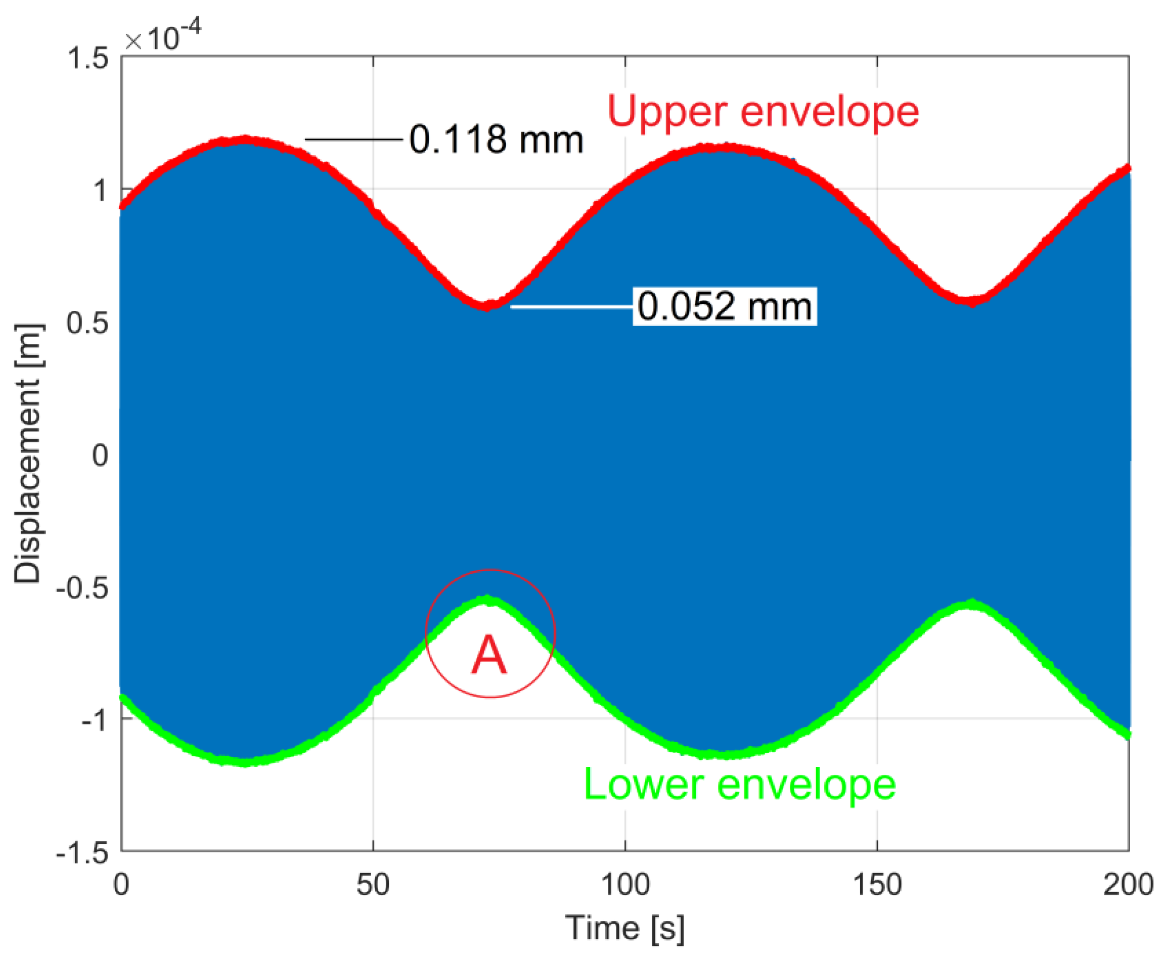
A computer-generated moving average filter [43] was used, with the first notch frequency equal to the combination frequency fc = (f1 + f2)/2 (assuming that this definition from Equation (6) is accurate), in order to completely remove the variable component from Figure 5b having the resultant vibration frequency, and in order to obtain the low frequency component. The number of points in the average of the filter is defined as integer of the ratio 1/(fcΔt). The removal of this low frequency component from the result of numerical integration (the vibration displacement signal) depicted in Figure 5b is shown in Figure 7. It is obvious that this evolution properly describes the resultant vibration displacement during the beating phenomenon, previously described in Figure 3, by the velocity of the resultant vibration.
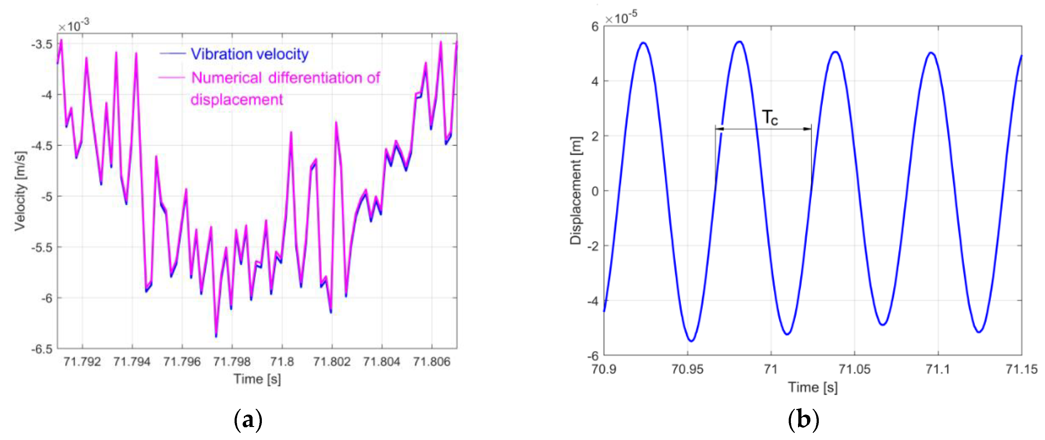
There is a supplementary confirmation of this result: the numerical differentiation of the vibration displacement signal from Figure 7 (using Equation (7)) fits very well with the vibration velocity signal from Figure 3, as a very short detail (15 ms duration) of both evolutions (given in Figure 8a) from the area labelled as A (Figure 3 and Figure 7) indicates. Thus, the absolute velocity vibration sensor together with the proposed numerical signal integration method acts as an absolute displacement vibration sensor.
Figure 8b presents a short detail of the vibration displacement evolution in the area labelled with A in Figure 7. This figure has the same size on the abscissa as Figure 4. By comparison with Figure 4, the evolution is much smoother here, as a consequence of numerical integration, which drastically reduces the amplitudes of high frequency components. The integration acts as a low-pass filter.
In Figure 7 two relationships between the vibrations amplitudes A1 and A2 are available (from Equations (1) and (2)) due to the constructive interference in anti-nodes (A1 + A2 = 118 μm) and destructive interference in nodes (A1 − A2 = 52 μm), so A1 = 85 μm and A2 = 33 μm. For the time being A1 does not necessarily refer to vibration amplitude generated by the main spindle or shaft 1.
4.3. The Evolution of Frequency for Resultant Vibration in Beating Phenomenon
An interesting item in the beating phenomenon is the evolution of frequency of the resultant vibration fc (also known as combination frequency or modulation frequency, fc = 1/Tc, with Tc highlighted in Figure 8b). In [39] this frequency is defined as the average of both frequencies (f1, f2) involved in the beating (Equation (6)).
A beating phenomenon was simulated using the sum of two harmonic vibrations displacements y1s(A1,f1) and y2s(A2,f2)—already described in Equations (1) and (2) with different values of amplitudes (A2 > A1) and frequencies f1 and f2, close to those from the experiment described in Figure 3 and Figure 7 (with f1 = 17.3856 Hz and f2 = 17.3959 Hz), for a duration equal to Tb (placed between two anti-nodes).
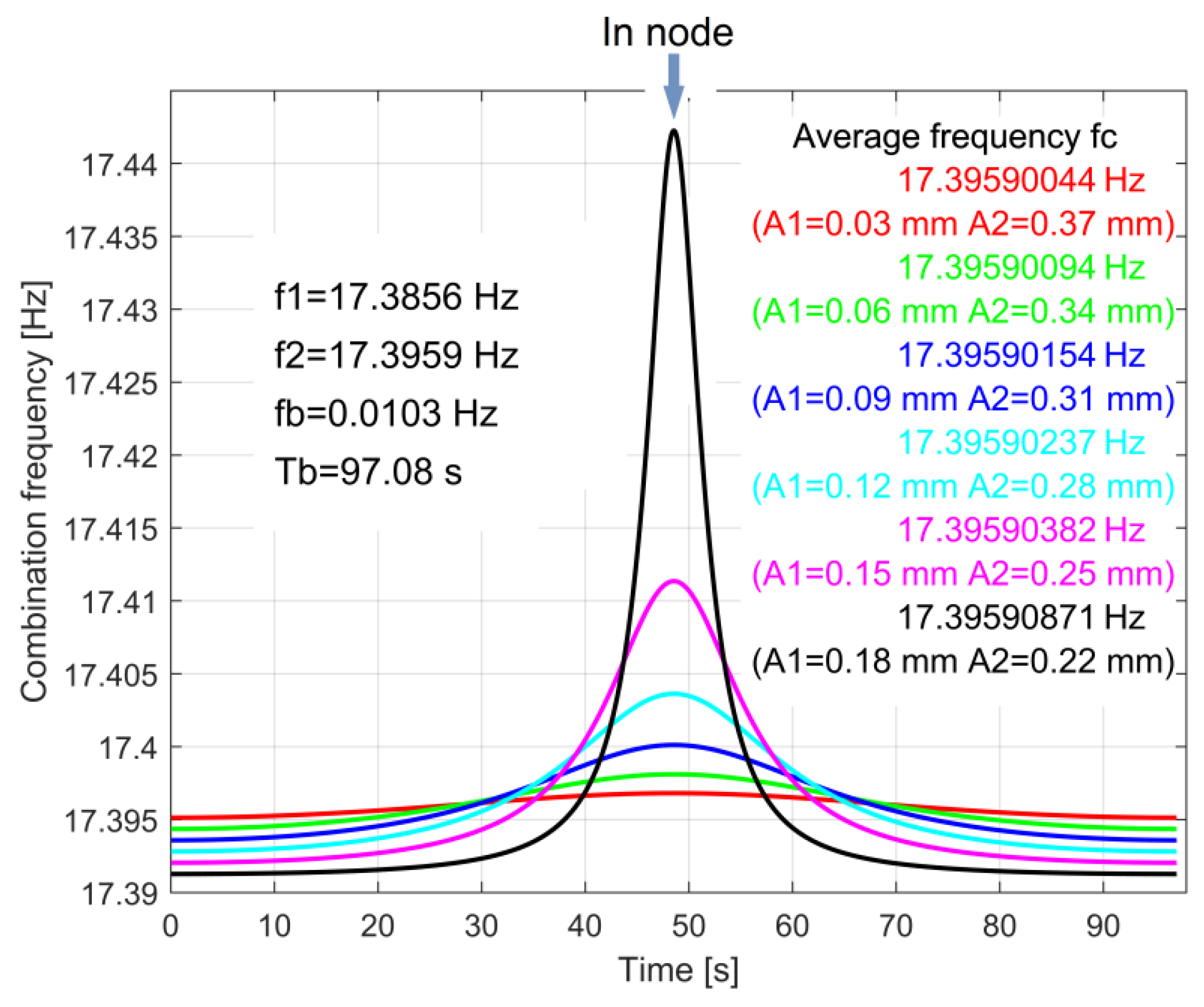
For six different values of amplitudes (A1 increases and A2 decreases), the evolution of the combination frequency fc and its average value was determined on the vibration beating simulated signal, as Figure 9 indicates, using a high accuracy measurement technique from a previous work [42]. Here each peak describes the value of frequency fc in vibration beating node. It is obvious that fc is not constant and, in contradiction with Equation (6) and [39], fc ≠ (f1 + f2)/2. Here, with A1 > A2 the average fc is very close to f2, with fc > f2.
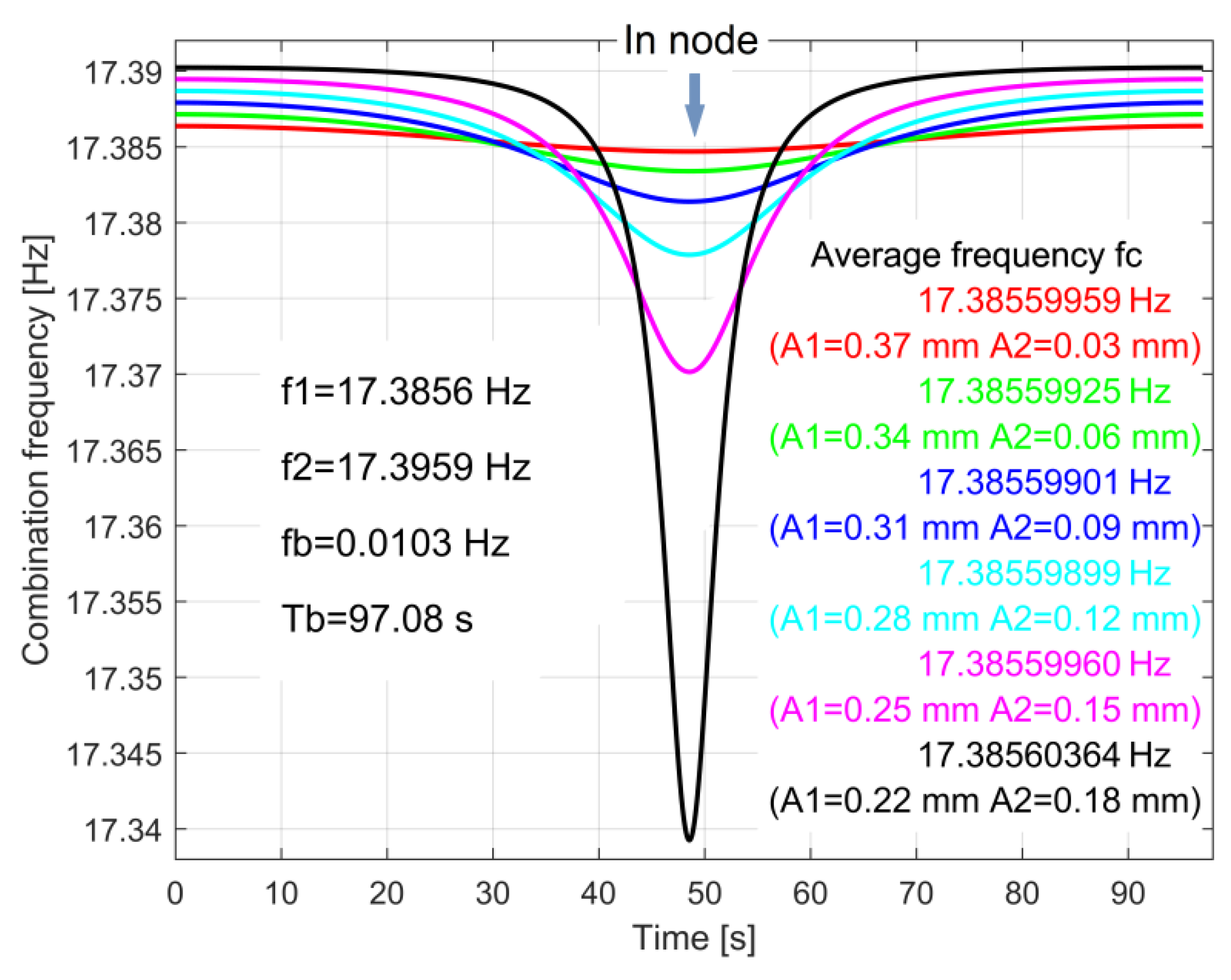
A similar simulation was done in the same conditions, now with A1 > A2, as Figure 10 indicates (here A1 decreases and A2 increases). Similar to the simulation given in Figure 9, it is obvious that fc is not constant and again, in contradiction with Equation (6) and [39], fc ≠ (f1 + f2)/2. The average frequency fc is very close to f1, with fc < f1.
There are two conclusions here, in contradiction with the literature [39]:
- -
- The combination frequency fc is not constant over a period Tb (even if its variation is not significant);
- -
- The average value of the combination frequency fc over a period Tb is practically the same as the frequency of the input vibration in the beating phenomenon (y1s(A1,f1) or y2s(A2,f2)), whose amplitudes are higher (e.g., if A2 > A1 then the average fc ≈ f2).
Some supplementary simulations for many other values of frequencies f1 and f2 (and consequently Tb) completely confirm these conclusions.
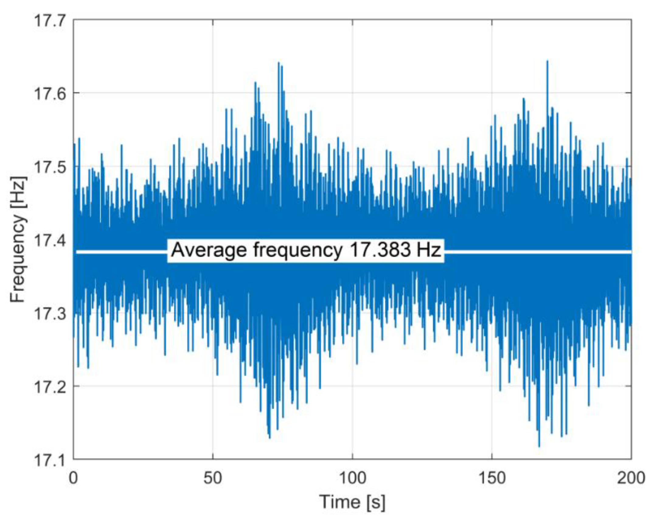
Figure 11 presents the evolution of the instantaneous combination frequency fc during the vibration beating phenomenon (displacement of headstock) experimentally described in Figure 7.
Apparently, this is a very noisy evolution. The dominant component of the signal from Figure 7 is the displacement of resultant vibration y1 + y2. The frequency measurement method [42] is based on detection of zero-crossing moments of this signal (a topic discussed later on). It is obvious that many other additional vibrations of the lathe headstock (some of them with high frequency) disturb the accuracy of the zero-crossing detections, as a main reason for the noisy evolution from Figure 11.
The best information available in Figure 11 is the average value of the combination frequency fc (17.3830 Hz, very close to the rotational frequency of the main spindle, f1 = 17.3856 Hz). Based on the previous conclusions from Figure 9 and Figure 10 it is evident that the amplitude A1 of unbalanced vibration generated by the main spindle (shaft 1) is higher than the amplitude A2 of shaft 2 (so A1 = 85 μm and A2 = 33 μm, an item analysed before). As previously mentioned, the rotational frequency of shaft 2 is f2 = f1 − fb = 17.3752 Hz or f2 = f1 + fb = 17.3959 Hz.
Figure 12 presents a low-pass filtered evolution of the instantaneous combination frequency from Figure 11, (using a multiple moving average filter [43], as a well-known method to attenuate the signal noise).
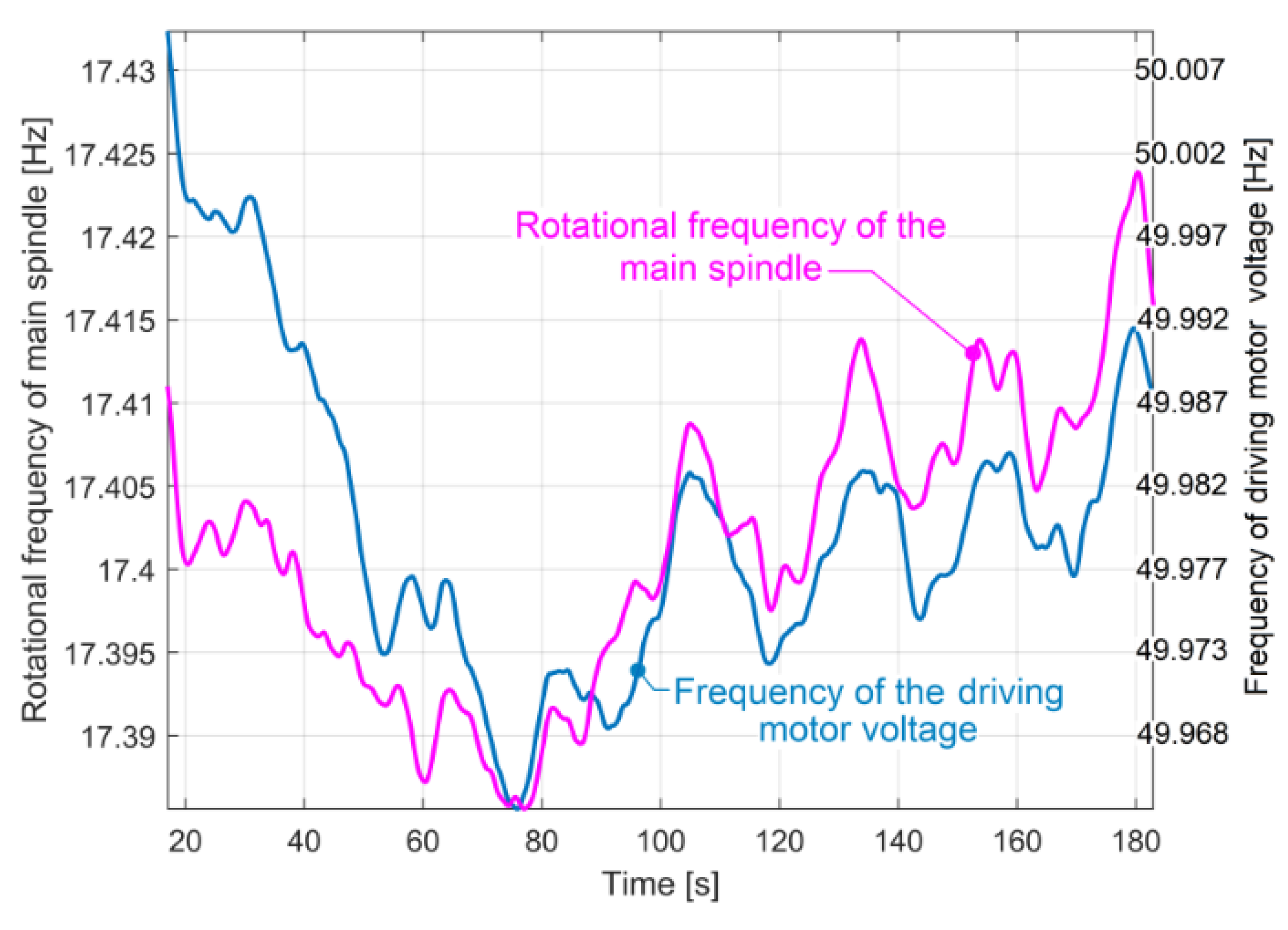
Despite a relatively strong irregular variation of the combination frequency fc (due to the variation of experimental conditions: e.g., the small variation of rotational speeds of shafts 1 and 2, caused mainly by the variation of frequency of the supplying voltages applied to the asynchronous driving motor, around a theoretical value of 50 Hz, as Figure 13 clearly indicates), the previous simulations and conclusions are fully experimentally confirmed. Three supplementary identical experiments confirm the evolution presented in Figure 12.
Firstly, in Figure 12 there are two negative peaks (for the two nodes in Figure 3 or Figure 7; each node produces a negative peak on fc evolution, an item already discussed in the simulation from Figure 10) at a time interval very close to the beat period value Tb, already defined in Figure 3 (96.73 s here, compared with 96.6 s in Figure 3).
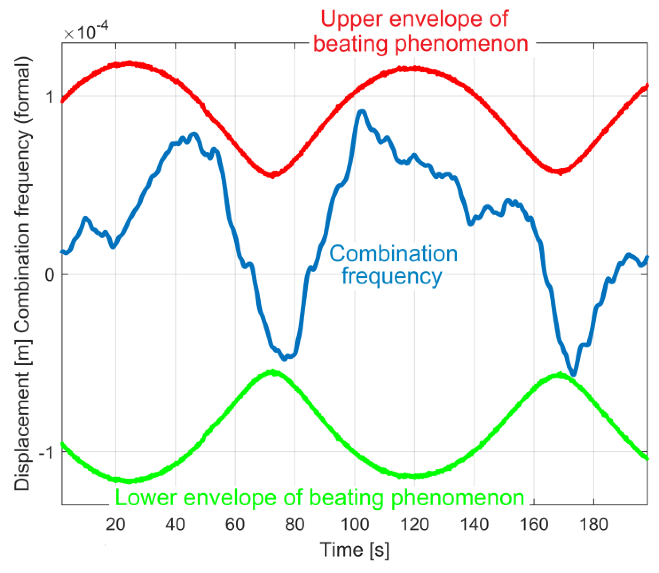
Secondly, as shown in Figure 14, a superposition of filtered frequency fc evolution from Figure 12 (here in a conventional blue coloured description) over the experimental envelopes of vibration displacement in beating (the same as those depicted in Figure 7) indicates that the negative peaks of fc are placed, as expected, in nodes.
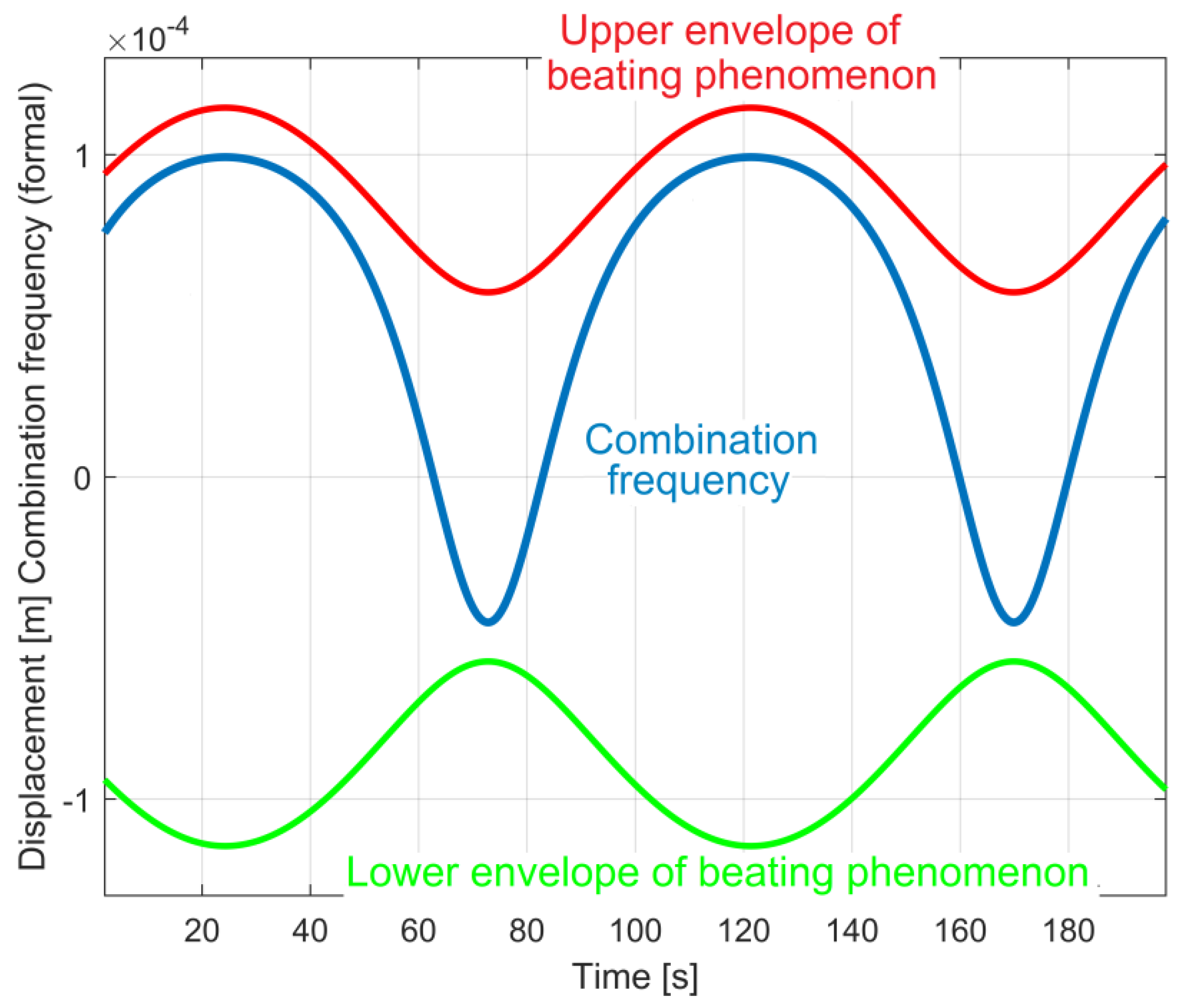
The small displacement to the right of the negative peaks of the filtered combination frequency evolution (as against the nodes on Figure 14) is not related to the numerical filtering. This is proved by the result of the simulation of Figure 14, as given in Figure 15 (with addition of pure harmonic signals y1s and y2s in vibration beating simulation).
This periodic pattern of filtered combination frequency fc evolution experimentally revealed in Figure 12 and Figure 14 (according to the simulations from Figure 10 and Figure 15) is strongly attenuated if the amplitude A2 becomes significantly lower than A1 (and vice versa).
An important question is in order here due to a very small variation of filtered frequencies revealed before (less than 50 mHz full scale evolution in Figure 9, Figure 10, Figure 12, Figure 13 and Figure 15): how accurate is this frequency measurement method [42]?
In this measurement method (e.g., the measurement of the combination frequency fc of vibration displacement signal from Figure 7), the computer-aided detection of the time interval between each two consecutive zero-crossing moments (tzcj and tzcj+1) of a periodical signal is used. This time interval defines a semi-period Tc/2 = tzcj+1 − tzcj as Tc/2 = 1/2fc, or a value fc = 1/Tc. When the result of multiplication of two successive displacements samples si and si−1 (having the sampling times ti and ti−1, with i > 1) is negative or zero (si·si−1 < 0 or si·si−1 = 0) a zero-crossing moment is detected (e.g., tzcj) and calculable as the abscissa of the intersection of a line segment defined by the points of coordinates (ti, si) and (ti−1,si−1) on the t-axis (as x-axis in Figure 8b). The main reason for frequency measurement error εf ≠ 0 is a consequence of calculation errors for two successive zero-crossing moments εj ≠ 0 (for tzcj) and εj+1 ≠ 0 (for tzcj+1). These εj and εj+1 errors are caused by the replacement of a harmonic evolution with a linear evolution between those two successive displacement samples involved in each zero-crossing moment definition. With ti−1−ti = Δt (Δt being the sampling interval) the error εj = 0 only in three situations: (1) if si = 0 (the end of the line segment is placed on the t-axis, with tj = ti), (2) if si−1 = 0 (the start of line segment is placed on t-axis, with tj = ti−1) and (3) if −si = si−1 (the middle of the line segment is placed on t-axis, with tj = ti−1 + Δt/2). A similar approach is available for the next two successive samples (si+h and si+h−1) involved in the definition of tzcj+1 moment and εj+1 error (with h as the integer part of the ratio Tc/Δt). If simultaneously εj and εj+1 = 0 then εf = 0. Any other definition of sampling times generates frequency measurement errors εf ≠ 0.
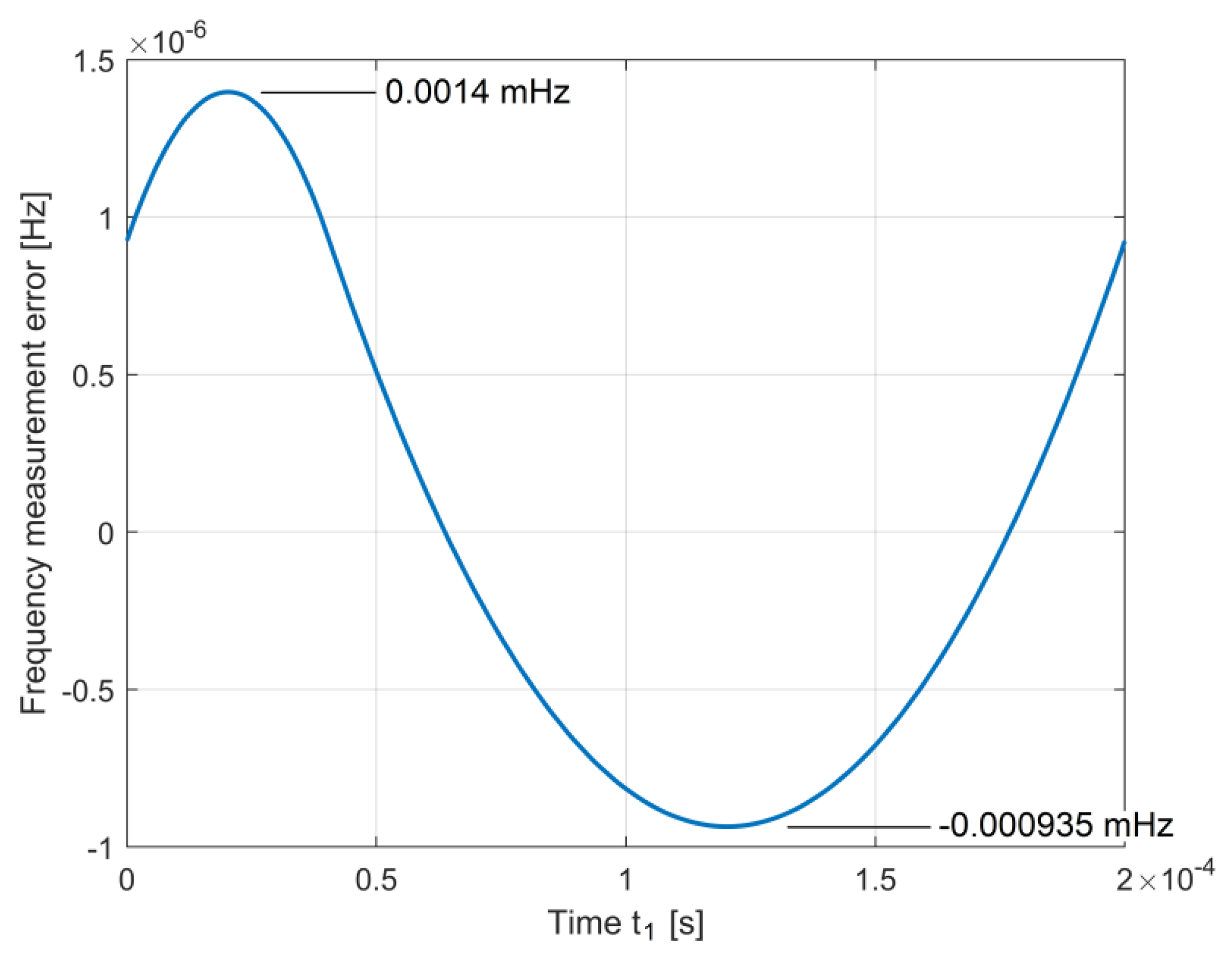
A computer-aided calculus was performed for frequency measurement error εf of a harmonic simulated signal with frequency 17.383 Hz (the average value of the combination frequency fc) during a semi-period. Here 10,000 different values of sampling time t1 (between 0 and Δt, with Δt = 200 μs, the same sampling interval as in Figure 3 and Figure 7) and t2 = Δt − t1 (between Δt and 0) for the first two successive displacement samples involved in the calculus of the first zero-crossing moment tzc1 was used. Figure 16 describes the evolution of the frequency measurement error εf(t1).
As Figure 16 clearly indicates, the frequency measurement error εf of the combination frequency fc is variable and placed between −0.000935 and +0.0014 mHz. The result of the measured frequency of the simulated signal is as a description of the accuracy measurement. Very similar limits for the εf error are calculated for a harmonic signal with frequency f1. If the value of the frequency fc = 1/Tc used in simulation accomplishes the condition Tc = hΔt (with h being an integer), then εf = 0 for any value t1 = 0 ÷ Δt.
4.4. The Influence of the Lathe Suspension Dynamics on Beating Vibrations Amplitude
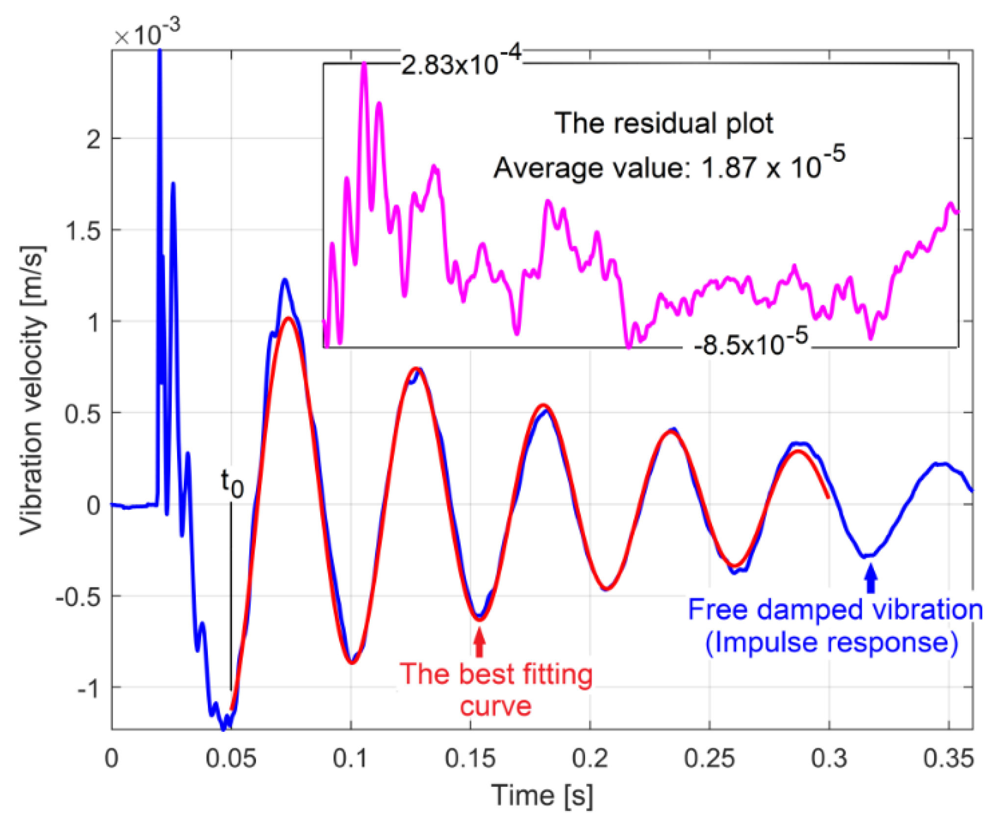
The relative high vibration displacement amplitude of the headstock during the beating phenomenon (as shown in Figure 7) has an evident explanation: the vibration frequencies f1, f2 and fc as well, are close to the first resonant frequency (vibration mode) of the headstock and lathe on its foundation (as a single body mass–spring–damper vibratory system). This means that the dynamic amplification factors Daf1 and Daf2, (involved in Equations (1) and (2)) are significantly higher than 1 (because of resonant amplification). In order to prove that, the resources of a very simple experiment performed with the same experimental setup are available: the evolution of headstock vibration velocity after an impulse excitation produced with a rubber mallet (hammer) in the same direction with y1 and y2 vibrations (as Figure 17 describes).
Here the blue curve partially depicts the free damped vibration velocity vfd (acquired with the geophone sensor); the red coloured one depicts the best fitting curve of a part of the free response (with 25,000 samples and 500 ns sampling time). The curve fitting [44] was done in Matlab, with an adequate computer program specially designed for this paper, based on a known theoretical model of free viscous damped vibration velocity response [45]:
The best fitting curve (in red in Figure 17) is described with a = 1.170·10−3 m/s, b = 5.899 s−1 (as damping constant), p1 = 117.952 rad/s (as angular frequency of damped harmonic vibration) and α = 4.986 rad (as phase angle at the origin of time t0 on Figure 17). The angular natural frequency ( = 118.099 rad/s) and the damping constant b are useful in the definition [45] of dimensionless dynamic amplification factor Daf from forced vibrations of harmonic excitation (as happens during the beating phenomenon, assuming that the combination frequency is approximately constant):
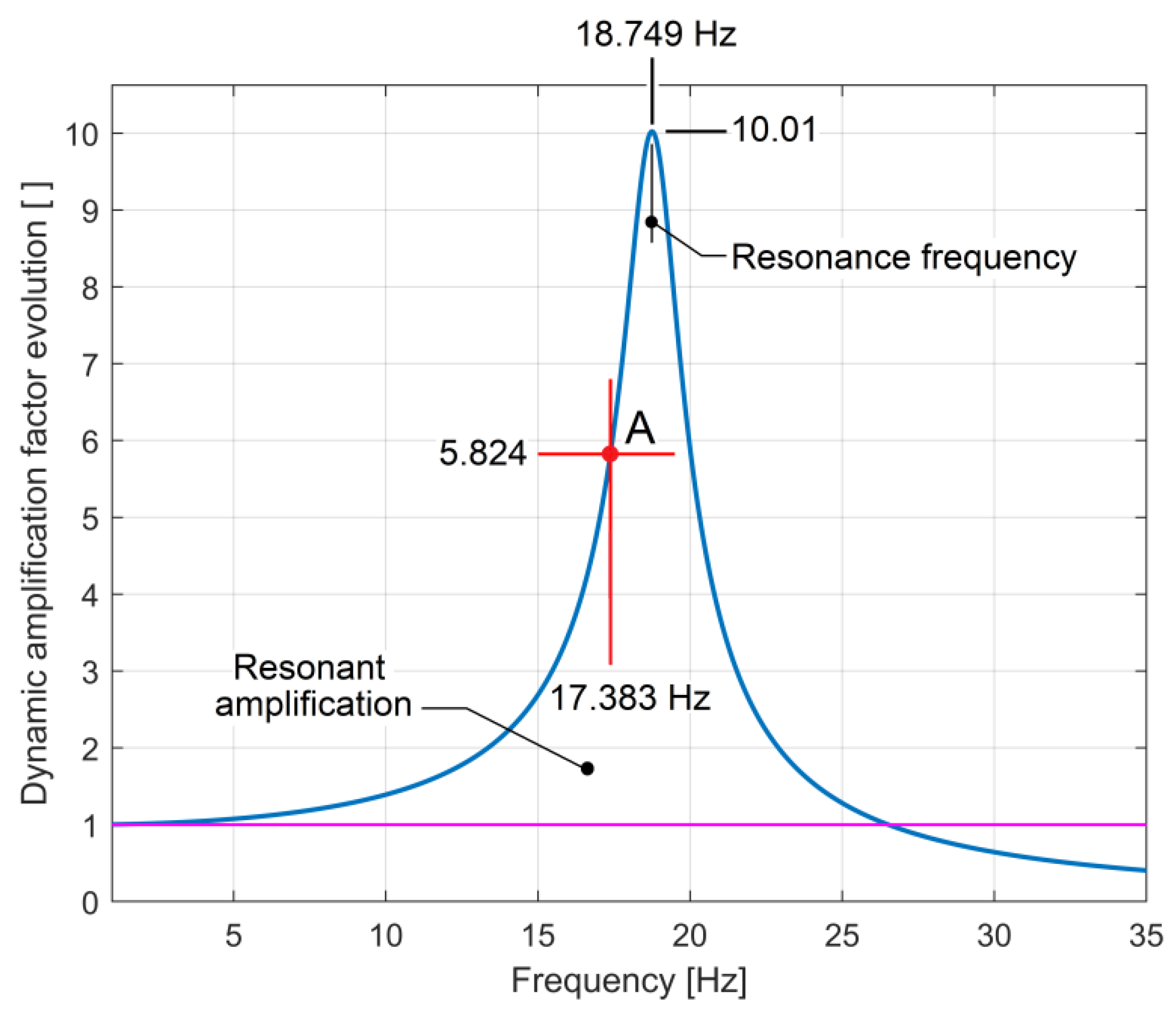
Here ω = 2πf is the angular frequency of harmonic excitation on frequency f. Based on previous experimental results of curve fitting (with b and p values in Equation (10)) Figure 18 presents the simulated evolution of Daf related to the frequency of excitation (1 ÷ 35 Hz range). Because of a low damping constant b, the system presents resonant amplification, with a maximum value Daf = 10.01 on f = 18.749 Hz frequency.
Based on the previous experimentally determined frequencies f1 and f2, with f = f1 = 17.3856 Hz gives the result Daf1 = 5.831 and with f = f2 = 17.3752 Hz (or f = f2 = 17.3959 Hz) the result is Daf2 = 5.803 (or Daf2 = 5.859). For f = = 17.383 Hz (Figure 12) the result is Dafc = 5.824 (the coordinates of point A on Figure 18). This means that, because of mechanical resonance, the vibration amplitude generated by the beating phenomenon of the headstock and the lathe on its foundation (already revealed in Figure 7) is amplified on average by 5.824 times.
Besides the amplification of the vibration, the resonant behaviour also introduces a significant shift of phase γ between the excitation (unbalancing) force and the vibration displacement, theoretically described [45] as depending on ω (and excitation frequency f as well) with the equation:
With the b and p values previously determined, the values of shift of phase calculated for each frequency are: γ1 = 0.5691 rad for f = f1 = 17.3856 Hz and γ2 = 0.5656 rad (or γ2 = 0.5725 rad) for f = f2 = 17.3752 Hz (or f2 = 17.3959 Hz). For f = = 17.383 Hz the result is γc = 0.5682 rad.
The knowledge of both of these resonant characteristics (the value of the dynamic amplification factor Daf and especially the phase shift γ) is important for a next approach of the dynamic balancing of these two shafts placed inside the headstock.
As a general comment, we should mention that the resonance behaviour of this low damped vibratory system—as previously mentioned—is a consequence of the disponibility of this system to absorb modal mechanical energy. The system works as a narrow-band modal energy absorber [46].
5. Conclusions and Future Work
Some specific features of the beating vibration phenomenon discovered on a headstock lathe have been revealed in this paper.
An experimental description (with theoretical approaches based on simulations) of this beating vibration phenomenon with very low beat frequency (1/96.6 Hz) was performed. The beating phenomenon occurs due to the addition of vibrations produced by two unbalanced shafts, rotating with very close instantaneous angular speeds (rotating frequencies), with constructive interference in anti-nodes and destructive interference in nodes.
The absolute velocity signal of vibration beating (delivered by a vibration electro-dynamic sensor placed on the headstock) was converted into a displacement signal. For this purpose, a fully confirmed method of numerical integration (antiderivative calculus), with theoretical and experimental approaches was applied. This method is deduced from the approximation of the formula for the first derivative of displacement, as a backward finite difference [43]). An appropriate technique of correction of this numerical antiderivative calculus method was also introduced (mainly by removing the low frequency displacement signal component generated by numerical integration). Thus, an absolute velocity vibration sensor together with a numerical integration procedure plays the role of an absolute vibration displacement sensor.
A consistent part of the research was focused on the resultant vibration displacement signal, mainly on the evolution of frequency (or the combination frequency fc) related to the nodes and anti-nodes position. It was theoretically discovered (by simulation) and was experimentally proved that, in opposition to the literature reports, the combination frequency is not constant, and the definition of its average value is wrong. The evolution of the combination frequency has a specific periodic pattern (having the same frequency as the beat frequency) with small variation (tens of millihertz) and negative or positive peaks placed in beating nodes. The appearance of these peaks (negative or positive) depends on the relationship between amplitudes and frequencies of vibrations involved in the beating phenomenon. The small variation of frequency inside the pattern and the correlation between the frequencies of different experimental signals (the combination frequency fc, the rotation frequency f1 of the main spindle, and the supply voltage frequency of the driving motor) have been correctly described as a result of a high accuracy procedure of frequency measurement, developed in a previous work [42] and successfully applied here. It was proved on a simulated signal (having a frequency of 17.383 Hz, equal to the average value of the combination frequency in vibration beating phenomenon) that this procedure has less than ±1.5 μHz measurement error.
The influence of the behaviour of the headstock and lathe foundation dynamics (as a rigid body placed on a spring–damper system) on the vibration induced by unbalanced rotors and the beating phenomenon was also investigated. Based on computer-aided analysis of free damped viscous response (by curve fitting), the characteristics of foundation dynamics were experimentally revealed (mainly the values of natural angular frequency and the damping constant). Considering these values, the dynamic amplification factors of vibrations (mainly of the resultant vibration) and phase shift between centrifugal forces (as excitation forces produced by unbalanced rotary shafts) and the vibrations generated by these forces were calculated.
For each experiment, numerical simulation and signal processing procedures, several computer programs written in Matlab were successfully used.
In the future, the theoretical and experimental approaches will be focused on the influence of dynamic unbalancing and vibration beating on the active and instantaneous electrical power absorbed by the driving motor of the headstock. There is a logical reasoning for these approaches: the headstock vibration motion (especially during the resonant amplification behaviour revealed in Figure 18) should be mechanically powered. Of course, the instantaneous and active mechanical power (difficult to measure) is delivered by the driving motor as an equivalent of instantaneous and active electric power absorbed from the electrical supply network (easier to measure).
Several theoretical and experimental studies on computer-aided balancing of each rotary shaft inside the lathe headstock will be performed (using two absolute velocity sensors and an appropriate method of computer-assisted experimental balancing). A study on the vibration beating phenomenon produced by more than two unbalanced rotary bodies will be done.
Author Contributions
Conceptualization, D.-F.C. and M.H.; methodology, D.-F.C. and M.H.; software, F.N. and C.-G.D.; validation, M.H. and C.-G.D.; formal analysis, D.-F.C. and M.H.; investigation, D.-F.C., C.-G.D. and M.H.; resources, M.H.; data curation, M.H.; numerical integration method, M.H.; writing—original draft preparation D.-F.C. and M.H.; writing—review and editing, G.D., M.I.; visualization, M.H. and F.N.; supervision, M.H. and C.-G.D.; project administration, M.H. and C.-G.D.; funding acquisition, D.-F.C., G.D. and M.I. All authors have read and agreed to the published version of the manuscript.
Funding
This work was accomplished with the support of the COMPETE project nr. 9PFE/2018, funded by the Romanian Government.
Acknowledgments
This work was accomplished with the support of COMPETE project nr. 9PFE/2018, funded by the Romanian Government.
Conflicts of Interest
The authors declare no conflict of interest.
Nomenclature
| A1 , A2 | The amplitudes of vibrations y1, y2 [m] |
| ae-bt | The envelope of free viscous damped vibration velocity response [m/s] |
| b | The damping constant [s−1] |
| C | The constant of velocity signal integration [m] |
| Daf | Theoretical dynamic amplification factors of vibrations [ ] |
| Daf1,Daf2 | Dynamic amplification factors of vibrations y1, y2 produced by shafts 1, 2 [ ] |
| Dafc | Dynamic amplification factor of resultant vibration y1 + y2 at average frequency fc [ ] |
| dy1 /dt, dy2 /dt | The derivative of vibration displacements y1, y2 (vibration velocities) [m/s] |
| f | The frequency of harmonic excitation of the lathe headstock [Hz] |
| F1 , F2 | The horizontal projection of the rotary unbalance forces generated by shafts 1 and 2 [N] |
| f1 , f2 | The frequency of vibrations y1, y2 [Hz] |
| fb | The beat frequency [Hz] |
| fc | The frequency of the resultant vibration y1 + y2, or combination frequency [Hz] |
| IAS | Instantaneous angular speed [rad/s] |
| k | The stiffness of headstock and lathe foundation [N/m] |
| m1 , m2 | Unbalance mass on rotary shafts 1, 2 [Kg] |
| n | A natural number involved in the definition of the beat period Tb |
| p | The natural angular frequency [rad/s] |
| p1 | The angular frequency of damped harmonic vibration [rad/s] |
| r1 , r2 | The distance between the center of the unbalance mass and the rotation axis on shafts 1, 2 [m] |
| s | The addition of vibration displacements s = y1 + y2 [m] |
| si, si+1 | Two successive displacement samples of vibration [m] |
| si+h, si+h-1 | Two successive displacement samples of vibration [m] |
| t | Time [s] |
| t0 | The origin of time for the theoretical model of free damped vibration velocity [s] |
| tzcj, tzcj+1 | Two successive zero-crossing moments of the displacement vibration signal involved in frequency measurement [s] |
| Δt | Sampling interval for a numerically described signal [s] |
| T1 , T2 | The periods of vibrations y1, y2 [s] |
| Tb | The beat period, with Tb = 1/fb [s] |
| Tc | The period of the resultant vibration y1 + y2, with Tc = 1/ fc [s] |
| v | The velocity of the resultant vibration in beating [m/s] |
| vfd | The vibration velocity of the headstock during a free damped response [m/s] |
| vi | A sample of the vibration velocity [m/s] |
| y1 , y2 | The vibration displacement generated by shafts 1, 2 [m] |
| y1s , y2s | Simulated vibration displacement signals [m] |
| α | The phase angle at the origin of time t0 for a theoretical model of free damped vibration velocity [rad/s] |
| εf | The error in the frequency measurement [Hz] |
| εj, εj+1 | The calculus errors for two successive zero-crossing moments [s] |
| γ | The shift of phase between the excitation force and the vibration displacement in the free damped response [rad] |
| θ1 , θ2 | The instantaneous value of the angle of centrifugal forces to the horizontal direction [rad] |
| φ1 , φ2 | The values of θ1 and θ2 at the origin of time, t = 0 [rad] |
| ω | The angular frequency of harmonic excitation of the lathe headstock [rad/s] |
| ω1 , ω2 | The instantaneous angular speed of the rotary shafts 1, 2 [rad/s] |
References
- Muszyńska, A. Rotordynamics; CRC Press: Boca Raton, FL, USA, 2005; ISBN 978-0-8247-2399-6. [Google Scholar]
- Wang, Y.; Yuan, X.; Sun, R. Critical techniques of design for large scale centrifugal shakers. World Inf. Earthq. Eng. 2011, 27, 113–123. [Google Scholar]
- Anekar, N. Design and testing of unbalanced mass mechanical vibration exciter. IJRET 2014, 3, 107–112. [Google Scholar]
- Conley, K.; Foyer, A.; Hara, P.; Janik, T.; Reichard, J.; D’Souza, J.; Tamma, C.; Ababei, C. Vibration alert bracelet for notification of the visually and hearing impaired. J. Open Hardw. 2019, 3, 4. [Google Scholar] [CrossRef]
- Fontana, F.; Papetti, S.; Jarvelainen, H.; Avanzini, F. Detection of keyboard vibrations and effects on perceived piano quality. J. Acoust. Soc. Am. 2017, 142, 2953–2967. [Google Scholar] [CrossRef]
- Ippolito, R.; Settineri, L.; Sciamanda, M. Vibration monitoring and classification in centerless grinding. In International Centre for Mechanical Sciences (Courses and Lectures); Kuljanic, E., Ed.; Springer: Vienna, Austria, 1999; p. 406. [Google Scholar] [CrossRef]
- Merino, R.; Barrenetxea, D.; Munoa, J.; Dombovari, Z. Analysis of the beating frequencies in dressing and its effect in surface waviness. CIRP Annal. Manuf. Technol. 2019, 68, 353–356. [Google Scholar] [CrossRef]
- Mayoof, F.N. Beating phenomenon of multi-harmonics defect frequencies in a rolling element bearing: Case study from water pumping station. World Acad. Sci. Eng. Technol. 2009, 57, 327–331. [Google Scholar]
- Pham, M.T.; Kim, J.-M.; Kim, C.H. Accurate bearing fault diagnosis under variable shaft speed using convolutional neural networks and vibration spectrogram. Appl. Sci. 2020, 10, 6385. [Google Scholar] [CrossRef]
- Park, J.; Lee, J.; Ahn, S.; Jeong, W. Reduced ride comfort caused by beating idle vibrations in passenger vehicles. Int. J. Ind. Ergon. 2017, 57, 74–79. [Google Scholar] [CrossRef]
- Huang, P.; Lee, W.B.; Chan, C.Y. Investigation of the effects of spindle unbalance induced error motion on machining accuracy in ultra-precision diamond turning. IJMTM 2015, 94, 48–56. [Google Scholar] [CrossRef]
- Norfield, D. Practical Balancing of Rotating Machinery; Elsevier Science: Amsterdam, The Netherlands, 2005. [Google Scholar]
- Thearle, E.L.; Schenectady, N.Y. Dynamic balancing of rotating machinery in the field. ASME Trans. 1934, 56, 745–775. [Google Scholar]
- Kelm, R.; Kelm, W.; Pavelek, D. Rotor Balancing Tutorial. In Proceedings of the 45th Turbomachinery and 32th Pump Symposia, Houston, TX, USA, 12–16 September 2016. [Google Scholar]
- Wijk, V.; Herder, J.L.; Demeulenaere, B. Comparison of various dynamic balancing principles regarding additional mass and additional inertia. J. Mech. Robot. 2009, 1, 4. [Google Scholar] [CrossRef] [Green Version]
- Isavand, J.; Kasaei, A.; Peplow, A.; Afzali, B.; Shirzadi, E. Comparison of vibration and acoustic responses in a rotary machine balancing process. Appl. Acoust. 2020, 164, 107258. [Google Scholar] [CrossRef]
- Bertoneri, M.; Forte, P. Turbomachinery high speed modal balancing: Modelling and testing of scale rotors. In Proceedings of the 9th IFToMM International Conference on Rotor Dynamics. Mechanisms and Machine Science, Milan, Italy, 22–25 September 2017; Pennacchi, P., Ed.; Springer: Cham, Switzerland, 2017. [Google Scholar] [CrossRef]
- Caoa, H.; Dörgelohb, T.; Riemerb, O.; Brinksmeier, E. Adaptive separation of unbalance vibration in air bearing spindles. Proc. CIRP 2017, 62, 357–362. [Google Scholar] [CrossRef]
- Majewski, T.; Szwedowicz, D.; Melo, M.A.M. Self-balancing system of the disk on an elastic shaft. J. Sound Vib. 2015, 359, 2–20. [Google Scholar] [CrossRef]
- Hashimoto, F.; Gallego, I.; Oliveira, J.F.G.; Barrenetxea, D.; Takahashi, M.; Sakakibara, K.; Stalfelt, H.O.; Staadt, G.; Ogawa, K. Advances in centerless grinding technology. CIRP Annal. 2012, 61, 747–770. [Google Scholar] [CrossRef]
- Zhang, Z.X.; Wang, L.Z.; Jin, Z.J.; Zhang, Q.; Li, X.L. Non-whole beat correlation method for the identification of an unbalance response of a dual-rotor system with a slight rotating speed difference. MSSP 2013, 39, 452–460. [Google Scholar] [CrossRef]
- Zhang, Z.X.; Zhang, Q.; Li, X.L.; Qian, T.L. The whole-beat correlation method for the identification of an unbalance response of a dual-rotor system with a slight rotating speed difference. MSSP 2011, 25, 1667–1673. [Google Scholar] [CrossRef]
- Lee, Y.J. 8.03SC Physics III: Vibrations and Waves. Fall 2016. Massachusetts Institute of Technology: MIT Open CourseWare. 2016. Available online: https://ocw.mit.edu (accessed on 17 September 2020).
- Kim, S.H.; Lee, C.W.; Lee, J.M. Beat characteristics and beat maps of the King Seong-deok Divine Bell. JSV 2005, 281, 21–44. [Google Scholar] [CrossRef]
- Yuan, L.; Järvenpää, V.M. On paper machine roll contact with beating vibrations. Appl. Math. Mech. 2006, 6, 343–344. [Google Scholar] [CrossRef]
- Gao, H.; Meng, X.; Qian, K. The Impact analysis of Beating vibration for active magnetic bearing. IEEE Access 2019, 7, 134104–134112. [Google Scholar] [CrossRef]
- Preumont, A. Twelve lectures on Structural Dynamics; Université Libre de Bruxelles: Brussels, Belgium, 2012. [Google Scholar]
- Horodinca, M.; Seghedin, N.; Carata, E.; Boca, M.; Filipoaia, C.; Chitariu, D. Dynamic characterization of a piezoelectric actuated cantilever beam using energetic parameters. Mech. Adv. Mater. Struct. 2014, 21, 154–164. [Google Scholar] [CrossRef]
- Endo, H.; Suzuki, H. Beating vibration phenomenon of a very large floating structure. J. Mar. Sci. Technol. 2018, 23, 662–677. [Google Scholar] [CrossRef]
- Carrino, S.; Nicassio, F.; Scarselli, G. Subharmonics and beating: A new approach to local defect resonance for bonded single lap joints. J. Sound Vib. 2019, 456, 289–305. [Google Scholar] [CrossRef]
- Cattarius, J.; Inman, D.J. Experimental verification of intelligent fault detection in rotor blades. Int. J. Syst. Sci. 2000, 31, 1375–1379. [Google Scholar] [CrossRef]
- Morrone, A. Seismic vibration testing with sine beats. Nucl. Eng. Des. 1973, 24, 344–356. [Google Scholar] [CrossRef]
- Huang, H.H.; Chen, K.S. Design, analysis, and experimental studies of a novel PVDF–based piezoelectric energy harvester with beating mechanisms. Sens. Actuators A Phys. 2016, 238, 317–328. [Google Scholar] [CrossRef]
- Basovich, S.; Arogeti, S. Identification and robust control for regenerative chatter in internal turning with simultaneous compensation of machining error. Mech. Syst. Sign. Process. 2021, 149, 107208. [Google Scholar] [CrossRef]
- Li, D.; Cao, H.; Liu, J.; Zhang, X.; Chen, X. Milling chatter control based on asymmetric stiffness. Int. J. Mach. Tools Manuf. 2019, 147, 103458. [Google Scholar] [CrossRef]
- Yana, Y.; Xub, J.; Wiercigrochc, M. Influence of work piece imbalance on regenerative and frictional grinding chatters. Proc. IUTAM 2017, 22, 146–153. [Google Scholar] [CrossRef] [Green Version]
- Kimmelmann, M.; Stehle, T. Measuring unbalance-induced vibrations in rotating tools. MATEC Web Conf. 2017, 121, 03012. [Google Scholar] [CrossRef]
- Gohari, M.; Eydi, A.M. Modelling of shaft unbalance: Modelling a multi discs rotor usingK-nearest neighbor and decision tree algorithms. Measurement 2020, 151, 107253. [Google Scholar] [CrossRef]
- Hui, S.; Xiaoqiang, H.; Zhiqiang, D.; Lichang, X.; Haishui, J. Research on Low Frequency Noise Caused by Beat Vibration of Rotary Compressor. In Compressor Engineering Conference, Proceedings of the 24th International Compressor Engineering Conference, Purdue, Italy, 9–12 July 2018; Purdue University: Purdue, Italy, 2018; p. 2528. [Google Scholar]
- Available online: http://hgsindia.com/www.hgsproducts.nl/Pdf/196216HG-4%20V%201.1.pdf (accessed on 17 September 2020).
- Available online: https://www.picotech.com/oscilloscope/4224-4424/picoscope-4224-4424-overview (accessed on 17 September 2020).
- Horodinca, M.; Ciurdea, I.; Chitariu, D.F.; Munteanu, A.; Boca, M. Some approaches on instantaneous angular speed measurement using a two-phase n poles AC generator as sensor. Measurement 2020, 157, 107636. [Google Scholar] [CrossRef]
- Chapra, S.C.; Canale, R.P. Numerical Methods for Engineers, 7th ed.; McGraw Hill Education: New York, NY, USA, 2015. [Google Scholar]
- Arlinghaus, S. Practical Handbook of Curve Fitting, 1st ed.; CRC Press: Boca Raton, FL, USA, 2020. [Google Scholar]
- Shabanna, A.A. Theory of Vibrations. An introduction; Springer: New York, NY, USA, 1991. [Google Scholar]
- Schmitz, T. Modal interactions for spindle, holders, and tools. Proc. Manuf. 2020, 48, 457–465. [Google Scholar] [CrossRef]
Figure 1.
A simulation of the beating phenomenon, where: y1 is the vibration of shaft 1; y2 is the vibration of shaft 2, Tb is the beat period; and Tc is the period of the resultant vibration y1 + y2.
Figure 1.
A simulation of the beating phenomenon, where: y1 is the vibration of shaft 1; y2 is the vibration of shaft 2, Tb is the beat period; and Tc is the period of the resultant vibration y1 + y2.

Figure 2.
(a) A lateral view of the shafts involved in the beating phenomenon (with a flat belt transmission between the shafts); (b) A front view of the lathe headstock with the vibration sensor.
Figure 2.
(a) A lateral view of the shafts involved in the beating phenomenon (with a flat belt transmission between the shafts); (b) A front view of the lathe headstock with the vibration sensor.

Figure 3.
The evolution of the velocity of headstock vibrations with a beating phenomenon due to rotary unbalanced shafts; here Tb is the beat period, A is a label for a future comment on signal evolution.
Figure 3.
The evolution of the velocity of headstock vibrations with a beating phenomenon due to rotary unbalanced shafts; here Tb is the beat period, A is a label for a future comment on signal evolution.

Figure 4.
A zoomed-in detail of Figure 3 in the area labelled as A.
Figure 4.
A zoomed-in detail of Figure 3 in the area labelled as A.

Figure 5.
(a) The result of numerical integration of velocity evolution from Figure 3; and (b) the result of removing the zero-offset influence on numerical integration of velocity from Figure 5a.

Figure 6.
The result of the numerical derivative of the evolution from Figure 5b (vibration velocity, practically similar with Figure 3).

Figure 7.
The headstock vibration displacement evolution during the beating phenomenon, deduced by numerical integration and correction of the signal depicted in Figure 3.
Figure 7.
The headstock vibration displacement evolution during the beating phenomenon, deduced by numerical integration and correction of the signal depicted in Figure 3.

Figure 8.
(a) A detail concerning the evolution of velocity (Figure 3) overlaid on the numerical differentiation of the displacement depicted in Figure 7; and (b) a detail of area A of Figure 7 with Tc, the period of the resultant vibration.

Figure 9.
The evolution of the instantaneous combination frequency fc on the simulated vibration beating during a beat period Tb (with A2 > A1 and f2 > f1).
Figure 9.
The evolution of the instantaneous combination frequency fc on the simulated vibration beating during a beat period Tb (with A2 > A1 and f2 > f1).

Figure 10.
The evolution of the instantaneous combination frequency on simulated vibration beating during a beat period (the same condition as in Figure 9, except for the amplitudes relationship: A1 > A2).
Figure 10.
The evolution of the instantaneous combination frequency on simulated vibration beating during a beat period (the same condition as in Figure 9, except for the amplitudes relationship: A1 > A2).

Figure 11.
The evolution of the instantaneous combination frequency fc during the vibration beating phenomenon (displacement of headstock) described in Figure 7.
Figure 11.
The evolution of the instantaneous combination frequency fc during the vibration beating phenomenon (displacement of headstock) described in Figure 7.

Figure 12.
The evolution of the low pass filtered instantaneous combination frequency fc during the vibration beating phenomenon described in Figure 7 (a low pass filtering of Figure 11).

Figure 13.
Low-pass filtered rotational frequency evolution of the main spindle and supplying voltage frequency evolution of the driving motor.
Figure 13.
Low-pass filtered rotational frequency evolution of the main spindle and supplying voltage frequency evolution of the driving motor.

Figure 14.
The position of negative peaks on the combination frequency (formally represented) relative to the position of nodes on the vibration beating phenomenon.
Figure 14.
The position of negative peaks on the combination frequency (formally represented) relative to the position of nodes on the vibration beating phenomenon.

Figure 15.
The result of a numerical simulation for the evolutions described in Figure 14.
Figure 15.
The result of a numerical simulation for the evolutions described in Figure 14.

Figure 16.
The evolution of the frequency measurement error εf (for a simulated harmonic signal with combination frequency fc = 17.383 Hz) versus the evolution of the first sampling time (t1 = 0÷Δt, or t1 = 0÷ 200 μs) involved in the first zero-crossing time (tzc1) calculus.
Figure 16.
The evolution of the frequency measurement error εf (for a simulated harmonic signal with combination frequency fc = 17.383 Hz) versus the evolution of the first sampling time (t1 = 0÷Δt, or t1 = 0÷ 200 μs) involved in the first zero-crossing time (tzc1) calculus.

Figure 17.
Some experimental results on signal processing related to free damped vibration of headstock after an impulse excitation (with a rubber mallet).
Figure 17.
Some experimental results on signal processing related to free damped vibration of headstock after an impulse excitation (with a rubber mallet).

Figure 18.
The evolution of the dynamic amplification factor Daf generated by the headstock foundation in the resonance area, based on Equation (10) and experimental free damped response analysis.
Figure 18.
The evolution of the dynamic amplification factor Daf generated by the headstock foundation in the resonance area, based on Equation (10) and experimental free damped response analysis.

© 2020 by the authors. Licensee MDPI, Basel, Switzerland. This article is an open access article distributed under the terms and conditions of the Creative Commons Attribution (CC BY) license (http://creativecommons.org/licenses/by/4.0/).
Share and Cite
MDPI and ACS Style
Chitariu, D.-F.; Negoescu, F.; Horodinca, M.; Dumitras, C.-G.; Dogan, G.; Ilhan, M. An Experimental Approach on Beating in Vibration Due to Rotational Unbalance. Appl. Sci. 2020, 10, 6899. https://doi.org/10.3390/app10196899
AMA Style
Chitariu D-F, Negoescu F, Horodinca M, Dumitras C-G, Dogan G, Ilhan M. An Experimental Approach on Beating in Vibration Due to Rotational Unbalance. Applied Sciences. 2020; 10(19):6899. https://doi.org/10.3390/app10196899
Chicago/Turabian StyleChitariu, Dragos-Florin, Florin Negoescu, Mihaita Horodinca, Catalin-Gabriel Dumitras, Gures Dogan, and Mehmet Ilhan. 2020. "An Experimental Approach on Beating in Vibration Due to Rotational Unbalance" Applied Sciences 10, no. 19: 6899. https://doi.org/10.3390/app10196899
Note that from the first issue of 2016, this journal uses article numbers instead of page numbers. See further details here.