A Model Output Deep Learning Method for Grid Temperature Forecasts in Tianjin Area


1
School of Electrical and Information Engineering, Tianjin University, Tianjin 300072, China
2
Joint Laboratory of Intelligent Identification & Nowcasting Service for Convective System, CMA Public Meteorological Service Center, Beijing 100081, China
3
Tianjin Bureau of Meteorology, Tianjin 300074, China
*
Author to whom correspondence should be addressed.
Appl. Sci. 2020, 10(17), 5808; https://doi.org/10.3390/app10175808
Submission received: 25 June 2020
/
Revised: 6 August 2020
/
Accepted: 18 August 2020
/
Published: 22 August 2020
(This article belongs to the Special Issue Applied Artificial Neural Networks)
Abstract
:In weather forecasting, numerical weather prediction (NWP) that is based on physical models requires proper post-processing before it can be applied to actual operations. Therefore, research on intelligent post-processing algorithms has always been an important topic in this field. This paper proposes a model output deep learning (MODL) method for post-processing, which can improve the forecast effect of numerical weather prediction. MODL is an end-to-end post-processing method based on deep convolutional neural network, which directly learns the mapping relationship between the forecast fields output by numerical model and the observation temperature field in order to obtain more accurate temperature forecasts. MODL modifies the existing deep convolution model according to the post-processing problem’s characteristics, thereby improving the performance of the weather forecast. This paper uses The International Grand Global Ensemble (TIGGE) dataset from European Centre for Medium-Range Weather Forecasts (ECMWF) and the observed air temperature of 2 m obtained from Tianjin meteorological station in order to test the post-processing performance of MODL. The MODL method applied to temperature in post-processing is compared with the ECMWF forecast, Model Output Statistics (MOS) methods, and Model Output Machine Learning (MOML) methods. The Root Mean Square Error (RMSE) of the temperature field predicted by MODL and the observed temperature field is smaller than the other models and the accuracy of the temperature difference of 2 °C (Acc) is higher, especially where the prediction time is in the first three days. The lightweight nature of MODL also makes it suitable for most operations.
1. Introduction
In recent years, most of the meteorological forecasting methods are based on numerical weather prediction (NWP). NWP uses the observations to estimate future atmospheric behavior that is based on the current state and mathematical and physical principles [1]. Since the proposal of numerical forecasting models in the early 20th century, numerical forecasting technology has made significant progress with the rapid development of modeling technology [2,3], observation technology [4,5], and computer technology [6,7,8]. Numerical weather prediction has become a crucial part of meteorological forecasting technology.
However, NWP has some inevitable errors, including initial condition error and model error [9]. The quality of the observations, quality of the observational network, and the handling of observation and background information by the data assimilation system (DAS) are different types of initial condition errors which can be estimated through a variety of means. Ma and Bao [10] pointed out that these uncertainties may be related to the grid process. Mu et al. [11] proposed that some uncertainties may be related to the physical and dynamic processes that are missed or not yet discovered by the numerical model. Ensemble forecasting, a universal numerical forecast technique, is widely applied to operational forecasting in order to recompense for the shortcomings of the NWP physical model and estimate the uncertainty of the forecast. The European Centre for Medium-Range Weather Forecasts (ECMWF) and the National Centers for Environmental Prediction (NCEP) have extensively tested such methods and put them into the operations [12,13].
While the growth of initial condition error can be estimated, the growth of model error is more difficult to determine. Therefore, forecasters are still required to interpret and revise the numerical forecasting in combination with their meteorological knowledge and forecasting experience for the forecast area in order to improve the weather forecast’s accuracy before the weather forecast is released [14], which is called weather consultation. As weather forecasting becomes increasingly useful as a guide in different fields, more types of observation data and greater spatiotemporal resolution forecasts are needed. Continuously upgraded observation equipment provides a large amount of historical data to support NWP models. However, the way of manual weather consultation has become a hindrance due to the slow speed and heavy workload. The emergence of intelligent post-processing algorithms provides the possibility to meet the needs of weather forecasting. Hence, suitable post-processing algorithms for weather consultation are needed to help the manual process of weather consultation [15,16,17].
Typical numerical forecast post-processing methods include the frequency matching method, Model Output Statistics (MOS) [18], Anomaly Numerical-correction with Observations (ANO) [19], Bayesian Model Averaging (BMA) [20], the Kalman filter [21,22], and Model Output Machine Learning (MOML) [23]. However, the success of MOS is based on a large amount of accurate historical observation data. Each update of numerical forecasting models will invalidate the previous historical data. The continuous update of numerical forecasting models prevents MOS from collecting a large amount of historical data. The failure to analyze the potential high-dimensional features in the observation data is also a limitation of MOS. The disadvantage of ANO is that they are not likely to predict sudden changes in the forecast error caused by rapid transitions from one weather regime to another though the ANO does not need too much data and it has a lower computational complexity. The assumption of prior probability is the limitation of BMA. Different prior probabilities generally have a greater impact on the results of the BMA method. BMA sometimes returns poor forecast results due to the bad settings of the prior probabilities. The use of MOML to post-process NWP requires the extraction of hidden high-dimensional features in large amounts of historical data which required meteorological knowledge [24]. Cyclone, wind shear, etc. can all be regarded as high-dimensional features extracted through meteorological knowledge, but only professionals can extract them. Therefore, the complex pre-processing that is related to feature engineering is a deficiency of MOML.
The post-processing methods that are mentioned above can be considered as machine learning algorithms. Machine learning algorithms build a mathematical model based on sample data, known as “training data”, in order to make predictions or decisions [25]. In the post-processing, machine learning algorithms build the model based on historical data to map the relationships between forecast field and observation data. As a branch of machine learning methods, deep learning has demonstrated its remarkable capacities and massive potential in many different fields in recent years. The development of deep learning has also promoted the historical process of artificial intelligence because of its extensive application possibilities [26]. Deep learning has made breakthroughs in many fields, especially in computer vision (CV) [27], speech recognition [28], and natural language processing (NLP) [29]. The emergence of deep learning provides a new approach for several meteorological problems. In recent years, many papers have tried to use deep learning to reduce the model error and initial condition error of NWP. For example, Zambrano et al. [30] used a multilayer feedforward neural network in order to predict Chile’s degree of drought in 2018. Hossain et al. [31] used autoencoders to predict temperature and humidity in Nevada. Dupuy et al. [32] implemented convolutional neural networks to the forecasts of cloud cover. Wang et al. [33] trained a deep belief network in the prediction of wind power. However, the above-mentioned deep learning models that are applied to weather forecasting are gradually replaced by the new models due to slow convergence and easy over-fitting in the CV and NLP areas. In addition, these algorithms establish the mapping relationship between the forecast field and a single weather station. The idea of directly establishing a mapping from the forecast area to the observation area, which can be called as end-to-end post-processing, has not been tried.
In this paper, a model output deep learning (MODL) method is proposed while using two state-of-the-art deep learning techniques, namely Three-Dimensional (3D) Fully Convolutional Neural Networks and U-Net Structure, to correct the numerical prediction. Fully Convolutional Neural Networks, recurrent neural networks, and fully connected neural networks are common deep learning methods to solve pixel-level classification and regression problems. A recurrent neural network is difficult to converge because of the complex structure. The fully connected neural network cannot handle large input tensors due to the large number of parameter requirements. When compared with the fully connected neural network and recurrent neural network, the Fully Convolutional Network that was proposed by Long et al. [34] has a better performance on pixel-level regression. Thus, the 3D Fully Convolutional Network (FCN) is widely used to process 3D data. Li et al. [35] used this structure to detect vehicles in the point cloud. Janssens et al. [36] trained a regression 3D FCN automatic segmentation of lumbar vertebrae from CT images. NWP data post-processing includes three dimensions of time and space, so 3D FCN is also suitable for NWP post-processing. Ronneberger, Fischer, and Brox [37] proposed a U-net structure for biomedical image segmentation. U-net codec structure can fuse multi-scale features in the network. Multi-scale and multi-lifecycle meteorological features need to be comprehensively analyzed during the post-processing of NWP. For example, as a weather system with a small scale and short duration, wind shear affects temperature through ascending movement. Extratropical cyclones with an average diameter of 1000 km will cause large-scale weather changes in the area. It is necessary to comprehensively consider weather systems of different scales in post-processing. Therefore, the U-net structure is suitable for solving the multi-space-time scale post-processing problem. Unlike other papers, the MODL model is an end-to-end training model. No additional human intervention is needed in post-processing. Thus, we propose this MODL method for the post-processing of NWP and employ it to forecast 2 m air temperature forecasting in Tianjin area in this paper. Comparison experiments were conducted that showed the significant improvement of our approach as compared to other widely-used post-processing methods.
2. Data and Organization
This section will explain the data sources, data organization forms and problems solved by the experiment in this article. The data used in the experiment, which is recorded as , consists of two parts: numerical model data and observation data. Section 2.1 will introduce the numerical model data used in the experiment. Section 2.2 will introduce the observation data used in the experiment. Section 2.3 will introduce the problems solved by the experiment in this paper.
2.1. Model Data
Many countries and regions have their own global numerical weather prediction centers, including ECMWF (European Centre for Medium-Range Weather Forecasts), GFS (United States Global Forecast System), or RHMC (Russian Hydrological and Meteorological Center). Among these centers, ECMWF is an independent intergovernmental organization with the world’s largest archive of numerical weather prediction data. Because of the noticeable correction effect on the deterministic forecast of extreme weather, it has become a vital reference product for short- and medium-term weather forecasting [38].
The forecast data that are used in this paper are The International Grand Global Ensemble (TIGGE) dataset, which is the global ensemble forecast data from ECMWF. The model data provided by TIGGE includes wind speed, temperature, precipitation, humidity, and other basic physical quantities and basic weather phenomenon elements that explain the state of the atmosphere, which we call weather elements. During weather consultation, meteorologists will select some, but not all, weather elements for weather consultation based on meteorological principles and their own local forecasting experience. Based on the experience of weather forecasters, this paper selects 21 kinds of weather elements with a correlation with temperature. In the correlation analysis in Section 3, further screening of these weather elements will be carried out.
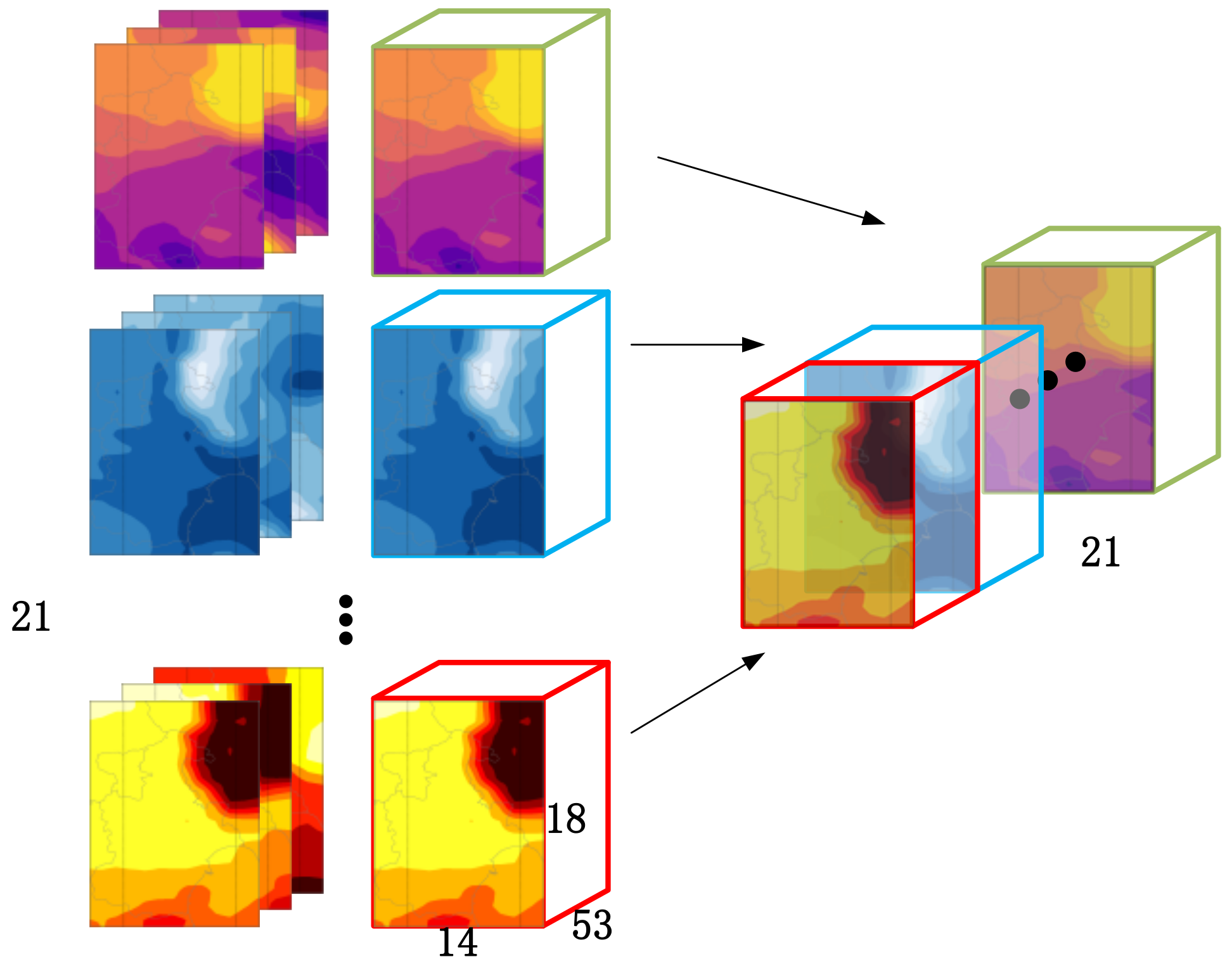
As part of the experimental data , the model forecast data is recorded as . used in the experiment is the combination of three-hourly forecast data initialized at 0000 UTC up to a lead time of 72 h and six-hourly forecast data up to lead time of 240 h from January 2016 to November 2018 provided by Tianjin Bureau of Meteorology. Each day provides a forecast sample from January 2016 to November 2018. Thus, there are 1065 samples recorded as in a specific space on a certain day, i.e., . For the numerical forecast in the above time range with a resolution of 0.125°, the grid shape covering the Tianjin area (38.5°–40.25° N, 116.25°–118.5° E) is 16 × 12. Because grid points at the grid boundary need to be considered, this paper uses grid data with a shape of 18 × 14. Each point on the grid can be represented by (m, n), where and . As part of the experimental data , the model forecast data are recorded as . Each sample contains 21 weather elements and we use to represent some element, i.e., , which will be introduced in detail later. Each sample has 53 time steps (or called forecast lead time) and can be divided into two groups according to the time steps, which is the 3-h interval sample of the first 72 h and the 6-h interval sample of 72–240 h (t = 0, 3, …, 69, 72, 78, …, 234, 240). Each point on the grid can be represented by (m, n), where and . Therefore, the five-dimensional (5D) tensor of size 14 × 18 × 53 × 21 × 1065 can be written as
where is the value of forecast sample with the weather element in grid point whose forecast lead time is .
Figure 1 shows an element in . Three of 21 different weather elements () with fixed parameters are drawn using four different color tables. Each weather element is composed of three heat maps, representing three different time parameters (t). The length of the time dimension is 53, and each time parameter corresponds to a two-dimensional matrix of 14 × 18 in space. The figure shows the value of weather elements in the form of heat maps through nearest neighbor interpolation.
2.2. Observational Data
The observational data are the 2 m air temperature observation data of all 267 automatic stations in Tianjin provided by the Tianjin Meteorological Bureau. Each automatic station recorded the 2 m air temperature of its location hour by hour from January 2016 to November 2018. Thus, these observational data constitute the other part of the original dataset , and this part is denoted by
where the ranges of values of and are , and . Because the maximum forecast lead time of model data is 10 days, each model sample requires 10 days of observation samples as the label of the model input. The EC data eliminated due to the lack of observation data is calculated for a total of 33 days. Accordingly, the time dimension parameter of the numerical forecast data is specifically compressed to 1032.
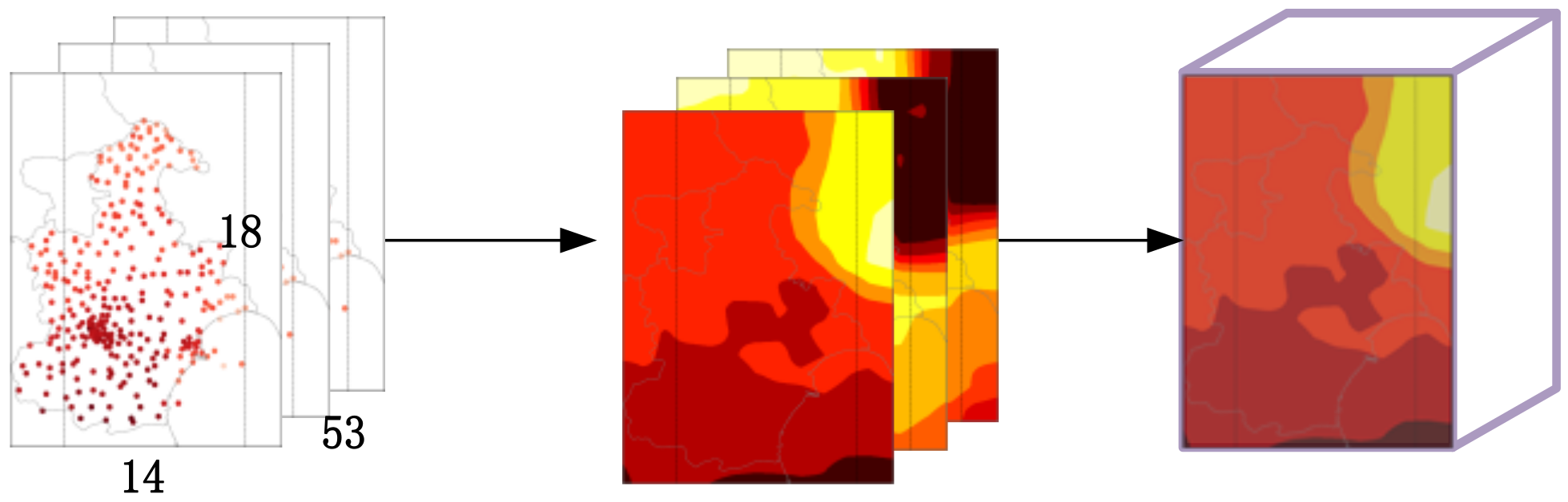
Because the automatic station data is not grid data in space, this paper uses inverse distance interpolation to obtain grid format observation data, as shown in Figure 2. Observation data of 267 automatic stations at 53 time steps are interpolated to form one data for supervision. Inverse distance weighting is the general term for a series of weighted average interpolation methods. Different strategies for setting weights will make some difference in the grid data after interpolation. This paper uses the Cressman strategy [39]. The Cressman strategy uses the ratio between distance of an observation from a grid cell and the maximum allowable distance in order to calculate the relative importance of an observation for calculating an interpolation value.
2.3. Problem
The problem studied in this paper, the grid temperature forecast, is actually a problem of using the forecasts from the ECMWF model as the input and obtaining the 2 m air temperature forecasts, as the output which can be written as
Focusing on the samples from January 2016 to December 2018, for each sample, the 2 m air temperature forecasts in Tianjin area at the forecast lead times of 1–10 days need to be forecast. This paper uses 2 °C temperature difference accuracy (Acc) and root mean square error (RMSE) in order to assess the quality of 2 m air temperature predictions.
This paper trains the MOS method based on univariate linear model, the MOML method based on linear regression model, and the MOML method based on random forest as comparison models in order to examine the advantages and disadvantages of MODL in the numerical prediction post-processing technology. The comparison models of this paper will be introduced in detail in Section 3.3.
3. Methods
This section will introduce the algorithm and usage of the MODL algorithm. MODL is a post-processing algorithm for numerical weather prediction. Like MOS, MODL is also a technology that is used to improve the prediction capabilities of numerical weather models. The difference is that MODL uses the back-propagation capability of the neural network to establish the mapping relationship between NWP and observation data. In addition, the post-processing model established by MODL is an end-to-end model that considers spatio-temporal correlation. Using MODL to post-process, the numerical prediction can make the prediction of meteorological elements more accurate. Section 3.1 will introduce the preprocessing method before model data is input into MODL. Section 3.2 will introduce the training method, operational method and the structure of MODL. Section 3.3 will introduce comparison algorithms.
3.1. Data Preprocessing
Twenty-one kinds of weather elements were selected that may not have strong correlations with temperature forecasts. Weather elements that are less dependent on 2 m air temperature will increase the difficulty of the deep learning model’s convergence and will also affect the forecasting effect of the convergence model [40,41,42]. This paper uses the random forest for the feature selection.
The random forest algorithm is one of the most important machine learning algorithms [43]. It usually has good prediction performance, lower overfitting, and stronger interpretability. In addition to being used as a classifier, random forest can also be used as a tool for feature selection. The random forest consists of a number of flowchart-like structural classifiers called decision trees. Each node of the decision tree will select a feature to classify the input data. These operations will produce many different conditions of the samples. Each condition is evaluated by some kind of indicator, or called loss. The indicator is mean squared error in regression. The temperature prediction problem that is studied in this paper is a typical regression problem, so the mean squared error is used to measure random forest regression. The changes in features affect the loss of the model. For a certain feature, random forest judges the importance of the feature by adding noise to the feature. The greater the loss of the model, the more important the features after adding noise.
Among the 21 weather elements in the numerical model data, the correlation between the 2 m air temperature and observed temperature is much higher than the correlations between other weather elements and the observed temperature. Thus, the 2 m air temperature is removed when selecting features. In the experiment, different parameters will affect the effect of training. Therefore, it is necessary to perform a grid search on the parameters. Grid-search is used to find the optimal hyperparameters of a model, which results in the most ‘accurate’ predictions. However, a lot of calculation time will be wasted if the scope of the grid search is not restricted. Therefore, according to the sample feature dimension and sample size, we set the scope of grid search. The parameters participating in the grid search are “The number of trees in the forest (n_estimators)”, “The maximum depth of the tree (max_depth)”, “The minimum number of samples required to be at a leaf node (min_samples_leaf), and “The number of features to consider when looking for the best split (max_features)”. Table 1 shows the combination range of parameters. The score of the random forest model is obtained by out-of-bag (OOB) score. OOB is the mean prediction score on each training sample , using only the trees that did not have in their bootstrap sample. The higher the OOB score, the stronger the feature selection ability of the model corresponding to the parameter combination.
In the optimal random forest model, essential weather elements are selected as input to the MODL according to the feature correlation score that is calculated by random forest. The feature correlation score here is a score that evaluates the correlation between different weather elements and the observed temperature. Table 2 shows the names of 21 types of weather elements, abbreviations of numerical forecasts, and correlation scores.
The largest correlation in Table 2 is the 925 hPa temperature field, the correlation is 14.43%. Six kinds of elements’ correlation are almost greater than 60%, which are 10-m V wind component (10v), 10-m U wind component (10u), temperature at 850 hPa (t-850), temperature at 925 hPa (t-925), visibility (vis), and mean sea level pressure (msl). Adding the 2 m air temperature, seven of 21 weather elements will be input into MODL after feature selection.
3.2. MODL Method
The core of the MODL is 3D Fully Convolutional Neural Networks (3D FCNN). Acknowledged convolution neural networks (CNN) architectures (such as AlexNet [44] or GoogLeNet [45]) require a fixed-size input image and they use a pooling layer to gradually reduce the spatial resolution of the representation. The spatial knowledge of the features will be completely lost due to the classifier’s fully connected layer. Although the sliding window method can be used to solve the above problems, many redundant convolution operations affect the running speed of the model. Unlike traditional CNNs, FCNNs only consist of convolutional layers, which can be applied to images of any size. Because the spatial graphs of class scores are obtained in a single dense inference step, FCNN can avoid redundant convolution and pooling operations, thereby making them more computationally efficient. The post-processing of temperature prediction is greatly affected by spatial information. NWP data are also grid data in units of time and space. The size of the model input space is uncertain when the model is applied in other regions. Therefore, the structure of the FCNN is more suitable for the MODL model.
The 3D FCNN is composed of three convolutional layers, and each convolutional layer is composed of several 7 × 7 × 7 convolution kernels. The output of each convolutional layer is noted as the feature map. The k-th output of the l-th convolutional layer can be written as:
where is the number of the convolution kernels in layer l of the network, is the n-th input of the l-th layer convolution, is the kernel convolved with the previous output features, is the bias, and f is a non-linear activation function. The feature map that is generated by convolution is slightly smaller than its input volume. The output feature map will be two pixels smaller in each dimension than the input feature map. For a convolution kernel of size 3 × 3 × 3, each convolution operation will reduce 2 units on the space-time scale of the output tensor. In order to make the output tensor the same size as the input tensor, three solutions have been used to compare. The first one is to use bilinear interpolation to reduce output tensor after each convolution to the same size as the input tensor. The second is to choose a larger input area as MODL input, which can be calculated by the number of convolution modules and the size of convolution kernel. The last one is to use the boundary expansion method to appropriately expand the boundary size of the input tensor. The experiments show that effects of the three methods above are very close, so that the experiments discussed in this paper use the neighbor value filling method to deal with the boundary effect.
Therefore, MODL is a multi-layer network structure with the above-mentioned convolutional layer as the basic unit. The parameters of the convolutional layer are updated by training MODL. In operations, the trained MODL can post-process the numerical weather prediction data to obtain more accurate prediction results. Section 3.2.1 will introduce the training and operational process of MODL. Section 3.2.2 will introduce the structure of MODL.
3.2.1. The Training and Operational Process of MODL
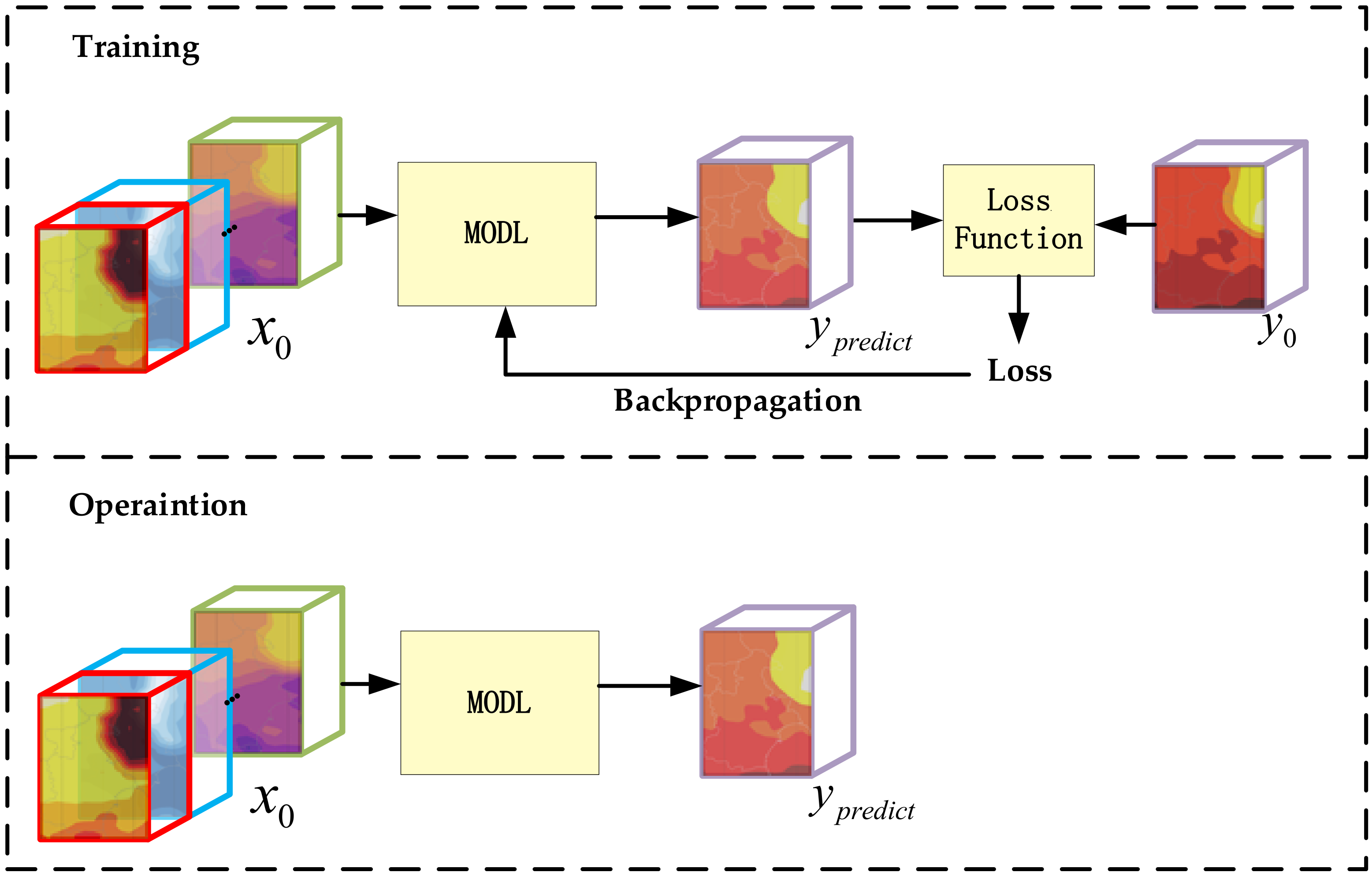
This subsection will describe the training and operational process of MODL. Figure 3 shows the flow chart. The convolution parameters of MODL can be changed while training the model. However, the parameters of MODL are fixed during the operations.
The model requires model data () and observation data () during training. The MODL processing model data with random initialization parameters obtain the forecast tensor, which is noted as . The difference between the predicted tensor and the observed data can be calculated through a custom loss function. The loss function used in this paper’s experiment is the mean square error. The parameters of MODL are updated through gradient backpropagation after each loss is obtained. The trained MODL is the model that is saved by repeating the above operations until the loss is no longer reduced.
In the operations, the parameters of MODL are fixed and the value of the parameters is set by the training process. MODL directly processes model data to get the forecast tensor. When compared with using model data as the forecast result, the forecast result output by MODL is closer to the real observation data.
3.2.2. The Structure of MODL
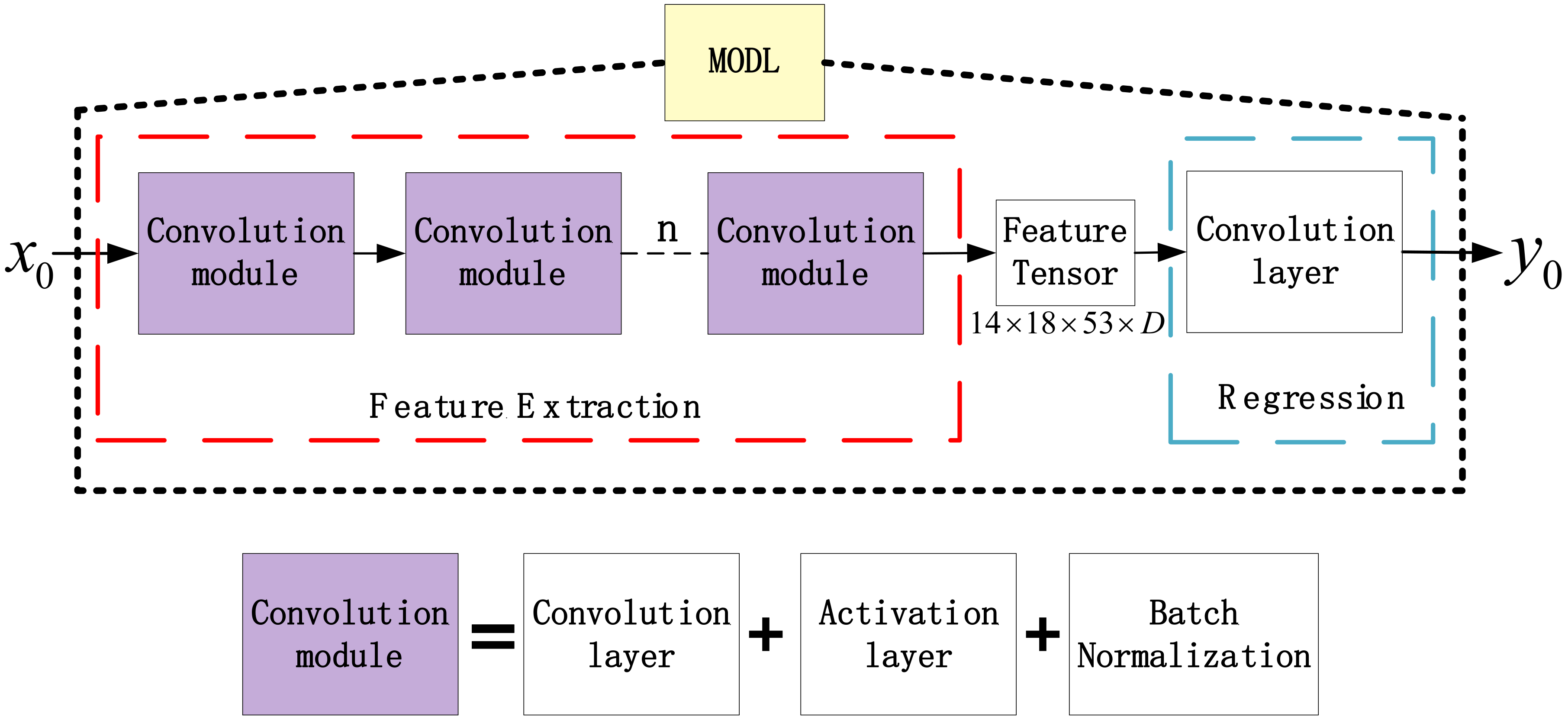
This subsection will describe the structure of MODL. Figure 3 shows the base framework. The post-processing method based on the MODL model can be summarized as two tasks, i.e., high-dimensional feature extraction and regression. The feature extraction part uses different convolution kernels to process input data. The high-dimensional feature tensors will be extracted through the convolution operation in a specific spatiotemporal range, which can get different spatiotemporal information nonlinearly. The regression part uses the convolution kernel of size 1 × 1 × 1 to integrate a single coordinate with different feature capabilities for regression. The shape of the data after data preprocessing is 14 × 18 × 53 × 7. Assume that the number of features extracted for each pixel is D, the shape of the feature tensor after high-dimensional feature extraction is 14 × 18 × 53 × D. The shape of the prediction result by the regression module is 14 × 18 × 53, which corresponds to the prediction results’ 53 time steps and the grid space of the 18 × 14 range.
The purple module is the convolution module, as shown in Figure 4. In addition to the convolution layers, the convolution modules also have regularization layers and activation layers. The feature extraction part is composed of multiple convolution modules. The number of convolution modules is affected by the spatial and temporal scale of the processed data. According to the different number of convolutional modules in feature extraction, this paper builds two MODL architectures, namely 3D Fully Convolutional Neural Network Model (MODL-PLAIN) and 3D Fully Convolutional Neural Network Model Based on U-Net Structure (MODL-U). MODL-PLAIN, with three convolutional modules, and MODL-U, with five convolutional modules, pooling and deconvolution operations, will be described in detail in the rest of this subsection.
3D Fully Convolutional Neural Network Model (MODL-PLAIN)
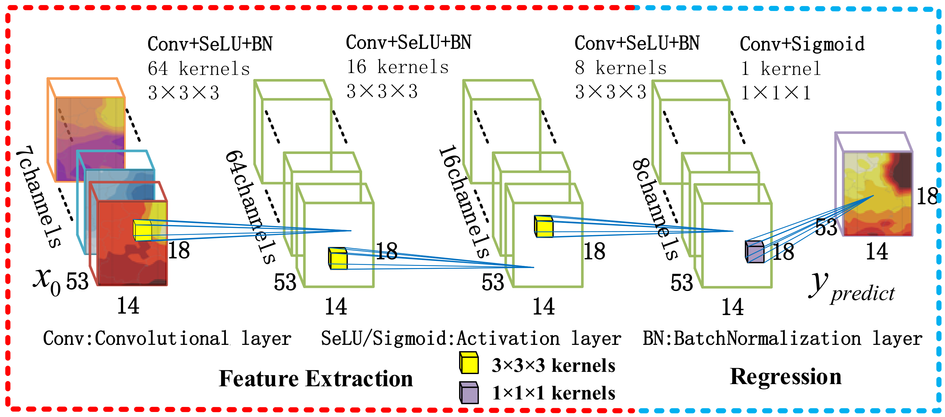
The proposed MODL-PLAIN conducts post-processing using a stack of locally connected convolutional layers. Figure 5 shows the model structure. The low-level convolution in the red dotted frame on the left is used for general feature extraction. The high-level convolution in the blue dotted frame on the right uses these features to regress temperature predictions.
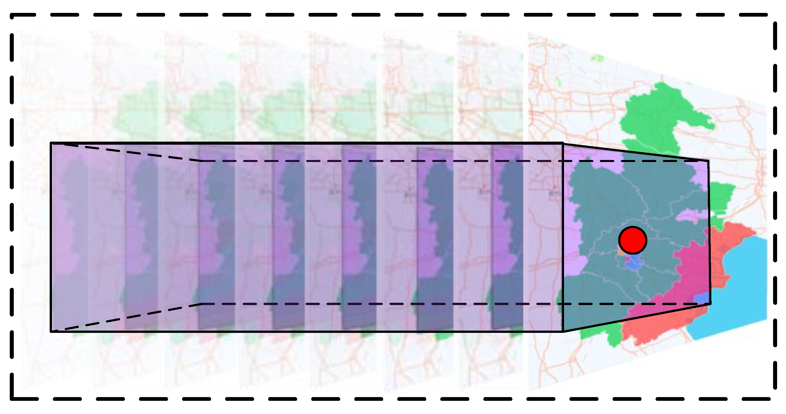
The feature extraction part of MODL-PLAIN is composed of three convolution modules. For the problem examined in this paper, the scale of the convolution kernel is set to . The feature extraction part can integrate a square area with a length of eight pixels pitch with the output pixel as the center point in space and time information with eight-time intervals around the output time point as the center. Figure 6 uses a geographical location in Tianjin as an example to visualize the impact of feature extraction. The location of the red dot, which is the center of the forecast area on each map, in the figure is . The information that MODL-PLAIN can integrate is the purple part of the picture, which contains 80% of Tianjin area. In the longitude direction, it can include an area of 172 km from the output point in the east-west direction. On the other hand, the information of the area of 222 km from the output point in the north-south direction can be included in the latitude direction. Therefore, the model can find the relationship between the output points of the numerical forecast over a large spatial range at the same time dimension. In the time direction, the 3-h interval model can be fully considered by the temperature change of one day before and after the output grid (3 h × 8 = 24 h). The temperature change of two days before and after the output grid (6 h × 8 = 48 h) can be fully considered by the 6-h interval model.
For the activation function, we used Scale Exponential Linear Unit (SeLU) [46] instead of the popular Rectified Linear Unit (ReLU) [47]. This function can be formulated as
where the x defines the input signal, represents the output of the activation function, and is a scaling coefficient for when x is negative. This activation function can modify the rectifier to its input, improving the accuracy of the network with a few extra calculation costs. ReLU directly sets the inputs to zero, while SeLU obtains the parameter a by calculation, so that the network has the ability to be self-normalization.
Although SeLU has provided the convolution module with regularization capabilities, the additional regularization module [48] can still improve the regression effect of the model. Therefore, each convolution module in the feature extraction part on the left side of the figure adds a regularization operation.
3D Fully Convolutional Neural Network Model Based on U-Net Structure (MODL-U)
The convolution structure of MODL-PLAIN can integrate the spatiotemporal information in a certain range. Therefore, the feature tensors that are extracted by the middle-hidden layer are considered to have the same effect as the weather system of different scales. This characteristic tensor that affects temperature prediction is called weather-like system in this paper. Similarly, during weather consultation, meteorologists also analyze the multi-scale weather system extracted from different element fields in order to determine the effect of different elements on temperature forecasting.
Generally, the temperature of a certain area is affected by weather systems of different sizes at the same time. For example, the damp-heat summer in South China is affected by both the large-scale system such as subtropical high and the small-scale system such as wind shear. In addition, due to different life cycles of different weather systems, different life stages (generation, evolution, extinction) of the same weather system have different impacts on weather elements at the same location in the time dimension. Cold fronts and cyclones of different sizes may cause a decrease in temperature. Cold vortex with long life cycle will also cause temperature drop. Therefore, it is necessary to consider the scale of time and space when designing the model.
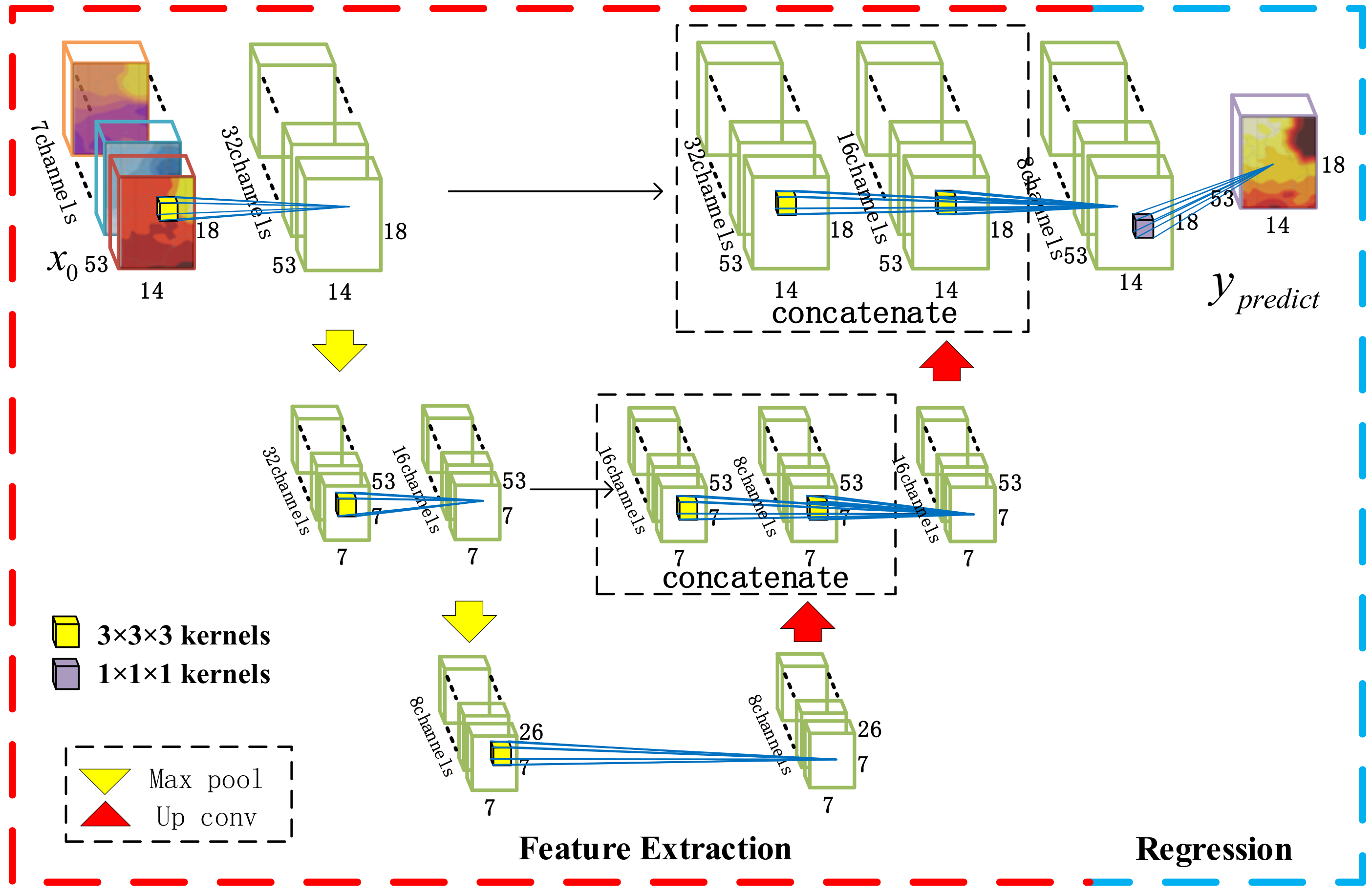
However, the hidden layer features of MODL-PLAIN have the same scale. Weather-like systems of different sizes and different life cycles cannot be extracted. Therefore, this paper proposes a 3D Fully Convolutional Neural Network model that is based on U-Net Structure (MODL-U). The U-net structure is a multi-scale feature fusion method commonly used in the field of computer vision. It uses convolution kernels of the same size to perform a convolution operation on the same feature tensor scaled to different sizes. It is a multi-scale feature fusion parallel branch structure without adding redundant network parameters. Figure 7 shows the MODL-U structure used in this experiment.
The feature extraction of the MODL-U contains five sets of convolution modules and interspersed with two sets of up and downsampling operations in the middle of the convolution modules. Spatial downsampling is to increase the receptive field of the convolution kernel in the spatial range in order to capture more extensive weather-like system characteristics. The temporal downsampling is used to increase the time’s receptive field of the convolution kernel to capture weather-like system information with a longer life cycle. The model can have the ability to process multi-scale information at the same time after upsampling small-scale features and splicing with large-scale features, and then performing convolution operations. Therefore, through the scale transformation of the space-time dimension, the characteristics of weather-like systems of different scales are integrated together. The middle layer output of MODL-U has three different shape feature maps. Among them, the feature maps with shape are weather-like system features with smaller scales and shorter life cycles. The feature maps with shape are weather-like system features with large or medium scales and shorter life cycles. The feature maps with shape are weather-like system features with large or medium scales and longer life cycles.
The weather-like system information that is extracted by the convolution kernel is not similar in structure to the weather system in meteorology but has similarities in function. Additionally, it is associated with the division of the training data set, so that multi-fold cross-validation must be used to ensure the effectiveness of the model.
3.3. Comparison Algorithm
3.3.1. MOS Algorithm
Univariate linear MOS, unary linear regression in other words, is one of the most important and widely used statistical post-processing methods. MOS is unary linear regression; thus, only one predictor is needed. The general unary linear regression equation of univariate linear MOS can be written as
where is the predicted value from post-processing, is the output of the NWP model, which is the unprocessed data, and are the slope and intercept of the linear regression equation. The value of the parameter pair of the univariate linear MOS should minimize the temperature difference between the predicted temperature and the observed temperature in a large amount of historical data. The forecast value for different time and space is calculated by its corresponding .
3.3.2. MOML Algorithm
MOML is a machine learning-based post-processing method. It also contains two structures, feature extraction and regression, the same as MODL. The difference is that the feature extraction part needs to be designed with meteorological knowledge, and the regression can be selected from various machine learning models. This paper selects two different MOML algorithms that are based on different kernels as the comparative experiment. One is the linear regression and the other one is the random forest.
Multiple linear regression attempts to model the correlation between two or more analytical features and a response variable by fitting a linear equation to observed data, which can be written as
where is the output of the feature engineering; are the characteristic coefficients obtained by training with observational data that are obtained by the model training. The aim of learning in the training set is to decide the coefficient and , so as to make the result as close to as possible.
Random forest has already been introduced in Section 3.1. The bagging decision tree algorithm is an ensemble of decision trees trained in parallel, and the random forest algorithm is an extended version of the bagging decision tree algorithm, which introduces random attribute selection in the training process of the decision tree.
The MOS algorithm of the univariate linear model, the MOML algorithm that is based on multiple linear regression and the MOML algorithm based on random forest are used as the three comparative experiments in this article. The same training and testing dataset as the MODL algorithm are used to carry out three-dimensional space-time temperature prediction in Tianjin area. The results of the comparison will be discussed in detail in Section 4.
4. Results and Discussion
In this section, the experimental results will be discussed in detail, including the comparison between the different MODL algorithms and the comparison between MODL, MOS, MOML, and the original NWP results. The root-mean-square error (RMSE) and temperature prediction accuracy (Acc) are used to test the results of these algorithms in order to evaluate the effect of these methods on the forecast.
The RMSE is a general evaluation metric for solving regression problems. The RMSE of temperature is denoted by the following
where is the deep learning regression model, is the total number of samples of dataset, is the input, and is the label.
Accuracy is an evaluation indicator for evaluating classification tasks. However, the regression results can be classified into two categories by setting a threshold () for the temperature difference. Accordingly, the accuracy can be used as an indicator to evaluate the temperature regression problem which denoted as . The positive samples are the samples with temperature difference , and negative samples have the temperature difference on the contrary. According to [35], Li et al. choose 2 °C as the threshold of the temperature in Beijing area. Tianjin and Beijing have similar climate characteristics due to the geographical proximity. in this paper is defined as the percentage of absolute deviation of the temperature forecast not being greater than 2 °C, which is formularized as.
where is the number of the samples in which the difference between the forecast temperature and the observational temperature does not exceed ±2 °C and is the negative samples. To prevent confusion, we specifically point out that the calculation of RMSE involves all data and it has no relationships with the threshold.
4.1. Data Organization Scheme
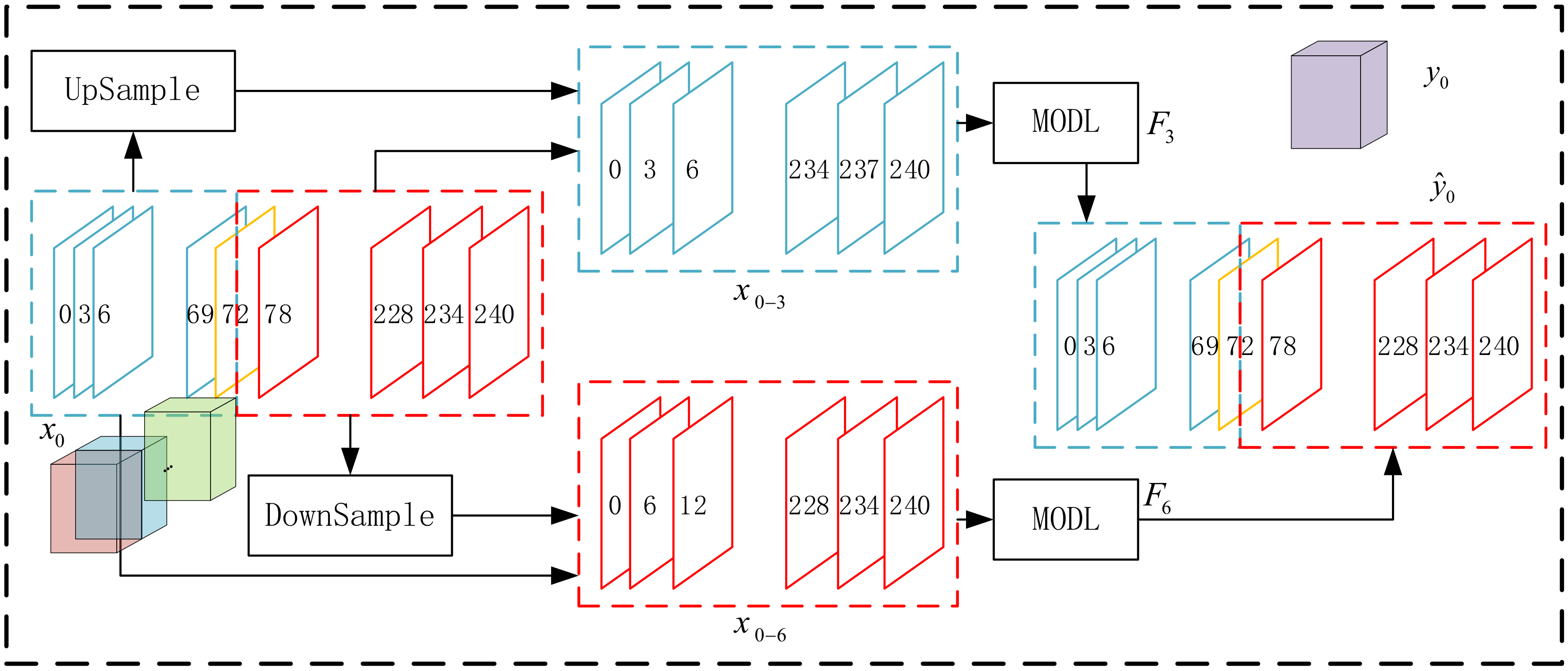
In particular, using one deep learning model to fit may cause inconsistency in time scale, since the mid-term forecast data includes two different time scales, namely, a 3-h interval forecast within 72 h of the reporting time and a 6-h interval forecast within 72–240 h from the reporting times. Accordingly, this paper organizes in the way shown in Figure 8.
For each input tensor , the size is 14 × 18 × 53 × 7. The weather element dimension of the input tensor is omitted in the figure in order to simplify the description. In the time dimension, there are two scales of 3 h (blue part in the figure) and 6 h (red part in the figure). Up-sampling the red part at a 3-h interval and combining the blue part results in a tensor with a time interval of 3 and a size of 14 × 18 × 80 × 7. Down-sampling the blue part at a 6-h interval and combining the red part results in a tensor with a time interval of 6 and a size of 14 × 18 × 40 × 7. Processing the and separately from the two sets of independent models and . Combine the first 24 data presented in the time dimension (the part within 72 h from the reporting time) and the last 29 data in the time dimension (the part that is 72–240 h from the reporting time) into a size of 14 × 18 × 53 as the final forecast result.
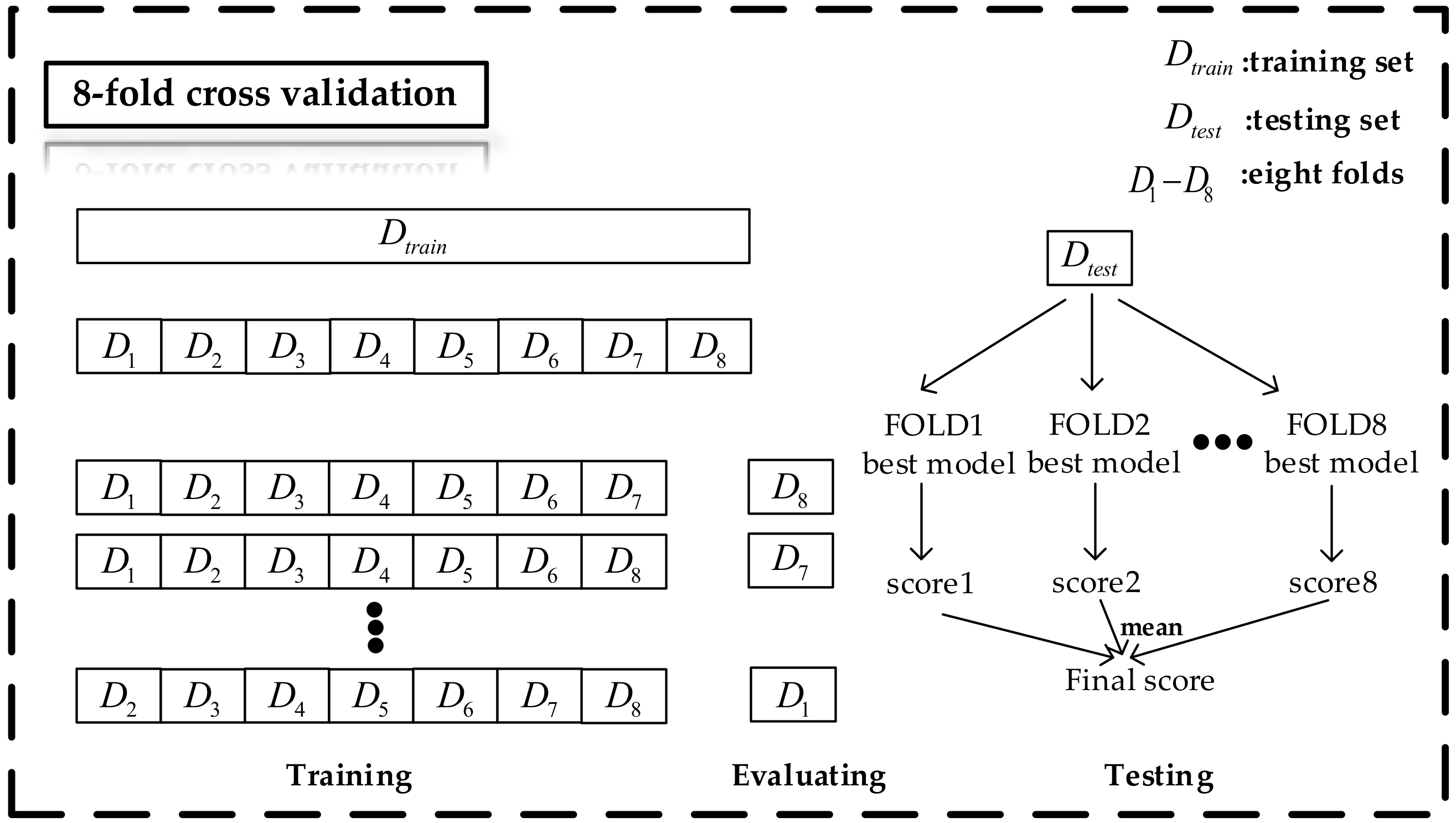
The training is based on eight-fold cross-validation because the massive parameters of deep learning may cause the risk of overfitting the model. The process of training the model can be regarded as selecting a group of suitable hyperparameters to train the model so that the model has a lower forecast error and a higher accuracy rate after training. Each group of hyperparameters corresponds to a score, which can be RMSE or Acc. The training data () is divided into eight folds (), and one part is taken as a validating set each time, and the remaining seven parts are used as the training set. For a group of hyperparameter, use this group of hyperparameters to train the model on seven folds of the training set. The model with the highest score on the validation set (the remaining one-fold) is saved as the optimal model for this fold. The same test data () were input into eight optimal models for evaluation. The mean value of the evaluation score is regarded as the best score of the current hyperparameters. Figure 9 shows the specific process.
4.2. Comparison of MODL, MOML, MOS and EC Forecast
In this subsection, a comparison in the test dataset of the ECMWF model (EC), univariate linear running training period MOS (MOS), MOML, and MODL is presented. The results of MOML with multiple linear regression (MOML-LR), the results of MOML with random forest (MOML-RF), the results of MODL based 3D FCNN (MODL-PLAIN), and the results of MODL based U-structure (MODL-U) are reported.
The more obvious the statistical characteristics of the model data, the better the forecast results. The forecast is negatively correlated with the accuracy. The lower means higher forecast accuracy.
The total number of samples in the test set is 1032 × 0.2 ≈ 206. Each test sample will predict a total of 53 steps in the next 10 days. Each time step has 18 × 14 grid points, and each grid point is regarded as a forecast result. First of all, calculate the and of all the grid data in all time steps of all test samples. The that are shown in Table 3 are the mean value of all forecast grid evaluations of the test set data. It can be seen that using EC data to predict temperature directly has a massive error. All of the post-processing methods have the ability to revise the 2 m air temperature data of the ECMWF model quite fit in the sense of the annual average. MOS can slightly reduce the temperature prediction error. Both MOML models can better improve numerical prediction indicators. The post-processing effect of MODL-PLAIN and MODL-U proposed in this paper is better than other models. MODL-U can reduce the EC forecast error by nearly half.
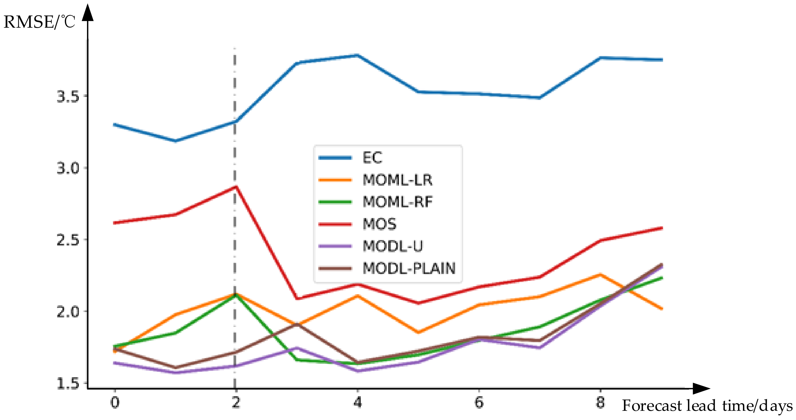
The lead time between the forecast step and the forecast time will affect the final effect of the weather consultation. Therefore, we separately calculate the of all test samples at different time steps and visualize them in Figure 10. The horizontal axis is the forecast lead time, and the vertical axis is . A test sample has 53 grid predictions. Figure 10 shows daily . The time interval for grid forecasting from 0–2 days (left side of the dotted line in the figure) to the reporting time is 3 h, and the time interval of 3–10 days (right side of the dotted line in the figure) is 6 h. The EC forecast error increases nonlinearly with the increase of forecast lead time. The forecasting effect of the first three days is obviously better than 3–10 days. The MOS algorithm can slightly reduce the forecast error of the first three days and greatly reduce the forecast error of 3–10 days. However, generally, in weather consultation, the forecast results of the first three days are more important. Both MOML and MODL algorithms can greatly reduce the daily forecast errors. The MOML algorithm can limit the daily forecast error to about 2 °C. The MOML algorithm based on random forest is slightly better than the MOML algorithm that is based on multiple linear regression. Besides, the error curve of MOML does not increase significantly with the increase in forecast lead time. The MODL-PLAIN algorithm’s improvement effect in the first three days is superior to the MOML algorithm, but the improvement effect of 3–10 days is close to that of MOML-RF. The daily forecast effect of the MODL-U algorithm is the best among all algorithms. Nevertheless, the forecasting time of 72–96 h and 216–240 h is not as good as MOML-RF. These two steps are the left and right boundaries in the time dimension of the 6-h interval model. Therefore, a better algorithm to solve the boundary problem may be needed to improve this result.
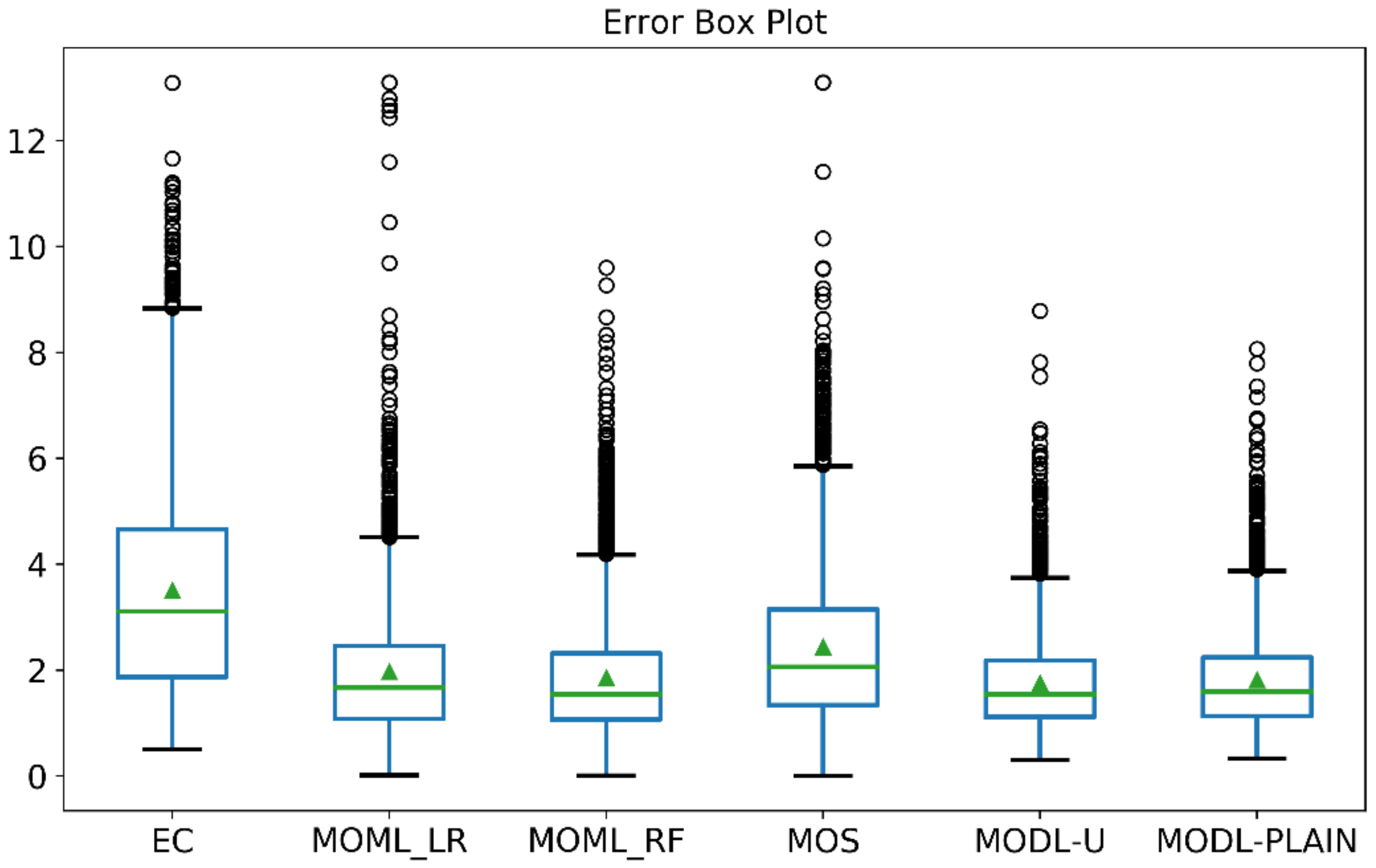
By comparing Table 3 and Figure 10, it is found that the daily in MOML algorithm and MODL algorithm in Figure 10 looks smaller than the total in Table 3. It indicates that there are a few forecast results with large errors, and those points with large forecast errors are often regarded as abnormal points that affect the results of weather consultation. Therefore, we use the box chart in order to visualize the error distribution of the above algorithm presented in Figure 11.
The smaller the rectangular box area, the more concentrated the distribution of error data. It can reflect the robustness of the algorithm to a certain extent. The robustness the of EC forecast is poor. The error distribution of MODL is more concentrated and concentrated at a lower level. Therefore, MODL forecast results are more reliable and stable in operational applications.
The points above the upper edge in the box plot are considered to be abnormal points in the data distribution. EC forecast and MOS forecast have many abnormal points with large errors. EC forecast, MOS forecast, and MOML-LR forecast have some abnormal points with an error greater than 10 °C. These anomalies will interfere with weather consultation. The extreme value of the abnormal point of MOML-RF does not exceed 10 °C, but its effect in correcting extreme errors is not as good as the MODL algorithm.
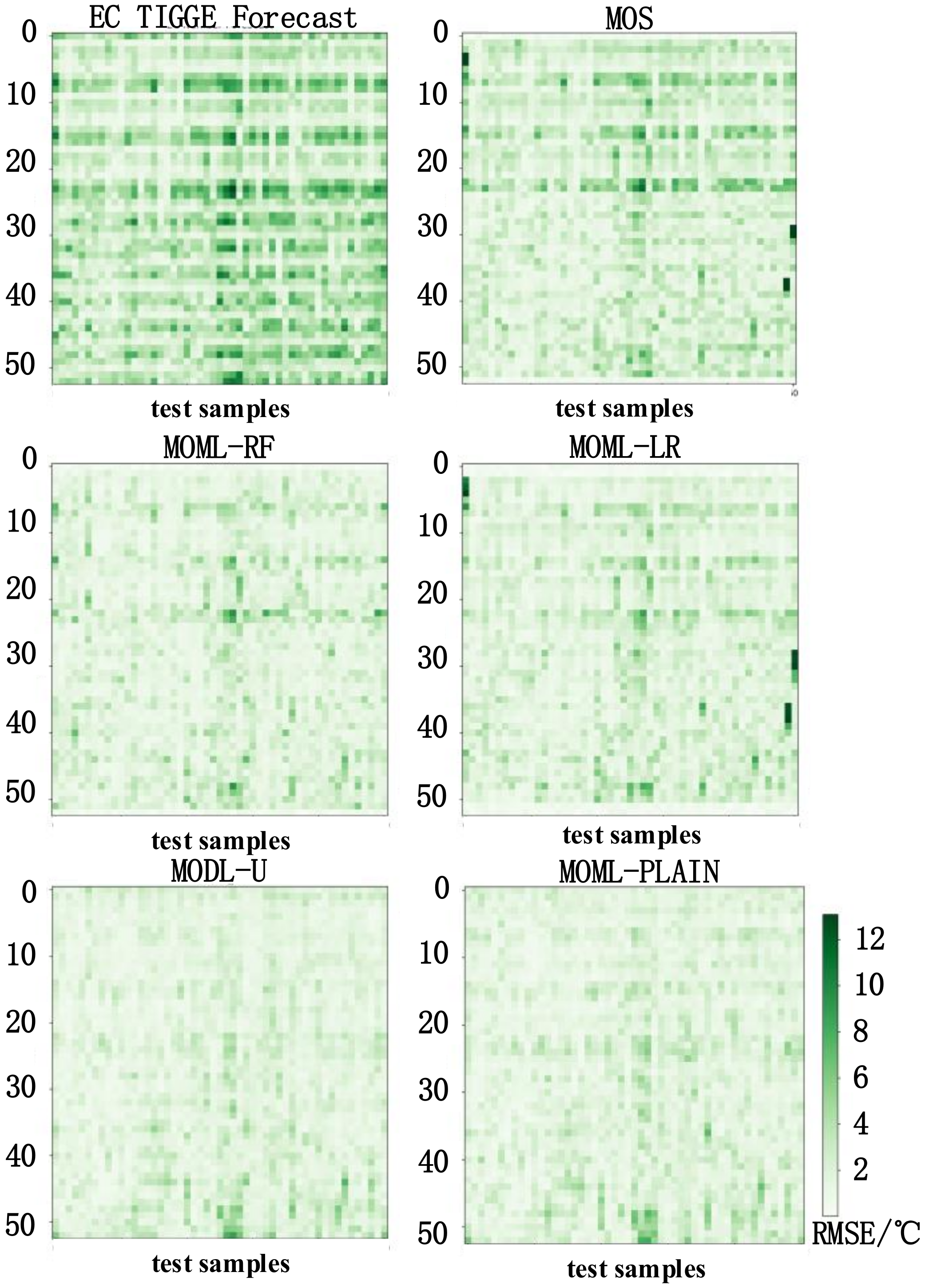
The forecast deviation of models in the test dataset is expanded into a deviation comparison matrix in both dimensions of the date and the forecast time which is plotted in the form of a heat map in Figure 12 to compare the post-processing effects of different models for different dates and different time steps. For an element of the contrast matrix with the coordinates , the shade of its grid color means the of the forecast step on the test date . The darker the element is, the greater the error is, and the worse the prediction effect is. On the contrary, the lighter the part is, the prediction result is closer to the observation result.
According to Figure 12, the better the EC data, the better the forecast results. It means that the improved models can only post-process based on the deviation of the learned observation data from the EC data. The seasonal impact of EC temperature forecast results is not enormous. Accordingly, the seasonality of the post-processing algorithm is not obvious. Of the six error heat maps, the two heat maps for MODL forecasts have the lightest color, which shows that the MODL forecast has the best effect.
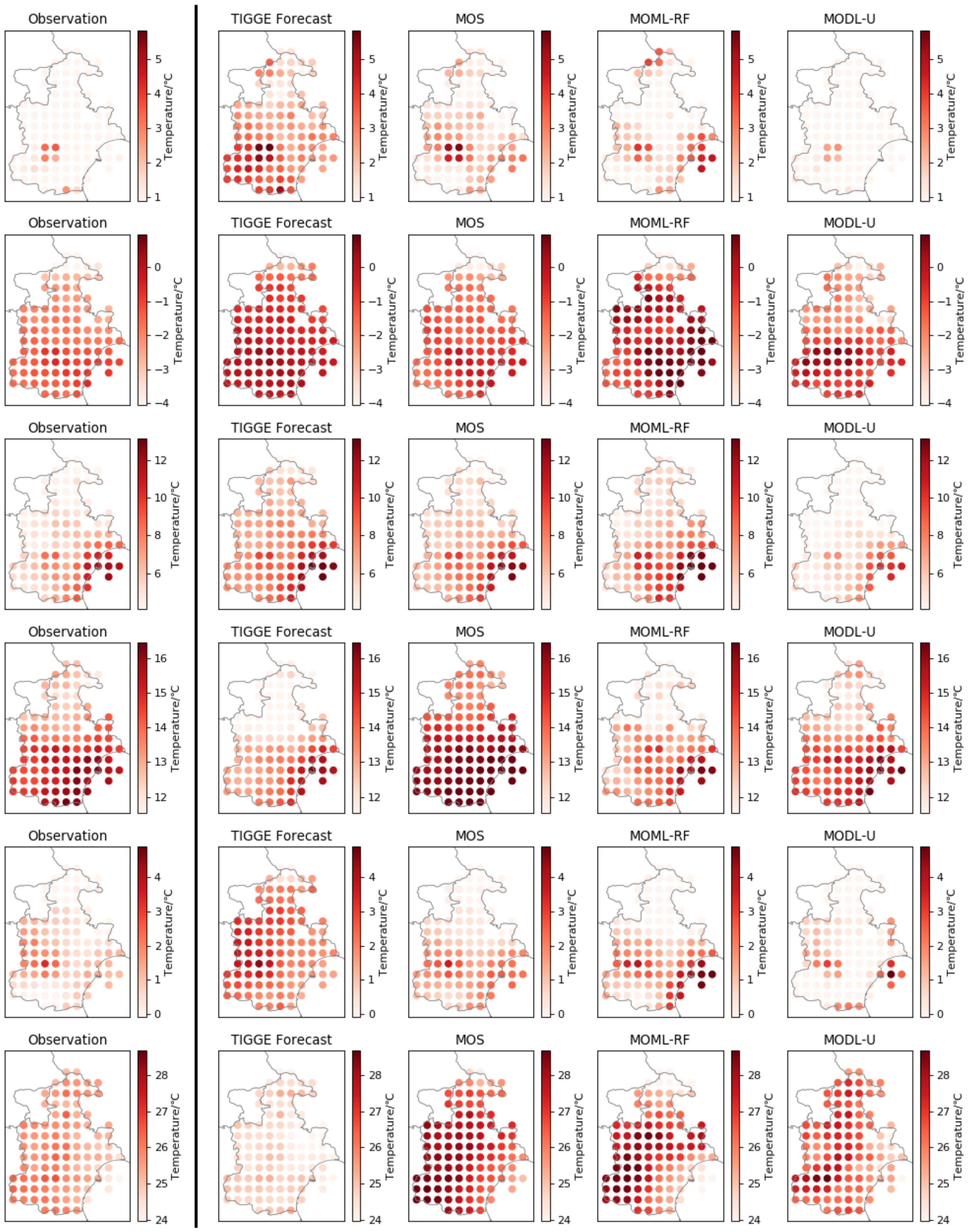
Finally, the experiment randomly selected the forecast data at six forecast moments from test dataset for visualization in Figure 13 in order to show the improvement effect of MODL more clearly. Because of space limitations, in addition to the observed temperature field, TIGGE forecast temperature field, and MOS forecast temperature field, we have selected the MOML-RF and MODL-U forecasted temperature fields that perform better in MOML and MODL to visualize them. Through horizontal comparison, it can be seen that most of the MODL-U forecast temperature field is closer to the observed temperature field. This shows that the post-processing effect of MODL-U is better. However, there is also a situation like the last line, the forecasting effect of different post-processing algorithms is not as good as the EC forecasting effect. This may be related to other weather elements being used in the post-processing model modeling. In addition, it should be noted that, in the same subgraph, some grid points are closer to the real temperature after post-processing, while some grid points have worse prediction effect after post-processing. This is related to the geographical location of the grid and the density of observation stations around the grid. Intuitively, the post-processing effect of MODL-U is better than other post-processing algorithms.
4.3. Comparison of MODL-PLAIN and MODL-U
This subsection will compare MODL-U and MODL-PLAIN. The various statistical performance of MODL-U is better than MODL-PLAIN due to the integration of the features of different time and space scales. MODL-U has a smaller and a larger in Table 3. The error of MODL-U at different forecast lead times are also smaller than MODL-PLAIN, which can be seen in Figure 10. The smaller rectangular area of MODL-U in Figure 11 shows its higher robustness. The shallower comparison matrix in Figure 12 shows that MODL-U is better than MODL-PLAIN for any forecast lead time and any forecast date. It can be seen that the multi-scale MODL model has better forecasting capabilities.
However, for deep learning models, the demand for computing resources is also an important measurement. This directly affects whether the MODL algorithm can be applied to the weather consultation of the meteorological department. The indexes that affect the application ability of model engineering include model size, memory requirements, floating point operations (FLOPs), and parameter-number. Models with large storage space and high memory requirements cannot be run on computers with low configuration. Models with massive FLOPs require more computing power. Table 4 compares the above indicators of MODL-U and MODL-PLAIN.
The storage space is the space occupied by the trained model on the hard disk. MODL-PLAIN and MODL-U take up little storage space and have low demand for the machine. The memory requirements in the table are the memory required for testing when batch size = 128. When the computer uses the MODL model for post-processing, it will read the model parameters from the hard disk to the internal memory. In addition, the matrix calculation also requires memory when the model is running. Too many requests for memory will slow down the speed of the computer. MODL-U requires a computer with at least 8 GB memory and MOML-PLAIN only needs 4 GB. FLOPs is a measure of computer performance, useful in fields of scientific computations that require floating-point calculations. FLOPs can reflect the speed of the calculation. MODL-U has twice as much floating-point calculation as MODL-PLAIN. The parameter-number is the total amount of and in the formula (4). MODL-PLAIN has less than half of MODL-U’s parameter-numbers. During post-processing, MODL-PLAIN will run much faster than MODL-U, because of the parameter-number and FLOPs. Therefore, MODL-PLAIN is a lightweight model. In actual operations, if better forecast results are needed, the MODL-U model can be used for the post-processing of NWP. MODL-PLAIN can be used as an alternative model when the computer configuration is not sufficient to run MODL-U, or the processing results need to be obtained quickly.
5. Conclusions
This paper proposes a temperature forecast model that is based on deep learning methods, called MODL. The novelty of MODL focuses on the application of advanced deep learning modules to improve the prediction accuracy of the global numerical model ECMWF. The principal work of this paper is the design and application of MODL model. Two MODL models with base skeleton structure are proposed, namely MODL-PLAIN and MODL-U. The MODL can deliver outputs (in the form of more accurate ECMWF prediction) in real-time, and it is easy to use by both professionals and basic end-users. Although the forecasting effect of MODL is affected by the input (ECMWF forecast data), the improvement effect of the MODL model on different dates and at different times is obvious.
In summary, the MODL method is better than the univariate linear MOS method, the MOML method based random forest, and linear regression with a running period, and it has the ability to improve grid temperature forecast results in Tianjin area. Besides, MODL can be implemented in the weather consultation process as a post-processing method with high-grade application prospects and it can significantly reduce human resources expenditure in the weather consultation process. In terms of its practical applicability, it is not necessary to retrain the model when using the deep learning algorithm that is mentioned in this article to process data within two years. The prediction results can be quickly obtained. Our future research direction is to explore the application of different deep learning modules in the interpretability of weather forecast and the generalization ability of the model in different regions with different weather elements. In addition, finding the weather elements related to the 2 m air temperature and evaluating the model that is based on the sub-sampling results of these elements is also worthy of further study.
Author Contributions
Conceptualization, D.W.; Data curation, X.Y. and N.Z.; Formal analysis, N.Z. and D.W.; Funding acquisition, X.Y.; Investigation, K.C., P.W. and D.W.; Methodology, D.W.; Project administration, D.W.; Resources, P.W. and D.W.; Software, K.C.; Supervision, P.W.; Validation, X.Y. and N.Z.; Visualization, K.C.; Writing—original draft, K.C.; Writing—review & editing, D.W. All authors have read and agreed to the published version of the manuscript.
Funding
This work was supported by the National Natural Science Foundation of China under Grant 61972282.
Conflicts of Interest
The authors declare no conflict of interest.
References
- Zhang, C.; Zeng, J.; Wang, H.; Ma, L.; Chu, H. Correction model for rainfall forecasts using the LSTM with multiple meteorological factors. Meteorol. Appl. 2019, 27, e1852. [Google Scholar] [CrossRef] [Green Version]
- Kalnay, E.; Kanamitsu, M.; Kistler, R.; Collins, W.; Deaven, D.; Gandin, L.; Iredell, M.; Saha, S.; White, G.; Woollen, J.; et al. The NCEP/NCAR 40-Year Reanalysis Project. Bull. Amer. Meteor. Soc. 1996, 77, 437–472. [Google Scholar] [CrossRef] [Green Version]
- Huffman, G.J.; Adler, R.F.; Rudolf, B.; Schneider, U.; Keehn, P.R. Global Precipitation Estimates Based on a Technique for Combining Satellite-Based Estimates, Rain Gauge Analysis, and NWP Model Precipitation Information. J. Clim. 1995, 8, 1284–1295. [Google Scholar] [CrossRef] [Green Version]
- Molteni, F.; Buizza, R.; Palmer, T.N.; Petroliagis, T. The ECMWF ensemble prediction system: Methodology and validation. Q. J. R. Meteorol. Soc. 1996, 122, 73–119. [Google Scholar] [CrossRef]
- Toth, Z.; Kalnay, E. Ensemble Forecasting at NCEP and the Breeding Method. Mon. Weather. Rev. 1997, 125, 3297–3319. [Google Scholar] [CrossRef]
- García-Pereda, J.; Fernández-Serdán, J.M.; Alonso, Ó.; Sanz, A.; Guerra, R.; Ariza, C.; Santos, I.; Fernández, L. NWCSAF High Resolution Winds (NWC/GEO-HRW) Stand-Alone Software for Calculation of Atmospheric Motion Vectors and Trajectories. Remote. Sens. 2019, 11, 2032. [Google Scholar] [CrossRef] [Green Version]
- Miyoshi, T.; Otsuka, S.; Honda, T.; Lien, G.Y.; Maejima, Y.; Yoshizaki, Y.; Seko, H.; Tomita, H.; Satoh, S.; Ushio, T.; et al. Big Data Assimilation: Past 5 Years and Perspectives for the Future. Geophys. Res. Abstr. 2019, 21, 1. [Google Scholar]
- Mujeeb, S.; Alghamdi, T.; Ullah, S.; Fatima, A.; Javaid, N.; Saba, T. Exploiting Deep Learning for Wind Power Forecasting Based on Big Data Analytics. Appl. Sci. 2019, 9, 4417. [Google Scholar] [CrossRef] [Green Version]
- Privé, N.C.; Errico, R.M. The role of model and initial condition error in numerical weather forecasting investigated with an observing system simulation experiment. Tellus Dyn. Meteorol. Oceanogr. 2013, 65, 21740. [Google Scholar] [CrossRef]
- Bao, X.W.; Ma, L.M. Research Progress on Physical Parameterization Schemes in Numerical Weather Prediction Models. Adv. Earth Sci. 2017, 32, 679–687. [Google Scholar]
- Mu, M.; Chen, B.Y.; Zhou, F.F.; Yu, Y.S. Methods and Uncertainty of Weather Forecast. Meteorological 2011, 37, 1–13. [Google Scholar]
- Qiao, S.; Zou, M.; Cheung, H.N.; Zhou, W.; Li, Q.; Feng, G.; Dong, W. Predictability of the wintertime 500 hPa geopotential height over Ural-Siberia in the NCEP climate forecast system. Clim. Dyn. 2019, 54, 1591–1606. [Google Scholar] [CrossRef]
- Palmer, T. The ECMWF ensemble prediction system: Looking back (more than) 25 years and projecting forward 25 years. Q. J. R. Meteorol. Soc. 2018, 145, 12–24. [Google Scholar] [CrossRef] [Green Version]
- Xia, J.; Li, H.; Kang, Y.; Yu, C.; Ji, L.; Wu, L.; Lou, X.; Zhu, G.; Wang, Z.; Yan, Z.; et al. Machine Learning-based Weather Support for the 2022 Winter Olympics. Adv. Atmos. Sci. 2020, 37, 927–932. [Google Scholar] [CrossRef]
- Gao, M.; Li, J.; Hong, F.; Long, D. Long Short-Term Forecasting of Power Production in a Large-Scale Photovoltaic Plant Based on LSTM. Appl. Sci. 2019, 9, 3192. [Google Scholar] [CrossRef] [Green Version]
- Shan, Y.; Zhang, R.; Gultepe, I.; Zhang, Y.; Gultepe, I.; Wang, Y. Gridded Visibility Products over Marine Environments Based on Artificial Neural Network Analysis. Appl. Sci. 2019, 9, 4487. [Google Scholar] [CrossRef] [Green Version]
- Lian, J.; Dong, P.; Zhang, Y.; Pan, J. A Novel Deep Learning Approach for Tropical Cyclone Track Prediction Based on Auto-Encoder and Gated Recurrent Unit Networks. Appl. Sci. 2020, 10, 3965. [Google Scholar] [CrossRef]
- Glahn, H.R.; Lowry, D.A. The use of model output statistics (MOS) in objective weather forecasting. J. Appl. Meteorol. 1972, 11, 1203–1211. [Google Scholar] [CrossRef] [Green Version]
- Peng, X.; Che, Y.; Chang, J. A novel approach to improve numerical weather prediction skills by using anomaly integration and historical data. J. Geophys. Res. Atmos. 2013, 118, 8814–8826. [Google Scholar] [CrossRef]
- Sloughter, J.M.; Gneiting, T.; Raftery, A.E. Probabilistic Wind Speed Forecasting Using Ensembles and Bayesian Model Averaging. J. Am. Stat. Assoc. 2010, 105, 25–35. [Google Scholar] [CrossRef] [Green Version]
- Yang, D. On post-processing day-ahead NWP forecasts using Kalman filtering. Sol. Energy 2019, 182, 179–181. [Google Scholar] [CrossRef]
- Nerini, D.; Foresti, L.; Leuenberger, D.; Robert, S.; Germann, U. A Reduced-Space Ensemble Kalman Filter Approach for Flow-Dependent Integration of Radar Extrapolation Nowcasts and NWP Precipitation Ensembles. Mon. Weather. Rev. 2019, 147, 987–1006. [Google Scholar] [CrossRef]
- Li, H.; Yu, C.; Xia, J.; Wang, Y.; Zhu, J.; Zhang, P. A Model Output Machine Learning Method for Grid Temperature Forecasts in the Beijing Area. Adv. Atmos. Sci. 2019, 36, 1156–1170. [Google Scholar] [CrossRef]
- Zheng, A.; Casari, A. Feature Engineering for Machine Learning: Principles and Techniques for Data Scientists; O’Reilly Media Inc.: Sebastopol, CA, USA, 2018. [Google Scholar]
- Koza, J.R.; Bennett, F.H.; Andre, D.; Keane, M.A. Automated Design of Both the Topology and Sizing of Analog Electrical Circuits Using Genetic Programming. In Artificial Intelligence in Design’96; Gero, J.S., Sudweeks, F., Eds.; Springer: Berlin/Heidelberg, Germany, 1996; pp. 151–170. [Google Scholar]
- Ardabili, S.; Mosavi, A.; Dehghani, M.; Várkonyi-Kóczy, A.R. Deep Learning and Machine Learning in Hydrological Processes Climate Change and Earth Systems a Systematic Review. In Proceedings of the Engineering for Sustainable Future, PyeongChang, Korea, 16–19 February 2020; Várkonyi-Kóczy, A.R., Ed.; Springer International Publishing: Cham, Switzerland, 2020; pp. 52–62. [Google Scholar]
- Voulodimos, A.; Doulamis, N.; Doulamis, A.; Protopapadakis, E. Deep Learning for Computer Vision: A Brief Review. Comput. Intell. Neurosci. 2018, 2018, 1–13. [Google Scholar] [CrossRef]
- Nassif, A.B.; Shahin, I.; Attili, I.; Azzeh, M.; Shaalan, K. Speech Recognition Using Deep Neural Networks: A Systematic Review. IEEE Access 2019, 7, 19143–19165. [Google Scholar] [CrossRef]
- Sorin, V.; Barash, Y.; Konen, E.; Klang, E. Deep Learning for Natural Language Processing in Radiology—Fundamentals and a Systematic Review. J. Am. Coll. Radiol. 2020, 17, 639–648. [Google Scholar] [CrossRef]
- Zambrano, F.; Vrieling, A.; Nelson, A.; Meroni, M.; Tadesse, T. Prediction of drought-induced reduction of agricultural productivity in Chile from MODIS, rainfall estimates, and climate oscillation indices. Remote Sens. Environ. 2018, 219, 15–30. [Google Scholar] [CrossRef]
- Hossain, M.; Rekabdar, B.; Louis, S.J.; Dascalu, S. Forecasting the weather of Nevada: A deep learning approach. In Proceedings of the International Joint Conference on Neural Networks (IJCNN), Killarney, Ireland, 12–16 July 2015; pp. 1–6. [Google Scholar]
- Dupuy, F.; Mestre, O.; Serrurier, M.; Bakkay, M.C.; Burdá, V.C.; Cabrera-Gutiérrez, N.C.; Jouhaud, J.C.; Mader, M.A.; Oller, G.; Zamo, M. ARPEGE cloud cover forecast post-processing with convolutional neural network. arXiv 2020, arXiv:2006.1667. [Google Scholar]
- Wang, K.; Qi, X.; Liu, H.; Song, J. Deep belief network based k-means cluster approach for short-term wind power forecasting. Energy 2018, 165, 840–852. [Google Scholar] [CrossRef]
- Long, J.; Shelhamer, E.; Darrell, T. Fully Convolutional Networks for Semantic Segmentation. In Proceedings of the IEEE Conference on Computer Vision and Pattern Recognition, Boston, MA, USA, 7–12 June 2015. [Google Scholar]
- Li, B. 3D Fully Convolutional Network for vehicle detection in point cloud. In Proceedings of the IEEE/RSJ International Conference on Intelligent Robots and Systems, Vancouver, BC, Canada, 24–28 September 2017. [Google Scholar]
- Janssens, R.; Zeng, G.; Zheng, G. Fully automatic segmentation of lumbar vertebrae from CT images using cascaded 3D Fully Convolutional Networks. In Proceedings of the IEEE 15th International Symposium on Biomedical Imaging, Washington, DC, USA, 4–7 April 2018. [Google Scholar]
- Ronneberger, O.; Fischer, P.; Brox, T. U-Net: Convolutional Networks for Biomedical Image Segmentation. In Proceedings of the Medical Image Computing and Computer-Assisted Intervention, Munich, Germany, 5–9 October 2015. [Google Scholar]
- Gultepe, I.; Sharman, R.; Williams, P.D.; Zhou, B.; Ellrod, G.; Minnis, P.; Trier, S.; Griffin, S.; Yum, S.S.; Gharabaghi, B.; et al. A Review of High Impact Weather for Aviation Meteorology. Pure Appl. Geophys. 2019, 176, 1869–1921. [Google Scholar] [CrossRef]
- Cressman, G.P. An operational objective analysis system. Mon. Weather Rev. 1959, 87, 367–374. [Google Scholar] [CrossRef]
- Gu, J.; Wang, Y.; Xie, D.; Zhang, Y. Wind Farm NWP Data Preprocessing Method Based on t-SNE. Energies 2019, 12, 3622. [Google Scholar] [CrossRef] [Green Version]
- Lian, J.; Dong, P.; Zhang, Y.; Pan, J.; Liu, K. A Novel Data-Driven Tropical Cyclone Track Prediction Model Based on CNN and GRU with Multi-Dimensional Feature Selection. IEEE Access 2020, 8, 97114–97128. [Google Scholar] [CrossRef]
- Li, Q.; Yue, S.; Wang, Y.; Ding, M.; Li, J.; Wang, Z. Boundary Matching and Interior Connectivity-Based Cluster Validity Anlysis. Appl. Sci. 2020, 10, 1337. [Google Scholar] [CrossRef] [Green Version]
- Pal, M. Random forest classifier for remote sensing classification. Int. J. Remote. Sens. 2005, 26, 217–222. [Google Scholar] [CrossRef]
- Krizhevsky, A.; Sutskever, I.; Hinton, G.E. ImageNet Classification with Deep Convolutional Neural Networks. In Proceedings of the Advances in Neural Information Processing Systems 25, Granada, Spain, 12–14 December 2011. [Google Scholar]
- Szegedy, C.; Liu, W.; Jia, Y.; Sermanet, P.; Reed, S.; Anguelov, D.; Erhan, D.; Vanhoucke, V.; Rabinovich, A. Going Deeper with Convolutions. In Proceedings of the IEEE Conference on Computer Vision and Pattern Recognition, Boston, MA, USA, 7–12 June 2015. [Google Scholar]
- Klambauer, G.; Unterthiner, T.; Mayr, A.; Hochreiter, S. Self-Normalizing Neural Networks. In Proceedings of the Advances in Neural Information Processing Systems 30, Long Beach, CA, USA, 4–9 December 2017. [Google Scholar]
- Glorot, X.; Bordes, A.; Bengio, Y. Deep sparse rectifier neural networks. In Proceedings of the Fourteenth International Conference on Artificial Intelligence and Statistics, Fort Lauderdale, FL, USA, 11–13 April 2011. [Google Scholar]
- Santurkar, S.; Tsipras, D.; Ilyas, A.; Mądry, A. How does batch normalization help optimization? Adv. Neural Inf. Process. Syst. 2018, 2018, 2483–2493. [Google Scholar]
Figure 1.
Visualization of model forecast data. Each two-dimensional (2D) heat map represents the distribution of a single weather element at a single time. For each weather element, all of the corresponding heat maps in the first column are concatenated through time to form the three-dimensional (3D) tensor in the second column. Different color tensors represent different weather elements. Twenty-one 3D tensors correspond to 21 types of weather elements. The 3D tensors are concatenated to obtain the four-dimensional (4D) tensor on the right side of Figure 1. Each four-dimensional tensor is a sample in the experiment.

Figure 2.
Visualization of observational data. The first column in the figure is the site observation data at 53 time steps. The second column is the grid observation data after inverse distance interpolation. The third column is the 3D tensor obtained by concatenating the tensor in the second column in the time dimension.

Figure 3.
The training and operational process of model output deep learning (MODL).

Figure 4.
The base framework of MODL.

Figure 5.
3D Fully Convolutional Neural Network Model (MODL-PLAIN) structure. The seven-channel tensor on the left is the input of the model, which is the seven weather elements of the numerical forecast model. The single-channel tensor on the right is the output of the model, which is the forecast result of MODL-PLAIN. The three green tensors in the middle are the output feature tensors of the middle convolutional layer. The feature tensor has the same shape and different channels.

Figure 6.
MODL-PLAIN spatial information integration scope. Different administrative areas in each map are painted in different colors according to the observed temperature.
Figure 6.
MODL-PLAIN spatial information integration scope. Different administrative areas in each map are painted in different colors according to the observed temperature.

Figure 7.
Three-Dimensional (3D) Fully Convolutional Neural Network based on U-Net Structure. The 7-channel tensor on the left is the input of the model, which is the seven weather elements of the numerical forecast model. The single-channel tensor on the right is the output of the model, which is the forecast result of MODL-PLAIN. The three green tensors in the middle are the output feature tensors of the middle convolutional layer. The feature tensor of the same row has the same shape and the number of channels is different. Max pool is the downsampling layer, Up conv is the upsampling layer, and the concatenate operation performs tensor splicing in the channel dimension.

Figure 8.
Variable metric in time scale processing.

Figure 9.
Eight-fold cross-validation of experimental data. Training is the process of training the model using the selected hyperparameter in the training set. Evaluating is the process of saving the optimal model based on the validation set’s score. Testing is the process of evaluating the hyperparameters by calculating each folding model’s scores on the test set.

Figure 10.
Forecast error’s daily root-mean-square error (RMSE).

Figure 11.
Error box plot. Each box plot corresponds to the distribution of a model forecast error. The ordinate of the green line in the box is the median of the error distribution, and the ordinate of the green triangle is the mean of the error distribution. The upper and lower sides of the box are the upper quartiles (Q3) and lower quartiles (Q1) of the error distribution. The two horizontal lines on the outside of the box are the maximum and minimum values of non-abnormal error data. Each circle represents an abnormal error.

Figure 12.
Comparison matrix of RMSE for different post-processing methods. The total number of samples in the test set is 1032 × 0.2 ≈ 206, including 51 dates in 12 months throughout 2017. A forecast will be made for a test date. Each time it will forecast the temperature at 53 steps in the future. Therefore, the horizontal axis of the heat map is 51 test times arranged in date order in 2017. The vertical axis is the 53 steps forecast for each forecast date. The pixel value of the heat map indicates the error between the forecast temperature and the observed temperature. The deviation evaluation index is the root mean square error (RMSE).

Figure 13.
2 m air temperature forecast visualization comparison figure. The figure visualizes the observation results of 2 m temperature and the forecast results of different forecast models at six different time steps. Each row of pictures corresponds to a temperature field at a time step. From left to right is the observation field, TIGGE forecast field, MOS forecast field, MOML-RF forecast field and MODL-U forecast field. Each dot on the subgraph represents the temperature of a valid forecast grid point. The shade of the color indicates the level of temperature.


Table 1.
Parameter combination range.
| Parameters Abbreviation | Range |
|---|---|
| n_estimators | (50,120,160,200,250) |
| max_depth | (1,2,3,5,7,9,11,13) |
| min_samples_leaf | (1,5,10,20,30,40) |
| max_features | (3,5,7,9) |
Table 2.
Weather elements, abbreviations, and correlations.
| Predictor | Abbreviation | Level | Score (%) |
|---|---|---|---|
| 10-m U wind component | 10u | - | 9.249 |
| 10-m V wind component | 10v | - | 10.006 |
| 2 m dewpoint temperature | 2d | - | 4.893 |
| 2 m temperature | 2t | - | - |
| Convective available potential energy | cape | - | 0.126 |
| Low cloud cover | lcc | - | 0.032 |
| Mean sea level pressure | msl | - | 9.091 |
| Relative humidity | r | 850 hPa | 4.766 |
| Relative humidity | r | 925 hPa | 3.946 |
| Relative humidity | r | 950 hPa | 4.104 |
| Temperature | T | 850 hPa | 7.481 |
| Temperature | T | 925 hPa | 14.426 |
| Total cloud cover | tcc | - | 3.030 |
| Total precipitation | tp | - | 2.052 |
| Visibility | vis | - | 7.797 |
| U wind component | u | 850 hPa | 1.042 |
| U wind component | u | 925 hPa | 4.766 |
| U wind component | u | 950 hPa | 4.893 |
| V wind component | v | 850 hPa | 2.241 |
| V wind component | v | 925 hPa | 2.620 |
| V wind component | v | 950 hPa | 3.441 |
Table 3.
Model performance on the test set.
| Methods | EC | MOS | MOML-LR | MOML-RF | MODL-U | MODL-PLAIN |
|---|---|---|---|---|---|---|
| RMSE | 4.0667 | 3.0154 | 2.5388 | 2.2206 | 1.9542 | 2.0147 |
| Acc | 69.5 | 70.21 | 74.53 | 77.71 | 80.65 | 79.51 |
Table 4.
Comparison of evaluation indexes of different models.
| MODL-PLAIN | MODL-U | |
|---|---|---|
| storage space | 172 KB | 690 KB |
| memory requirements | 3.9 GB | 6.5 GB |
| FLOPs | 0.558 GB | 1.354 GB |
| parameter-number | 0.041 MB | 0.1 MB |
© 2020 by the authors. Licensee MDPI, Basel, Switzerland. This article is an open access article distributed under the terms and conditions of the Creative Commons Attribution (CC BY) license (http://creativecommons.org/licenses/by/4.0/).
Share and Cite
MDPI and ACS Style
Chen, K.; Wang, P.; Yang, X.; Zhang, N.; Wang, D. A Model Output Deep Learning Method for Grid Temperature Forecasts in Tianjin Area. Appl. Sci. 2020, 10, 5808. https://doi.org/10.3390/app10175808
AMA Style
Chen K, Wang P, Yang X, Zhang N, Wang D. A Model Output Deep Learning Method for Grid Temperature Forecasts in Tianjin Area. Applied Sciences. 2020; 10(17):5808. https://doi.org/10.3390/app10175808
Chicago/Turabian StyleChen, Keran, Ping Wang, Xiaojun Yang, Nan Zhang, and Di Wang. 2020. "A Model Output Deep Learning Method for Grid Temperature Forecasts in Tianjin Area" Applied Sciences 10, no. 17: 5808. https://doi.org/10.3390/app10175808
Note that from the first issue of 2016, this journal uses article numbers instead of page numbers. See further details here.