Hybrid Learning of Hand-Crafted and Deep-Activated Features Using Particle Swarm Optimization and Optimized Support Vector Machine for Tuberculosis Screening

Abstract

Tuberculosis (TB) is a leading infectious killer, especially for people with Human Immunodeficiency Virus (HIV) and Acquired Immunodeficiency Syndrome (AIDS). Early diagnosis of TB is crucial for disease treatment and control. Radiology is a fundamental diagnostic tool used to screen or triage TB. Automated chest x-rays analysis can facilitate and expedite TB screening with fast and accurate reports of radiological findings and can rapidly screen large populations and alleviate a shortage of skilled experts in remote areas. We describe a hybrid feature-learning algorithm for automatic screening of TB in chest x-rays: it first segmented the lung regions using the DeepLabv3+ model. Then, six sets of hand-crafted features from statistical textures, local binary pattern, GIST, histogram of oriented gradients (HOG), pyramid histogram of oriented gradients and bags of visual words (BoVW), and nine sets of deep-activated features from AlexNet, GoogLeNet, InceptionV3, XceptionNet, ResNet-50, SqueezeNet, ShuffleNet, MobileNet, and DenseNet, were extracted. The dominant features of each feature set were selected using particle swarm optimization, and then separately input to an optimized support vector machine classifier to label ‘normal’ and ‘TB’ x-rays. GIST, HOG, BoVW from hand-crafted features, and MobileNet and DenseNet from deep-activated features performed better than the others. Finally, we combined these five best-performing feature sets to build a hybrid-learning algorithm. Using the Montgomery County (MC) and Shenzen datasets, we found that the hybrid features of GIST, HOG, BoVW, MobileNet and DenseNet, performed best, achieving an accuracy of 92.5% for the MC dataset and 95.5% for the Shenzen dataset.

1. Introduction

Infectious diseases are threats to global health: one is tuberculosis (TB), a serious contagious disease that can be easily transmitted. TB is spread through the air when a TB infected person coughs, sneezes or spits. It is caused by the Mycobacterium tuberculosis. The World Health Organization (WHO) estimated that around 11 million people were ill with TB in 2019 worldwide and 1.5 million died. The early and accurate detection of TB is essential to control the disease progression and to prevent forward transmissions. The WHO recommends that a chest x-ray is an essential tool to end TB. Chest x-rays are non-invasive, fast, affordable, highly sensitive and widely available in urban areas. Chest x-rays are used to screen or triage TB in the lungs and to follow up the treatment. TB mostly affects the lungs and when TB lesions appear in the lungs, the chest x-rays will display abnormal grey or white shadows [1,2].

Conventional examination of chest x-rays needs a high degree of expertise, takes time and is prone to human errors. With the advent of digital imaging and advanced computer vision methods, computer-assisted diagnosis (CAD) of the diseases, computational techniques have been evaluated in several types of research. CAD systems aim to assist the medical experts in identifying the disease and to serve as a complement to human reading of medical images. With the support of CAD systems, we can detect TB accurately and rapidly, and possibly prevent further transmissions, if it is detected early. CAD systems have the potential to expedite mass screening programs in high TB prevalence areas, where a large number of x-rays need to be examined. They can also alleviate the shortage of qualified medical staff, especially in remote areas [3].

Previous studies of automatic TB prediction in chest x-rays may be categorized into two groups: (i) hand-crafted feature-based machine learning methods and (ii) deep convolutional neural network (CNN) based methods. Both categories work with or without lung segmentation. For the first category, Ginneken et al. [4] used multi-scale feature banks as the inputs to a weighted nearest-neighbor classifier to identify the presence of TB and obtained area under curve (AUC) of 98.6% and 82% on two private datasets. An algorithm by Hogeweg et al. [5] analyzed texture abnormality at the pixel level and provided AUCs between 67% and 86%. Tan et al. [6] used a user-guided snake algorithm for lung segmentation, and first-order statistical features as features to be classified by a decision tree classifier for TB prediction. On a small custom dataset, their accuracy was 94.9%. Jaeger et al. [7] used optimized graph cut methods for lung segmentation and object detection inspired features and content retrieval ones as input to a support vector machine (SVM) classifier. They obtained AUCs of 86.9% for the Montgomery County (MC) dataset and 90% for Shenzen datasets. Vajda et al. [8] segmented the lung using an atlas-driven method and extracted multi-level features of shape, curvature and Hessian matrix eigenvalues. Following this, the wrapper type feature selection with a multi-layer perceptron was used to select the discriminant features and differentiate between normal and TB chest x-rays: they achieved AUCs of 87% for MC and 99% for Shenzen. Karargyris et al. [9] segmented the lung region using an atlas-driven method, extracted a combined feature set of texture and shape, and applied SVM as a classifier and obtained AUC of 93.4% for the Shenzen dataset. Jemal [10] used another texture feature-based method, after segmenting the lung region by thresholding; he extracted the textural features, and then differentiated between positive and negative using SVM, achieving AUCs of 71% for MC and 91% for Shenzen. Santosh and Antani [11] used multi-scale features of shape, edge, and texture, and a combination of a Bayes network, Multilayer Perceptron (MLP) and a random forest, yielding AUCs of 90% for MC and 96% for Shenzen dataset. Multiple instance learning methods [12] used moments of pixel intensities as features and SVM as a classifier and led to AUCs between 86% and 91% for three private datasets. Besides, the prediction scores were used to indicate the diseased regions using heat maps. Melendez et al. used the combined feature set of local/global features from chest x-rays and clinical information and selected the optimal feature subset using the minimum redundancy maximum relevant (mRMR) method [13]. Using the selected features, an ensemble classifier of random forest and extremely randomized trees was used to predict TB: they obtained AUCs of 99.6% for MC and 97.7 for Shenzen datasets. Chauhan et al. [14] used GIST and pyramid histogram of oriented gradients (PHOG), as the feature extractors, and SVM, as the classifier, and tested two custom datasets: Dataset A and DataSet B. They achieved promising results using PHOG features with an accuracy of 92.3% for Dataset A and 92.0% for Dataset B. These studies and their results show that the handcrafted features are suitable for classifying normal and TB containing x-rays.

In recent years, deep CNNs have achieved human experts-level performance on automated detection of diseases on a diversity of medical images. For example, Esteva et al. [15] achieved dermatologist-level performance on skin cancer detection and Rajpurkar et al. [16] outperformed the conventional methods and achieved the radiologist-level pneumonia detection. We found four different strategies using CNNs to detect diseases in medical images: training the new CNN architecture from scratch, fine-tuning of pre-trained CNNs, use of pre-trained CNNs as the feature descriptors and the integration of deep features from pre-trained CNNs with shallow hand-crafted features. Pasa et al. described a modified CNN model, a variant of AlexNet, with a depth of five convolutional blocks and additional skip connections [17]; they achieved AUCs of 81.1% for MC and 90% for Shenzen datasets and used their model to generate the saliency maps and gradient-weighted class activation mapping (Grad-CAM) to localize the disease regions. Despite the promising results, training the model from scratch presents significant challenges, because it demands the high computational resources and a large volume of data. Training the model from scratch using a small dataset may over-fit. When there is only a small dataset available, fine-tuning of the pre-trained CNNs on certain images is an alternative to training the network from scratch, while achieving similar results. For example, Hwang et al. [18] adopted the transfer learning using the pre-trained AlexNet and achieved AUCs of 88.4% for MC and 92.6% for Shenzen datasets. Islam et al. [19] used Alexnet, VGG16, VGG19, ResNet-18, ResNet-50, and ResNet-152 CNN models separately and combined their results to make a final prediction decision, using the Shenzen dataset, they found an AUC of 94%. Similarly, Lakhani and Sundaram [20] used an ensemble learner, combining the output of AlexNet and GoogLeNet, and evaluated it on four different datasets with 1007 images, they achieved AUC of 99%. Even fine-tuning the pre-trained models, it took time to train and parameters to tune. Therefore, Lopes et al. [21] and Rajaraman et al. [22] showed how to use pre-trained CNNs as the feature extractors, this technique is called deep-activated features or deep features. Lopes et al. [21] used the pre-trained CNNs as the features descriptors. Deep activated features from GoogleNet, ResNet, and VGGNet were extracted in three different approaches and fed separately as input to the SVM classifier. They obtained the highest AUC of 92.6% for MC and Shenzen datasets. Rajaraman et al. [22] first segmented the lung region, using an atlas-based method, and built the SVM classifiers using hand-crafted features, and deep-activated features from pre-trained CNN models, separately. Finally, they built an ensemble-stacked model of different based learners via majority voting. Using four datasets, they reported AUCs of 98.6% for MC, 99.4% for Shenzen, plus two additional datasets that they built—Kenya 82.9% and India 99.5%. The fourth strategy of using pre-trained CNNs, which is the focus of our work, was a combination of deep-activated features, extracted from pre-trained CNNs, with hand-crafted features, to design a more efficient and accurate classifier. Extracting multiple deep features from pre-trained CNNs and integrating them with shallow handcrafted features is a promising way to further enhance the performance, compared to using an individual feature set.

Most of the hand-crafted and deep-activated features in this study have been used in TB detection. However, except the studies in Vajda et al. [8] and Melendez et al. [13], all extracted features were used as input to the classification, so the feature set might contain noise and irrelevant features. To address this lack, we used a particle swarm optimization (PSO) algorithm to select the discriminant features before classification. The hand-crafted features and deep-activated features from few pre-trained CNN models were studied by Rajaraman et al. [22]: they trained several classifiers using the hand-crafted and deep-activated features separately, and the output of multiple classifiers were fused for the a final decision. As an alternative, we exploited the combination of hand-crafted and deep-activated features to select a best hybrid feature set, from a diverse set of features, and input the hybrid feature set to a single SVM classifier. We ran several experiments using hand-crafted features from local and global feature descriptors, and deep activated features, from pre-trained CNNs, as input separately or in composite manner for a PSO feature selection algorithm and SVM classifier. These experiments showed that using a hybrid feature set, that contained the selected hand-crafted and deep-activated features performed better than an individual feature set. The four main contributions of this study are:

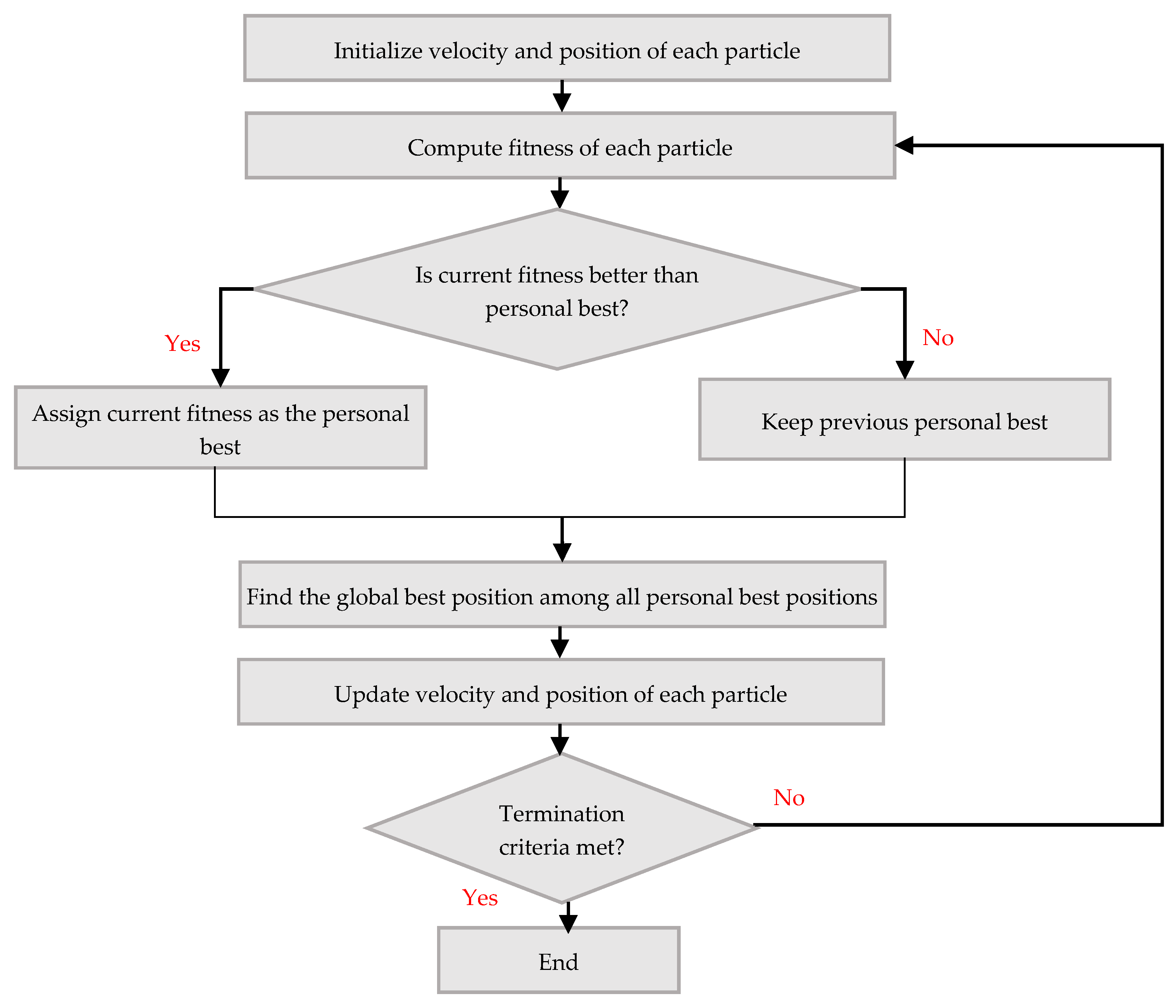
• First, instead of using all extracted features as input, we selected the important features prior to classification. This is the first attempt to use the PSO feature selection algorithm for automated TB detection. By selecting the important features prior to classification, we reduced the noisy and irrelevant features, reduced processing times, and enhanced the prediction performance.
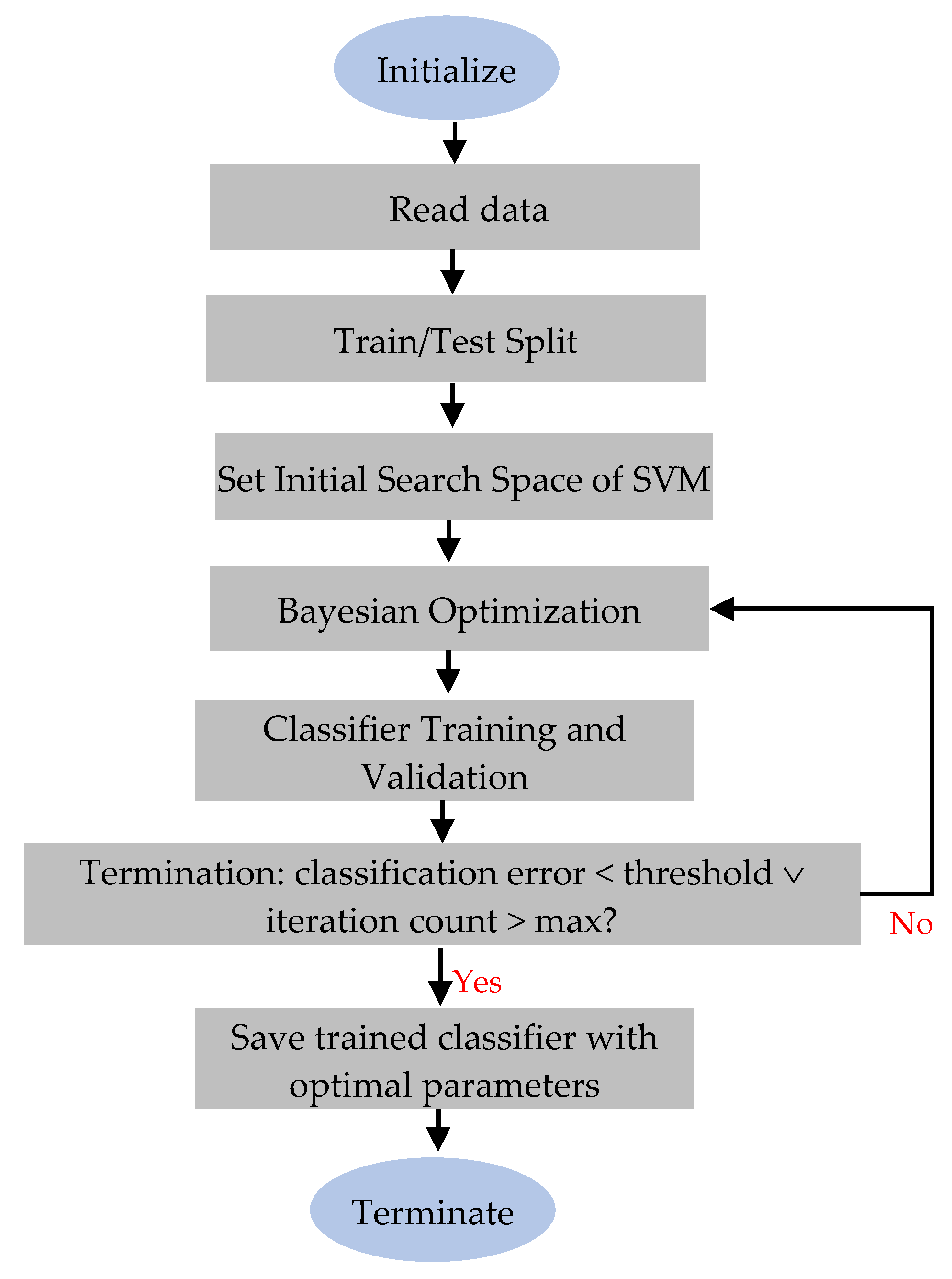
• Second, we optimized an SVM classifier using a Bayesian algorithm.
• Third, we compared the classifications from hand-crafted and deep-activated features using the optimized SVM classifier.
• Fourth, we combined the selected hand-crafted and deep-activated features to generalize the feature set in extensive experiments. To our knowledge, this is the first approach to predict TB using a hybrid feature set which contained a combination of selected handcrafted and deep-activated features. By using the hybrid feature set, we enhanced the prediction performance compared to individual methods and state-of-the-art.

This paper has four sections. Section 2 presents the datasets. Section 3 describes the steps in our method: lung segmentation, feature extraction, feature selection and classification. Section 4 describes and discusses our experimental results. Section 5 concludes and suggests future work.

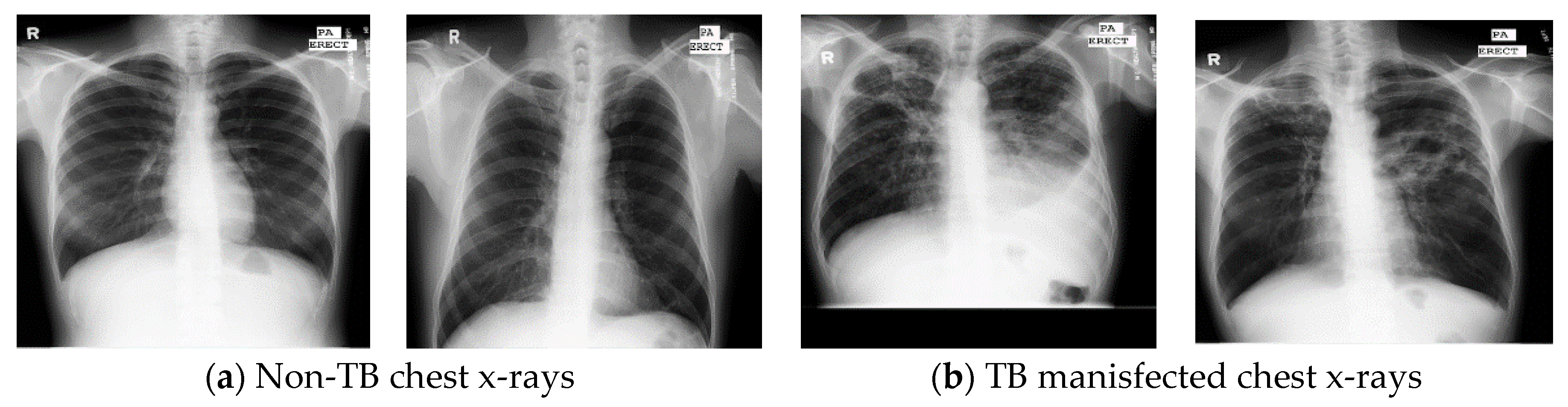
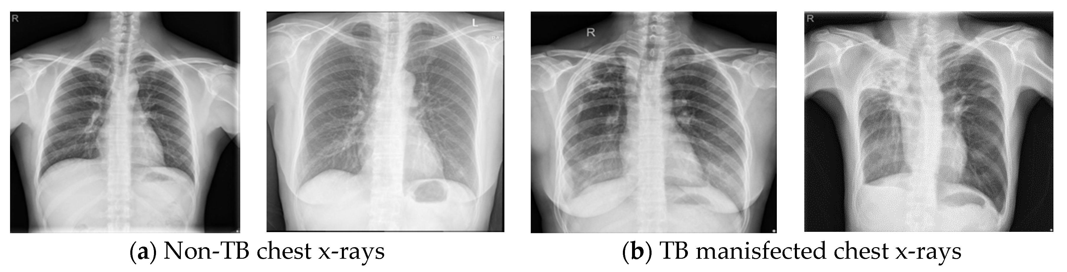
2. Dataset Description

This study used two public datasets: Montgomery (MC) and Shenzhen, published in Jaeger et al. [23]. The MC dataset has 138 frontal chest x-rays—80 normal and 58 show TB; they were collected in Montgomery County, Maryland, USA. The image sizes are 4892 × 4020 or 4020 × 4892. This dataset also has ground truth lung masks for every image and radiological reports describing the lesions. Figure 1 shows example chest x-rays from the MC dataset. The Shenzhen images were collected in the Guandong Hospital, Shenzhen, China; it consists of 326 normal and 336 images containing TB lesions. The image resolutions vary but are approximately 3000 × 3000 pixels. Figure 2 shows some chest-rays in the Shenzhen dataset.

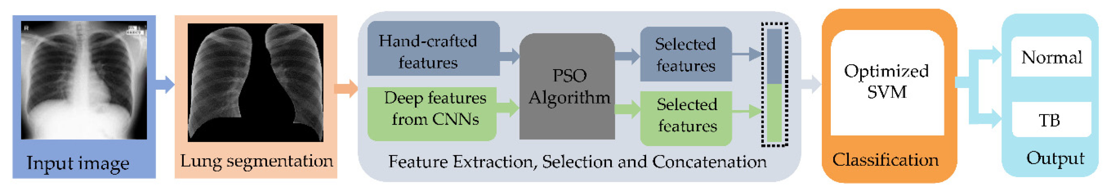
3. Methodology

We aimed to implement an automatic TB screening system using chest x-rays, which could facilitate and expedite TB diagnosis and treatment. Figure 3 depicts the data flow of our algorithm that hybridizes the shallow and deep features for TB classification. It has three main steps: (i) lung segmentation supplemented by preprocessing, (ii) feature extraction, selection and concatenation, and (iii) classification of normal and TB. Each step is presented in details in the following subsections.

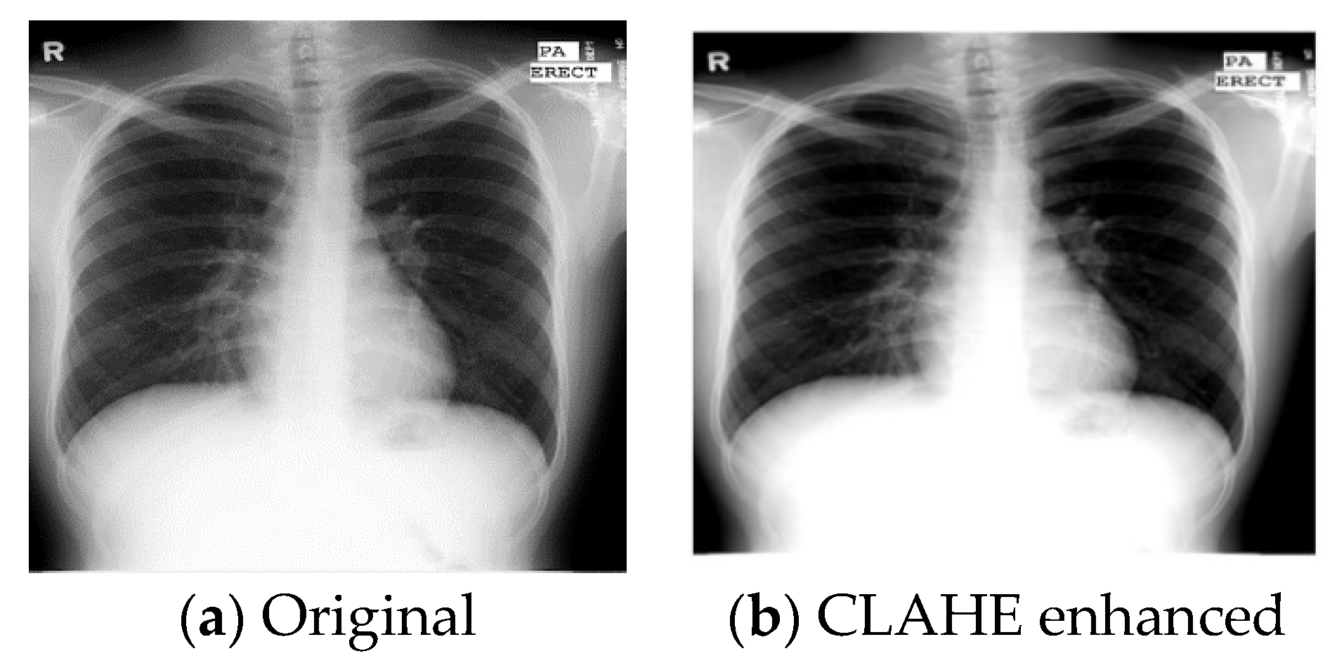
3.1. Preprocessing

The images were resized to a common 512 × 512 pixel size for all images to reduce the processing time. Image enhancement largely influences on the performance of better lung segmentation and classification results [3]. Contrast limited adaptive histogram equalization (CLAHE) is used to improve image quality and contrast [24]. The effect of image enhancement is shown in Figure 4.

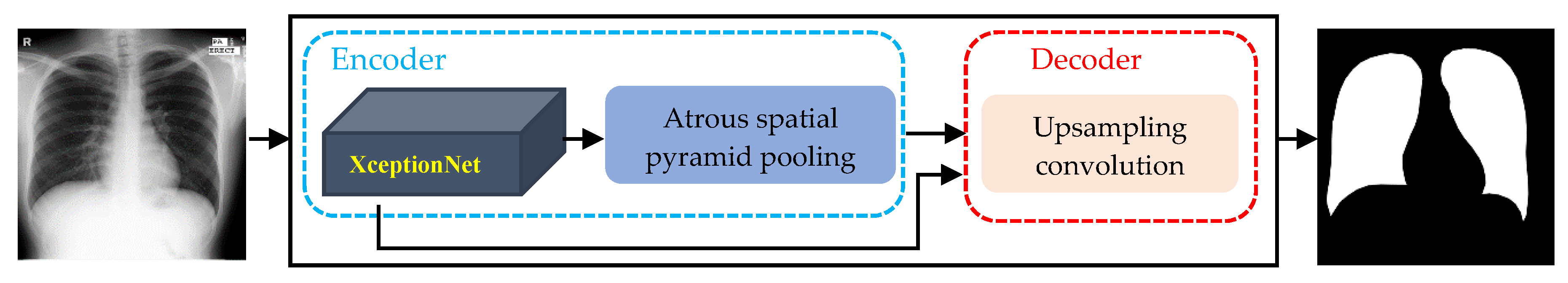
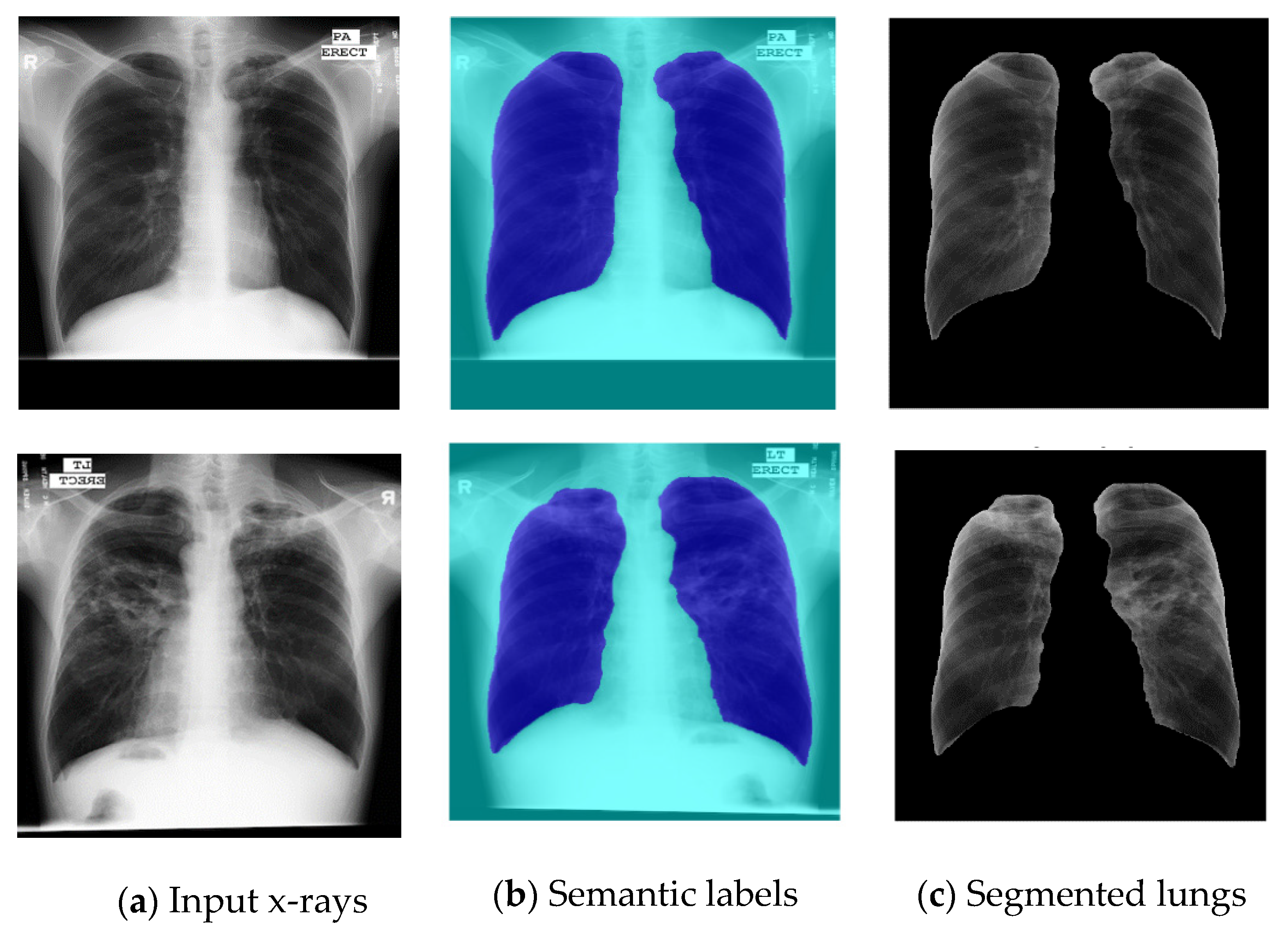
3.2. Lung Segmentation

Lung segmentation is an essential subtask for most disease detection using chest x-rays. Accurate extraction of lung regions impacts the performance of subsequent processes because it defines the region of interest (ROI) where lung abnormalities are searched. Gordienko et al. [25] investigated the impact of lung segmentation and removing bone shadow for lung nodule detection and showed that better accuracy was obtained using the segmented lung and bone shadow removal. Chest x-rays in our study contain the regions other than lungs, which are irrelevant for TB detection. To reduce the risk that the irrelevant regions present in the image mislead the final results, we decided to segregate the lungs. Processing only on the lung regions allows to focus on the useful regions for further processing, thereby improving the algorithm’s performance and lowering the computational time. Previously, we evaluated and compared different lung segmentation methods [26], especially deep semantic ones such as the fully convolutional network (FCN) [27], SegNet [28], U-Net [29] and DeepLabv3+ [30]. The segmentation performance was evaluated at the pixel level by comparing the predicted mask generated by the algorithms with the ground truth mask. Three evaluation metrics namely interception over union (IoU), accuracy and dice similarly coefficient, were measured. We found that DeepLabv3+ [30] with a XceptionNet [31] backbone yielded better segmentation than other methods by achieving IoUs of 95.1% for MC and 92.7% for Shenzen datasets [26]. Inspired by those results, we employed it to segment the lung regions here. The data flow for lung segmentation is depicted in Figure 5. DeepLabv3+ consists of two segments—encoder and decoder. The encoder is to downsample the input images and extract the rich semantic information via atrous spatial pyramid pooling (ASPP) for classification of lung or non-lung pixels. The encoder module employs XceptionNet as a backbone network. XceptionNet is a CNN used for the image classification task. Its architecture is a linear stack of depth-wise separable convolutions with residual connections forming the feature extraction. It has a depth of 126 and constitutes with three components: entry, middle and exit flow. There are a total of 36 convolutional layers to extract the features: 8 in the entry, 24 in the middle and 4 in the exit components [31]. Using the last feature map of XceptionNet, ASPP applied four parallel atrous convolutions with different rates to explore the image-level features at multiple scales. Here we used four different rates of 1, 6, 12 and 18 for atrous convolution. The extracted features maps from atrous convolutions were then pooled into 1 × 1 convolutional feature map, and fed to the decoder module. The decoder module reconstructs the semantic labels by concatenating low and high-level encoder features, followed by upsampling. The decoder module generates the mask for lung regions. We superimposed the lung mask generated by DeepLabv3+ on original chest x-rays to retrieve the segmented lung region. Finally, a morphological gradient operation was used to correct and refine the boundaries of the segmented lungs [32].

3.3. Feature Extraction

Features play a vital role in medical image analysis; they represent the interesting parts of an image in terms of a compact coded attribute. Here, features that will aid TB identification were retrieved and input to classify normal or TB x-rays. The segmented lung regions generated by Section 3.2 were used as input to feature extraction. It would be better if we could use TB lesion region as the ROI. Since there is no labeled dataset that indicates the exact area of TB regions, we could not segment small TB lesions and use them as ROI. We can use either the entire images or the segmented lung regions. As TB lesions appear only on lung region, we used the segmented lung regions as ROIs and extracted the features from them. Two types of features: hand-crafted (shallow) features and deep-activated features from CNNs were extracted. An overview of the applied feature extractors follows.

3.3.1. Hand-Crafted Features

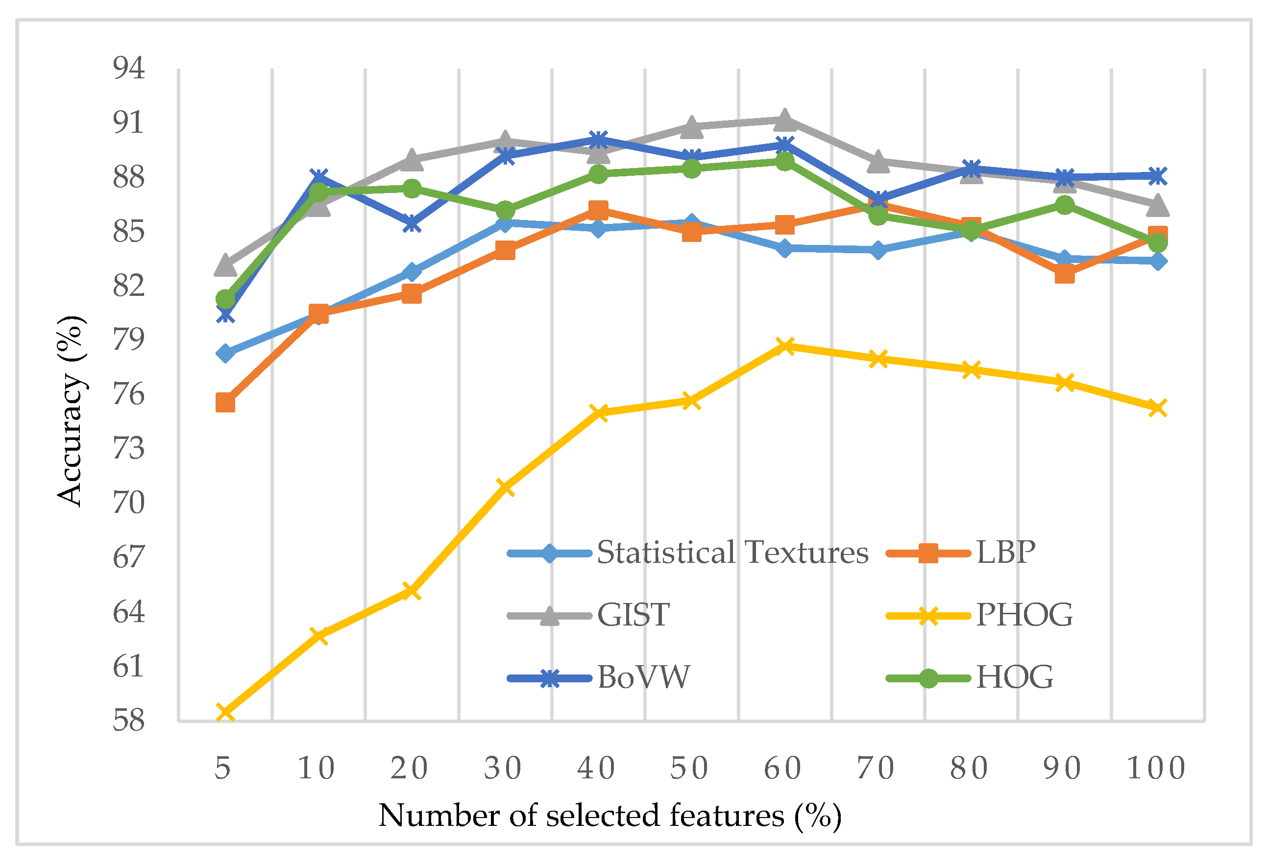
• Statistical textural features: Statistical textural features result from the quantitative analysis of the pixel intensities in the grayscale image using different arrangements. Intensity histograms, first-order statistical textures, gray-level co-occurrence matrices (GLCM) and gray-level run-length matrices (GLRLM) are used as the feature descriptors to extract the statistical textural features. We extracted eight first-order statistical features [33], a total of 88 GLCM features, which encoded 22 different features in four directions [34], and a total of 44 GLRLM features which encoded 11 different features in four directions [35], for a total of 140 textural features.
• Local binary pattern (LBP) features: An LBP is a texture histogram that describes a texture based on differences between central pixels and its neighbors. LBP produces a binary pattern using a threshold value for the central pixel with its neighborhood. A neighbor is 1, when it is greater than or equal to the central pixel, and 0 when it is less. Then the frequency of binary patterns is determined as a histogram of the representative number of binary patterns found in the image [36]. With an 8-pixel neighborhood, 256 features are obtained.
• GIST features: GIST is a feature descriptor that proceeds image filtering to develop a low-level feature set including intensity, color, motion, and orientation based on the information of the gradients, orientations, and scales of the image [37]. GIST captures these features toward identifying the salient image locations that significantly differ from those of the neighbors [14]. First, GIST convolves a given input image with 32 Gabor filters at four different scales and eight different orientations to generate a total of 32 feature maps. Each of these feature maps was then splatted into 16 sub-regions with a 4 × 4 square grid and the feature values within each sub-region were averaged. The averaged values from the 16 sub-regions were concatenated for the 32 different feature maps, resulting in a total of 512 GIST descriptors for a given image.
• Histogram of oriented gradients (HOG) Features: A HOG descriptor, introduced by Dalal and Triggs [38], counts gradient orientation occurrences in localized image regions. HOG measures the first-order image gradient pooled in overlapping orientation bins, and gives a compressed and encoded version of an image. It first computes gradients, creating cell histograms, and generating and normalizing the descriptor blocks. Given an image, HOG first fragments the image into to small-connected regions called cells. Following this, it computes the gradient orientations over each cell and plots a histogram of these orientations, giving the probability for a gradient with a specific orientation in a given path. The adjacent connected cells are grouped into small blocks. The features are extracted over small blocks, in a repetitive fashion, to preserve information about local structures, and the block-wise features are finally integrated into a feature vector. We used the cell size of [16 × 16] pixels, number of bins 3, and 4 × 4 cells in each block. A total of 10,800 HOG features were extracted.
• Pyramid histogram of oriented gradients (PHOG) features: Bosch et al.’s PHOG descriptor [39], represents an image by its spatial layout and local shape. First, PHOG tiles the image into sub-regions, at multiple pyramid-style resolutions, and in each sub-region, the histogram of orientation gradients is applied as a local shape descriptor using the distribution of edge directions. We extracted a total of 168 PHOG features from each image.
• Bag of visual words features: BoVW is a technique adapted from information theory to computer vision applications [40]. Contrary to text, images do not contain words, so, this method creates a bag of features extracted from the images across the classes, using a custom feature descriptor, and constructs a visual vocabulary. First, speeded-up robust features (SURF) [41] are used as feature descriptors to detect interesting key points. Then, k-means clustering [42] is used to generate a visual vocabulary by reducing the dimensions of the features. The center of each cluster refers to a feature or visual word. We extracted 500 BoVW features, using 500 clusters.

A summary of the feature descriptors, along with the number of extracted features, is in

Table 1. Summary of feature descriptors used in our study.

Feature Descriptors		Features	Number of Features
Hand-crafted features	Statistical Textures	First order statistics, GLCM, GLRLM	140
	LBP	Texture histogram	256
	HOG	Occurrences of oriented gradients	10,800
	PHOG	Occurences of oriented gradients at each pyramid resolution level	168
	GIST	Information of the gradients, orientations, and scales of the image	512
	BoVW	Image features as ‘words’	500
Deep CNNs’ Features	Alex	Deep-activated features	1000
	GoogLeNet	Deep-activated features	1000
	InceptionV3	Deep-activated features	1000
	XceptionNet	Deep-activated features	1000
	ResNet-50	Deep-activated features	1000
	SqueezeNet	Deep-activated features	1000
	ShuffleNet	Deep-activated features	1000
	MobileNet	Deep-activated features	1000
	DenseNet	Deep-activated features	1000

.

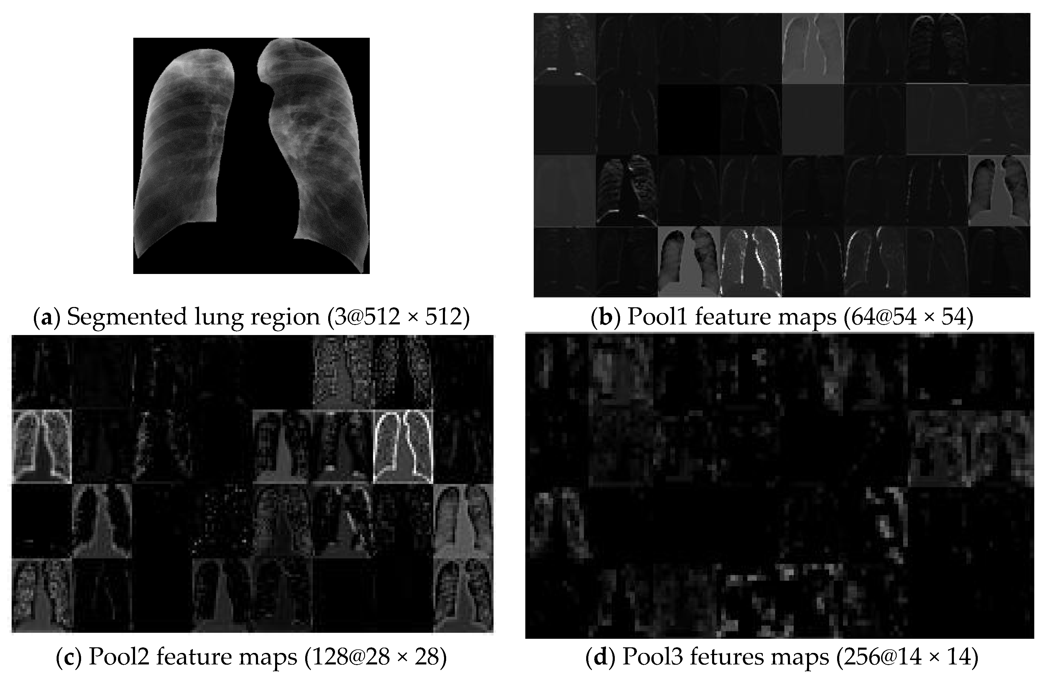
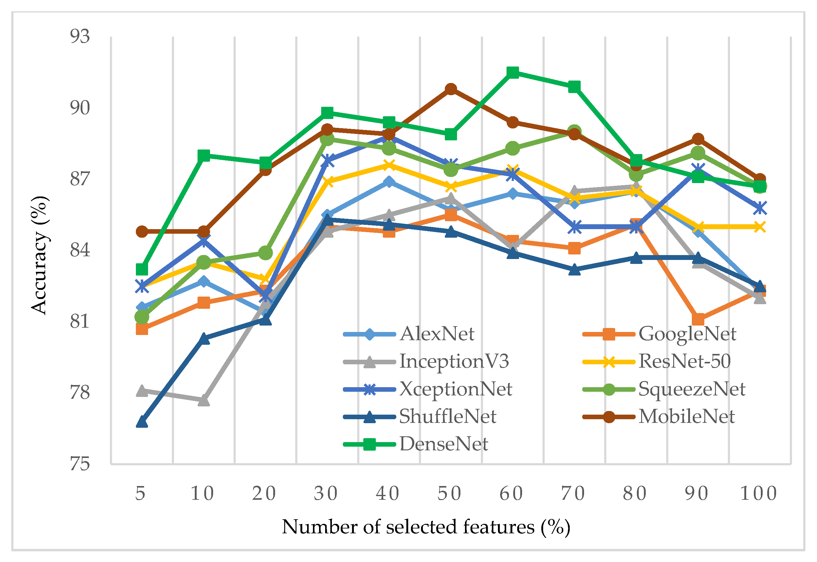
3.3.2. Deep-Activated Features from Pre-trained CNNs

Pre-trained CNNs are convolutional nets, trained on a large datasets and can classify 1000 or more natural objects. There are two ways to use pre-trained CNNs in specific tasks, in our case, medical image classification, transfer learning with fine-tuning as the classifier, and feature extractors along with supervised machine learning classifiers. If there is a limited amount of memory and computational resources, using them as the feature descriptors is a good choice. Here, we used nine different pre-trained CNNs: AlexNet [43], GoogLeNet [44], InceptionV3 [45], XceptionNet [31], ResNet-50 [46], Squeezenet [47], ShuffleNet [48], MobileNet [49] and DenseNet [50], as the feature descriptors to extract high-level deep-activated features. Here, we resized the segmented lung image to the input size, for each CNN, before extracting the features and feeding them to the network. The fully connected layer, which is the last layer before sigmoid classification neuron of each CNN, is retrieved and returns 1000 deep-activated features from each CNN, as listed in Table 1. Pre-trained CNN constructs a hierarchical representation of input images. The early layers extracted fewer low level features. The deep layers extracted high-level features, constructed using earlier layers. Figure 6 displays an example of activated feature maps of three different pooling layers: ‘pool1’, ‘pool2’ and ‘pool3’, of DenseNet. The pooling operation encapsulated the feature maps from convolution layers by highlighting the activated spatial locations, so that the features became more abstract in deeper layers of the CNN. These activation maps reveal the features the CNN learned by overlaying it with the original image.

3.4. Feature Selection

The extracted features include many noisy and irrelevant features. Using those features directly may result in poor classification. Selecting the discriminant features prior to classification is of paramount importance in supervised machine learning methods. The algorithm used for feature selection was a PSO algorithm—a population-based metaheuristic method, inspired by bird flocking or fish swarming, first described by Kennedy and Eberhart [51]. It has been successfully used in global search problems. It is easy to implement, the computation time is reasonable and provides the global search. A PSO flowchart is illustrated in Figure 7. In PSO, each particle has three attributes: position, velocity, and fitness. The position of each particle is a potential solution. The fitness determines the movement of each particle.

Let denote that the population of n particles is $X=\left[X_1, X_2, \dots X_n\right]$ in the potential solution in a D-dimensional space. The position, X_i, and velocity, V_i, of particle, i, are:

$$X_i= \left[x_{i1}, x_{i2}, \dots , x_{iD}\right]$$

(1)

$$V_i= \left[v_{i1}, v_{i2}, \dots , v_{iD}\right]$$

(2)

The particles move through the solution space, and their fitness values are evaluated. The direction and distance of the particle movement is determined by the velocity. The personal best position of each particle and the global best position among all particles are tracked to update individual positions. The personal best position means the best position and fitness found for particle, i: $Pbes{t}_i=\left[p_{i1}, p_{i2}, \dots , p_{iD}\right]$. The global best position, Gbest_, is the best position and fitness for all particles in the swarm. The velocity and position of the particle are updated:

$$v_{id}^{t+1}=\mathsf{\omega }{v}_{id}^t+c_1{r}_1\left(p_{id}^t-x_{id}^t\right)+c_2{r}_2\left(Gbest-x_{id}^t\right),d=1,2,\dots .,D$$

(3)

$$x_{id}^{t+1}=x_{id}^t+v_{id}^{t+1},d=1,2,\dots .,\mathrm{D};i=1,2,\dots \mathrm{n}$$

(4)

where t is the current iteration index, $\omega$ denotes an inertia weight, $c_1$ and $c_2$ are acceleration coefficients, and $r_1$ and $r_2$. are random numbers between 0 and 1.

The features are encoded as the particle swarm here. Pseudocode for feature selection using PSO is given in Algorithm 1. We input the training dataset, the population size, the maximum number of iteration, and objective function. First, particles positions and velocities were randomly initialized and the fitness of each particle was computed using the objective function. The particle with the highest fitness value are considered as the best particle and so, its feature elements will be selected. As our main purpose of optimization is to obtain the higher classification accuracy, we directly used the value of the classification accuracy as the fitness value. The personal and global best positions are tracked to iteratively update the position and velocity of each particle and find the best set of features until a satisfactory fitness or the maximum number of iterations is reached.

Algorithm 1. Pseudo Code 1: PSO based feature selection algorithm

Input: TrainingData, Population, MaximumIteration, ObjectiveFunction

Begin:Randomly intialize position and velocity of particle $x_i$. in the population Set Iteration Counter, t ← 0

Repeat

Compute fitness for each particle using ObjectiveFunction If fitness of $x_i$ > ${\mathit{Pbest}}_i$    ${\mathit{Pbest}}_i\leftarrow x_i$ If fitnest of ${\mathit{Pbest}}_i$ > Gbest    Gbest ←${\mathit{Pbest}}_i$

Begin

Update the velocity and postiion using Equations (3) and (4), respectively

End

Set t ← t+1

Until terminal criteria met finalSet ← finalSet U save(particles)

End

3.5. Classification

A SVM is a supervised learning algorithm, used for classification and regression, originally described by Cortes and Vapnik [52]. An SVM classifies data points of different class by searching for the best hyperplane separating them. Starting with a training dataset, X, comprising I training samples, X = x₁, x₂, …, x_i, and target labels, y = y₁, y₂,…,y_i, where y_i € {−1, +1}, i = [1,2,…,I]. The equation of the linear decision hyperplane, f(x), can be defined:

$$f\left(x\right)=\left(w^T·x\right)+bias$$

(5)

where w is the weight vector or direction of the hyperplane, and bias is the position in the space. To find the best hyperplane of the binary classification of TB and normal, candidate decision surfaces were normalized so that the value of the decision hyperplane f(x) for the support vectors is (w^T · x) + b = +1 for TB class and (w^T · x) + b = −1 for normal class. The best hyperplane is the one with the largest margin between the two classes. The maximum margin between two classes is equivalent to minimizing $\parallel \mathrm{w}{\parallel }^2$. Therefore, the best separating hyperplane is defined:

$$\mathrm{Minimize}:\parallel \mathrm{w}{\parallel }^2$$

(6)

$$\mathrm{subject}\mathrm{to}:y_i\left[\left(w^T·x_i\right)+bias\right]\ge 1, i=1,2,\dots ,I$$

(7)

In a real application, the training data set is not usually linearly separable because some data points may fall inside or behind the margin, or wrong side of the decision hyperplane. Let denote ξ € {ξ₁, ξ₁, ξ_1,…, ξi} as a vector of the error points for I training samples. The decision hyperplane for not linearly separable data is:

$$\mathrm{Minimize}:\parallel \mathrm{w}{\parallel }^2+C{\sum }_{\mathrm{i}=1}^{\mathrm{I}}{\mathsf{\xi }}_i$$

(8)

$$\mathrm{subject}\mathrm{to}:{\mathrm{y}}_{\mathrm{i}}\left[\left(w^T·{\mathrm{x}}_{\mathrm{i}}\right)+bias\right]\ge 1-{\mathsf{\xi }}_i, i =1,2,\dots ,I$$

(9)

where ξ_i=0, 0< ξ_i<1, and ξ_i >1 are error points, C is a penalty parameter used for minimizing the errors falling inside or on the other side of the margin.

When the data is not linearly separable, SVM maps the feature space to a higher dimension using the mapping function or ‘kernel trick’ $\phi$: $K\left(x_j,x_k\right)= <\phi \left(x_j\right),\phi (x_k)>$. Two types of mapping functions, i.e., local (Gaussian radial basis function) and global (linear or polynomial) functions are commonly used for SVM and shown in Equations (10) to (13):

Linear	$$K\left(x_j,x_k\right)=x_j{}^T·x_k$$ (10)
Gaussian radial basis	$$K\left(x_j,x_k\right)=\exp \left(-\gamma \parallel x_j-x_k{\parallel }^2\right),\gamma >0,\gamma =\frac{1}{2{\sigma }^2}$$ (11)
Quadratic polynomial	$$K\left(x_j,x_k\right)={(x_j{}^T·x_k+1)}^2$$ (12)
Cubic polynomial	$$K\left(x_j,x_k\right)={(x_j{}^T·x_k+1)}^3$$ (13)

Using the mapping functions, a non-linear decision surface is defined mathematically:

$$\mathrm{f}\left(\mathrm{x}\right)={\displaystyle \sum }_{i=0}^{S^v}{\alpha }_i{y}_{i }\mathsf{\Phi }\left(x_j\right)·\mathsf{\Phi }\left(x_k\right)+\mathrm{bias}$$

(14)

where S^v denotes the number of support vectors, α_i and y_i, represent the Lagrange multipliers and target labels associated with S^v, respectively. $x_j$. and $x_k$. represent the observations j and k in the training set X [53].

The performance of an SVM relies heavily on the choice of its parameters. Optimal values of the SVM parameters were searched using the Bayesian algorithm [54], as shown in Figure 8. We first defined the initial parameter search space and used the Bayesian method to iteratively search for the optimal values until the maximum criteria reached or the validation accuracy unchanged.

3.6. Evaluation Metrics

We used three metrics to evaluate classification performance: accuracy and F1 Score (F1), formulated in Equations (15) and (16), and area under curve (AUC).

$$Accuracy=\frac{TruePositive+TrueNegative}{TruePositive+FalsePositive+TrueNegative+FalseNegative}\times 100\%$$

(15)

$$F1=\left(2\times \frac{Precision\times Sensitivity}{Precision+Sensitivity}\right)\times 100\%$$

(16)

• TruePositive (TP) refers to the number of TB cases correctly classified as TB.
• TrueNegative (TN) refers to the number of normal cases correctly classified as normal.
• FalsePositive (FP) represents the number of normal cases incorrectly classified as TB.
• FalseNegative (FN) denotes the number of TB cases missed by our method.

Additionally, we rated the classifier, using the Kappa Index [55], which takes all elements in the confusion matrix into account, whereas accuracy counts only those on the main diagonal. The Kappa Index was computed:

$$Kappa Index=\frac{\left(P_{observed}-P_{expected}\right)}{1-P_{expected}}\times 100\%$$

(17)

$P_{observed}$ is the observational probability of agreement, $P_{observed}=\frac{TP+TN}{TP+TN+FP+FN}$, and $P_{expected}$ is the expected probability of agreement,$P_{e\mathrm{x}pected}=\frac{\left(TN+FP\right)·\left(TN+FN\right)+\left(TP+FP\right)·\left(TP+FN\right)}{{\left(TP+TN+FP+FN\right)}^2}$. Classification performance based on Kappa Index values is shown in

Table 2. Quality of classification evaluated by Kappa Index.

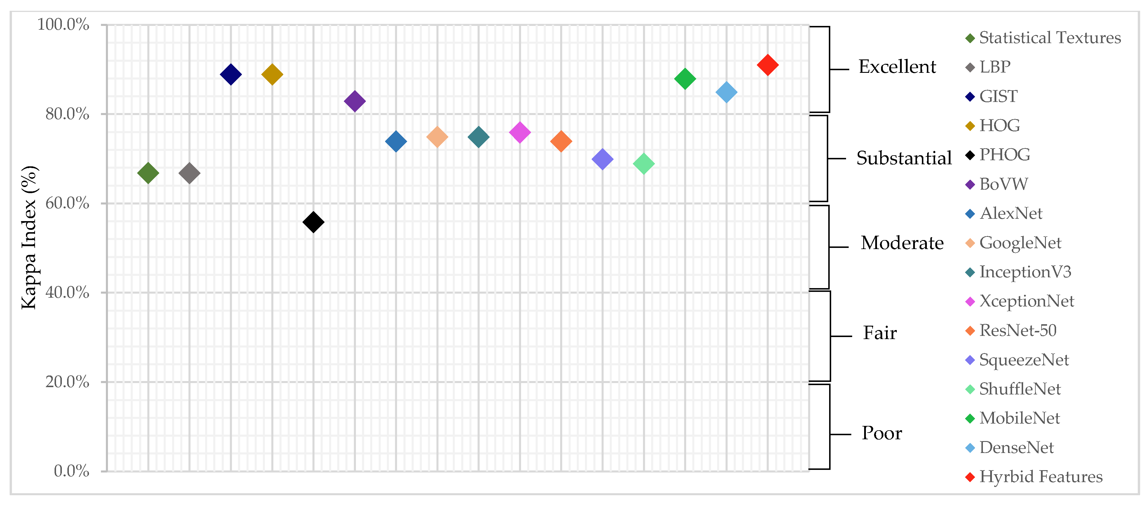
Kappa Index	Quality
<0	Poor
0–20	Slight
21–40	Fair
41–60	Moderate
61–80	Substantial
81–100	Excellent

, as defined by Landis and Koch [56].

4. Experimental Results and Discussion

Experiments were run in MATLAB_R2019b using a 9th Generation Core i7 at 3.0 GHz CPU and Nvidia T1660Ti GPU under Windows 10. Two public datasets: MC and Shenzen were used. The datasets were randomly split into training (70%) and testing (30%). Since the MC dataset is limited, the training sets from both datasets were combined to generate the combined training set and used to develop and select algorithms. The testing sets were used to assess the performance. First, we segregated the lung regions, using DeepLabv3+ with the XceptionNet backbone. Segmentation performance is described in our previous study [25]. Example lung segmentations are in Figure 9.

Once the lung regions were retrieved, we extracted six sets of hand-crafted features: statistical textures, LBP, GIST, HOG, PHOG, and BoVW, and nine sets of deep-activated features from nine different pre-trained CNNS: AlexNet, GoogLeNet, InceptionV3, XceptionNet, ResNet-50, SqueezeNet, ShuffleNet, MobileNet and DenseNet. Then, we used a PSO based feature selection algorithm to select the dominant features from each feature set. From each dataset, we selected 5%, 10%, 20%, 30%, 40%, 50%, 60%, 70%, 80%, 90% and 100% (all features) of the features and 11 different selected percentages multiplied by 15 different feature sets—a total of 165 tests were performed. The performance of the selected feature subset was assessed using linear SVM. The accuracy for the different feature sets with a corresponding selected feature is plotted in Figure 10 for hand-crafted and in Figure 11 for deep-activated features. We found that selecting small numbers of features, up to 20% of the total, delivered poor accuracy. Conversely, selecting a large number of features, from 80% to 100% of the total, caused a drop in accuracy. Selecting 30–70% of the features provided better accuracy. Thus, we selected an average 50% of the features from each feature set. Each selected feature subset was separately fed to an SVM classifier to predict TB.

To obtain a robust and effective SVM, it is crucial to select suitable parameters, e.g., penalty parameter (C), kernel functions and kernel scales. First, we defined the parameter search spaces: C = {0.001, 1000}, kernel functions = {Linear, Gaussian, Quadratic, Cubic}, and kernel scale, $\gamma$ = {0.001–1000}, and used a Bayesian algorithm to find the optimal parameters for each feature set. The optimal parameters for each feature set are listed in

Table 3. The optimal hyper parameters of SVM for each feature set.

Feature Sets		Penalty Term (C)	Kernel Functions	Kernel Scale $\left(\mathit{\gamma }\right)$
Hand-crafted features	Statistical Textures	8.58 × 100	Linear	N/A
	LBP	9.24 × 10−3	Linear	N/A
	HOG	8.28 × 102	Gaussian	8.21 × 102
	GIST	9.96 × 102	Gaussian	3.10 × 101
	PHOG	2.58 × 100	Gaussian	3.37 × 101
	BoVW	3.64 × 10−3	Linear	N/A
Deep-activated features	AlexNet	9.87 × 102	Gaussian	6.08 × 102
	GoogLeNet	5.51 × 10−2	Linear	N/A
	InceptionV3	1.77 × 10−2	Linear	N/A
	XceptionNet	1.01 × 10−3	Linear	NaN
	ResNet-50	9.98 × 102	Gaussian	9.91 × 102
	SqueezeNet	2.02 × 10−2	Linear	N/A
	ShuffleNet	1.00 × 10−3	Linear	N/A
	MobileNet	3.05 × 102	Gaussian	3.01 × 101
	DenseNet	5.60 × 102	Gaussian	7.32 × 102

Note: N/A= not applicable.

. We trained 15 SVM classifiers with the parameters in Table 3. Once the optimized SVM classifiers were trained, we used them to identify TB. The classification metrics were F1, Accuracy, AUC, and Kappa Index.

Table 4. Performance of each individual set and hybrid feature using the optimized SVM classifiers—MC dataset.

Features	F1 (%)	Accuracy (%)	AUC (%)
Statistical Textures	81.8	80.5	87.9
LBP	79.2	73.2	86.2
GIST	90.9	90.2	93.1
HOG	93.3	92.7	100.0
PHOG	75.6	73.2	83.6
BoVW	91.3	90.2	99.8
AlexNet	76.9	70.7	85.7
GoogLeNet	88.9	87.8	91.9
InceptionV3	83.7	82.9	89.0
XceptionNet	85.7	82.9	91.0
ResNet-50	81.8	80.5	88.8
SqueezeNet	81.6	78.0	79.5
ShuffleNet	83.3	80.5	84.0
MobileNet	90.9	90.2	93.1
DenseNet	93.3	92.7	99.5
Hybrid features (GIST+HOG+BoVW+MobileNet+DenseNet)	93.3	92.7	99.5

and

Table 5. Performance for individual set and hybrid feature using the optimized SVM classifiers—Shenzhen dataset.

Features	F1 (%)	Accuracy (%)	AUC (%)
Statistical Textures	83.1	83.4	91.0
LBP	83.4	83.4	90.7
GIST	94.4	94.5	98.6
HOG	94.5	94.5	96.7
PHOG	78.8	77.9	85.9
BoVW	91.5	91.5	95.7
AlexNet	86.6	86.9	94.0
GoogLeNet	87.3	87.4	93.3
InceptionV3	87.3	87.4	94.1
XceptionNet	88.0	87.9	94.4
ResNet-50	85.7	85.9	94.0
SqueezeNet	85.0	84.9	90.1
ShuffleNet	84.7	84.4	88.9
MobileNet	93.9	94.0	98.6
DenseNet	92.5	92.5	97.8
Hybrid features (GIST+HOG+BoVW+MobileNet+DenseNet)	95.4	95.5	99.5

listed the F1, accuracy and AUC using 15 different methods for MC and Shenzen datasets. Figure 12 and Figure 13 plot and show the performance of each method for the MC and Shenzen datasets We found that GIST, HOG, BoVW from hand-crafted features, and MobileNet and DenseNet from pre-trained CNN performed better than other methods for both datasets, achieving over 90% of F1, Accuracy, and AUC with an excellent Kappa (over 80%). To improve prediction, we combined the five best-performing feature subsets: GIST, HOG, BoVW, MobileNet and DenseNet and built a hybrid feature set that contained local and global texture features and high-level deep activated features. The hybrid feature set contained 50% of the selected features of five feature sets: 256 GIST features, 5400 HOG features, 250 BoVW features, 500 MobileNet features and 500 DenseNet features, and fed them as input to SVM classifier. The performance of the SVM classifier using the hybrid feature set is in Table 4 for MC and Table 5 for Shenzen datasets. Its Kappa indices are plotted in Figure 12 and Figure 13. It achieved favorable performance with 93.3% F1, 92.7% accuracy, 99.5% AUC for MC and 95.4% F1, 95.5% accuracy, 99.5% AUC for Shenzhen. Its Kappa was ‘excellent’ for both datasets. The hybrid feature set marginally improved the prediction compared to individual best-performing feature sets on Shenzen dataset while matching the best prediction made by HOG and DenseNet feature sets using the MC dataset.

We compared our method with previous studies in

Table 6. Performance of previous studies and our method using MC and Shenzhen datasets.

Authors	Methods Used	MC		Shenzhen
		Accuracy	AUC	Accuracy	AUC
Jaeger et al. [7]	▪ Lung segmentation using optimized graph cuts ▪ Multiple local and global hand-crafted features ▪ SVM classifier	78.3%	86.9%	84.0%	90.0%
Vajda et al. [8]	▪ Atlas-driven lung segmentation ▪ Multi-level features of shape, curvature and eigenvalues of the Hessian matrix ▪ Wrapper feature selection with MLP	78.3%	76.0%	95.6%	99.0%
Karargyris et al. [9]	▪ Atlas-driven lung segmentation ▪ Combination of texture and shape ▪ SVM	NA	NA	NA	93.4%
Jemal [10]	▪ Lung segmentation using thresholding ▪ Textural features ▪ SVM classifier	68.1%	71.0%	83.4%	91.0%
Santosh et al. [11]	▪ Multi-scale features of shape, edge, and texture ▪ A combination of a Bayes network, MLP and random forest	83.0%	90.0%	91.0%	96.0%
Pasa et al. [17]	▪ A variant of AlexNet architecture	79.0%	81.1%	84.4%	90.0%
Hwang et al. [18]	▪ Pre-trained AlexNet	67.4%	88.4%	83.7%	92.6%
Islam et al. [19]	▪ Ensemble of pre-trained CNNs	NA	NA	NA	94%
Lopes et al. [21]	▪ Features from GoogLeNet, ResNet, and VGGNet ▪ SVM	82.6%	92.6%	84.7%	92.6%
Rajaraman et al. [22]	▪ Atlas-based method ▪ A stacked model of hand-crafted features and CNNs	87.5%	98.6%	95.9%	99.4%
Our method	▪ Lung segmentation using DeepLabv3+ ▪ PSO based feature selection ▪ Hybrid feature set of selected GIST, HOG, BoVW, MobileNet and DenseNet features ▪ Optimized SVM classifier	92.7%	99.5%	95.5%	99.5%

. Our method surpassed the existing studies for the MC dataset with accuracy 92.7% and AUC 99.5%, and obtained comparable results with the state of the art for the Shenzen dataset with accuracy 95.9% and AUC 99.5%. From Table 6, we found that the methods produced better performance on Shenzhen dataset compared to MC dataset. The same pattern is seen Table 4 and Table 5 of our study, and also in related works [7,8,10,11,17,18,21,22]. The lower performance with the smaller MC dataset is probably attributed to its limited size containing only 138 x-rays, and therefore lower range of samples to be trained and learnt. Shenzhen dataset is larger than MC dataset where the number of samples is over 300, both for normal and TB cases. Another factor of impairing the classification accuracy could be the unbalanced data distribution. The MC dataset is unbalanced, with a smaller number of TB cases while the Shenzen set is larger and balanced with almost 50% TB cases. It is also noteworthy that the most hand-crafted used here have already been studied. However, they were directly input to the classifier. On the other hand, our method, first filtered out the noisy and irrelevant features and selected the dominant features. For deep-activated features, few pre-trained CNNs were used in previous studies, whereas we studied a wide variety of different CNN structures. We also first selected the important deep activated features, before feeding them to the classifier. Rajaraman et al. [22] used hand-crafted based classifiers and pre-trained CNNs separately and, combined their results via majority voting to make a final decision. Here, we made alternative use of these features. Our method first selected the important features and hybridized the best-performing shallow hand-crafted features and high-level deep features, so that the classifier had better information to make the prediction. Achieving the better results than the previous studies using the same feature sets was due to the feature selection. Using a PSO feature selection and hybridizing the hand-crafted and deep-activated features were the keys to improved prediction. The code supporting the findings of this study are available from the corresponding authors upon request.

5. Conclusions

We present a technique for learning with a hybrid of hand-crafted features and deep-activated features from pre-trained CNNs, with help of a PSO algorithm and an optimized SVM classifier. We initially preprocessed the images using CLAHE and subsequently segmented the lung regions using a deep semantic segmentation technique, which used XceptionNet as the backbone in DeepLabv3+. From the segmented lung regions, we extracted six sets of hand-crafted features using statistical textures, LBP, GIST, HOG, PHOG, and BoVW feature descriptors. Then, we used nine pre-trained CNNs as the feature descriptors to retrieve the deep-activated features. To select the important features from each feature set, a PSO based feature selection algorithm selected different fractions of features. A total of 50% of selected features were input to the optimized SVM classifier. Additionally, 15 features sets were tested, but GIST, HOG, BoVW, MobileNet, and DenseNet features performed better than the rest. To build a classifier that learnt from both local and global hand-crafted features, as well as high-level deep-activated features, we combined the five-best performing feature sets into a hybrid feature set and input it to the classifier to identify TB. The SVM classifier, using the hybrid feature set, obtained 92.7% accuracy, 99.5% AUC for the MC and 95.5% accuracy, 99.5% AUC for the Shenzen dataset, and achieved an excellent Kappa Index for both datasets. Our results surpassed those in previous studies for the MC dataset and matched them for the Shenzen dataset. Using a PSO feature selection method and a hybrid feature set was a key to improved prediction.

We here used a PSO algorithm to rank the importance of the features and select the different fractions of features. It is a drawback and time-consuming that we have to run exhausting tests to find the optimal number for selecting the features. Therefore, we will work on the feature selection algorithm, which will automatically find the optimal number of features itself. Besides, to test the robustness of the existing algorithms or developing a new algorithm, large number of images are required. As the acquisition and labelling of medical images are expensive, we have a great interest of using synthesis images generated by generative adversarial networks for training deep learning models which require large number of training images. In this way, we could develop even more robust TB classifier.

References

- World Health Organization. Global Tuberculosis Report 2019. Available online: https://www.who.int/tb/publications/global_report/en/ (accessed on 25 February 2020).
- Suleiman, K.; Lessem, E. AN ACTIVIST’S. GUIDE TO “Tuberculosis Diagnostic Tools”; Treatment Action Group: New York, NY, USA, 2017. [Google Scholar]
- Qin, C.; Yao, D.; Shi, Y.; Song, Z. Computer-aided detection in chest radiography based on artificial intelligence: A survey. Biomed. Eng. Online 2018, 17, 113. [Google Scholar] [CrossRef] [Green Version]
- Van Ginneken, B.; Katsuragawa, S.; Romeny, B.M.T.H.; Doi, K.; Viergever, M.A. Automatic detection of abnormalities in chest radiographs using local texture analysis. IEEE Trans. Med. Imaging 2002, 21, 139–149. [Google Scholar] [CrossRef]
- Hogeweg, L.; Mol, C.; de Jong, P.A.; Dawson, R.; Ayles, H.; van Ginneken, B. Fusion of local and global detection systems to detect tuberculosis in chest radiographs. In Proceedings of the International Conference on Medical Image Computing and Computer-Assisted Intervention 2010, Beijing, China, 20–24 September 2010; Springer: Berlin/Heidelberg, Germany; pp. 650–657. [Google Scholar]
- Tan, J.H.; Acharya, U.R.; Tan, C.; Abraham, K.T.; Lim, C.M. Computer-assisted diagnosis of tuberculosis: A first order statistical approach to chest radiograph. J. Med. Syst. 2012, 36, 2751–2759. [Google Scholar] [CrossRef] [PubMed]
- Jaeger, S.; Karargyris, A.; Candemir, S.; Folio, L.; Siegelman, J.; Callaghan, F.; Xue, Z.; Palaniappan, K.; Singh, R.K.; Antani, S.; et al. Automatic tuberculosis screening using chest radiographs. IEEE Trans. Med. Imaging 2013, 33, 233–245. [Google Scholar] [CrossRef] [PubMed]
- Vajda, S.; Karargyris, A.; Jaeger, S.; Santosh, K.C.; Candemir, S.; Xue, Z.; Antani, S.; Thoma, G. Feature selection for automatic tuberculosis screening in frontal chest radiographs. J. Med. Syst. 2018, 42, 146. [Google Scholar] [CrossRef] [PubMed]
- Karargyris, A.; Siegelman, J.; Tzortzis, D.; Jaeger, S.; Candemir, S.; Xue, Z.; Santosh, K.C.; Vajda, S.; Antani, S.; Folio, L.; et al. Combination of texture and shape features to detect pulmonary abnormalities in digital chest X-rays. Int. J. Comput. Assist. Radiol. Surg. 2016, 11, 99–106. [Google Scholar] [CrossRef] [PubMed]
- Jemal, A. Lung Tuberculosis Detection Model in Thorax Radiography. Master’s Thesis, Department of Computing, Adama Science and Technology University, Adama, Ethiopia, 2019. [Google Scholar]
- Santosh, K.C.; Antani, S. Automated chest X-ray screening: Can lung region symmetry help detect pulmonary abnormalities? IEEE Trans. Med. Imaging 2017, 37, 1168–1177. [Google Scholar] [CrossRef]
- Melendez, J.; Van Ginneken, B.; Maduskar, P.; Philipsen, R.H.; Reither, K.; Breuninger, M.; Adetifa, I.M.; Maane, R.; Ayles, H.; Sánchez, C.I. A novel multiple-instance learning-based approach to computer-aided detection of tuberculosis on chest x-rays. IEEE Trans. Med. Imaging 2014, 34, 179–192. [Google Scholar] [CrossRef]
- Melendez, J.; Sánchez, C.I.; Philipsen, R.H.; Maduskar, P.; Dawson, R.; Theron, G.; Dheda, K.; Van Ginneken, B. An automated tuberculosis screening strategy combining X-ray-based computer-aided detection and clinical information. Sci. Rep. 2016, 6, 25265. [Google Scholar] [CrossRef]
- Chauhan, A.; Chauhan, D.; Rout, C. Role of GIST and PHOG features in computer-aided diagnosis of tuberculosis without segmentation. PLoS ONE 2014, 9, e112980. [Google Scholar] [CrossRef]
- Esteva, A.; Kuprel, B.; Novoa, R.A.; Ko, J.; Swetter, S.M.; Blau, H.M.; Thrun, S. Dermatologist-level classification of skin cancer with deep neural networks. Nature 2017, 542, 115–118. [Google Scholar] [CrossRef] [PubMed]
- Rajpurkar, P.; Irvin, J.; Zhu, K.; Yang, B.; Mehta, H.; Duan, T.; Ding, D.; Bagul, A.; Langlotz, C.; Lungren, M.P.; et al. Radiologist-level pneumonia detection on chest x-rays with deep learning. arXiv 2017, arXiv:1711.05225. [Google Scholar]
- Pasa, F.; Golkov, V.; Pfeiffer, F.; Cremers, D.; Pfeiffer, D. Efficient deep network architectures for fast chest x-ray tuberculosis screening and visualization. Sci. Rep. 2019, 9, 6268. [Google Scholar] [CrossRef] [PubMed] [Green Version]
- Hwang, S.; Kim, H.; Jeong, J.; Kim, H. A Novel Approach for Tuberculosis Screening Based on Deep Convolutional Neural Networks. In Proceedings of the SPIE—The International Society for Optical Engineering, Medical Imaging 2016: Computer-Aided Diagnosis, San Diego, CA, USA, 28 February–3 March 2016; Volume 9785, p. 97852W. [Google Scholar]
- Islam, M.T.; Aowal, M.A.; Minhaz, A.T.; Ashraf, K. Abnormality Detection and Localization in Chest X-Rays using Deep Convolutional Neural Networks. arXiv 2017, arXiv:1705.09850. [Google Scholar]
- Lakhani, P.; Sundaram, B. Deep learning at chest radiography: Automated classification of pulmonary tuberculosis by using convolutional neural networks. Radiology 2017, 284, 574–582. [Google Scholar] [CrossRef]
- Lopes, U.K.; Valiati, J.F. Pre-trained convolutional neural networks as feature extractors for tuberculosis detection. Comput. Biol. Med. 2017, 89, 135–143. [Google Scholar] [CrossRef]
- Rajaraman, S.; Cemir, S.; Xue, Z.; Alderson, P.; Thoma, G.; Antani, S. A Novel Stacked Model Ensemble for Improved TB Detection in Chest Radiographs. In Medical Imaging: Artificial Intelligence, Image Recognition, and Machine Learning Techniques; CRC Press: Boca Raton, FL, USA, 2019; pp. 1–26. [Google Scholar]
- Jaeger, S.; Candemir, S.; Antani, S.; Wáng, Y.X.J.; Lu, P.X.; Thoma, G. Two public chest x-ray datasets for computer-aided screening of pulmonary diseases. Quant. Imaging Med. Surg. 2014, 4, 475–477. [Google Scholar]
- Zuiderveld, K. Contrast limited adaptive histogram equalization. In Graphics Gems IV; Academic Press Professional Inc.: Cambridge, MA, USA, 1994; pp. 474–485. [Google Scholar]
- Gordienko, Y.; Gang, P.; Hui, J.; Zeng, W.; Kochura, Y.; Alienin, O.; Rokovyi, O.; Stirenko, S. Deep learning with lung segmentation and bone shadow exclusion techniques for chest X-ray analysis of lung cancer. In International Conference on Theory and Applications of Fuzzy Systems and Soft Computing; Springer: New York, NY, USA, 2018; pp. 638–647. [Google Scholar]
- Win, K.Y.; Maneerat, N.; Hamamoto, K.; Syna, S. A cascade of encoder-decoder with atrous separable convolution and ensemble deep convolutional neural networks for Tuberculosis detection. IEEE Access 2020. under review. [Google Scholar]
- Long, J.; Shelhamer, E.; Darrell, T. Fully Convolutional Networks for Semantic Segmentation. In Proceedings of the IEEE Conference on Computer Vision and Pattern Recognition (CVPR), Boston, MA, USA, 7–12 June 2015; pp. 3431–3440. [Google Scholar]
- Badrinarayanan, V.; Kendall, A.; Cipolla, R. Segnet: A Deep Convolutional Encoder-Decoder Architecture for Image Segmentation. arXiv 2015, arXiv:1511.0051. [Google Scholar] [CrossRef]
- Ronneberger, O.; Fischer, P.; Brox, T. U-Net: Convolutional Networks for Biomedical Image Segmentation. In Proceedings of the International Conference on Medical Image Computing and Computer-Assisted Intervention, Munich, Germany, 5–9 October 2015; Volume 9351, pp. 234–241. [Google Scholar]
- Chen, L.C.; Zhu, Y.; Papandreou, G.; Schroff, F.; Adam, H. Encoder-decoder with atrous separable convolution for semantic image segmentation. In Proceedings of the ECCV: European Conference on Computer Vision, Munich, Germany, 8–14 September 2018; pp. 801–818. [Google Scholar]
- Chollet, F. Xception: Deep learning with depthwise separable convolutions. In Proceedings of the IEEE Conference on Computer Vision and Pattern Recognition, Honolulu, HI, USA, 21–26 July 2017; pp. 1251–1258. [Google Scholar]
- Soille, P. Morphological Image Analysis: Principles and Applications; Springer Science & Business Media: Berlin, Germany, 2013. [Google Scholar]
- Srinivasan, G.N.; Shobha, G. Statistical texture analysis. Int. J. Comput. Inf. Eng. 2008, 36, 1264–1269. [Google Scholar]
- Haralick, R.M.; Shanmugam, K.; Dinstein, I. Textural features for image classi cation. IEEE Trans. Syst. Man Cybern. 1973, 3, 610–621. [Google Scholar] [CrossRef] [Green Version]
- Dasarathy, B.V.; Holder, E.B. Image characterizations based on joint gray level-run length distributions. Pattern Recognit. Lett. 1991, 12, 497–502. [Google Scholar] [CrossRef]
- Ojala, T.; Pietikainen, M.; Maenpaa, T. Multiresolution Gray Scale and Rotation Invariant Texture Classification with Local Binary Patterns. IEEE Trans. Pattern Anal. Mach. Intell. 2002, 24, 971–987. [Google Scholar] [CrossRef]
- Grigorescu, S.E.; Petkov, N.; Kruizinga, P. Comparison of texture features based on Gabor filters. IEEE Trans. Image Process. 2002, 11, 1160–1167. [Google Scholar] [CrossRef] [PubMed] [Green Version]
- Dalal, N.; Triggs, W. Histograms of oriented gradients for human detection. In Proceedings of the 2005 IEEE Computer Society Conference on Computer Vision and Pattern Recognition CVPR05, San Diego, CA, USA, 20–25 June 2005; Volume 1, pp. 886–893. [Google Scholar]
- Bosch, A.; Zisserman, A.; Munoz, X. Representing shape with a spatial pyramid kernel. In Proceedings of the 6th ACM international conference on Image and video retrieval, Amsterdam, The Netherlands, 9–11 July 2007; pp. 401–408. [Google Scholar]
- Csurka, G.; Dance, C.R.; Fan, L.; Willamowski, J.; Bray, C. Visual Categorization with Bags of Keypoints. In Workshop on Statistical Learning in Computer Vision, ECCV, Proceedings of the European Conference on Computer Vision, Prague, Czech Republic, 11–14 May 2004; Springer: Berlin/Heidelberg, Germany, 2004; pp. 1–22. [Google Scholar]
- Bay, H.; Ess, A.; Tuytelaars, T.; Van Gool, L. SURF: Speeded Up Robust Features. Comput. Vis. Image Underst. (CVIU) 2008, 110, 346–359. [Google Scholar] [CrossRef]
- Arthur, D.; Vassilvitskii, S. K-means++: The Advantages of Careful Seeding. In Proceedings of the Eighteenth Annual ACM-SIAM Symposium on Discrete Algorithms, New Orleans, LA, USA, 7–9 January 2007; pp. 1027–1035. [Google Scholar]
- Krizhevsky, A.; Sutskever, I.; Hinton, G.E. Imagenet classification with deep convolutional neural networks. In Proceedings of the 26th Annual Conference on Neural Information Processing Systems, Lake Tahoe, NV, USA, 3–6 December 2012; pp. 1097–1105. [Google Scholar]
- Szegedy, C.; Liu, W.; Jia, Y.; Sermanet, P.; Reed, S.; Anguelov, D.; Erhan, D.; Vanhoucke, V.; Rabinovich, A. Going deeper with convolutions. In Proceedings of the IEEE Conference on Computer Vision and Pattern Recognition, Boston, MA, USA, 7–12 June 2015; pp. 1–9. [Google Scholar]
- Szegedy, C.; Vanhoucke, V.; Ioffe, S.; Shlens, J.; Wojna, Z. Rethinking the inception architecture for computer vision. In Proceedings of the IEEE Conference on Computer Vision and Pattern Recognition, Las Vegas, NV, USA, 27–30 June 2016; pp. 2818–2826. [Google Scholar]
- He, K.; Zhang, X.; Ren, S.; Sun, J. Deep residual learning for image recognition. In Proceedings of the IEEE Conference on Computer Vision and Pattern Recognition, Las Vegas, NV, USA, 27–30 June 2016; pp. 770–778. [Google Scholar]
- Iandola, F.N.; Han, S.; Moskewicz, M.W.; Ashraf, K.; Dally, W.J.; Keutzer, K. SqueezeNet: AlexNet-level accuracy with 50x fewer parameters and <0.5 MB model size. arXiv 2016, arXiv:1602.07360. [Google Scholar]
- Zhang, X.; Zhou, X.; Lin, M.; Sun, J. Shufflenet: An extremely efficient convolutional neural network for mobile devices. In Proceedings of the IEEE Conference on Computer Vision and Pattern Recognition, Salt Lake City, UT, USA, 18–23 June 2018; pp. 6848–6856. [Google Scholar]
- Sandler, M.; Howard, A.; Zhu, M.; Zhmoginov, A.; Chen, L.C. Mobilenetv2: Inverted residuals and linear bottlenecks. In Proceedings of the IEEE Conference on Computer Vision and Pattern Recognition, Salt Lake City, UT, USA, 18–23 June 2018; pp. 4510–4520. [Google Scholar]
- Huang, G.; Liu, Z.; Van Der Maaten, L.; Weinberger, K.Q. Densely connected convolutional networks. In Proceedings of the IEEE Conference on Computer Vision and Pattern Recognition, Honolulu, HI, USA, 21–26 July 2017; pp. 4700–4708. [Google Scholar]
- Kennedy, J.; Eberhart, R. Particle swarm optimization. In Proceedings of the IEEE International Conference on Neural Networks, Perth, Australia, 27 November–1 December 1995; pp. 1942–1948, 1995. [Google Scholar]
- Cortes, C.; Vapnik, V. Support-vector networks. Mach. Learn. 1995, 20, 273–297. [Google Scholar]
- Christianini, N.; Shawe-Taylor, J.C. An. Introduction to Support. Vector Machines and Other Kernel-Based Learning Methods; Cambridge University Press: Cambridge, UK, 2000. [Google Scholar]
- Snoek, J.; Larochelle, H.; Adams, R.P. Practical Bayesian Optimization of Machine Learning Algorithms. arXiv 2012, arXiv:1206.2944. [Google Scholar]
- Rosenfield, G.H.; Fitzpatrick-Lins, K. A coefficient of agreement as a measure of thematic classification accuracy. Photogramm. Eng. Remote Sens. 1986, 52, 223–227. [Google Scholar]
- Landis, J.R.; Koch, G.G. The measurement of observer agreement for categorical data. Biometrics 1977, 174, 159–174. [Google Scholar] [CrossRef] [Green Version]