Conventional and Advanced Exergy-Based Analysis of Hybrid Geothermal–Solar Power Plant Based on ORC Cycle

Abstract

Today, as fossil fuels are depleted, renewable energy must be used to meet the needs of human beings. One of the renewable energy sources is undoubtedly the solar–geothermal power plant. In this paper, the conventional and advanced, exergo-environmental and exergo-economic analysis of a geothermal–solar hybrid power plant (SGHPP) based on an organic Rankin cycle (ORC) cycle is investigated. In this regard, at first, a conventional analysis was conducted on a standalone geothermal cycle (first mode), as well as a hybrid solar–geothermal cycle (second mode). The results of exergy destruction for simulating the standalone geothermal cycle showed that the ORC turbine with 1050 kW had the highest exergy destruction that was 38% of the total share of destruction. Then, the ORC condenser with 26% of the total share of exergy destruction was in second place. In the hybrid geothermal–solar cycle, the solar panel had the highest environmental impact and about 56% of the total share of exergy destruction. The ORC turbine had about 9% of all exergy destruction. The results of the advanced analysis of exergy in the standalone geothermal cycle showed that the avoidable exergy destruction of the condenser was the highest. In the hybrid geothermal–solar cycle, the solar panel, steam economizer and steam evaporator were ranked first to third from an avoidable exergy destruction perspective. The avoidable exergo-economic destruction of the evaporator and pump were higher than the other components. The hybrid geothermal–solar cycle, steam economizer, solar pane and steam evaporator were ranked first to third, respectively, and they could be modified. The avoidable exergo-environmental destruction of the ORC turbine and the ORC pump were the highest, respectively. In the hybrid geothermal–solar cycle, steam economizers, solar panel and steam evaporators had the highest avoidable exergy destruction, respectively. For the standalone geothermal cycle, the total endogenous exergy destruction and exogenous exergy destruction was 83.61% and 16.39%. Moreover, from an exergo-economic perspective, 89% of the total destruction rate was endogenous and 11% was exogenous. From an exergo-environmental perspective, 88.73% of the destruction rate was endogenous and 11.27% was exogenous. For the hybrid geothermal–solar cycle, the total endogenous and exogenous exergy destruction was 75.08% and 24.92%, respectively. Moreover, 81.82% of the exergo-economic destruction rate was endogenous and 18.82% was exogenous. From an exergo-environmental perspective, 81.19% of the exergy destruction was endogenous and 18.81% was exogenous.

1. Introduction

Renewable energy is a critical part of reducing global carbon emissions. In comparison with fossil fuels such as coal, oil and gas, the costs of renewable energy sources are higher. However, energy systems should be changed due to the climate crisis, Goodarzi [1], Akbari et al. [2], Sajid et al. [3].

Regardless of the occlusion to the development of these forms of energy, the adoption of appropriate policies for application of renewable energies is impossible due to the production of distributed renewable energy in areas away from the global power transmission grid, Bayer et al. [4], Ochoa et al. [5]. Another problem is the lack of continuous production of energy during 24 hours a day, but this can be eliminated by the application of various hybrid energy sources. There are various methods for hybridizing geothermal and solar technologies. Most previous research conducted on hybrid solar–geothermal energy has focused on conventional thermodynamic analysis (Bassettia et al. [6], Díaz et al. [7], Dincer et al. [8], Islam and Dincer [9], Jiang et al. [10], Lee et al. [11], Ramos Cabal et al. [12]).

The first law of thermodynamics (FLT) governs the amount of energy lost or produced in a process; energy cannot be created nor destroyed. However, this analysis alone fails to identify the quality of the dissipated energy and how much work potential is available. To assess both the quantity and the quality of the lost or gained energy, both the first and second laws of thermodynamics (SLT) must be used in conjunction with each other to provide a more thorough understanding of the conversion inefficiencies, termed exergy, James et al. [13]. Exergy (Ex) is defined as the maximum theoretical work that a system can achieve when it comes into equilibrium with the environment or the dead state. Exergy “analysis” refers to the use of exergy concepts to design a better, more efficient device. Exergy is used primarily in the early phase of development to achieve better buildings, chemical processes, engines, etc.

A conventional analysis of exergy describes the location, magnitude and causes of thermodynamic inefficiencies. This method of analysis appears to be growing in popularity and provides detailed information on the thermodynamic imperfections of the system, James et al. [13]. These imperfections, termed exergy destruction (E_D), wasted work or wasted work potential, are the very inefficiencies that engineers spend their careers trying to avoid, minimize or eliminate. Regarding the exergo-economics (c_i) of a process or system, one can consequently argue that costs are better distributed among outputs when cost accounting is based on exergy, because exergy often is a consistent measure of economic value. Another relation between exergy and economic value stems from the observation that exergy losses for a system appear to correlate in an inverse manner with capital costs, Rosen [14].

The exergy of systems and processes represents a true measure of imperfection and indicates the possible ways to improve an energy system and to design better ones. Therefore, exergy analysis is of vital importance in the assessment of the environment, ecology and sustainability. Destruction of exergy must be reduced because its assessment offers the opportunity to quantify the environmental-exergy (b_i) impact and sustainability of any energy system. Energy policies and strategies must include exergy efficient systems expanding the use of renewable energy. Exergy analysis is one of the main methods and tools for elaborating Exergo environment development, policies and strategies, Bilgen and Sarıkaya [15].

The availability or exergy of a substance in a given state is a measure of the maximum obtainable work as the substance proceeds to the dead state while exchanging heat solely with the environment.

The strengths and limitations of the so-called conventional exergy-based methods, especially of a conventional exergetic analysis, have already been discussed elsewhere. An advanced exergetic analysis can significantly reduce the most important limitations of a conventional analysis by evaluating (a) the detailed interactions among components of the overall system, and (b) the real potential for improving a system component. The main objective of advanced exergy-based analyses is to provide engineers with additional useful information for a better understanding and improving the design and operation of energy conversion systems. This information cannot be supplied by any other approach, Morosuk and Tsatsaronis [16].

An advanced exergetic analysis includes splitting the exergy destruction within each component into endogenous and exogenous parts and avoidable and unavoidable parts. A combination and an extension of these two splitting approaches provides engineers with additional, unambiguous, valuable and detailed information with respect to the options for improving the overall efficiency. This splitting of exergy destruction overcomes the most important limitations of a conventional exergetic analysis and, therefore, assists engineers in better understanding how thermodynamic inefficiencies are formed. Through several applications, the advantages of advanced exergetic analyses became clear, Morosuk and Tsatsaronis [16].

In this regard, Anetor et al. [17] conducted both an advanced and conventional analysis of exergy to explore the potentials of a supercritical coal power plant of 750 megawatt (MW). The results illustrated that the highest exergy destruction is related to the condenser (1.25%) and boiler (1.23%), respectively. Moreover, by improving the avoidable endogenous exergy destruction of the turbines, condenser and boiler, they would benefit more. The power plant had a total unavoidable exergy destruction of about 42.8%, while the power improvement potential was around 2.5%. Ghorbani and Khoshgoftar manesh [18] simulated an integrated system including IRSOFC (Internal Reforming Solid Oxide Fuel Cell) and a gas turbine based on an organic rankine cycle. They reported the increase of 1.1 MW and 7.7% in net power and the total efficiency of the cycle, respectively. Matched up with exergy analysis, the efficiency of the proposed system and initial base case was 40.95% and 37.3%, respectively. Ochoa et al. [5] studied an advanced exergo-economic analysis of an exhaust waste recovery system of an internal combustion engine (IC) based on an Organic Rankine Cycle (ORC). An ORC uses a lower boiling point organic fluid to better match its operation to lower temperature heat sources. ORC systems can achieve better efficiencies than steam turbines for smaller systems (less than a few MWe). However, the capital and operating and maintenance (O and M) costs are higher per installed MW than for a water/steam system. ORC technology is being actively pursued for geothermal power applications because of its better match to lower temperature sources. ORC systems have been applied to a few modest sized linear concentrator concentrating solar power (CSP) systems, Lovegrove and Pye [19].

To specify the exergy destruction of components, the rate of product exergy, rate of fuel exergy and losses and different operating conditions were developed. The heat exchanger had the highest exergy destruction which included a shell and tube with the highest mean temperature in the cycle. However, the product cost rate (197.65 USD.GJ⁻¹) and the fuel cost rate (47.85 USD.GJ⁻¹) indicated that the organic fluid pump was a main component for improvement, with an exergo-economic factor greater than 91%. Moreover, the heat exchanger had the highest investment costs of 2.769 USD.h-1. Montazerinejad et al. [20] proposed a solar based combined cooling, heat and power (CCHP) system from thermo-economic and thermodynamic perspectives. In this regard, advanced exergo-economic and exergo-environmental analyses were performed. According to results, the storage tank had the highest cost of exergy destruction and the highest rate of exergy destruction based on the conventional exergy. Furthermore, relevant to the advanced exergy analysis, 5.26 of the 7.3 kW endogenous exergy destruction rate is unavoidable. Thus, even technological development cannot avoid the endogenous exergy destruction. Cheng et al. [21] studied the destruction rate of unavoidable exergy and effective parameters on pipeline transportation process. The destruction rate of unavoidable exergy was defined as the evaluation index based on the exergy analysis including the coefficient of exergy destruction rate and exergy destruction. For example, the changes of the unavoidable exergy destruction rate were considered in an oil pipeline under different parameters designed. To compare the different effective values on the pipeline’s unavoidable exergy destruction rate, an orthogonal experiment method was used. The results revealed that diameter, buried depth and insulation thickness can obtain the reference based on energy-saving for the transportation from a crude oil pipeline. Wang et al. [22] conducted an advanced exergy analysis to report the exergy destruction of components and the efficiency of the integrated solar cycle. The whole power plant was analyzed hourly within a day. According to results, there was a reduction of 5.14% in exergy degradation during summer and a reduction of 2.2% during winter. As solar radiation increased, the efficiency of the solar power plant reached 42.16% in winter and 47.5% in summer. Additionally, as the input of the solar energy system was increased, the exergy destruction of the Rankine cycle was increased. Moreover, the largest exergy destruction rate belonged to the generator based on heat recovery and the turbines with values of 11.26% and 13.63%, respectively. Sert and Balkan [23] studied the thermodynamic impact of a thermal system from first and second thermodynamic law perspectives and reported the potentials for improving performance of components. In the conventional exergy analysis, the efficiency of exergy for the heater and air preheater were 40.9% and 39.3%, respectively. In the advanced exergy analysis, efficiencies were increased up to 52.4% and 85.8%, respectively. Boyaghchi and Sabaghian [24] investigated the interaction between the components of a system and the improvement potential using advanced exergy. Results illustrated the avoidable exergy destruction cost rate of 29%, of which 32% belonged to the components and 68% belonged to the interaction between them.

A more recent study by McTigue et al. [25] used concentrated solar power for a hybrid solar–geothermal power plant that generates dispatchable power and uses a flashing system. It must be noted that a geothermal unit supplemented thermal solar system was used to generate electricity Bonyadi et al. [26]. Most of the studies on hybrid systems pertain to geothermal–solar units that use photovoltaic (PV) for the production of excess electric power during the peak demand period or use the geothermal fluid for heating.

Solar–geothermal hybrid electric power plant (SGHEPP) using open flash Rankine cycles were initially studied by Lentz and Almanza [27,28] who proposed a model for adding a Direct Steam Generation solar field to the Cerro Prieto geothermal flash plant in Mexico. The objective is to obtain a 10% increase in steam flow by adding parabolic trough (PT) collectors at different points in the geothermal cycle. In the proposed system the geothermal brine is run directly through the PT collectors, which they noted may cause scaling problems in practice. Zhou et al. [29,30] continued research on binary SGHEPPs by analyzing supercritical and subcritical binary cycles under Australian climatic conditions. Results show that the supercritical plant produces 4%–17% more electricity compared to the subcritical plant with the same geothermal resource use. They also conclude that the Levelized Cost of Electricity (LCOE) of a SGHEPP is 20% less than a stand-alone GEPP, under the assumptions of a supercritical binary cycle and a 150 °C reservoir temperature.

In the present paper, for the Rankin cycle, the working fluid of R134a and several low-GWP fluids (R113, R114, R132, R236a) were investigated, among which R132 and R114 corresponded to the conditions of the cycle and had a positive result. The three working fluids of R114 and R123 were at the same level of exergetic, economic and environmental performance, but the R114 fluid was thermodynamically appropriate, thus it was selected as the working fluid. In the following, according to the table Appendix A, both conventional and advanced exergy analyses were performed on a hybrid geothermal–solar power plant to reveal thermodynamic efficiencies within this coupled system. With the help of conventional exergy analysis, the components with the highest exergy destruction and irreversibility were determined. Moreover, the true improvement potential of each unit in the system was determined by splitting exergy destructions into avoidable and unavoidable parts via advanced exergy analysis.

Generally, in previous researches, a system is only evaluated economically or environmentally. The advantage of this paper is that the two systems, namely the standalone geothermal system and hybrid geothermal–solar system, were evaluated economically and environmentally using conventional and advanced analysis; then, equipment was prioritized for economic and environmental optimization. Therefore, the present study attempts to explain the system conditions, the first and the second law of thermodynamics and then to model systems. It is then followed by analyzing and discussing the results of the potential of each component to find and suggest some ways of decreasing the total exergy destruction rate in order to have the best design.

2. Materials and Methods

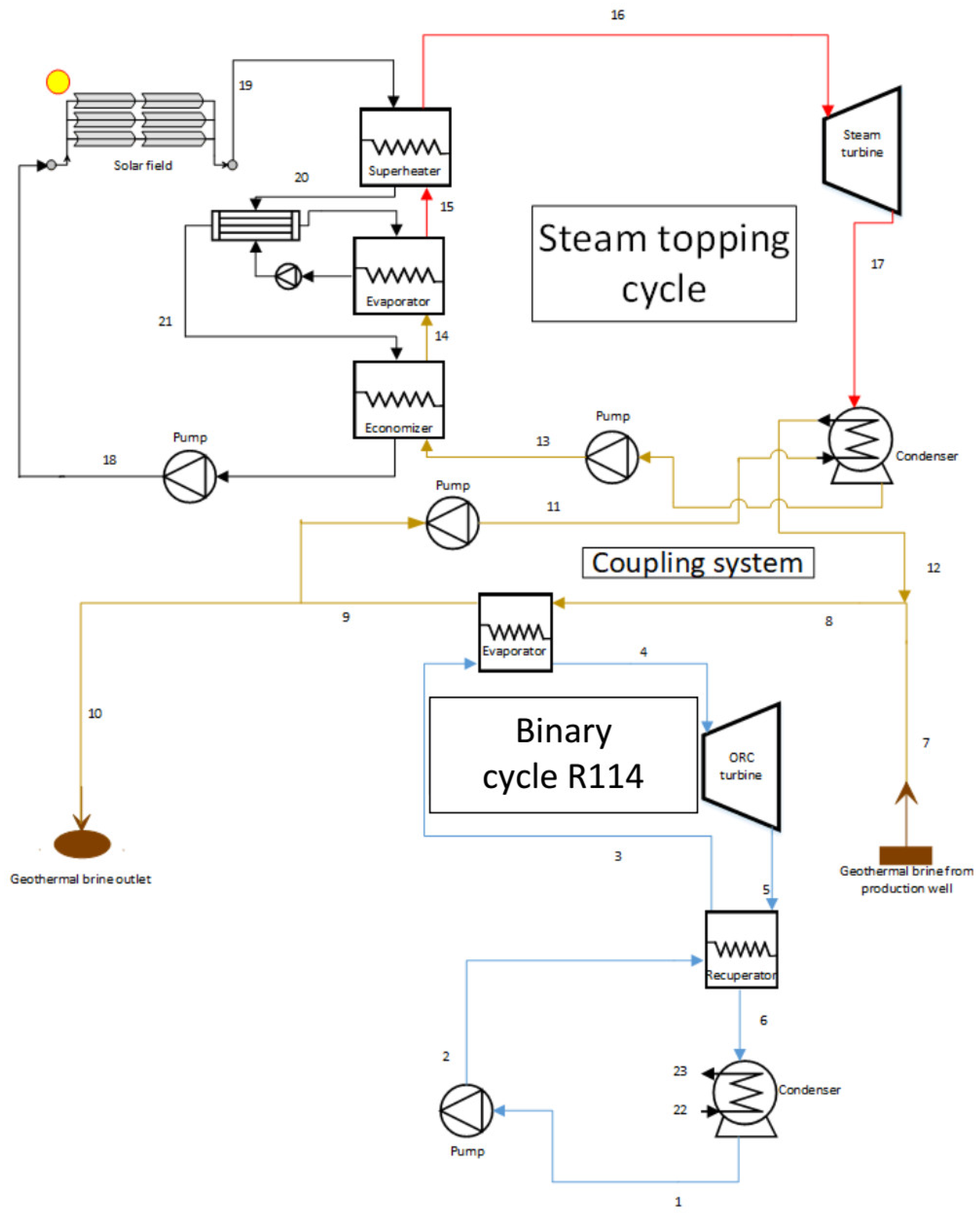
2.1. Project Approach

In this investigation, a hybrid geothermal–solar power plant was proposed to generate power to integrate the solar–steam ranking cycle with the geothermal section and the organic ranking cycle. Concentrating solar power (CSP) collectors can be used to produce heat that will supplement an underperforming geothermal plant. Increasing the turbine inlet mass flow rates and pressures by solar will then allow the geothermal turbines to operate closer to the design operating conditions, thereby increasing the efficiency and power production of the overall plant. In addition, thermal storage may be incorporated so that the added solar thermal energy can boost the power generation of the geothermal/solar hybrid plant independent of intermittent solar irradiance. Thermal storage enables energy from the hybrid plant to be time-shifted to periods in the day where utility market demand and energy rates are higher. Figure 1 represents the schematics of the hybrid geothermal–solar Rankin cycle.

2.1.1. Geothermal Source

The pressure and temperature of the boiler in geothermal source was supposed to be 10 bar and 150 °C, respectively, Bonyadi et al. [26], Başoğul [31], Zhou et al. [32]. A downstream heat exchanger was coupled to the source. The minimum temperature for releasing the salt was supposed to be 70 °C to reduce the construction of silica, Khalid et al. [33].

2.1.2. Downstream Cycle

R114 was selected as heat transfer fluid (HTF) for the ORC cycle. A heat exchanger gave the geothermal heat to fluid, and its temperature reached 150 °C. The turbine output was equipped with an improver to increase the efficiency of the downstream cycle, Alibaba et al. [34], Montazerinejad et al. [20].

2.1.3. The Solar Section in Upstream Cycle

The heat transfer fluid interface of the given power plant was a linear parabolic collector (LPC) with the lubricant oil. There was no thermal energy in the solar part of the storage enclosure and the temperature of collectors was 395 °C, Elmohlawy et al. [35], Ameri and Mohammadzadeh [36]. The fluid was circulated with controlled discharge using a pump in order to cause the fluid to reach the desired outlet temperature at the collector output. Additionally, some heat exchangers were applied to transfer the direct heat of the solar energy to the Rankine cycle. In this study, a solar power plant was designed so that thermal energy of the solar section was produced by 25% higher than the required amount, Baker et al. [37], Bonyadi et al. [26].

2.1.4. Ranking Steam Cycle in Upstream Cycle

As mentioned earlier, heat exchangers are used in three modes: economizers, evaporators and super heaters for the direct transfer of direct heat from the solar sector to the part of the Rankine cycle. The working fluid (water) enters the turbine after heat absorption and is finally poured into the converters through the pump after the heat dissipation in the condenser. Equipment used in this cycle is high-pressure equipment. Under the design conditions, the super heater steam enters a turbine at a constant temperature of 390 °C and leaves the turbine at 170 °C, Khalid et al. [33].

2.1.5. Creation of Thermal Coupling for Cycles

The geothermal power plant created heat and thermal coupling of the downstream and upstream and cycles. The low-temperature fluid of the geothermal cycle was addressed to the upstream condenser for reheating, and was blended with pure salt using a return cycle. The pump and flow controller adjusted the water temperature of the condenser of the solar cycle at 150 °C, Montazerinejad et al. [20].

2.2. Modes of Simulation

2.2.1. Standalone Geothermal State

In this case, only the downstream cycle was assumed to generate the power, and the solar field was considered uneconomical. The temperature and pressure of the water were 150 °C and 10 bar, respectively, Díaz et al. [7].

2.2.2. Hybrid Geothermal–Solar State

In this state, the geothermal section was able to produce a mass flow of 100 kg·s⁻¹. The solar module provided a flow rate of 100 kg·s⁻¹ during 12 hours a day. The mass flow rate was constant (at 100 kg·s⁻¹) during the day, and the heat source was 100% dependent on geothermal sources at night.

2.2.3. Conducting Simulation Using Software

To simulate the cycles, thermoflow software was used. The data required to simulate the organic part of the organic Rankine cycle were considered in accordance with the referenced article data, Bonyadi et al. [26]. Given that the geothermal section had different divergences in all models and that the solar and steam sections were added to the organic Rankine cycle by the geothermal section, we assumed that the input data for the organic Rankine section were the same for all models. These data are summarized in

Table 1. The design parameters of present study, Bonyadi et al. [26], Zhou et al. [30], Başoğul [31].

Parameters	Value
The flow rate of geothermal fluid (kg·s−1)	100
The pressure of the geothermal fluid (bar),	10
The temperature of the geothermal fluid (°C)	150
A minimum temperature of returned geothermal fluid (°C)	100
The temperature of inlet of turbine (°C)	130
Temperature of ambient (°C)	15
Efficiency of the turbine	0.85

. Also, the flowchart of modeling equations of system are given in Figure 2.

2.3. Thermodynamic Modeling

In order to calculate unknown temperatures, pressures and enthalpies of every state of the system, thermodynamic modeling was performed. This is the first step of any thermodynamic analysis to specify the system thermodynamically. Although this analysis is not capable of defining every aspect of the system, but since further analyses are based on thermodynamic modeling, it is a vital task to perform. Neccessary equations, theoretical analysis and input/output data for the component of the cycle are shown by

Table A3. Equations and theoretical analysis for Component of cycle.

Component	Relations	Inputs	Outputs
Solar collector	[${\mathrm{Q}}_{\mathrm{u}}$ = ${\mathrm{R}}_{\mathrm{f}}*{\mathrm{Q}}_{\mathrm{c}\mathrm{o}\mathrm{l}\mathrm{l}}$−${\mathrm{Q}}_{\mathrm{l}\mathrm{o}\mathrm{s}\mathrm{s},\mathrm{a}\mathrm{b}\mathrm{s}}$−${\mathrm{Q}}_{\mathrm{l}\mathrm{o}\mathrm{s}\mathrm{s},\mathrm{p}\mathrm{i}\mathrm{p}\mathrm{e}}$], [${\mathrm{Q}}_{\mathrm{u}}$ = ${\mathrm{m}}_{\mathrm{H}\mathrm{T}\mathrm{F}}$*(${\mathrm{h}}_{19}-{\mathrm{h}}_{18}$) [${\mathrm{Q}}_{\mathrm{c}\mathrm{o}\mathrm{l}\mathrm{l}}$ = $\mathrm{e}\mathrm{t}{\mathrm{a}}_{\mathrm{o}\mathrm{p}\mathrm{t}}$*${\mathrm{f}}_{\mathrm{s}\mathrm{h}\mathrm{a}\mathrm{d}}$*${\mathrm{M}}_{\mathrm{s}}$*${\mathrm{A}}_{\mathrm{c}\mathrm{o}\mathrm{l}\mathrm{l}}$*DNI], [${\mathrm{h}}_{19}$ = ${\mathrm{h}}_{@\mathrm{T}={\mathrm{T}}_{19},\mathrm{P}={\mathrm{P}}_{19}}$]	${\mathrm{h}}_{18}=890$, ${\mathrm{R}}_{\mathrm{f}}=1$, ${\mathrm{eta}}_{\mathrm{opt}}=0.741$, ${\mathrm{f}}_{\mathrm{shad}}=0.98$, ${\mathrm{M}}_{\mathrm{s}}=1.25$,${\mathrm{A}}_{\mathrm{coll}}=12225$, DNI =1000, ${\mathrm{m}}_{\mathrm{HTF}}=3.16$	${\mathrm{Q}}_{\mathrm{c}\mathrm{o}\mathrm{l}\mathrm{l}}$, ${\mathrm{Q}}_{\mathrm{l}\mathrm{o}\mathrm{s}\mathrm{s},\mathrm{a}\mathrm{b}\mathrm{s}}$ ${\mathrm{Q}}_{\mathrm{l}\mathrm{o}\mathrm{s}\mathrm{s},\mathrm{p}\mathrm{i}\mathrm{p}\mathrm{e}}$, ${\mathrm{Q}}_{\mathrm{u}} , {\mathrm{h}}_{19}$
Coupling Pump	[${\mathrm{W}}_{\mathrm{C}\mathrm{o}\mathrm{u}\mathrm{p}\mathrm{l}\mathrm{i}\mathrm{n}\mathrm{g} \mathrm{P}\mathrm{u}\mathrm{m}}$ = ${\mathrm{m}}_{11}$(${\mathrm{h}}_{11}-{\mathrm{h}}_9$)], [${\mathrm{P}}_{11}$ = ${\mathrm{P}}_{12}$/(1−$\mathrm{d}{\mathrm{p}}_{\mathrm{S}\mathrm{t}\mathrm{e}\mathrm{a}\mathrm{m} \mathrm{C}\mathrm{o}\mathrm{n}\mathrm{d}\mathrm{e}\mathrm{n}\mathrm{s}\mathrm{e}\mathrm{r}}$)] [${\mathrm{h}}_{11}$ = (${\mathrm{h}}_{11\mathrm{s}}-{\mathrm{h}}_9$)/ + ${\mathrm{h}}_9$]	${\mathrm{P}}_{12}=10$,${\mathrm{dp}}_{\mathrm{SCond}}=0.2$ ${\mathrm{eta}}_{\mathrm{CP}}=0.85$,${\mathrm{h}}_9=419.8 , {\mathrm{m}}_{11}$	${\mathrm{W}}_{\mathrm{Cp}}$, ${\mathrm{h}}_{11}$, ${\mathrm{P}}_{11}$
HTF Pump	[${\mathrm{W}}_{\mathrm{H}\mathrm{T}\mathrm{F} \mathrm{P}\mathrm{u}\mathrm{m}\mathrm{p}}$ = ${\mathrm{m}}_{\mathrm{H}\mathrm{T}\mathrm{F}}$(${\mathrm{h}}_{18}-{\mathrm{h}}_{24}$)], [${\mathrm{P}}_{18}$ = ${\mathrm{P}}_{19}$/(1−$\mathrm{d}{\mathrm{p}}_{\mathrm{S}\mathrm{o}\mathrm{l}\mathrm{a}\mathrm{r} \mathrm{F}\mathrm{i}\mathrm{e}\mathrm{l}\mathrm{d}}$)], [${\mathrm{h}}_{18}$ = (${\mathrm{h}}_{18\mathrm{s}}-{\mathrm{h}}_{24}$)/$\mathrm{e}\mathrm{t}{\mathrm{a}}_{\mathrm{H}\mathrm{T}\mathrm{F}\mathrm{P}}$ + ${\mathrm{h}}_{24}$]	${\mathrm{P}}_{19}=11.3$, ${\mathrm{dp}}_{\mathrm{Solar}\mathrm{Field}}=0.1$, ${\mathrm{eta}}_{\mathrm{HTFP}}=$${\mathrm{h}}_{24}=419$,${\mathrm{m}}_{\mathrm{HTF}}$ = 3.16	${\mathrm{W}}_{\mathrm{H}\mathrm{T}\mathrm{F}\mathrm{P}}$, ${\mathrm{h}}_{18}$, ${\mathrm{P}}_{18}$
ORC Condenser	[${\mathrm{m}}_{\mathrm{O}\mathrm{R}\mathrm{C} }$(${\mathrm{h}}_6-{\mathrm{h}}_1$) = ${\mathrm{m}}_{\mathrm{C}\mathrm{o}\mathrm{o}\mathrm{l} \mathrm{W}\mathrm{A}\mathrm{T}\mathrm{E}\mathrm{R}}$(${\mathrm{h}}_{23}-{\mathrm{h}}_{22}$)], [${\mathrm{T}}_{23}$ = ${\mathrm{T}}_{22}$ + $\mathrm{d}\mathrm{e}\mathrm{l}\mathrm{t}\mathrm{a}{\mathrm{T}}_{\mathrm{C}\mathrm{o}\mathrm{o}\mathrm{l} \mathrm{W}\mathrm{A}\mathrm{T}\mathrm{E}\mathrm{R}}$] [${\mathrm{P}}_{23}$ = ${\mathrm{P}}_{22}$(1−$\mathrm{d}\mathrm{e}\mathrm{l}\mathrm{t}\mathrm{a}{\mathrm{P}}_{\mathrm{C}\mathrm{o}\mathrm{o}\mathrm{l}\mathrm{i}\mathrm{n}\mathrm{g} \mathrm{W}\mathrm{A}\mathrm{T}\mathrm{E}\mathrm{R}}$)], [${\mathrm{h}}_1$ = ${\mathrm{h}}_{@\mathrm{x}=0,\mathrm{P}={\mathrm{P}}_{\mathrm{O}\mathrm{R}\mathrm{C}\mathrm{C}\mathrm{o}\mathrm{n}\mathrm{d}\mathrm{e}\mathrm{n}\mathrm{s}\mathrm{e}\mathrm{r}}}$], [${\mathrm{h}}_{22}$ = ${\mathrm{h}}_{@\mathrm{T}={\mathrm{T}}_{22},\mathrm{P}={\mathrm{P}}_{22}}$], [${\mathrm{h}}_{23}$ = ${\mathrm{h}}_{@\mathrm{T}={\mathrm{T}}_{23},\mathrm{P}={\mathrm{P}}_{23}}$]	${\mathrm{m}}_{\mathrm{ORC}}=135$,${\mathrm{h}}_6=369.4$,${\mathrm{h}}_{22}=63.07$,${\mathrm{h}}_1=235.3$, ${\mathrm{T}}_{22}=15$, ${\mathrm{P}}_{22}=1.01$,${\mathrm{deltaT}}_{\mathrm{CW}}=10$,${\mathrm{deltaP}}_{\mathrm{CW}}=0.02$, ${\mathrm{P}}_{\mathrm{ORCCond}}$ = 3	${\mathrm{h}}_1$, ${\mathrm{m}}_{\mathrm{C}\mathrm{W}}$ ${\mathrm{h}}_{23}$,${\mathrm{T}}_{23}$,${\mathrm{P}}_{23}$
ORC Evaporator	$[{\mathrm{m}}_{\mathrm{O}\mathrm{R}\mathrm{C} }$(${\mathrm{h}}_4-{\mathrm{h}}_3$) = ${\mathrm{m}}_{\mathrm{B}\mathrm{r}\mathrm{i}\mathrm{n}\mathrm{e}}$(${\mathrm{h}}_8-{\mathrm{h}}_9$)], [${\mathrm{m}}_{\mathrm{B}\mathrm{r}\mathrm{i}\mathrm{n}\mathrm{e}}$ = 100(kg/s)], $[{\mathrm{h}}_4$ = ${\mathrm{h}}_{@\mathrm{T}={\mathrm{T}}_4,\mathrm{P}={\mathrm{P}}_4}$], [${\mathrm{h}}_8$ = ${\mathrm{h}}_{@\mathrm{T}={\mathrm{T}}_8,\mathrm{P}={\mathrm{P}}_8}$], [${\mathrm{h}}_9$ = ${\mathrm{h}}_{@\mathrm{T}={\mathrm{T}}_9,\mathrm{P}={\mathrm{P}}_9}$]	${\mathrm{h}}_3=253.9$, ${\mathrm{h}}_4=410.8$, ${\mathrm{m}}_{\mathrm{Brine}}=100$	${\mathrm{m}}_{\mathrm{O}\mathrm{R}\mathrm{C} \mathrm{c}\mathrm{y}\mathrm{c}\mathrm{l}\mathrm{e}}$, ${\mathrm{h}}_8$,${\mathrm{h}}_9$
ORC Pump	$[{\mathrm{W}}_{\mathrm{O}\mathrm{R}\mathrm{C} \mathrm{P}\mathrm{u}\mathrm{m}\mathrm{p}}$ = ${\mathrm{m}}_{\mathrm{O}\mathrm{R}\mathrm{C}}$(${\mathrm{h}}_2-{\mathrm{h}}_1$)], $[{\mathrm{P}}_2$ = ${\mathrm{P}}_3$/(1−$\mathrm{d}{\mathrm{p}}_{\mathrm{O}\mathrm{R}\mathrm{C} \mathrm{R}\mathrm{e}\mathrm{c}\mathrm{u}\mathrm{p}\mathrm{e}\mathrm{r}\mathrm{a}\mathrm{t}\mathrm{o}\mathrm{r}}$)], [${\mathrm{h}}_2$ = (${\mathrm{h}}_{2\mathrm{s}}-{\mathrm{h}}_1$)/$\mathrm{e}\mathrm{t}{\mathrm{a}}_{\mathrm{O}\mathrm{R}\mathrm{C} \mathrm{P}\mathrm{u}\mathrm{m}\mathrm{p}}$ + ${\mathrm{h}}_1$]	${\mathrm{P}}_3=21.7$,${\mathrm{eta}}_{\mathrm{ORCP}}=0.8$,${\mathrm{h}}_1$=235.3	${\mathrm{W}}_{\mathrm{O}\mathrm{R}\mathrm{C} \mathrm{P}\mathrm{u}\mathrm{m}\mathrm{p}}$, ${\mathrm{h}}_2$,${\mathrm{P}}_2$
ORC Recuperator	$[{\mathrm{h}}_3-{\mathrm{h}}_2$ = ${\mathrm{h}}_5-{\mathrm{h}}_6$], [${\mathrm{P}}_6$ = ${\mathrm{P}}_{\mathrm{O}\mathrm{R}\mathrm{C}\mathrm{C}\mathrm{o}\mathrm{n}\mathrm{d}}$], [${\mathrm{P}}_3$ = ${\mathrm{P}}_4$/(1−$\mathrm{d}{\mathrm{p}}_{\mathrm{O}\mathrm{R}\mathrm{C}\mathrm{E}\mathrm{v}\mathrm{a}}$)]	${\mathrm{h}}_2=236.9$,${\mathrm{h}}_6=369.5$,${\mathrm{h}}_5=386.3$,${\mathrm{P}}_{\mathrm{ORCCon}}=3$,${\mathrm{dp}}_{\mathrm{ORCEva}}=0.03$,${\mathrm{P}}_2=21.9$	${\mathrm{h}}_3$, ${\mathrm{P}}_6$, ${\mathrm{P}}_3$
ORC Turbine	$[{\mathrm{W}}_{\mathrm{O}\mathrm{R}\mathrm{C}\mathrm{T}}$ = ${\mathrm{m}}_{\mathrm{O}\mathrm{R}\mathrm{C} }$(${\mathrm{h}}_4-{\mathrm{h}}_5$)], [${\mathrm{P}}_5$ = ${\mathrm{P}}_6$/(1−$\mathrm{d}{\mathrm{p}}_{\mathrm{O}\mathrm{R}\mathrm{C}\mathrm{R}\mathrm{e}\mathrm{c}}$)], [${\mathrm{h}}_5$ = ${\mathrm{h}}_4$−(${\mathrm{h}}_4-{\mathrm{h}}_{5\mathrm{s}}$) * $\mathrm{e}\mathrm{t}{\mathrm{a}}_{\mathrm{O}\mathrm{R}\mathrm{C}\mathrm{T}}$ ], [${\mathrm{P}}_6$ = ${\mathrm{P}}_{\mathrm{O}\mathrm{R}\mathrm{C}\mathrm{C}\mathrm{o}\mathrm{n}\mathrm{d}}$]	${\mathrm{m}}_{\mathrm{ORC}}=135.5$,${\mathrm{h}}_4=410.8$,${\mathrm{P}}_{\mathrm{ORCCon}}=0.1$ ${\mathrm{dp}}_{\mathrm{ORCRec}}=0.01$, ${\mathrm{eta}}_{\mathrm{ORCT}}=0.85$	${\mathrm{W}}_{\mathrm{O}\mathrm{R}\mathrm{C} \mathrm{T}\mathrm{u}\mathrm{r}\mathrm{b}\mathrm{i}\mathrm{n}\mathrm{e}}$, ${\mathrm{h}}_5$, ${\mathrm{P}}_5$
Steam Economizer	$[{\mathrm{m}}_{\mathrm{S}\mathrm{C}}$(${\mathrm{h}}_{14}-{\mathrm{h}}_{13}$) = ${\mathrm{m}}_{\mathrm{H}\mathrm{T}\mathrm{F}}$(${\mathrm{h}}_{21}-{\mathrm{h}}_{24}$)], [${\mathrm{h}}_{14}$ = ${\mathrm{h}}_{@\mathrm{x}={\mathrm{T}}_0,\mathrm{P}={\mathrm{P}}_{14}}$]	${\mathrm{m}}_{\mathrm{SC}}$,${\mathrm{h}}_{13}=691.07$, ${\mathrm{m}}_{\mathrm{HTF}}=3.16$,${\mathrm{h}}_{21}=955.8$	${\mathrm{h}}_{14}$, ${\mathrm{h}}_{24}$
Steam Pump	$[{\mathrm{W}}_{\mathrm{S}\mathrm{t}\mathrm{e}\mathrm{a}\mathrm{m} \mathrm{P}\mathrm{u}\mathrm{m}\mathrm{p}}$ = ${\mathrm{m}}_{\mathrm{S}\mathrm{C}}$(${\mathrm{h}}_{13}-{\mathrm{h}}_{25}$)], [${\mathrm{P}}_{13}$ = ${\mathrm{P}}_{14}$/(1−$\mathrm{d}{\mathrm{p}}_{\mathrm{E}\mathrm{c}\mathrm{o}\mathrm{n}\mathrm{o}\mathrm{m}\mathrm{i}\mathrm{z}\mathrm{e}\mathrm{r}}$)], [${\mathrm{h}}_{13}$ = (${\mathrm{h}}_{13\mathrm{s}}-{\mathrm{h}}_{25}$)/$\mathrm{e}\mathrm{t}{\mathrm{a}}_{\mathrm{S}\mathrm{P}}$ + ${\mathrm{h}}_{25}$]	${\mathrm{P}}_{14}=60.2$,${\mathrm{dp}}_{\mathrm{Eco}}=0.2$,${\mathrm{eta}}_{\mathrm{sp}}=0.85$, ${\mathrm{h}}_{25}=684.08$,${\mathrm{m}}_{\mathrm{SC}}$	${\mathrm{W}}_{\mathrm{S}\mathrm{P}}$, ${\mathrm{h}}_{13}$, ${\mathrm{P}}_{13}$
Steam Super heater	$[{\mathrm{m}}_{\mathrm{S}\mathrm{C}}$(${\mathrm{h}}_{16}-{\mathrm{h}}_{15}$) = ${\mathrm{m}}_{\mathrm{H}\mathrm{T}\mathrm{F}}$(${\mathrm{h}}_{19}-{\mathrm{h}}_{20}$)], [${\mathrm{h}}_{16}$ = ${\mathrm{h}}_{@\mathrm{T}={\mathrm{T}}_{16},\mathrm{P}={\mathrm{P}}_{16}}$]	${\mathrm{m}}_{\mathrm{SC}}$, ${\mathrm{h}}_{15}=2784.4$, ${\mathrm{m}}_{\mathrm{HTF}}=3.16$, ${\mathrm{h}}_{19}=1222.4$	${\mathrm{h}}_{16}$, ${\mathrm{h}}_{20}$
Steam Turbine	$[{\mathrm{W}}_{\mathrm{S}\mathrm{t}\mathrm{e}\mathrm{a}\mathrm{m} \mathrm{T}}$ = ${\mathrm{m}}_{\mathrm{S}\mathrm{C}}$(${\mathrm{h}}_{16}-{\mathrm{h}}_{17}$)], [${\mathrm{h}}_{17}$ = ${\mathrm{h}}_{16}$−(${\mathrm{h}}_{16}-{\mathrm{h}}_{17\mathrm{s}}$) * $\mathrm{e}\mathrm{t}{\mathrm{a}}_{\mathrm{S}\mathrm{t}\mathrm{e}\mathrm{a}\mathrm{m} \mathrm{T}}$ ], $[{\mathrm{P}}_{17}$ = ${\mathrm{P}}_{\mathrm{S}\mathrm{t}\mathrm{e}\mathrm{m}\mathrm{C}\mathrm{o}\mathrm{n}\mathrm{d}\mathrm{e}\mathrm{n}\mathrm{s}\mathrm{e}\mathrm{r}}$ ]	${\mathrm{m}}_{\mathrm{SC}}$, ${\mathrm{h}}_{16}=3152.4$, ${\mathrm{eta}}_{\mathrm{S}\mathrm{T}}=0.87$,${\mathrm{P}}_{\mathrm{SCond}}=6.5$	${\mathrm{W}}_{\mathrm{S}\mathrm{t}\mathrm{e}\mathrm{a}\mathrm{m} \mathrm{T}}$, ${\mathrm{h}}_{17}$, ${\mathrm{P}}_{17}$
Steam Condenser	$[ {\mathrm{m}}_{\mathrm{S}\mathrm{T} \mathrm{C}\mathrm{o}\mathrm{n}\mathrm{d}}$(${\mathrm{h}}_{17 }$- ${\mathrm{h}}_{25}$) = ${\mathrm{m}}_{11}$(${\mathrm{h}}_{12}-{\mathrm{h}}_{11}$)], [${\mathrm{T}}_{12}$ = 150 (C)],$[{\mathrm{P}}_{12}$=10(bar)] $[{\mathrm{h}}_{25}$ = ${\mathrm{h}}_{@\mathrm{x}=0,\mathrm{P}={\mathrm{P}}_{\mathrm{S}\mathrm{t}\mathrm{e}\mathrm{a}\mathrm{m}\mathrm{C}\mathrm{o}\mathrm{n}\mathrm{d}}}$], [${\mathrm{h}}_{12}$ = ${\mathrm{h}}_{@\mathrm{T}={\mathrm{T}}_{12},\mathrm{P}={\mathrm{P}}_{12}}$]	${\mathrm{m}}_{\mathrm{SC}}$,${\mathrm{h}}_{17}=2724.5$,${\mathrm{h}}_{11}=419.86$, ${\mathrm{T}}_{12}=150$,${\mathrm{P}}_{12}=10$,${\mathrm{P}}_{\mathrm{S}\mathrm{Cond}}=6.5$	${\mathrm{h}}_{25}$, ${\mathrm{h}}_{12}$, ${\mathrm{m}}_{11}$
Steam Evaporator	$[ {\mathrm{m}}_{\mathrm{S}\mathrm{T} \mathrm{E}\mathrm{v}\mathrm{a}}$(${\mathrm{h}}_{15}-{\mathrm{h}}_{14}$) = ${\mathrm{m}}_{\mathrm{H}\mathrm{T}\mathrm{F}}$(${\mathrm{h}}_{20}-{\mathrm{h}}_{21}$)], [${\mathrm{h}}_{15}$ = ${\mathrm{h}}_{@\mathrm{x}=1,\mathrm{P}={\mathrm{P}}_{15}}$], [${\mathrm{h}}_{21}$ = ${\mathrm{h}}_{15}$ + $\mathrm{\Delta }{\mathrm{T}}_{\mathrm{P}\mathrm{i}\mathrm{n}\mathrm{c}\mathrm{h}}$]	${\mathrm{h}}_{14}=1189.2$, ${\mathrm{m}}_{\mathrm{HTF}}=3.16$, ${\mathrm{h}}_{20}=1172.4$	${\mathrm{h}}_{15}$, ${\mathrm{h}}_{21}$,${\mathrm{m}}_{\mathrm{S}\mathrm{C}}$

of Appendix A.

First, the thermodynamic modeling was performed by Thermoflow software which is an industrial instrument with a significantly real and effective data bank related to power cycle components. Next, the first law of thermodynamic analysis was carried out by programming in Matlab software.

Mass and energy balances are fundamental equations of 1st law analysis. These balances can be written for each component according to mass (Equation (1)) and material (Equation (2)) and energy (Equation (3)) balances.

$${\displaystyle \sum }\dot{m}=0$$

(1)

$${\displaystyle \sum }\dot{mx}=0$$

(2)

$${\displaystyle \sum }\dot{Q}+{\displaystyle \sum }\dot{W}+{\displaystyle \sum }\dot{m}h =0$$

(3)

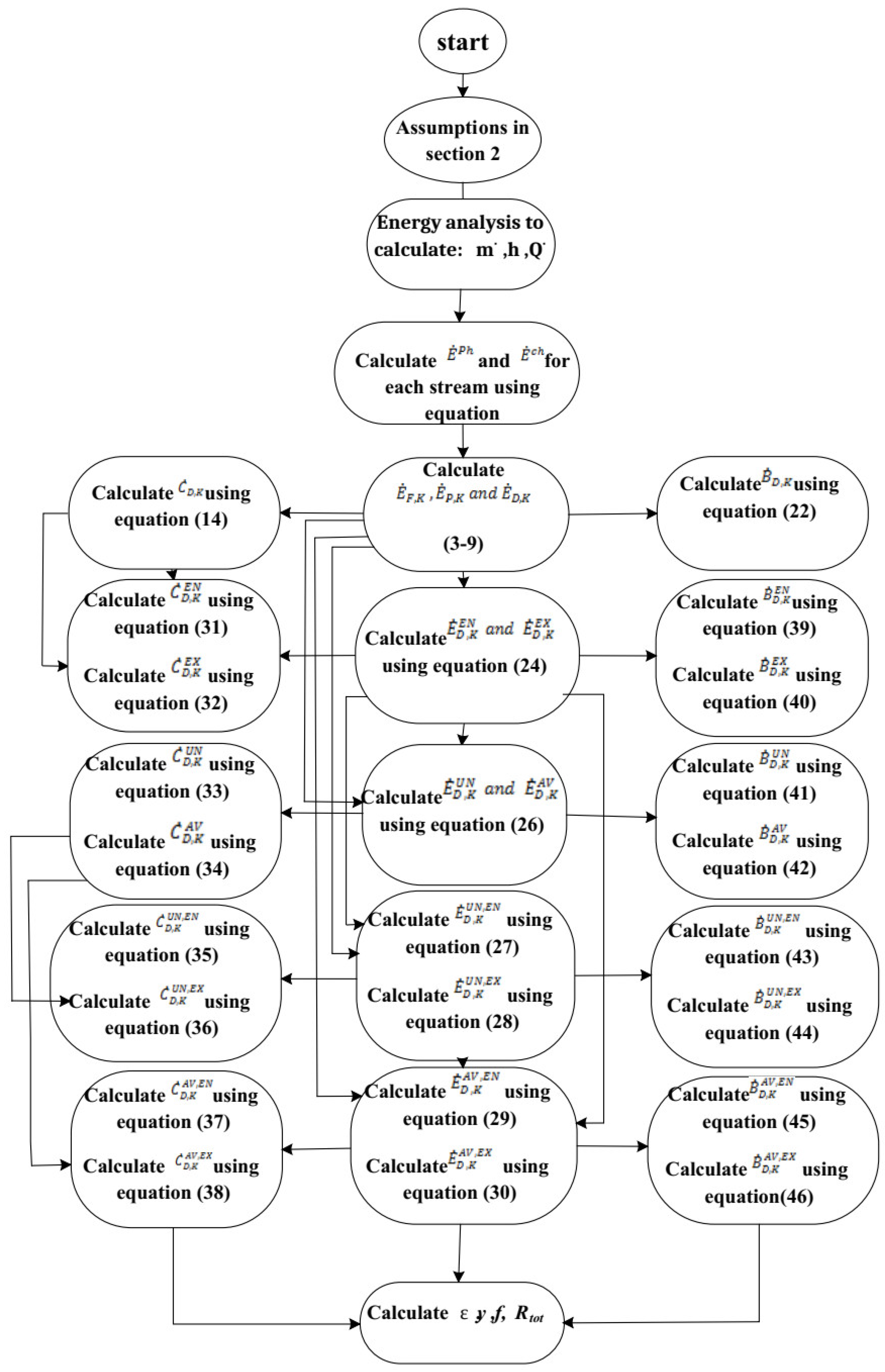
2.4. Exergy Analysis

An exergy analysis, which is based on the second law of thermodynamics, can be performed to determine the thermodynamic irreversibility in the components. Exergy rates are generally composed of four elements: physical (${\dot{E}}^{ph}$), chemical (${\dot{E}}^{ch}$), kinetic (${\dot{E}}^{ke}=\frac{1}{2}\dot{m}{V}^2$) and potential (${\dot{E}}^{pe}=\dot{m}gz$). Specific exergy can be given as, Yunus et al. [39], Almutairi et al. [40].

$$\dot{E}={\dot{E}}^{\mathit{ph}}+{\dot{E}}^{\mathit{ch}}+{\dot{E}}^{\mathit{pe}}+{\dot{E}}^{\mathit{ke}}$$

(4)

The formula for calculating the physical exergy rate is as follows, Yu et al. [38]:

$${\dot{E}}^{\mathit{ph}}=\dot{m}\left[\left({\mathrm{h}}_{\mathrm{i}}-{\mathrm{h}}_{\mathrm{o}}\right)-{\mathrm{T}}_{\mathrm{O}}\left({\mathrm{s}}_{\mathrm{i}}-{\mathrm{s}}_{\mathrm{o}}\right)\right].$$

(5)

The formula for calculating the chemical exergy rate is expressed as follows, Yu et al. [38]:

$${\dot{E}}^{ch}=\dot{m}\left[{{\displaystyle \sum }}_{i=1}^n{x}_i{e}_{0,i}^{ch}+R{T}_0{{\displaystyle \sum }}_{i=1}^n{x}_i\mathit{ln}\left(x_i\right)\right]$$

(6)

where (n) represents the number of moles of the component in the inorganic matter, in mol.kg-1. $e_{0,i}^{ch}$ and $x_i$ are the standard chemical exergy and mole fraction of components(i) in inorganic matter, respectively. R is the universal gas constant, 0.0083145 kJ. (mol.K)⁻¹, Eboh et al. [41].

One of the most important concepts of exergy analysis is calculating the fuel and the product streams for each component. Every component needs a driver to continue working which is defined as the fuel stream of the equipment and every component has an output and goal to produce which is the product stream of that component.

See Equation (7) for the specific flow rates of exergy. After calculating fuel and product of the equipment, Ochoa et al. [42], further outputs of exergy analysis, i.e., exergy destruction (${\dot{E}}_D$) and exergetic efficiency (${\psi }_k$) of each component can be determined from Equations (8) and (9).

$${\dot{E}}_k={\dot{ m}}_k·e_k$$

(7)

$${\dot{E}}_D={\dot{E}}_F-{\dot{E}}_P={\displaystyle \sum }{\dot{E}}_{in}-{\displaystyle \sum }{\dot{E}}_{out}+{\displaystyle \sum }\dot{Q}\left(1-\frac{T_0}{T}\right)+{\displaystyle \sum }\dot{W}$$

(8)

$${\psi }_{k }=\frac{{\dot{E}}_{P,k}}{{\dot{E}}_{F,k}}$$

(9)

where $e_k$ is the specific exergy of the streams, ${\dot{E}}_{in}$ and ${\dot{E}}_{out}$ are the exergy of heat input and work output. The ${\dot{E}}_{P,k}$ and ${\dot{E}}_{F,k}$ are the exergy rates associated with the product and fuel of each component, Ochoa et al. [43]. The definition of input–output is applied to a traditional exergetic analysis, where the input is the amount of exergy that enters a component to produce an amount of product. Similarly, the product exergy is defined as the amount of exergy left by a component converted by the fuel exergy that previously entered the same component. For the specific case of the component under study k, the exergy rate of fuel (${\dot{E}}_F)$, product (${\dot{E}}_p)$ and destruction (${\dot{E}}_D)$ is given by Equation (8). The exergetic efficiency (${\psi }_k$) of each component can be determined from Equation (9).

2.5. Exergo-Economic Analysis

Economic issues as an inevitable part of engineering were considered in a thermodynamic so-called exergo-economic analysis. Price estimates, assumptions and calculated values for the equipment cost rate are shown in Appendix A, which shows the cost functions for all components.

* See

Table 2. Equations related to the exergo-economic analysis.

Definition	Equation
The equipment cost rate, Heberle et al. [44].	${\dot{Z}}_k=\frac{{\Phi }_k·PE{C}_k·CRF}{3600·N}$	(10)
The Capital Recovery Factor, Heberle et al. [44].	$CRF=\frac{{(1+i)}^n.i}{(\left(1+i{)}^n\right)-1}$	(11)
The cost rate of the streams, Montazerinejad et al. [20].	${\dot{C}}_i=c_i·{\dot{E}}_i$	(12)
The exergo-economic balance for each component, Montazerinejad et al. [20].	${\dot{C}}_{P,k}={\dot{C}}_{F,k}-{\dot{C}}_{L,k}+{\dot{Z}}_k$	(13)
The cost rate of exergy destruction of equipment, Carotenuto et al. [45].	${\dot{C}}_{D,k}=c_{F,k}·{\dot{E}}_{D,k}$	(14)
The exergo-economic factor, Montazerinejad et al. [20].	$f_K=\frac{{\dot{Z}}_k}{{\dot{Z}}_k+c_{f,k}·{\dot{E}}_{D,k}}$	(15)
The relative cost difference of the equipment indicates, Montazerinejad et al. [20]	$r_K=\frac{c_{P,k}-c_{F,k}}{c_{F,k}}=\frac{1-{\psi }_k}{{\psi }_k}$ + $\frac{{\dot{Z}}_k}{c_{f,k}·{\dot{E}}_{P,k}}$	(16)

for the equations needed for the exergo-economic analysis.

Equation (6) determines the cost rate of equipment that $PE{C}_k$ is the amortization cost for a particular component and ${\Phi }_k$ is a maintenance coefficient and determines the impact of maintenance costs on total cost of equipment that is assumed (1.06). The number of system operating hours in a year for power plant (N) is considered (8100) for the ORC cycle and (4380) for the topping cycle. The (Capital Recovery Factor) CRF estimated (0.0825) by Equation (11) where (i) is the interest rate and (n) is the number of lifetime years considered as 30 years.

For calculating the cost per exergy unit, the exergo-economic balance of each component should be obtained according to Equations (12) and (13) where $c_i$ is the cost of the streams, ${\dot{C}}_P$ is the cost rate of the equipment, ${\dot{C}}_F$ is the cost rate of fuel flow and ${\dot{Z}}_k$ is the cost rate dependent on the maintenance cost and capital cost rate of each component.

2.6. Exergo-Environmental Analysis

Considering the impact of power production systems on the environment is essential, Appendix A gives the weight; environmental impact of material and calculated values for the environmental impact of all components.

See

Table 3. Equations needed for the exergo-environmental analysis.

Definition	Equation
The relationship between environmental impact and exergy for each stream, Cardemil et al. [46].	${\dot{B}}_i=b_i·{\dot{E}}_i$	(17)
The exergy environmental balances of equipment, Cardemil et al. [46].	${\displaystyle \sum }{\dot{B}}_{in,k}-{\displaystyle \sum }{\dot{B}}_{out,k}+{\dot{Y}}_k=0$	(18)
The environmental impact of the equipment, Cardemil et al. [46].	${\dot{Y}}_k=\frac{Y_k}{3600·t·n}$	(19)
The exergy environmental impact of the fuel streams of the equipment, pts.kJ-1, Açıkkalp et al. [47].	$b_{F,k}=\frac{{\dot{B}}_{F,k}}{{\dot{E}}_{F,k}}$	(20)
The exergy environmental impact of the product streams of the equipment, pts.kJ-1, Açıkkalp et al. [47].	$b_{P,k}=\frac{{\dot{B}}_{P,k}}{{\dot{E}}_{P,k}}$	(21)
The environmental rate of exergy destruction of equipment, Díaz, et al. [7].	${\dot{B}}_{D,k}=b_{F,k}·{\dot{E}}_{D,k}$	(22)
The exergo environmental factor, Díaz et al. [7].	$f{b}_{K }=\frac{{\dot{Y}}_k}{{\dot{Y}}_k+b_{f,k}·{\dot{E}}_{D,k}}$	(23)

for equations of the exergo-environmental analysis.

Here, ${\dot{B}}_i$ is the environmental exergy rate in (pts.s-1),$b_i$ is the exergy-environmental impact in (pts.kJ-1) and $\dot{E}$ is the exergy rate of i^th flow in kW; ${\dot{Y}}_k$ is the environmental destruction rate of component k in (pts.s-1), and it can be determined by ecological indicators 99 (ECO), Cavalcanti [48].

In order to determine $Y_k$, the weight of each component and its environmental impact per weight unit should be used in tons and mpts.kJ-1, respectively.

2.7. Advanced Exergy Analysis

The main idea is that the equipment irreversibility is not only due to the weak thermodynamic performance of the equipment itself, but also to the performance of other equipment associated with it, Akbari and Sheikhi [2].

In this analysis, equipment irreversibility is divided into two categories: one from perspective of the origin of irreversibility and the other from the perspective of the ability to eliminate irreversibility. The irreversibility of each device is categorized into endogenous irreversibility and exogenous irreversibility.

Endogenous irreversibility is the part of irreversibility that is related to the intrinsic performance of the equipment itself and the type of energy conversion process that occurs in it, and even if other equipment operates in its ideal condition and is not irreversible, this part is irreversible. Exogenous irreversibility is also part of the irreversibility, which is the inductive effect of irreversibility on other devices.

The irreversible division is of importance, and obtained results indicate the quality of the layout and structure of the process; however, performing it and calculating the endogenous irreversibility of the equipment is more complex. In fact, it is a major issue of advanced exergy analysis. In this regard, first, a hybrid cycle was designed in which all components, except the studied component, operated under a theoretical state. The endogenous irreversibility of the component was obtained by calculating its energy degradation in this cycle.

Unavoidable irreversibility is a part of irreversibility that is not eliminated due to technical and economic constraints and will always exist, and avoidable irreversibility is part of irreversibility that can be solved with little cost and modification of the equipment. Determination of the unavoidable irreversibility depends on the technical and economic constraints of process design, and the hypothetical criteria are provided by the analyst himself. The input values of main parameters used in the simulation are listed in

Table 4. The input values of the main parameters in the advanced exergy analysis.

Component	Isentropic Efficiency	Component	Pinch Point (°C)
Coupling Pump	0.85	ORC Condenser	9.54
HTF Pump	0.85	ORC Evaporator	6.8
ORC Pump	0.80	ORC Recuperator	2
ORC Turbine	0.85	Steam Economiser	15
Steam Pump	0.85	Steam Evaporator	10
Steam Turbine	0.87	Steam Superheater	5
		Topping Condenser	12.5

, Javanshir et al. [49], Darvish et al. [50], Matuszewska et al. [51], Wei et al. [52], Dibazar et al. [53].

It is not enough to have only information about exogenous/endogenous and avoidable/unavoidable irreversibility to evaluate the performance of the equipment, but there is also a need for more information in this regard. Therefore, the total exergy destruction was categorized into endogenous-avoidable exergy destruction, endogenous-unavoidable exergy destruction, exogenous-avoidable exergy destruction and exogenous-unavoidable exergy destruction, as can be seen in

Table 5. Equations for the advanced exergy analysis.

Definition	Equation
The relationship between exogenous and endogenous and irreversibility for each component, Akbari et al. [2], Wang et al. [22].Cavalcanti [48],	${\dot{E}}_{D.K }^{EX}={\dot{E}}_{D.K}-{\dot{E}}_{D.K}^{EN}$	(24)
The relationship between Avoidable and Unavoidable Irreversibility for each stream, Wang et al. [22], Sert and Balkan [23], Voloshchuk [54].	${\dot{E}}_{D.K}={\dot{E}}_{D.K}^{AV}+{\dot{E}}_{D.K}^{UN}$	(25)
Unavoidable exergy destruction rate of a component, Ochoa et al. [43].	${\dot{E}}_{D.K}^{UN}={\dot{E}}_{P.K}{\left(\frac{{\dot{E}}_D}{{\dot{E}}_P}\right)}_K^{UN}$	(26)
Unavoidable endogenous exergy destruction rate of a component, Tsatsaronis and Morosuk [55].	${\dot{E}}_{D.K}^{UN.EN}={\dot{E}}_{P.K}^{EN}{\left(\frac{{\dot{E}}_D}{{\dot{E}}_P}\right)}_K^{UN}=E_{F,K}^{UN}{\left(\frac{{\dot{E}}_D}{{\dot{E}}_P}\right)}^{EN}$	(27)
Unavoidable exogenous exergy destruction rate of a component, Wang et al. [22].	${\dot{E}}_{D.K}^{UN.EX}={\dot{E}}_{D.K}^{UN}-{\dot{E}}_{D.K}^{UN.EN}$	(28)
Avoidable endogenous exergy destruction rate of a component, Ochoa et al. [42,43].	${\dot{E}}_{D.K}^{AV.EN}={\dot{E}}_{D.K}^{EN}-{\dot{E}}_{D.K}^{UN.EN}$	(29)
Avoidable exogenous exergy destruction rate of a component, Tsatsaronis and Morosuk [55].	${\dot{E}}_{D.K}^{AV.EX}={\dot{E}}_{D.K}^{AV}-{\dot{E}}_{D.K}^{AV.EN}$	(30)

.

2.8. Advanced Exergoeconomic Analysis

An advanced exergo-economic analysis is used as a useful tool for calculating and comparing the exergy destruction of equipment. Similarly, for determining the economic interaction between components of system, exergy destruction and its costs were divided into endogenous/erogenous and unavoidable/unavoidable sectors, respectively. Results of advanced exergo-economic analysis of the proposed system are shown in

Table 6. Equations for the advanced exergo-economic analysis of the proposed system.

Definition of Cost Rate	Equations
The cost of the kth component that is called the endogenous cost, Islam and Dincer [9]	${\dot{C}}_{D,K}^{EN}=c_{F,K}{\dot{E}}_{D,K}^{EN}$	(31)
The exogenous cost of kth component, Ochoa et al. [43]	${\dot{C}}_{D,K}^{EX}={\dot{C}}_{D,K}-{\dot{C}}_{D,K}^{EN}$	(32)
Unavoidable cost of exergy destruction, Ochoa et al. [43]	${\dot{C}}_{D,K}^{UN}=c_{F,K}{\dot{E}}_{D,K}^{UN}$	(33)
Avoidable cost rate, Cavalcanti [48]	${\dot{C}}_{D,K}^{\mathit{AV}}=c_{F,K}{\dot{E}}_{D,K}^{\mathit{AV}}$	(34)
Unavoidable cost rate of kth component associated with the operation of the component itself, Ochoa et al. [43]	${\dot{C}}_{D,K}^{UN,EN}=c_{F,K}{\dot{E}}_{D,K}^{UN,EN}$	(35)
Unavoidable cost rate of kth component caused by the remaining components, Islam and Dincer [9]	${\dot{C}}_{D,K}^{UN,EX}={\dot{C}}_{D,K}^{UN}-{\dot{E}}_{D,K}^{UN,EN}$	(36)
Avoidable cost rate of kth component associated with the operation of the component itself, Ochoa et al. [43]	${\dot{C}}_{D,K}^{\mathit{AV},EN}={\dot{C}}_{D,K}^{EN}-{\dot{E}}_{D,K}^{UN,EN}$	(37)
Avoidable cost rate of kth component caused by the remaining components, Ochoa et al. [43]	${\dot{C}}_{D,K}^{\mathit{AV},EX}={\dot{C}}_{D,K}^{EX}-{\dot{E}}_{D,K}^{UN,EX}$	(38)

.

2.9. Advanced Exergo-Environmental Analysis

Advanced exergo-economic analysis separates effective environmental components and exergy destruction into unavoidable/avoidable and endogenous/exogenous parts and compounds them in different possible modes, Yürüsoy and Keçebaş [56].

The environmental impact of the exogenous exergy destruction rate (${\dot{B}}_{D,K}^{EX}$) was affiliated with the relations between the components, while the environmental impact of the endogenous exergy destruction rate (${\dot{B}}_{D,K}^{EN}$) was affiliated with irreversible environmental impacts of the component itself. Moreover, the environmental impact of exergy destruction rate was categorized into unavoidable (${\dot{B}}_{D,K}^{UN}$) and avoidable (${\dot{B}}_{D,K}^{\mathit{AV}}$) parts. Categorizing the environmental impact of exergy destruction into improvable and un-improvable sections was assumed as well. The four parts of the environmental impact of the exergy destruction rate were avoidable endogenous environmental impact of the exergy destruction rate (${\dot{B}}_{D,K}^{\mathit{AV},EN}$), unavoidable endogenous environmental impact of the exergy destruction rate (${\dot{B}}_{D,K}^{UN,EN}$), avoidable exogenous environmental impact of the exergy destruction rate (${\dot{B}}_{D,K}^{\mathit{AV},EX}$) and unavoidable exogenous environmental impact of the exergy destruction rate (${\dot{B}}_{D,K}^{UN,EX}$), Tsatsaronis and Morosuk [55]. See

Table 7. Equations for the advanced exergo-environmental analysis of the proposed system, Cheng et al. [21], Ochoa et al. [43].

Description	Equations
Endogenous exergy destruction rate	${\dot{B}}_{D,K}^{EN}=b_{F,K}{\dot{E}}_{D,K}^{EN}$	(39)
Exogenous exergy destruction rate	${\dot{B}}_{D,K}^{EX}=b_{F,K}{\dot{E}}_{D,K}^{EX}$	(40)
Unavoidable exergy destruction rate	${\dot{B}}_{D,K}^{UN}=b_{F,K}{\dot{E}}_{D,K}^{UN}$	(41)
Avoidable exergy destruction rate	${\dot{B}}_{D,K}^{\mathit{AV}}=b_{F,K}{\dot{E}}_{D,K}^{\mathit{AV}}$	(42)
Unavoidable endogenous exergy destruction rate	${\dot{B}}_{D,K}^{UN,EN}=b_{F,K}{\dot{E}}_{D,K}^{UN,EN}$	(43)
Unavoidable exogenous exergy destruction rate	${\dot{B}}_{D,K}^{UN,EX}=b_{F,K}{\dot{E}}_{D,K}^{UN,EX}$	(44)
Avoidable endogenous exergy destruction rate	${\dot{B}}_{D,K}^{\mathit{AV},EN}=b_{F,K}{\dot{E}}_{D,K}^{\mathit{AV},EN}$	(45)
Avoidable exogenous exergy destruction rate	${\dot{B}}_{D,K}^{\mathit{AV},EX}=b_{F,K}{\dot{E}}_{D,K}^{\mathit{AV},EX}$	(46)

for all equations correlated to the advanced exergo-environmental analysis.

3. Results

The results of the thermodynamic analysis showed that the net production of the cycle with working fluids of R114 and R123 was 4172 and 4129 kW, respectively. The thermal efficiency of the hybrid cycle with R114 and R123 was 14.40% and 14.25%, respectively, while the use of R134a generated power of 5923 kW and efficiency of 14.55%. Another important point is that the amount of energy received from the geothermal source for the R114, R123 and R134a were 21,266, 21,266 and 32,734 kW, respectively. This indicated that although R134a had a higher production capacity, its efficiency was equal to the other two working fluids. Moreover, it received more energy from the geothermal source.

Exergetic evaluation of system showed that the exergetic efficiency of the drive cycle with fluids of R114 and R123 was 24.15% and 23.90%, respectively, which decreased by 6.08% and 6.33% compared to R134a. As a result, it was observed that the use of R134a performed better from a thermodynamic point of view.

Exergo-conomic evaluation of the system showed that the total cost of the hybrid power plant for R134a, R114 and R123 (including the cost of equipment and currents flowing into the power plant) was USD.s-1 0.0508, 0.0444 and 0.0426, respectively. Although R134a was more productive, it imposed more costs.

An assessment of the given cycle from an exergo-environmental perspective based on life cycle assessment (LCA) showed that R134a had more adverse effects on the environment than the other two fluids. Thus, the environmental impact with this fluid was 6.22e-5 (Pts.s-1), which was 9.51% higher than the environmental impact of R114 and 10.28% higher than the adverse environmental impact of R123. Therefore, the use of R134a, in addition to costing more, will also have more environmental degradation. Thus, R114 was selected as the working fluid for the present paper.

Table 8. Flow information of first and second modes of simulation.

State	Standalone Geothermal Cycle (GPP)					Second Mode (Hybrid Geothermal-Solar)
	$\dot{\mathit{m}}$ kg·s−1	T (°C)	P (bar)	h (kJ·kg−1)	${\mathit{E}}_{\mathit{x}}$ (kw)	$\dot{\mathit{m}}$ kg·s−1	T (°C)	P (bar)	h (kJ·kg−1)	${\mathit{E}}_{\mathit{x}}$ (kw)
1	135.5	35.9	3	235.3	866.4	135.5	35.9	3	235.3	866.4
2	135.5	37.12	21.9 56.2	236.9	1049.4	135.5	37.12	21.9	236.9	1049.4
3	135.5	53.76	21.6	253.9	1266.4	135.5	53.76	21.7	253.9	1266.4
4	135.5	130	21.03	410.9	6282.7	135.5	130	21	410.9	6282.7
5	135.5	72.58	3.06	386.4	2476.6	135.5	72.58	3.1	386.4	2476.6
6	135.5	50	3	369.5	2123.9	135.5	50	3	369.5	2123.9
7	100	150	10	632.5	7219	-	-	-	632.5	7219
8	100	150	10	632.5	10355	100	150	10	632.5	10355
9	100	100	10	419.8	4496.9	100	100	10	419.8	4496.9
10	-	-	-	-	-	69.71	100	10	419.8	3134.9
11	-	-	-	-	-	30.3	100.002	10.2	419.9	1362.6
12	-	-	-	-	-	30.3	150	10	632.5	3136.4
13	-	-	-	-	-	3.156	162.87	60.41	691.1	399.4
14	-	-	-	-	-	3.156	270.8	60.21	1189.2	1046.1
15	-	-	-	-	-	3.156	275.8	60.21	2784.4	3437.9
16	-	-	-	-	-	3.156	390	60	3152.4	4039.3
17	-	-	-	-	-	3.156	162	6.5	2724.5	2554.9
18	-	-	-	-	-	23.2	256.1	12.4	890.2	5489
19	-	-	-	-	-	23.2	395	11.3	1222.40	1053.6
20	-	-	-	-	-	23.2	375.9	11.2	1172.5	9750.6
21	-	-	-	-	-	23.2	285.8	11.1	955.8	6440.2
22	434.4	15	1.013	63.08	0	434.4	15	1.013	63.08	0
23	434.4	25	0.996	104.9	307.3	434.4	25	0.993	104.9	307.3

gives information of temperature, mass flow, enthalpy, pressure and exergy rate in GPP and SGPP cycles.

Considering a conventional exergy analysis using the equations for each component of the cycles presented in

Table 9. Exergo-economic analysis results of the standalone geothermal cycle (GPP).

Component	$\dot{\mathit{E}}{\mathit{x}}_{\mathit{D}}$ (kW)	$\dot{\mathit{E}}{\mathit{x}}_{\mathit{F}}$ (kW)	$\dot{\mathit{E}}{\mathit{x}}_{\mathit{P}}$ (kW)	${\mathit{\psi }}_{\mathit{k}}$ (%)	$\dot{\mathit{Z}}$ (USD.S−1)	${\dot{\mathit{C}}}_{\mathit{F}}$ (USD.S−1)	${\dot{\mathit{C}}}_{\mathit{P}}$ (USD.S−1)	${\dot{\mathit{C}}}_{\mathit{D}}$ (USD.S−1)	r	F (%)
ORC Condenser	950.1578	-	-	-	7.21E-04	-	-	-	-	-
ORC Evaporator	842.2208	5.86E+03	5.02E+03	85.62	3.11E-04	0.0103	0.0106	1.50E-03	0.2033	17.42
ORC Pump	59.9911	242.9772	182.9861	75.31	5.25E-04	0.0014	0.0019	3.36E-04	0.8399	60.97
ORC Recuperator	135.6746	352.7151	217.0405	61.53	2.76E-05	0.0012	0.0013	4.70E-04	0.6617	5.554
ORC Turbine	491.5625	3.81E+03	3.31E+03	87.09	0.005364067	0.0132	0.0186	0.0017	0.615	75.89

and

Table 10. The results of exergo-economic analysis of each component in the solar–geothermal cycle (SGPP).

Component	$\dot{\mathit{E}}{\mathit{x}}_{\mathit{D}}$ (kW)	$\dot{\mathit{E}}{\mathit{x}}_{\mathit{F}}$ (kW)	$\dot{\mathit{E}}{\mathit{x}}_{\mathit{P}}$ (kW)	${\mathit{\psi }}_{\mathit{k}}$ (%)	$\dot{\mathit{Z}}$ (USD.S−1)	${\dot{\mathit{C}}}_{\mathit{F}}$ (USD.S−1)	${\dot{\mathit{C}}}_{\mathit{P}}$ (USD.S−1)	${\dot{\mathit{C}}}_{\mathit{D}}$ (USD.S−1)	r	f (%)
Coupling Pump	8.6E-02	7.4E-01	6.57E-01	88.42	2.20E-06	1.52E-05	1.74E-05	1.76E-06	2.95E-01	0.00E+00
HTF Pump	2.0E+00	5.1E+00	3.09E+00	60.52	6.24E-05	1.04E-04	1.66E-04	4.11E-05	1.64E+00	0.00E+00
ORC Condenser	9.5E+02	-	-	-	7.21E-04	-	-	-	-	-
ORC Evaporator	8.4E+02	5.9E+03	5.02E+03	85.62	5.14E-04	1.03E-02	1.08E-02	1.47E-03	2.26E-01	1.74E+01
ORC Pump	6.0E+01	2.4E+02	1.83E+02	75.31	5.25E-04	1.40E-03	1.90E-03	3.40E-04	8.34E-01	6.10E+01
ORC Recuperator	1.4E+02	3.5E+02	2.17E+02	61.53	3.02E-05	1.20E-03	1.30E-03	4.78E-04	6.65E-01	5.55E+00
ORC Turbine	4.9E+02	3.8E+03	3.31E+03	87.08	5.36E-03	1.34E-02	1.88E-02	1.70E-03	6.07E-01	7.59E+01
SolarField(Collector)	6.4E+03	1.1E+04	5.05E+03	44.21	2.41E-02	0.00E+00	2.41E-02	0.00E+00	-	1.00E+02
Steam Economizer	3.1E+02	9.5E+02	6.47E+02	67.76	3.26E-04	4.58E-03	4.91E-03	1.48E-03	5.81E-01	1.81E+01
Steam Evaporator	9.2E+02	3.3E+03	2.39E+03	72.25	7.79E-04	1.59E-02	1.67E-02	4.41E-03	4.52E-01	1.50E+01
Steam Pump	2.2E+00	2.2E+01	1.99E+01	90.08	2.13E-05	4.50E-04	4.72E-04	4.47E-05	1.63E-01	3.23E+01
Steam Super heater	1.8E+02	7.9E+02	6.01E+02	76.57	2.59E-04	3.77E-03	4.03E-03	8.84E-04	3.96E-01	2.27E+01
Steam Turbine	1.3E+02	1.5E+03	1.35E+03	91	3.31E-03	2.42E-02	2.76E-02	2.18E-03	2.49E-01	6.03E+01
Topping Condenser	4.0E+02	-	-	-	1.29E-03	-	-	-	-	-

, the exergy destruction rates were obtained.

The main results of the conventional exergy analysis for GPP and SGPP are presented in Table 9 and Table 10, respectively. $\dot{\mathit{E}}{\mathit{x}}_{\mathit{F}} , \dot{\mathit{E}}{\mathit{x}}_{\mathit{P}},\dot{\mathit{E}}{\mathit{x}}_{\mathit{D}} ,{\mathit{\psi }}_{\mathit{k}}$ in these tables are exergy of fuel, exergy of product, exergy destruction and exergetic efficiency, Dibazar et al. [53]. It can be said that the components with higher exergy destruction rates had more effects on the efficiency of systems from an exergy point of view compared with other components. Referring to Table 9, in the GPP cycle, the maximum exergy destruction rate happened in the ORC condenser, followed by the ORC evaporator and the ORC turbine. Table 10 shows the exergy destruction rates for the SGPP cycle components; the maximum exergy destruction rate happened in the solar field, followed by the orc condenser and the steam evaporator. The solar implemented power plant had a higher rate of exergy destruction. This is because of the higher temperature difference between hot and cold streams, Mohammadi et al. [57].

Additionally, the rate of exergy destruction can be decreased if one could reduce the inlet temperature of the hot fluid in shell and tube heat exchangers provided that the required heat transfer rate is supplied, Mehrpooya et al. [58]. As a summary, it can be concluded that the solar field, ORC condenser and ORC evaporator have more potential to reduce their destructive rates and to increase system efficiency, Bonyadi et al. [26].

In addition, the results obtained from the traditional exergo-economic analysis are shown in Table 9 and Table 10. The greater the investment $(\dot{\mathit{Z}}$) and the cost of exergy destroyed $\left({\dot{\mathit{C}}}_{\mathit{D}}\right)$, the greater the influence of the component in the system, therefore, the component with the greatest improvement in cost efficiency of the total plant could be defined, Ochoa et al. [43].

The exergo-economic factor, r, is the effective parameter that allows one to compare and evaluate the components that make up the system. A high value for this parameter indicated that for the component under study, acquisition costs predominated over operation and maintenance costs. For example, in the case of the condenser, which was the component with the lowest value of the exergo-economic factor, it can be concluded that expenses were mostly related to operating and maintenance costs compared to acquisition costs. The results of the exergo-economic analysis associated with the GPP cycle of simulation determined that the maximum investment cost in the cycle was related to the ORC condenser. Additionally, the maximum cost of exergy destruction was associated with the ORC turbine.

The results of the exergo-economic analysis of the SGPP cycle showed that the solar power plant had the maximum investment cost. The maximum cost of exergy destruction was the evaporator.

The exergo-environmental results for the GPP and SGPP cycles are given in

Table 11. Exergo-environmental results for standalone geothermal cycle (GPP).

Component	$\dot{\mathit{Y}}$ (pts.S−1)	${\mathit{b}}_{\mathit{F}}$ (pts.kJ−1)	${\mathit{b}}_{\mathit{P}}$ (pts.kJ−1)	${\mathit{B}}_{\mathit{F}}$ (pts.kJ−1)	${\mathit{B}}_{\mathit{P}}$ (pts.kJ−1)	${\mathit{B}}_{\mathit{D}}$ (pts.kJ−1)	${\mathit{r}}_{\mathit{b}}$	${\mathit{f}}_{\mathit{b}}$ (%)
OCR Condenser	4.13E-08	-	-	-	-	-	-	-
OCR Evaporator	3.56E-06	0.00E+00	7.10E-10	0.00E+00	3.56E-06	0.00E+00	Inf	100.0
OCR Pump	2.27E-08	4.04E-09	5.50E-09	9.83E-07	1.01E-06	2.43E-07	0.36	8.6
OCR Recuperator	1.22E-07	1.24E-09	2.58E-09	4.38E-07	5.61E-07	1.69E-07	1.08	42.1
OCR Turbine	8.68E-06	1.24E-09	4.04E-09	4.73E-06	1.34E-05	6.11E-07	2.26	93.4

and

Table 12. Exergo-environmental calculations in the solar–geothermal cycle (SGPP).

Component	$\dot{\mathit{Y}}$ (pts.S−1)	${\mathit{b}}_{\mathit{F}}$ (pts.kJ−1)	${\mathit{b}}_{\mathit{P}}$ (pts.kJ−1)	${\mathit{B}}_{\mathit{F}}$ (pts.kJ−1)	${\mathit{B}}_{\mathit{P}}$ (pts.kJ−1)	${\mathit{B}}_{\mathit{D}}$ (pts.kJ−1)	${\mathit{r}}_{\mathit{b}}$	${\mathit{f}}_{\mathit{b}}$ (%)
Coupling Pump	1.29E-09	3.36E-08	3.99E-08	2.49E-08	2.62E-08	2.89E-09	0.19	30.9
HTF Pump	8.05E-09	3.36E-08	5.81E-08	1.71E-07	1.79E-07	6.75E-08	0.73	10.7
ORC Condenser	4.13E-08	-	-	-	-	-	-	-
ORC Evaporator	3.56E-06	0	7.10E-10	0	3.56E-06	0	Inf	100.0
ORC Pump	2.27E-08	4.04E-09	5.50E-09	9.83E-07	1.01E-06	2.43E-07	0.36	8.6
ORC Recuperator	1.22E-07	1.24E-09	2.58E-09	4.38E-07	5.61E-07	1.69E-07	1.08	42.1
ORC Turbine	8.68E-06	1.24E-09	4.04E-09	4.73E-06	1.34E-05	6.11E-07	2.26	93.4
Solar Field(Collector)	2.03E-05	0.00E+00	4.03E-09	0.00E+00	2.03E-05	0.00E+00	-	100.0
Steam Economizer	2.33E-07	4.06E-09	6.36E-09	3.88E-06	4.11E-06	1.25E-06	0.56	15.7
Steam Evaporator	2.47E-06	4.06E-09	6.66E-09	1.34E-05	1.59E-05	3.73E-06	0.64	39.8
Steam Pump	3.24E-08	3.36E-08	3.89E-08	7.41E-07	7.73E-07	7.35E-08	0.16	30.6
Steam Super heater	1.29E-05	4.06E-09	2.68E-08	3.19E-06	1.61E-05	7.48E-07	5.60	94.5
Steam Turbine	8.33E-06	2.49E-08	3.36E-08	3.70E-05	4.53E-05	3.33E-06	0.35	71.4
Topping Condenser	2.73E-08	-	-	-	-	-	-	-

, respectively. According to Table 11, the turbine had the highest environmental impact on the equipment, and the highest exergy destruction. After that, the evaporator had the highest environmental impact but its exergy destruction was zero. In the second mode, the solar panel had the highest environmental impact of the equipment, but due to environmental impacts of fuel flow of the solar panel, exergy destruction was zero.

According to Table 12, in the SGPP cycle, the solar panel had the highest environmental impact of the equipment, but due to environmental impacts of fuel flow of the solar panel, exergy destruction was zero, because the environmental impacts of fuel flow of the solar panel was zero. The steam evaporator in the geothermal solar cycle had the highest impact on environmental exergy degradation, Açıkkalp et al. [47], Cavalcanti [48].

As a summary, it can be concluded that solar field, orc condenser, evaporators and turbine have more potential to reduce their destructive rates and to increase system efficiency. As is seen, a conventional exergy analysis only focuses on components with high rates of exergy destruction, and it is not possible to specify whether these destructions occur in other components or in the component itself. This irreversibility may only be specified by advanced exergy tools. As discussed above, an advanced exergy analysis evaluates the effects of component interactions and the real possibility of components to improve system efficiency.

By advanced exergy analysis, the exergy destructions of each component calculated in the previous section can be discussed in detail to find the sources of these destructions and the real potentials of each component to amend the efficiency of the whole system. As mentioned above, these irreversibilities can be divided into exogenous, endogenous, unavoidable and avoidable parts to help researchers observe the effects of technological limitations and component interactions on the exergetic efficiency of a system for improvements, Morosuk and Tsatsaronis [16]. In the advanced exergy analysis, the endogenous part of exergy loss for the kth component was calculated by defining real and ideal conditions for the cycles first. Then, the exogenous destruction rate was obtained by the difference of the total exergy and endogenous part (Equation (24)). To calculate the unavoidable exergy rate of loss in the kth part, instead of real conditions in cycles, unavoidable conditions were considered, and avoidable exergy was obtained from Equation (25). Furthermore, the values of exogenous/avoidable, endogenous/avoidable, exogenous/unavoidable and endogenous/unavoidable were determined using Equations (26) to (30). Advanced exergy analysis results for each part in three different cycles (GPP, and SGPP) are presented in

Table 13. The results of advanced exergy analysis of the standalone geothermal cycle (GPP).

Component	${\dot{\mathit{E}}}_{\mathit{D}.\mathit{K}}$ (kW)	${\dot{\mathit{E}}}_{\mathit{D}.\mathit{K}}^{\mathit{E}\mathit{N}}$ (kW)	${\dot{\mathit{E}}}_{\mathit{D}.\mathit{K}}^{\mathit{E}\mathit{X}}$ (kW)	${\dot{\mathit{E}}}_{\mathit{D}.\mathit{K}}^{\mathit{A}\mathit{V}}$ (kW)	${\dot{\mathit{E}}}_{\mathit{D}.\mathit{K}}^{\mathit{U}\mathit{N}}$ (kW)	${\dot{\mathit{E}}}_{\mathit{D}.\mathit{K}}^{\mathit{E}\mathit{N},\mathit{A}\mathit{V}}$ (kW)	${\dot{\mathit{E}}}_{\mathit{D}.\mathit{K}}^{\mathit{E}\mathit{N},\mathit{U}\mathit{N}}$ (kW)	${\dot{\mathit{E}}}_{\mathit{D}.\mathit{K}}^{\mathit{E}\mathit{X},\mathit{A}\mathit{V}}$ (kW)	${\dot{\mathit{E}}}_{\mathit{D}.\mathit{K}}^{\mathit{E}\mathit{X},\mathit{U}\mathit{N}}$ (kW)	F (%)
ORC Condenser	950.16	758.70	191.46	282.01	668.15	225.18	533.52	56.82	134.63	-
ORC Evaporator	842.22	693.23	148.99	124.23	717.99	102.25	590.98	21.98	127.01	91.67
ORC Pump	59.99	53.64	6.35	9.08	50.91	8.12	45.52	0.96	5.39	74.92
ORC Recuperator	135.67	108.85	26.82	11.29	124.39	9.06	99.80	2.23	24.59	66.45
ORC Turbine	491.56	424.32	67.25	47.09	444.47	40.65	383.67	6.44	60.80	84.44

and

Table 14. Advanced exergy analysis of each component in the solar–geothermal cycle (SGPP).

Component	${\dot{\mathit{E}}}_{\mathit{D}.\mathit{K}}$ (kW)	${\dot{\mathit{E}}}_{\mathit{D}.\mathit{K}}^{\mathit{E}\mathit{N}}$ (kW)	${\dot{\mathit{E}}}_{\mathit{D}.\mathit{K}}^{\mathit{E}\mathit{X}}$ (kW)	${\dot{\mathit{E}}}_{\mathit{D}.\mathit{K}}^{\mathit{A}\mathit{V}}$ (kW)	${\dot{\mathit{E}}}_{\mathit{D}.\mathit{K}}^{\mathit{U}\mathit{N}}$ (kW)	${\dot{\mathit{E}}}_{\mathit{D}.\mathit{K}}^{\mathit{E}\mathit{N},\mathit{A}\mathit{V}}$ (kW)	${\dot{\mathit{E}}}_{\mathit{D}.\mathit{K}}^{\mathit{E}\mathit{N},\mathit{U}\mathit{N}}$ (kW)	${\dot{\mathit{E}}}_{\mathit{D}.\mathit{K}}^{\mathit{E}\mathit{X},\mathit{A}\mathit{V}}$ (kW)	${\dot{\mathit{E}}}_{\mathit{D}.\mathit{K}}^{\mathit{E}\mathit{X},\mathit{U}\mathit{N}}$ (kW)	F (%)
Coupling Pump	0.09	0.07	0.01	0.01	0.08	0.01	0.07	0.00	1.14E-02	87.48
HTF Pump	2.01	1.82	0.20	0.21	1.81	0.19	1.63	0.02	1.76E-01	81.5
ORC Condenser	950.16	810.10	140.05	97.20	852.96	82.87	727.23	14.33	1.26E+02	-
ORC Evaporator	842.22	759.26	82.96	71.42	770.80	64.39	694.88	7.03	7.59E+01	92.25
ORC Pump	59.99	47.33	12.66	8.55	51.44	6.75	40.58	1.81	1.09E+01	74.92
ORC Recuperator	135.67	105.23	30.45	29.41	106.26	22.81	82.42	6.60	2.38E+01	70.7
ORC Turbine	491.56	428.79	62.77	66.66	424.91	58.14	370.65	8.51	5.43E+01	84.41
Solar Field(Collector)	6368.10	4408.64	1959.46	2514.13	3853.97	1740.53	2668.11	773.60	1.19E+03	44.14
Steam Economizer	307.68	222.64	85.04	99.97	207.72	72.34	150.30	27.63	5.74E+01	68.01
Steam Evaporator	918.56	648.41	270.15	258.67	659.89	182.59	465.82	76.07	1.94E+02	72.03
Steam Pump	2.19	1.98	0.21	0.21	1.98	0.19	1.79	0.02	1.94E-01	90.26
Steam Super heater	184.07	136.69	47.38	42.81	141.25	31.79	104.90	11.02	3.64E+01	75.03
Steam Turbine	133.66	121.93	11.72	10.89	122.76	9.94	112.00	0.96	1.08E+01	91.14
Topping Condenser	401.66	350.37	51.29	58.48	343.18	51.01	299.36	7.47	4.38E+01	-

.

As indicated in Table 13, for the GPP cycle, the endogenous exergy rate was greater than the exogenous exergy rate in system components. The greater share of exergy destruction in the ORC condenser was caused by the irreversibility of the component itself because of its high exergy loss rate in the endogenous part. As previously discussed, the avoidable destruction rate in exergy can be controlled and reduced in practice. Table 13 shows that an ORC condenser consists of a high value of avoidable destruction rates (282.01 kW) among the components of a system. Thus, the efficiency of this component can be improved using some technical modifications and new technologies or by replacing the component with those with higher efficiencies. It is important to note that, unlike the conventional analysis, an ORC condenser is the most effective component due to its avoidable destruction rate to reduce irreversibilities. So, the main focus was on the avoidable/endogenous parts of the exergy destruction, which can be decreased by improving the efficiency of the kth component. This was followed by an investigation on the exogenous/avoidable exergy rates of loss, which can be reduced by improving the efficiency of other parts, Tsatsaronis and Morosuk [59]. As it is stated in Galindo et al. [60], Table 13 shows that the avoidable/endogenous exergy destruction rates in the ORC condenser were greater than the unavoidable/endogenous destruction rates for the GPP cycle. This shows that the efficiency can be improved by technical modifications of this component. Table 13 also indicates that the exogenous/unavoidable exergy destruction rates were higher than the exogenous/avoidable exergy rates of loss for the components, Dibazar et al. [53].

In Table 14, for the SGPP cycle, the endogenous exergy destruction rate was higher than the exogenous exergy destruction rate in the system’s components, which showed that the greater share of the destruction rate was because of the internal irreversibility in the component itself. So, among all components in the SGPP cycle, the solar field consisted of the highest destruction rate in the exogenous part (1959.46 kW), and also had the maximum endogenous destruction rate (4408.64 kW) among the system’s components due to its irreversibility.

As seen in Table 14, the unavoidable part of the exergy destruction rate was higher than the avoidable part in all components of the SGPP cycle. This indicated that there was a low potential in the system to reduce its irreversibilities by using some efficient and new components. Splitting the exergy destruction rates into endogenous/avoidable and exogenous/avoidable parts provides some important information that helps researchers to optimize systems. As seen in Table 14, the avoidable/endogenous exergy destruction rates in most of the equipment were higher than the exogenous/avoidable rates. Priority in the improvement process of a component should be given to the solar field, the Steam Evaporator and the ORC condenser because of their higher values in the endogenous/avoidable destruction rates, Ochoa et al. [43], Dibazar et al. [53].

Equations (31)–(38) were used to calculate the advance exergy destruction costs as shown in

Table 15. Advanced exergo-economic analysis for the standalone geothermal cycle (GPP).

Component	${\dot{\mathit{C}}}_{\mathit{D}.\mathit{K}}$ (USD.S−1)	${\dot{\mathit{C}}}_{\mathit{D}.\mathit{K}}^{\mathit{E}\mathit{N}}$ (USD.S−1)	${\dot{\mathit{C}}}_{\mathit{D}.\mathit{K}}^{\mathit{E}\mathit{X}}$ (USD.S−1)	${\mathit{C}}_{\mathit{D}.\mathit{K}}^{\mathit{A}\mathit{V}}$ (USD.S−1)	${\dot{\mathit{C}}}_{\mathit{D}.\mathit{K}}^{\mathit{U}\mathit{N}}$ (USD.S−1)	${\dot{\mathit{C}}}_{\mathit{D}.\mathit{K}}^{\mathit{E}\mathit{N},\mathit{A}\mathit{V}}$ (USD.S−1)	${\dot{\mathit{C}}}_{\mathit{D}.\mathit{K}}^{\mathit{E}\mathit{N},\mathit{U}\mathit{N}}$ (USD.S−1)	${\dot{\mathit{C}}}_{\mathit{D}.\mathit{K}}^{\mathit{E}\mathit{X},\mathit{A}\mathit{V}}$ (USD.S−1)	${\dot{\mathit{C}}}_{\mathit{D}.\mathit{K}}^{\mathit{E}\mathit{X},\mathit{U}\mathit{N}}$ (USD.S−1)	F (%)
ORC Condenser	-	-		-	-	-	-	-	-	-
ORC Evaporator	0.0012	1.34E-03	1.60E-04	2.87E-04	1.21E-03	2.56E-04	1.08E-03	3.06E-05	1.30E-04	91.67
ORC Pump	-	3.00E-04	3.56E-05	5.82E-05	2.78E-04	5.20E-05	2.48E-04	6.16E-06	2.94E-05	74.92
ORC Recuperator	4.43E-04	3.98E-04	7.22E-05	4.81E-05	4.22E-04	4.07E-05	3.58E-04	7.37E-06	6.48E-05	66.45
ORC Turbine	0.0032	1.52E-03	1.81E-04	1.95E-04	1.51E-03	1.74E-04	1.35E-03	2.07E-05	1.60E-04	84.44

, which was based on the result of the advanced destroyed exergy. It can be observed that the endogenous exergy destruction was higher than the exogenous cost in the components of the GPP cycle. Therefore, it can be established that the interaction between component costs is not very relevant in the system; however, for the component under study, it was a parameter of vital importance. Additionally, it can be observed that the rates of unavoidable costs for the components studied showed an inclination in the unavoidable part.

In Table 15, the highest endogenous exergy destruction cost was due to the ORC turbine (1.52E-03 USD.S⁻¹), followed by the ORC evaporator (1.34E-03 USD.S⁻¹), ORC pump (3.98E-04 USD.S⁻¹) and ORC pump (3.00E-04 USD.S⁻¹), respectively, which indicated that the exergy destruction cost rates of these components were reduced. It was clearly observed that the values of $C_{D.K}^{AV}$ in the ORC evaporator and ORC turbine were higher than those in other components which signified the improvement potentials of these components, while the unavoidable part of the exergy destruction cost rates of the ORC turbine and ORC evaporator were in high level.

The economic improvement potential of the elements was determined by the evaluation of their avoidable/endogenous exergy destruction cost rates. In Table 15, the highest value of ${\dot{C}}_{\mathrm{D}.\mathrm{K}}^{EN,AV}$ was of the ORC evaporator (2.56E-04 USD.S⁻¹), followed by the ORC turbine (1.74E-04E USD.S⁻¹) and the ORC pump (5.20E-05 USD.S⁻¹). This fact implies that by improving these components, the system exergy destruction cost rate can be reduced significantly and the components must be considered themselves, instead of other components. It should be noticed that the values of ${\dot{C}}_{\mathrm{D}.\mathrm{K}}^{EX}$ in the ORC turbine (1.81E-04 USD.S⁻¹) and the ORC evaporator (1.60E-04 USD.S⁻¹) were higher, demonstrating that if the performance of the remaining components rises, the exergy destruction cost rate of these components will decrease. The ORC evaporator had the highest value of ${\dot{C}}_{\mathrm{D}.\mathrm{K}}^{EN,AV}$ (2.56E-04 USD.S⁻¹), and we can reduce the sizable portion of its exergy destruction cost by improving the exergy efficiency of the other component. Additionally, ${\dot{C}}_{D.K}^{EX,AV}$ in the ORC evaporator was huge in comparison with the other components, associated with the exergy destruction cost rate of the other components.

In

Table 16. Advanced exergo-economic analysis for hybrid solar–geothermal cycle (SGPP).

Component	${\dot{\mathit{C}}}_{\mathit{D}.\mathit{K}}$ (USD.S−1)	${\dot{\mathit{C}}}_{\mathit{D}.\mathit{K}}^{\mathit{E}\mathit{N}}$ (USD.S−1)	${\dot{\mathit{C}}}_{\mathit{D}.\mathit{K}}^{\mathit{E}\mathit{X}}$ (USD.S−1)	${\mathit{C}}_{\mathit{D}.\mathit{K}}^{\mathit{A}\mathit{V}}$ (USD.S−1)	${\dot{\mathit{C}}}_{\mathit{D}.\mathit{K}}^{\mathit{U}\mathit{N}}$ (USD.S−1)	${\dot{\mathit{C}}}_{\mathit{D}.\mathit{K}}^{\mathit{E}\mathit{N},\mathit{A}\mathit{V}}$ (USD.S−1)	${\dot{\mathit{C}}}_{\mathit{D}.\mathit{K}}^{\mathit{E}\mathit{N},\mathit{U}\mathit{N}}$ (USD.S−1)	${\dot{\mathit{C}}}_{\mathit{D}.\mathit{K}}^{\mathit{E}\mathit{X},\mathit{A}\mathit{V}}$ (USD.S−1)	${\dot{\mathit{C}}}_{\mathit{D}.\mathit{K}}^{\mathit{E}\mathit{X},\mathit{U}\mathit{N}}$ (USD.S−1)	F (%)
Coupling Pump	1.18E-06	6.73E-07	5.03E-07	1.45E-07	1.03E-06	8.31E-08	5.89E-07	4.28E+01	4.41E-07	87.48
HTF Pump	9.51E-06	8.57E-06	9.40E-07	1.19E-06	8.33E-06	1.07E-06	7.50E-06	9.88E+00	8.23E-07	81.5
ORC Condenser	-	-	-	-	-	-	-	-	-	-
ORC Evaporator	0.0011	1.02E-03	8.40E-05	1.06E-04	9.94E-04	9.82E-05	9.18E-04	7.64E+00	7.59E-05	92.25
ORC Pump	9.86E-04	7.42E-04	2.43E-04	1.83E-04	8.03E-04	1.38E-04	6.05E-04	2.47E+01	1.98E-04	74.92
ORC Recuperator	3.93E-04	2.92E-04	1.01E-04	1.04E-04	2.89E-04	7.70E-05	2.15E-04	2.56E+01	7.42E-05	70.7
ORC Turbine	0.0033	2.95E-03	3.54E-04	7.06E-04	2.59E-03	6.30E-04	2.32E-03	1.07E+01	2.79E-04	84.41
Solar Field(Collector)	0	0.00E+00	0.00E+00	0.00E+00	0.00E+00	0.00E+00	0.00E+00	3.58E+01	0.00E+00	44.14
Steam Economizer	0.0014	1.10E-03	3.03E-04	5.38E-04	8.62E-04	4.22E-04	6.75E-04	2.16E+01	1.86E-04	68.01
Steam Evaporator	0.0045	3.26E-03	1.24E-03	1.41E-03	3.09E-03	1.02E-03	2.24E-03	2.76E+01	8.55E-04	72.03
Steam Pump	4.72E-05	4.31E-05	4.14E-06	5.88E-06	4.14E-05	5.37E-06	3.77E-05	8.77E+00	3.63E-06	90.26
Steam Super heater	9.64E-04	7.06E-04	2.58E-04	2.84E-04	6.80E-04	2.08E-04	4.98E-04	2.67E+01	1.82E-04	75.03
Steam Turbine	2.20E-03	1.99E-03	2.12E-04	3.80E-04	1.82E-03	3.43E-04	1.65E-03	9.64E+00	1.75E-04	91.14
Topping Condenser	-	-	-	-	-	-	-	-	-	-

, the highest endogenous exergy destruction cost was due to the steam evaporator (3.26E-03 USD.S⁻¹), followed by the ORC turbine (2.95E-03 USD.S⁻¹), the steam turbine (1.99E-03 USD.S⁻¹) and the steam economizer (1.10E-03 USD.S⁻¹), respectively, which indicated that the exergy destruction cost rates of these components were reduced. It was clearly observed that the values of $C_{D.K}^{AV}$ in the steam evaporator and ORC turbine were higher than those in the other components which signified the improvement potentials of these components, while the unavoidable part of exergy destruction cost rates of the steam evaporator and ORC turbine were of a high level, Boyaghchi and Sabaghian [24].

The economic improvement potential of elements was determined by the evaluation of their avoidable/endogenous exergy destruction cost rates. In Table 16, the highest value of ${\dot{C}}_{\mathrm{D}.\mathrm{K}}^{EN,AV}$ was of the steam evaporator (1.02E-03 USD.S⁻¹), followed by the ORC turbine (6.30E-04 USD.S⁻¹) and the steam economizer (4.22E-04 USD.S⁻¹). This fact implies that by improving these components, the system exergy destruction cost rate can be reduced significantly and the components must be considered themselves, instead of other components. It should be noticed that the values of ${\dot{C}}_{\mathrm{D}.\mathrm{K}}^{EX}$ in the steam evaporator (3.03E-04 USD.S⁻¹) and the ORC turbine (3.54E-04 USD.S⁻¹) were higher, demonstrating that if the performance of the remaining components rises, the exergy destruction cost rate of these components will decrease. The steam evaporator had the highest value of ${\dot{C}}_{\mathrm{D}.\mathrm{K}}^{EN,AV}$ (1.02E-03 USD.S⁻¹) and we can reduce the sizable portion of its exergy destruction cost by improving exergy efficiency of the other component. Additionally, ${\dot{C}}_{D.K}^{EX,AV}$ in the Coupling Pump was huge (4.28E+01 USD.S⁻¹) in comparison with the other components, associated with the exergy destruction cost rate of other components. With regard to the auxiliary heater, the results showed that the amount of ${\dot{C}}_{D.K}^{EN}$ in the solar field was around zero because the exergy destruction cost rate of auxiliary heater is dependent on other components and only half of ${\dot{C}}_{D.K}^{Ex}$ can be avoided by using new technologies in other components.

Table 17. Advanced exergo-environmental analysis for the standalone geothermal cycle (GPP).

Component	${\dot{\mathit{B}}}_{\mathit{D}.\mathit{K}}$ (pts.S−1)	${\dot{\mathit{B}}}_{\mathit{D}.\mathit{K}}^{\mathit{E}\mathit{N}}$ (pts.S−1)	${\dot{\mathit{B}}}_{\mathit{D}.\mathit{K}}^{\mathit{E}\mathit{X}}$ (pts.S−1)	${\mathit{B}}_{\mathit{D}.\mathit{K}}^{\mathit{A}\mathit{V}}$ (pts.S−1)	${\dot{\mathit{B}}}_{\mathit{D}.\mathit{K}}^{\mathit{U}\mathit{N}}$ (pts.S−1)	${\dot{\mathit{B}}}_{\mathit{D}.\mathit{K}}^{\mathit{E}\mathit{N},\mathit{A}\mathit{V}}$ (pts.S−1)	${\mathit{B}}_{\mathit{D}.\mathit{K}}^{\mathit{E}\mathit{N},\mathit{U}\mathit{N}}$ (pts.S−1)	${\mathit{B}}_{\mathit{D}.\mathit{K}}^{\mathit{E}\mathit{X},\mathit{A}\mathit{V}}$ (pts.S−1)	${\dot{\mathit{B}}}_{\mathit{D}.\mathit{K}}^{\mathit{E}\mathit{X},\mathit{U}\mathit{N}}$ (pts.S−1)	F (%)
ORC Condenser	-	-	-	-	-	-	-	-	-	-
ORC Evaporator	-	-	-	-	-	-	-	-	-	91.67
ORC Pump	2.43E-07	2.11E-07	3.13E-08	2.76E-08	2.15E-07	2.40E-08	4.55E-16	3.55E-09	1.63E-25	74.92
ORC Recuperator	1.69E-07	1.42E-07	2.66E-08	1.72E-08	1.51E-07	1.45E-08	2.15E-16	2.72E-09	6.78E-26	66.45
ORC Turbine	6.11E-07	5.38E-07	7.26E-08	6.94E-08	5.41E-07	6.11E-08	2.91E-15	8.24E-09	2.40E-24	84.44

indicates the results of the advanced exergo-environmental analysis for the GPP cycle. According to these results, the environmental impacts of the endogenous exergy destruction rates of the ORC turbine (5.38E-07 pts.S⁻¹) and ORC pump (2.11E-07 pts.S⁻¹) were bigger than those of the exogenous exergy destruction rates. The environmental impacts of the exogenous exergy destruction rates of the ORC turbine (7.26E-08 pts.S⁻¹) and ORC pump (3.13E-08 pts.S⁻¹), however, were bigger than those of the endogenous exergy destruction rates. This shows that the ORC recuperator environmental impacts can be improved by focusing on the component itself, while the environmental impacts of the ORC turbine and ORC pump depend on other components. The avoidable part of the environmental impact of the exergy destruction shows the improvable potential of the component or the system. The unavoidable part of the environmental impact of the exergy destruction rate shows the technological and economic limits of the improvement potential. The ORC turbine (5.41E-07 pts.S⁻¹) and ORC pump (2.15E-07 pts.S⁻¹) had bigger unavoidable environmental impacts of the exergy destruction rates, and the ORC turbine (6.94E-08 (pts.S-1)) had a bigger avoidable environmental impact of the exergy destruction rate, Açıkkalp et al. [47], Cavalcanti [48].

Table 18. Advanced exergo-environmental analysis in the solar–geothermal cycle (SGPP).

Component	${\dot{\mathit{B}}}_{\mathit{D}.\mathit{K}}$ (pts.S−1)	${\dot{\mathit{B}}}_{\mathit{D}.\mathit{K}}^{\mathit{E}\mathit{N}}$ (pts.S−1)	${\mathit{B}}_{\mathit{D}.\mathit{K}}^{\mathit{E}\mathit{X}}$ (pts.S−1)	${\mathit{B}}_{\mathit{D}.\mathit{K}}^{\mathit{A}\mathit{V}}$ (pts.S−1)	${\dot{\mathit{B}}}_{\mathit{D}.\mathit{K}}^{\mathit{U}\mathit{N}}$ (pts.S−1)	${\dot{\mathit{B}}}_{\mathit{D}.\mathit{K}}^{\mathit{E}\mathit{N},\mathit{A}\mathit{V}}$ (pts.S−1)	${\dot{\mathit{B}}}_{\mathit{D}.\mathit{K}}^{\mathit{E}\mathit{N},\mathit{U}\mathit{N}}$ (pts.S−1)	${\dot{\mathit{B}}}_{\mathit{D}.\mathit{K}}^{\mathit{E}\mathit{X},\mathit{A}\mathit{V}}$ (pts.S−1)	${\dot{\mathit{B}}}_{\mathit{D}.\mathit{K}}^{\mathit{E}\mathit{X},\mathit{U}\mathit{N}}$ (pts.S−1)	F (%)
Coupling Pump	2.89E-09	1.77E-09	1.12E-09	4.21E-10	2.47E-09	2.58E-10	1.51E-09	1.63E-10	9.54E-10	87.48
HTF Pump	6.75E-08	5.89E-08	8.62E-09	8.95E-09	5.86E-08	7.81E-09	5.11E-08	1.14E-09	7.48E-09	81.5
ORC Condenser	-	-	-	-	-	-	-	-	-	-
ORC Evaporator	0	0	0	0	0	0	0	0	0	92.25
ORC Pump	2.43E-07	1.86E-07	5.69E-08	5.17E-08	1.91E-07	3.96E-08	1.46E-07	1.21E-08	4.48E-08	74.92
ORC Recuperator	1.69E-07	1.27E-07	4.14E-08	4.76E-08	1.21E-07	3.59E-08	9.13E-08	1.17E-08	2.97E-08	70.7
ORC Turbine	6.11E-07	5.26E-07	8.48E-08	1.38E-07	4.73E-07	1.19E-07	4.07E-07	1.91E-08	6.56E-08	84.41
Solar Field(Collector)	0	0.00E+00	0.00E+00	0.00E+00	0.00E+00	0.00E+00	0.00E+00	0.00E+00	0.00E+00	44.14
Steam Economizer	1.25E-06	9.95E-07	2.55E-07	4.70E-07	7.81E-07	3.74E-07	6.21E-07	9.59E-08	1.59E-07	68.01
Steam Evaporator	3.73E-06	2.77E-06	9.62E-07	1.29E-06	2.44E-06	9.57E-07	1.81E-06	3.32E-07	6.29E-07	72.03
Steam Pump	7.35E-08	6.79E-08	5.61E-09	1.27E-08	6.08E-08	1.17E-08	5.62E-08	9.67E-10	4.65E-09	90.26
Steam Super heater	7.48E-07	5.39E-07	2.09E-07	2.40E-07	5.08E-07	1.73E-07	3.66E-07	6.70E-08	1.42E-07	75.03
Steam Turbine	3.33E-06	3.04E-06	2.92E-07	6.52E-07	2.68E-06	5.94E-07	2.44E-06	5.71E-08	2.35E-07	91.14
Topping Condenser	-	-	-	-	-	-	-	-	-	-

indicates the results of the advanced exergo-environmental analysis for the SGPP cycle. According to these results, the environmental impacts of the endogenous exergy destruction rates of the steam turbine (3.04E-06 pts.S⁻¹) and steam evaporator (2.77E-06 pts.S⁻¹) were bigger than those of the exogenous exergy destruction rates. The environmental impacts of the exogenous exergy destruction rates of the steam evaporator (9.62E-07 pts.S⁻¹) and steam pump (2.92E-07 pts.S⁻¹), however, were bigger than those of the endogenous exergy destruction rates. This shows that other equipment environmental impacts can be improved by focusing on the component itself, while the environmental impacts of the steam evaporator and steam pump depend on other components. The avoidable part of the environmental impact of the exergy destruction shows the improvable potential of the component or the system. The unavoidable part of the environmental impact of the exergy destruction rate shows the technological and economical limits of the improvement potential. The steam turbine (2.68E-06 pts.S⁻¹) and steam evaporator (2.44E-06 pts.S⁻¹) had bigger unavoidable environmental impacts of the exergy destruction rates, and the steam turbine (6.52E-07 pts.S⁻¹) had a bigger avoidable environmental impact of the exergy destruction rate, Açıkkalp et al. [47], Cavalcanti [48].

The advanced exergy destruction rate of each component in the GPP cycle is given in Figure 3. In all components, unavoidable exergy destruction had the highest share, so that in the best state of operation, there will be an exergy destruction of about 70%–90% in the system that cannot be corrected. The avoidable exergy destruction of the condenser was the highest between the components which meant that the reduction in the destruction by about 30% is possible. In the case of endogenous irreversibility, the replacement or re-design of the component is recommended. These results are consistent with the results obtained by Akbari and Sheikhi [2], Dibazar et al. [53], Tsatsaronis and Morosuk [59].

Figure 4 presents the results of the advanced analysis of exergy destruction ${\dot{E}}_D$ for the SGPP cycle. In all components, unavoidable exergy destruction had the highest share so that in the best state, there will be an exergy destruction of nearly 60%–90% which is incorrigible. In the ranking of avoidable exergy destruction, the solar power plant (about 40%) was in the first place, the steam economizer (32%) was in the second place and the steam evaporator (28%) was in the third place, all of which were able to be improved.

See Figure 5 for the results of the advanced exergo-economic analysis of ${\dot{C}}_D$ (GPP cycle). In all equipment, unavoidable exergo-economic destruction had the highest contribution, and in the best state of operation, there will be about 80%–90% exergo-economic destruction in the system that cannot be corrected. The evaporator and pump had the higher avoidable exergy destruction among components. It was possible to reduce about 17% to 18% of the exergo-economic destruction by modification. The most economical impact of the exogenous exergy destruction rates of equipment was about 26% for the ORC recuperate. This showed that the system components hadstrong relations. In addition, the economic impact of the avoidable exergy destruction rates was only 19% which meant that the improvement potential of the system was very low, Boyaghchi and Sabaghian [24], Ochoa et al. [43].

Figure 6 represents the results of the advanced exergo-economic destruction ${\dot{C}}_D$ analysis for the SGPP cycle. Unavoidable exergo-economic destruction of all components was the highest, and in the best state, there will be about 63%–90% destruction in the system, which is incorrigible. Avoidable exergo-economic destruction of the economizer (about 38%), the solar power plant (35%) and the evaporator (31%) were at a higher level, respectively, which could be modified. The most economical impact of the exogenous exergy destruction rates of the equipment was about 35% for the solar field. This showed that the system components had strong relations. In addition, the economic impact of the avoidable exergy destruction rates was only 23% which meant that the improvement potential of the system was very low, Boyaghchi and Sabaghian [24], Ochoa et al. [43].

The results of the advanced exergo-environmental analysis ${\dot{B}}_D$, for the GPP cycle are presented in Figure 7. In the best state of operation, there will be exergo-environmental destruction of about 80%–90%. The avoidable exergy destruction of the turbine (about 11%) and ORC pump (about 10%) was the highest. It is possible to reduce about 10% of the environmental destruction of exergy using modification. The highest environmental impact of the exogenous exergy destruction rates of the equipment was about 15% for the ORC recuperator. This showed that the system components had strong relations. In addition, the environmental impact of the avoidable exergy destruction rates was only 23% which meant that the improvement potential of the system was very low, Açıkkalp et al. [47], Cavalcanti [48].

Figure 8 demonstrates the advanced exergo-environmental ${\dot{B}}_D$ results of the SGPP cycle. The highest avoidable exergo-environmental destruction was related to the solar panel (about 39.45%), the economizer (37.56%) and the upstream evaporator (34.56%), respectively. The most environmental impact of the exogenous exergy destruction rates of the equipment was about 15% for the ORC recuperator. This showed that the system components had strong relations. In addition, the environmental impact of the avoidable exergy destruction rates was only 23% which meant that the improvement potential of the system was very low Açıkkalp et al. [47], Cavalcanti [48].

Figure 9 shows the results of the advanced exergy, exergo-economic and exergo-environmental analysis for the GPP cycle. The unavoidable exogenous exergy had the highest share (70.16%). The contributions of avoidable endogenous exergy destruction, avoidable exogenous exergy destruction and unavoidable exogenous destruction were 13.45%, 2.83% and 13.53%, respectively. An amount of 83.61% of the total exergy destruction of the standalone geothermal cycle was related to the endogenous categories and 16.39% was related to the exogenous categories. Furthermore, the share of unavoidable exogenous exergo-economic destruction was 9.48%, the share of avoidable exogenous exergo-economic destruction was 12.41% and the share of avoidable exogenous exergo-economic was 1.52%. Additionally, Figure 9 demonstrates the unavoidable endogenous exergo-environmental of the standalone geothermal cycle. The shares of unavoidable exogenous exergo-environmental destruction rate, avoidable endogenous exergo-environmental destruction rate and avoidable exogenous exergo-environmental destruction rate of the cycle were 11.13%, 9.8% and 1.41%, respectively.

Figure 10 shows the results of the advanced exergy, exergo-economic and exergo-environmental analysis for the hybrid geothermal–solar cycle. The contributions of avoidable endogenous exergy destruction, avoidable exogenous exergy destruction and unavoidable exogenous destruction were 21.16%, 8.32% and 16.60%, respectively. An amount of 75.08% of the total exergy destruction of the hybrid geothermal–solar cycle was related to the endogenous categories and 24.92% was related to the exogenous categories. Furthermore, the share of unavoidable exogenous exergo-economic destruction rate was 13.63%, the share of avoidable exogenous exergo-economic destruction rate was 19.73% and the share of avoidable exogenous exergo-economic destruction rate was 5.20%, Montazerinejad et al. [20].

Additionally, Figure 10 demonstrates the unavoidable endogenous exergo-environmental destruction rate of the SGPP cycle. The shares of unavoidable exogenous exergo-environmental destruction rate, avoidable endogenous exergo-environmental destruction rate and avoidable exogenous exergo-environmental destruction rate of the cycle were 13.11%, 22.17% and 5.7%, respectively, Montazerinejad et al. [20].

Figure 11 compares the results of the conventional and advanced endogenous avoidable exergy destruction for the SGPP and GPP cycles. In the standalone geothermal cycle, the highest exergy destruction rate belonged to the ORC condenser which can be reduced by 9.27% through modification. In addition, the comparison chart of the hybrid cycle represented in Figure 11 implies that the highest exergy destruction with a value of 16.33% is related to the solar panel which can be compensated by up to 15.22% using modification, Dibazar et al. [53].

Figure 12 presents the comparison of the conventional and advanced endogenous avoidable exergo-economic destruction analysis for the hybrid geothermal–solar and standalone geothermal cycles. The ORC turbine had the highest exergo-economic destruction rate of 41.97% in the standalone geothermal cycle, which can be reduced by 4%. In addition, the comparison chart of the hybrid cycle represented in Figure 12 implies that the highest exergo-economic destruction belonged to steam evaporator with the value of 34%, which can be compensated by up to 8.64% using modification, Dibazar et al. [53].

Figure 13 presents the comparison of the conventional and advanced endogenous avoidable exergo-environmental destruction analysis for the hybrid geothermal–solar and standalone geothermal cycles. The ORC turbine had the highest exergy environmental destruction rate of 57.19% in the standalone geothermal cycle, which can be reduced by 10% through modification. In addition, the comparison chart of the hybrid cycle represented in Figure 13 implies that the highest exergy environmental destruction rate of 33.39% belonged to the steam evaporator which can be compensated by up to 8.57% using modification, Dibazar et al. [53].

After the conventional exergy analysis, by determining the efficiency in the exergy, exergo-economic and exergo-environmental analyses, the prioritization of equipment for optimization could be determined i.e., any equipment with a lower efficiency had priority optimization (

Table 19. Prioritized equipment for optimization in conventional exergy analysis.

Component	Exergy	Exerge-Oeconomic	Exergo-Environment
ORC Turbine	9	11	9
Recuperator	3	1	7
ORC Condenser	---	---	---
ORC Evaporator	8	5	11
ORC Pump	6	10	1
Steam Turbine	12	8	8
Condenser	---	---	---
Pump	11	6	4
Economizer	4	3	3
Evaporator	5	2	6
Superheater	7	4	10
Solar Field	1	12	11
Coupling Pump	10	7	5
HTF Pump	2	9	2

).

Similarly, after the advanced exergy analysis, according to the percentage of avoid ability of the exergy, exergo-economic and exergo-environmental analyses of equipment, prioritization could be determined for optimization, i.e., any equipment that had a higher percentage of avoid ability had priority for optimization, according to the data (

Table 20. Prioritize equipment for optimization in advanced exergy analysis.

Component		Advance Exergy Destruction	Cost of Advance Exergy Destruction	Environmental Impact of Advance Exergy Destruction
1	ORC Turbine	7	6	6
2	Recuperator	5	5	5
3	ORC Condenser	9	---	---
4	ORC Evaporator	11	10	10
5	ORC Pump	8	8	8
6	Steam Turbine	12	7	7
7	Condenser	6	---	---
8	Pump	10	9	9
9	Economizer	2	1	1
10	Evaporator	3	3	3
11	Superheater	4	4	4
12	Solar Field	1	2	2

).

4. Discussion

Many other researchers applied advanced exergy-based analyses and reported the application of these methods to different energy conversion systems. However, none of these publications reported the implementation of the obtained results for optimization purposes.

The objective of the present work is to present a method for hybridizing an existing binary geothermal power plant (GPP) through the addition of a solar powered steam Rankine topping cycle, and to investigate the system’s conventional and advanced exergy-based analyses. This hybridization method has many potential benefits relative to the previously proposed solar geothermal hybrid power plant (SGHPP) including the following. In the previous work on binary SGHPPs, solar thermal energy is directly used in the binary cycle. Commercial Parabolic Trough (PT) collectors typically operate with an outlet temperature of approximately 395 °C while binary GPPs typically have expander inlet temperatures of approximately 150 °C, and this temperature mismatch results in significant exergy destruction. Some researchers have assumed that solar thermal energy can be used to increase the expander inlet temperature beyond design conditions to increase thermal efficiencies and power output without fully considering practical limitations. However, operating a binary cycle well-in-excess of design temperatures and mass flow rates can decrease reliability if modifications to components are not made, and making modifications to components can be difficult and invalidate the binary cycle’s warranty. In the present work, the hybridization of an existing binary GPP using a solar topping cycle achieves the benefits of an increased power output on summer days and geothermal resource conservation without having to modify the components or operating conditions of the binary cycle as follows. The geothermal brine is used as an intermediate HTF to thermally couple the topping and bottoming cycles. Specifically, a prescribed amount of low-temperature geothermal brine leaving the binary cycle is diverted to the condenser of the topping cycle where it is heated back to the geothermal production-well temperature and then mixed with the hot geothermal brine leaving the production well in a recirculation loop. Since the topping cycle is only powered by solar energy, it has a variable and intermittent output that peaks on sunny days in the summer when the binary cycle output is lowest. Depending on how the cycle operates, it can be mentioned that the plant consists of two sources of solar and geothermal energy. During the day both sources are involved in operating the plant simultaneously. During the night, both the solar and the Rankine cycle are eliminated and only the geothermal section is active, alibaba et al. [34].

The bottoming binary cycle is powered by geothermal energy and/or the heat from condensation in the solar topping cycle and, therefore, can be operated as a base load or a power plant. Heating and cooling from the binary cycle can also have a high economic value in areas without sufficient base-load capacity, such as in many emerging economies, or in areas with large penetrations of variable solar and wind power plants, such as in many developed economies. Further details for the SGHPP are provided in Section 2.1. Note that while eliminating the use of geothermal brine as an intermediate HTF and having heat transfer directly from the condensing steam in the topping cycle condenser to the binary working fluid in the binary cycle would improve energetic and exergetic performance, this would require physical modifications to the existing binary cycle and therefore is not considered herein. Additionally, estimating the years of extended well life and the associated economic benefit requires sophisticated knowledge and modeling of the unique geothermal reservoir characteristics for a specific location, and such analyses are outside the scope of this study, Bonyadi et al. [26].

In the present paper, for the Rankin cycle, the working fluid of R134a and several low-GWP fluids (R113, R114, R132, R236a) were investigated. Among them, R114 fluid was thermodynamically appropriate, thus, it was selected as the working fluid. Moreover, the true improvement potential of each unit in the system was determined by splitting exergy destructions into avoidable and unavoidable parts via advanced exergy analysis.

The advanced and conventional exergy analysis of two cycles, namely the hybrid geothermal–solar cycle and standalone geothermal cycle were evaluated.

The exergy destruction of the standalone geothermal cycle in the conventional analysis presented that the ORC turbine had the highest exergy destruction rate. In the hybrid solar–geothermal cycle, the solar collector had a share of about 56% of the total exergy destruction because of the higher difference in temperature between cold and hot streams. Additionally, if the inlet temperature of the hot fluid in shell and tube heat exchangers can be reduced, exergy destruction rate will be decreased.

The results of the exergo-economic analysis of the conventional standalone geothermal cycle demonstrated that the maximum investment cost belonged to the ORC turbine. Additionally, the maximum cost of exergy destruction is related to the ORC turbine. The economic exergy analysis of the hybrid power plant showed that the solar collector had the maximum investment cost and the lowest cost of exergy destruction.

The results of the exergo-environmental analysis of the conventional standalone geothermal cycle demonstrated that the ORC turbine has the highest exergo-environmental destruction. In the hybrid geothermal–solar cycle, the exergo-environmental destruction of the solar panel is zero because of its fuel flow. The steam evaporator had the highest impact on environmental exergy destruction.

The results of the advanced analysis of exergy in the standalone geothermal cycle showed that the avoidable exergy destruction of the condenser was the highest. In the hybrid geothermal–solar cycle, the solar collector was ranked first from the avoidable exergy destruction perspective. The steam economizer and the steam evaporator were ranked second and third.

5. Conclusions

In this paper, the benefit offered by developed traditional and advanced exergetic analysis in GPP and SGPP systems was shown, in particular in the organic Rankine cycle systems. Exergetic analysis allows the determination of the sources of irreversibility in a thermal system, and therefore indicates the starting points of an optimization procedure and contributes to the rational use of the energetic resources. In the study carried out, it was possible to determine which equipment resulted in a greater destruction of exergy introduced in the GPP and SGPP systems based on the organic Rankine cycle. The equipment in which the design or operational improvements can be made was also determined, since the implementation of some recommendations is not practical for optimizing the cycle due to operational or design limitations. Therefore, traditional exergy, advanced exergy, exergo-economic and exergo- environmental analyses were applied to gain a better understanding of the system performance. Moreover, a comprehensive comparison was conducted to further assess the system from various points of view.

The conventional exergy in the GPP cycle showed that the ORC condenser had the largest exergy destruction and highest investment costs (USD.s⁻¹ 950.16kW and 7.21E-04). Additionally, the maximum cost of exergy destruction and highest exergo-environmental destruction is associated with the ORC turbine (USD.s⁻¹ 0.0017) and 6.11E-07 (pts.S⁻¹). In the SGPP cycle, the solar power plant had the largest exergy destruction and highest investment costs (USD.s⁻¹ 6.4E+03 kW and 2.41E-02). Additionally, the maximum cost of exergy destruction and highest exergo-environmental destruction is associated with the steam evaporator (USD.s⁻¹ 4.41E-03) and 3.73E-06 (pts.S⁻¹)).The results of the energetic and exergetic analysis of the system showed that the exergy destroyed is a measure of the degree of process irreversibility. Thus, in the case of the ORC condenser, the causes of the irreversibility were due to the heat transfer through a finite temperature difference higher than 100 ◦C; that is, a smaller exergy efficiency implies greater exergy destruction in the system components. Additionally, the highest exergo-economic factor was found in the ORC turbine and ORC pump, with 75.89% and 60.97%, respectively. These results were a consequence of the high effect of the purchased equipment cost, and the low thermodynamic efficiency in the aforementioned devices, where the probable solution could be the implementation of low-cost components, which are usually characterized by a lower energy efficiency. Most of the exergy destruction in the GPP cycle calculated was endogenous (78.53%), emphasizing that the interaction between components does not have a significant effect on the overall exergetic performance of the cycle. The maximum unavoidable exergy in the GPP cycle was found for the ORC evaporator, with 91.68%. This indicates that there are not many ways to improve this component. Nevertheless, other components, such as the ORC pump and ORC recuporator, have the minimum unavoidable exergy destruction, with 50.91and 124.39kW. The maximum unavoidable exergy in the SGPP cycle was found for the ORC evaporator, with 91.52%. This indicates that there are not many ways to improve this component. Nevertheless, other components, such as the coupling pump, HTF pump and steam pump, have the minimum unavoidable exergy destruction, with 0.08, 1.81 and 1.98 kW, respectively.

In addition, the component with the highest cost destruction rate in the GPP cycle was the ORC turbine with USD.S⁻¹ 0.0032, followed by the ORC evaporator with USD.S⁻¹ 2.3, but the highest avoidable cost rate was found for the ORC evaporator with a value of USD.S⁻¹ 2.87E-04. On the other hand, the advanced exergo-economic analyses in the SGPP cycle showed that the steam evaporator is the component with the major purchase equipment cost in the system, with a value of USD.S⁻¹ 4.4E-03. For all components studied, the endogenous cost rate was higher than the exogenous part, showing the weak relation between them.

The component with the highest exergo-environmental destruction rate in the GPP cycle was the ORC turbine with 6.11E-07 (pts.S⁻¹), followed by the ORC pump with 2.43E-07 (pts.S⁻¹), but the highest avoidable exergo-environment rate was found for the ORC turbine with a value of 2.87E-04 (pts.S⁻¹). In addition, the component with the highest exergo-environmental destruction rate in the SGPP cycle was the steam evaporator with 3.73E-06 (pts.S⁻¹), followed by the ORC evaporator with 3.33E-06 (pts.S⁻¹), but the highest avoidable cost rate was found for the steam evaporator with a value of 1.29E-06 (pts.S⁻¹).

A comparison was realized between the traditional and advanced factors which resulted in a similar effect in each component, but the advanced exergy approach presented a slightly higher value, implying that the advanced exergetic analysis gives greater precision in terms of results without ignoring the exceptional opportunities for improvement.

References

1. Goodarzi, A. Policy of the Islamic Republic of Iran in Optimal Utilization of Renewable Energy Sources. J. Strateg. Stud. Public Policy 2017, 7, 23. [Google Scholar]
2. Akbari, N.; Sheikhi, S. Optimization and advanced exergy evaluation of a Clausius-Rankine cycle to be used in solar power systems. Modares Mech. Eng. 2017, 17, 333–342. [Google Scholar]
3. Sajid, Z.; Khan, F.; Zhang, Y. Process simulation and life cycle analysis of biodiesel production. Renew. Energy 2016, 85, 945–952. [Google Scholar] [CrossRef]
4. Bayer, P.; Rybach, L.; Blum, P.; Brauchler, R. Review of life cycle environmental effects of geothermal power generation. Renew. Sustain. Energy Rev. 2013, 446–463. [Google Scholar] [CrossRef]
5. Ochoa, G.V.; Gutiérrez, J.C.; Forero, J.D. Exergy, Economic, and Life-Cycle Assessment of ORC System for Waste Heat Recovery in a Natural Gas Internal Combustion Engine. Resources 2020, 9, 2. [Google Scholar] [CrossRef] [Green Version]
6. Bassettia, M.C.; Consoli, D.; Manente, G.; Lazzaretto, A. Design and off-design models of a hybrid geothermal-solar power plant enhanced by a thermal storage. Renew. Energy 2018, 128, 460–472. [Google Scholar] [CrossRef]
7. Díaz, A.R.; Ramos, R.J.; Marrero, G.A.; Perez, Y. Impact of Electric Vehicles as Distributed Energy Storage in Isolated Systems: The Case of Tenerife. Sustainability 2015, 7, 15152–15178. [Google Scholar] [CrossRef] [Green Version]
8. Dincer, I.; Rosen, M.A.; Ahmadi, P. Optimization of Energy Systems; Wiley: New York, NY, USA, 2017; p. 472. [Google Scholar]
9. Islam, S.; Dincer, I. Development, analysis and performance assessment of a combined solar and geothermal energy-based integrated system for multigeneration. Sol. Energy 2017, 147, 328–343. [Google Scholar] [CrossRef]
10. Jiang, P.X.; Zhang, F.Z.; Xu, R.N. Thermodynamic analysis of a solar–enhanced geothermal hybrid power plant using CO2 as working fluid. Appl. Therm. Eng. 2017, 116, 463–472. [Google Scholar] [CrossRef]
11. Lee, K.S.; Kangb, E.C.; Ghorabc, M.; Yangc, L.; Entchevc, E.; Lee, E.J. Smart Building Heating, Cooling and Power Generation with Solar Geothermal Combined Heat Pump System. In Proceedings of the 12th IEA Heat Pump Conference 2017, Rotterdam, The Netherlands, 17 May 2017. [Google Scholar]
12. Ramos Cabal, A.; Guarracino, I.; Mellor, A.; Alonso-Alvarez, D.; Ekins-Daukes, N.; Markides, C. Solar-thermal and hybrid photovoltaic-thermal systems for renewable heating. In Imperial College London; Grantham Institute: London, UK, 2017; pp. 12–14. [Google Scholar]
13. James, C.; Kim, T.Y.; Jane, R. A Review of Exergy Based Optimization and Control. Processes 2020, 8, 364. [Google Scholar] [CrossRef] [Green Version]
14. Rosen, M.A. Exergy and economics: Is exergy profitable. Science direct. Exergy Int. J. 2002, 2, 218–220. [Google Scholar] [CrossRef]
15. Bilgen, S.; Sarıkaya, I. Exergy for environment, ecology and sustainable development. Renew. Sustain. Energy Rev. 2015, 51, 1115–1131. [Google Scholar] [CrossRef]
16. Morosuk, T.; Tsatsaronis, G. Advanced exergy-based methods used to understand and improve energy-conversion systems. Energy 2019, 169, 238–246. [Google Scholar] [CrossRef]
17. Anetor, L.; Osakue, E.E.; Odetunde, C. Classical and advanced exergy-based analysis of a 750 MW steam power plant. Aust. J. Mech. Eng. 2020, 1–21. [Google Scholar] [CrossRef]
18. Ghorbani, S.; Khoshgoftar Manesh, M.H. Conventional and Advanced Exergetic and Exergoeconomic Analysis of an IRSOFC-GT-ORC Hybrid System. Gas Process. 2020, 8, 1–16. [Google Scholar]
19. Lovegrove, K.; Pye, J. Concentrating Solar Power Technology: A Volume in Woodhead Publishing Series in Energy; Woodhead Publishing: Cambridge, UK, 2012; Chapter 2; pp. 16–67. ISBN 978-1-84569-769-3. [Google Scholar]
20. Montazerinejad, H.; Ahmadi, P.; Montazerinejad, Z. Advanced exergy, exergo-economic and exrgo-environmental analyses of a solar based trigeneration energy system. Appl. Therm. Eng. 2019, 152, 666–685. [Google Scholar] [CrossRef]
21. Cheng, Q.; Zheng, A.; Yang, L.; Wu, H.; Lv, L.; Xie, H.; Liu, Y. Studies of the unavoidable exergy loss rate and analysis of influence parameters for pipeline transportation process. Case Stud. Therm. Eng. 2018, 12, 517–527. [Google Scholar] [CrossRef]
22. Wang, S.; Fu, Z.; Zhang, G.; Zhang, T. Advanced Thermodynamic Analysis Applied to an Integrated Solar Combined Cycle System. Energies 2018, 11, 1574. [Google Scholar] [CrossRef] [Green Version]
23. Sert, S.; Balkan, F. Determination of avoidable & unavoidable exergy destruction of furnance-air preheater coupled system a petrochemical plant. J. Therm. Eng. 2016, 2, 794–800. [Google Scholar]
24. Boyaghchi, F.A.; Sabaghian, M. Advanced exergy and exergoeconomic analyses of Kalina cycle integrated with parabolic-trough solar collectors. Sci. Iran. 2016, 23, 2247–2260. [Google Scholar] [CrossRef] [Green Version]
25. McTigue, D.; Castro, J.; Mungas, J.; Kramer, N.; King, J.; Turchi, G.; Zhua, G. Hybridizing a geothermal power plant with concentrating solar power and thermal storage to increase power generation and dispatchability. Appl. Energy 2018, 228, 1837–1852. [Google Scholar] [CrossRef]
26. Bonyadi, N.; Johnson, E.; Baker, D. Technoeconomic and exergy analysis of a solar geothermal hybrid electric power plant using a novel combined cycle. Energy Convers. Manag. 2018, 156, 542–554. [Google Scholar] [CrossRef]
27. Lentz, Á.; Almanza, R. Solar–geothermal hybrid system. Appl. Therm. Eng. 2006, 26, 14–27. [Google Scholar] [CrossRef]
28. Lentz, Á.; Almanza, R. Parabolic troughs to increase the geothermal wells flow enthalpy. Sol. Energy 2006, 10, 80–95. [Google Scholar] [CrossRef]
29. Zhou, C.; Doroodchi, E.; Moghtaderi, B. An in-depth assessment of hybrid solar–geothermal power generation. Energy Convers. Manag. 2013, 74, 88–101. [Google Scholar] [CrossRef]
30. Zhou, C. Hybridisation of solar and geothermal energy in both subcritical and supercritical Organic Rankine Cycles. Energy Convers. Manag. 2014, 81, 72–82. [Google Scholar] [CrossRef]
31. Başoğul, Y. Environmental assessment of a binary geothermal sourced power plant accompanied by exergy analysis. Energy Convers. Manag. 2019, 195, 492–501. [Google Scholar] [CrossRef]
32. Zhou, Y.; Li, S.; Sun, L.; Zhao, S.; Talesh, S.S.A. Optimization and thermodynamic performance analysis of a power generation system based on geothermal flash and dual-pressure evaporation organic Rankine cycles using zeotropic mixtures. J. Energy 2020, 194, 512–525. [Google Scholar] [CrossRef]
33. Khalid, F.; Dincer, I.; Rosen, M.A. Techno-economic assessment of a solar-geothermal multigeneration system for buildings. Int. J. Hydrogen Energy 2017, 42, 21454–21462. [Google Scholar] [CrossRef]
34. Alibaba, M.; Pourdarbani, R.; Manesh, M.H.K.; Ochoa, G.V.; Forero, J.D. Thermodynamic, exergo-economic and exergo-environmental analysis of hybrid geothermal-solar power plant based on ORC cycle using emergy concept. Heliyon 2020, 6, e03758. [Google Scholar] [CrossRef] [PubMed]
35. Elmohlawy, A.E.; Ochkov, V.F.; Kazandzhan, B.I. Thermal performance analysis of a concentrated solar power system (CSP) integrated with natural gas combined cycle (NGCC) power plant. Case Stud. Therm. Eng. 2019, 14, 100458. [Google Scholar] [CrossRef]
36. Ameri, M.; Mohammadzadeh, M. Thermodynamic, thermoeconomic and life cycle assessment of a novel integrated solar combined cycle (ISCC) power plant. Sustain. Energy Technol. Assess. 2018, 27, 192–205. [Google Scholar]
37. Baker, D.; Özalevli, C.; Sömek, S. Technical study of a hybrid solar-geothermal power plant and its application to a thermal design course. In Progress in Clean Energy; Springer International Publishing: Cham, Switzerland, 2015; pp. 887–910. [Google Scholar]
38. Yu, M.; Cui, P.; Wang, Y.; Liu, Z.; Zhu, Z.; Yang, S. Advanced exergy and exergoeconomic analysis of cascade absorption refrigeration system driven by low grade waste heat. ACS Sustain. Chem. Eng. 2010, 195, 732–771. [Google Scholar] [CrossRef]
39. Yunus, E.; Yuksel, Y.E.; Ozturk, M. Thermodynamic assessment of an integrated solar collector system for multigeneration purposes. In Exergetic Energetic and Environmental Dimensions; Afyon Kocatepe University: Afyon, Turkey, 2018; pp. 363–372. [Google Scholar]
40. Almutairi, S.A.; Pilidis, P.; Al-Mutawa, N. Energetic and Exergetic Analysis of Combined Cycle Power Plant: Part-1 Operation and Performance. Energies 2015, 8, 14118–14135. [Google Scholar] [CrossRef]
41. Eboh, F.C.; Ahlström, P.; Richards, T. Estimating the specifc chemical exergy of municipal solid waste. Energy Sci. Eng. 2016, 4, 217–231. [Google Scholar] [CrossRef] [Green Version]
42. Ochoa, G.V.; Rojas, J.P.; Forero, J.D. Advance Exergo-Economic Analysis of a Waste Heat Recovery System Using ORC for a Bottoming Natural Gas Engine. Energies 2020, 13, 267. [Google Scholar] [CrossRef] [Green Version]
43. Ochoa, G.V.; Roldan, C.I.; Forero, J.D. Economic and Exergo-Advance Analysis of a Waste Heat Recovery System Based on Regenerative Organic Rankine Cycle under Organic Fluids with Low Global Warming Potential. Energies 2020, 13, 1317. [Google Scholar] [CrossRef] [Green Version]
44. Heberle, F.; Hofer, M.; Ürlings, N.; Schröder, H.; Anderlohr, T.; Brüggemann, D. Techno-economic analysis of a solar thermal retrofit for an air-cooled geothermal Organic Rankine Cycle power plant. Renew. Energy 2017, 113, 494–502. [Google Scholar] [CrossRef]
45. Carotenuto, A.; Figaj, R.D.; Vanoli, L. A novel solar-geothermal district heating, cooling and domestic hot water system: Dynamic simulation and energy-economic analysis. Energy 2017, 141, 2652–2669. [Google Scholar] [CrossRef]
46. Cardemil, J.M.; Cortés, F.; Díaz, A.; Escobar, R. Thermodynamic evaluation of solar-geothermal hybrid power plants in northern Chile. Energy Convers. Manag. 2016, 123, 348–361. [Google Scholar] [CrossRef]
47. Açıkkalp, E.; Aras, H.; Hepbasli, A. Advanced exergoenvironmental assessment of a natural gas-fired electricity generating facility. Energy Convers. Manag. 2014, 81, 112–119. [Google Scholar] [CrossRef]
48. Cavalcanti, E.J.C. Exergoeconomic and exergoenvironmental analyses of an integrated solar combined cycle system. Renew. Sustain. Energy Rev. 2017, 67, 507–519. [Google Scholar] [CrossRef]
49. Javanshir, A.; Sarunac, N.; Razzaghpanah, Z. Thermodynamic Analysis of ORC and Its Application for Waste Heat Recovery. Sustainability 2017, 9, 1974. [Google Scholar] [CrossRef] [Green Version]
50. Darvish, K.; Ehyaei, M.A.; Atabi, F.; Rosen, M.A. Selection of Optimum Working Fluid for Organic Rankine Cycles by Exergy and Exergy-Economic Analyses. Sustainability 2015, 7, 15362–15383. [Google Scholar] [CrossRef] [Green Version]
51. Matuszewska, D.; Olczak, P. Evaluation of Using Gas Turbine to Increase Efficiency of the Organic Rankine Cycle (ORC). Energies 2020, 13, 1499. [Google Scholar] [CrossRef] [Green Version]
52. Wei, D.; Liu, C.; Geng, Z. Conversion of Low-Grade Heat from Multiple Streams in Methanol to Olefin (MTO) Process Based on Organic Rankine Cycle (ORC). Appl. Sci. 2020, 10, 3617. [Google Scholar] [CrossRef]
53. Dibazar, S.Y.; Salehi, G.; Davarpanah, A. Comparison of Exergy and Advanced Exergy Analysis in Three Different Organic Rankine Cycles. Processes 2020, 8, 586. [Google Scholar] [CrossRef]
54. Voloshchuk, V.A. Advanced exergetic analysis of a heat pump providing space heating in built environment. Energetika 2017, 63, 83–92. [Google Scholar] [CrossRef] [Green Version]
55. Tsatsaronis, G.; Morosuk, T. Advanced exergetic analysis of a novel system for generating electricity and vaporizing liquefied natural gas. Energy 2010, 35, 820–829. [Google Scholar] [CrossRef]
56. Yürüsoy, M.; Keçebaş, A. Advanced exergo-environmental analyses and assessments of a real district heating system with geothermal energy. Appl. Therm. Eng. 2017, 113, 449–459. [Google Scholar] [CrossRef]
57. Mohammadi, A.; Ahmadi, M.H.; Bidi, M.; Ghazvini, M.; Ming, T. Exergy and economic analyses of replacing feedwater heaters in a Rankine cycle with parabolic trough collectors. Energy Rep. 2018, 4, 243–251. [Google Scholar] [CrossRef]
58. Mehrpooya, M.; Rahbari, C.; Ali Moosavian, S.M. Introducing a hybrid multi-generation fuel cell system, hydrogen production and cryogenic CO2 capturing process. Chem. Eng. Process. Process Intensif. 2017, 120, 134–147. [Google Scholar] [CrossRef]
59. Tsatsaronis, G.; Morosuk, T. A new approach to the exergy analysis of absorption refrigeration machines. Energy 2008, 33, 890–907. [Google Scholar]
60. Galindo, J.; Ruiz, S.; Dolz, V.; Royo-Pascual, L. Advanced exergy analysis for a bottoming organic rankine cycle coupled to an internal combustion engine. Energy Convers. Manag. 2016, 126, 217–227. [Google Scholar] [CrossRef]
61. Baghernejad, A.; Yaghoubi, M. Exergoeconomic analysis and optimization of an Integrated Solar Combined Cycle System (ISCCS) using genetic algorithm. Energy Convers. Manag. 2011, 52, 2193–2203. [Google Scholar] [CrossRef]
62. Nami, H.; Mahmoud, S.M.S.; Nemati, A. Exergy, economic and environmental impact assessment and optimization of a novel cogeneration system including a gas turbine, a supercritical CO2 and an organic Rankine cycle (GT-HRSG/SCO2). Appl. Therm. Eng. 2016, 16, 4311–4332. [Google Scholar]
Figure 1. Integrated geothermal–solar Rankin cycle.
Applsci 10 05206 g001
Figure 2. The flowchart of modeling equations of system by Yu et al. [38].
Applsci 10 05206 g002
Figure 3. Advanced exergy destruction rate of each component in the standalone geothermal cycle (GPP).
Applsci 10 05206 g003
Figure 4. Advanced exergy destruction rate of each component in the solar–geothermal cycle (SGPP).
Applsci 10 05206 g004
Figure 5. Advanced exergo-economic destruction rate of each component in the standalone geothermal cycle (GPP).
Applsci 10 05206 g005
Figure 6. Advanced exergo-economic destruction rate of each component in the solar–geothermal cycle (SGPP).
Applsci 10 05206 g006
Figure 7. Advanced exergo- environmental destruction rate of each component in the GPP cycle.
Applsci 10 05206 g007
Figure 8. Advanced exergo-environmental destruction rate of each component in the solar–geothermal cycle (SGPP).
Applsci 10 05206 g008
Figure 9. Advanced analysis of exergy destruction rate in the GPP cycle.
Applsci 10 05206 g009
Figure 10. Advanced exergy destruction rate of the solar–geothermal cycle (SGPP).
Applsci 10 05206 g010
Figure 11. Comparisons of exergy analysis results including conventional and advanced (in the GPP and SGPP).
Applsci 10 05206 g011
Figure 12. Comparisons of the conventional and advanced analysis from an exergo-economic perspective (in the GPP and SGPP).
Applsci 10 05206 g012
Figure 13. Comparisons of exergo-environmental analysis results including conventional and advanced (in the GPP and SGPP).
Applsci 10 05206 g013