Towards a Better Understanding of Transfer Learning for Medical Imaging: A Case Study

Featured Application

The proposed intelligent medical system is applicable for a medical diagnostic system, especially for the diagnosis of diabetic foot ulcer.

Abstract

One of the main challenges of employing deep learning models in the field of medicine is a lack of training data due to difficulty in collecting and labeling data, which needs to be performed by experts. To overcome this drawback, transfer learning (TL) has been utilized to solve several medical imaging tasks using pre-trained state-of-the-art models from the ImageNet dataset. However, there are primary divergences in data features, sizes, and task characteristics between the natural image classification and the targeted medical imaging tasks. Therefore, TL can slightly improve performance if the source domain is completely different from the target domain. In this paper, we explore the benefit of TL from the same and different domains of the target tasks. To do so, we designed a deep convolutional neural network (DCNN) model that integrates three ideas including traditional and parallel convolutional layers and residual connections along with global average pooling. We trained the proposed model against several scenarios. We utilized the same and different domain TL with the diabetic foot ulcer (DFU) classification task and with the animal classification task. We have empirically shown that the source of TL from the same domain can significantly improve the performance considering a reduced number of images in the same domain of the target dataset. The proposed model with the DFU dataset achieved F1-score value of 86.6% when trained from scratch, 89.4% with TL from a different domain of the targeted dataset, and 97.6% with TL from the same domain of the targeted dataset.

1. Introduction

Over the last two decades, cases of diabetes mellitus (DM) have increased noticeably across global public health systems [1,2]. In 1985, 2000, and 2010, there were 30, 177, and 185 million cases respectively [3,4]. Epidemiological studies suggest that the estimated number of patients with DM will be greater than 360 million by 2030. Patients with DM can acquire numerous complications such as DFU (diabetic foot ulcer) and this particular issue has shown an increasing trend in the past few decades [5,6,7]. In general, the percentage of diabetic patients who suffer from DFU over their lifespan is 15% [8].

Obtaining accurate figures related to the occurrence of DFU is a challenge, but it can be in the range of 4–27% [9,10,11]. Currently, DFU is counted as a primary source of hospitalization and is the most important cause of morbidity in diabetic patients [1,5,12,13]. The expectancy of DFU among DM patients is around 20% of hospital admittances [14]. More specifically, once a patient acquires DFU, there is an increased risk of ulcer evolution [14], which could finally lead to amputation. According to earlier studies, the cost of a single ulcer treatment was around $17,500. In Europe and North America, between 7 and 20% of the total expenditure on diabetes could potentially be attributed to DFU if all costs are considered.

The process of evaluating DFU consists of different imperative tasks in premature diagnosis, tracking progress, and several long-lasting activities during DFU management and treatment based on each case. This evaluation process includes: a) evaluating the patient’s medical history, b) examination of the DFU by a diabetic foot specialist and c) supplementary tests such as X-Ray, magnetic resonance imaging (MRI), and computed tomography (CT) scans could be valuable for developing the treatment plan. Thus, computer vision (CV) algorithms are needed to evaluate visual appearances like textures, features and color descriptors.

Using automatic telemedicine systems for DFU recognition is still in its early stages. In 2015, Liu et al. [15,16] employed 3D surface reconstruction, infrared thermal images, and spectral imaging to develop a smart telemedicine system. Implementing such a system requires several cost-effective devices as well as expert training in using these devices. For classification, an image-capture box was utilized by Wang et al. [17] to determine the DFU area and to pick up image data. It was based on a cascaded two-stage support vector machine (SVM). They presented a super-pixel method for segmentation and they extracted several features to execute the two-stage classification. Note that this system was not applied to a big dataset, although it reported favorable results. Furthermore, to capture the images, a touching-base between the box surface and the patient’s feet was required. However, according to the health setting, this was disallowed due to worries about controlling the infection. Thus, the image-capture box was unworkable for image-data gathering. Goyal et al. [18] have performed the DFU segmentation task. They have also surrounded skin on the full foot images. Computer techniques constructed via image processing methods or manually engineered features were developed to segment and classify various tissues in correlated skin lesions. For classification, there are two stages for traditional machine learning. The first stage is to extract different features such as color and texture descriptors on undersized outlined patches related to wound images. The second stage is the classification of these patches into either normal or abnormal skin [19,20,21,22]. However, skin color is based on the patient’s ethnicity group, while handcrafted features are influenced via the lighting conditions in most CV systems. Overall, every skin lesion that belongs to an ulcer or wound is currently named as the wound. From a medical viewpoint, ulcers and wounds are thought of as different; an internal problem can be caused by an ulcer, while an external problem can be caused by a wound. Deep learning (DL), which is a novel concept in computer intelligence, is significant to researchers as it shows a superior capability to classical methods [23]. We have witnessed huge progress in different CV and pattern recognition tasks due to the utilization of DL models [24,25,26,27]. Deep convolutional neural network models (DCNNs) have been employed to classify DFU against normal skin [28,29]. Although these methods have performed well, they still need to be optimized further. These methods have also utilized small private DFU datasets, while deep learning models demand a significant amount of training data to perform well. Additionally, collecting DFU images is challenging due to both the acquisition time and the need for an expert to label them. Furthermore, to the best of our knowledge, there is only one small diabetic foot ulcer (DUF) dataset that is available online [28]. The DUF classification task has a serious suffer from lack of data to train deep learning models and it is the same situation with most of medical imaging classification tasks. Therefore, the lack of training needs to be addressed in case the performance is to be improved. One of the best solutions of the lack of training data is transfer learning (TL). TL is a technique that stores knowledge obtained while solving one task and applying it to a different task. Most medical imaging classification tasks that have utilized TL employed it from models that trained on the ImageNet (consists of natural images such as pen, cars, animals) dataset. In this case, this is an unrelated learning task to medical tasks. In order to boost the performance, TL should be from a related task. For example, the knowledge obtained while learning to classify lung diseases could apply when trying to recognize COVID19 in the lung. In this paper, we employ TL to solve the lack of training data for DCNNs model then we investigate the benefit of using the same and different sources of TL.

This paper is organized as follows: Section 2 reviews convolutional neural networks (CNNs) in image classification and the state-of-the-art DCNNs models. Section 3 describes the challenges and research problem. Section 4 lists the aims and the contributions of our work. Section 5 explains the methodology. Section 6 presents the experimental results. Finally, the conclusion of the work is drawn in Section 7.

2. Review of the State-of-the-Art

As there are very limited research papers related to deep learning applications in DFU, we review the role of CNNs in image classification as explained in subsection A. In subsection B, we review several deep convolutional neural networks (DCNNs) architectures and the advantage of each architecture.

2.1. CNNs in Image Classification

Image classification in the field of CV is a significant task that has been researched for several years [30,31]. It is used as a primary task in different application areas including event detection [32], scene understanding [33], and object tracking [34]. In terms of human accuracy [35], machine learning is the most promising technique compared to other available approaches [31,36]. As deep learning developed, CNNs were introduced as a new state-of-the-art concept in image classification [30,35,37]. This type of network can overcome several challenging issues in image classification such as occlusion, deformation, background clutter, and changes in scale and viewpoint. The most interesting part of CNNs is that the feature extractor and the classifier are put together. However, traditional machine learning methods have two separate steps: the first step is the handcrafted techniques for feature extraction; the second step is when extracted features are used to train the classifier such as K-nearest neighbor (KNN) [36] and support vector machine (SVM) [38]. Another benefit of CNNs is that they can work with binary or multi-class classification. CNNs have shown extraordinary achievements in several pattern recognition and CV tasks [30,37] and have solved many problems in computer vision.

Krizhevsky et al. [30] developed the CNN further when they introduced the AlexNet network. Subsequently, several architectures were introduced after the achievements of AlexNet, such as VGG-Net [37], GoogLeNet [39], and ResNet [35]. Due to the success of these models, the majority of recently proposed CNNs is often based on them and enhances performance by adding extra convolutional layers [37,39]. In general, for classification tasks, CNN’s architecture involves several convolutional layers (at the beginning) and fully connected layers (on the top) heaped one over the other. These CNNs extract features via the convolutional layers and executes the classification tasks by the fully connected layers [37,40,41].

The number of layers, or depth of the CNN, plays a critical role in a superior classification model as its learning capacity is controlled by changing its depth [42]. Examining the proposed models in the ImageNet Large Scale Visual Recognition Challenge (ILSVRC) showed that accuracy is increased as the model becomes deeper [30,35,37]. Thus, as the depth is enlarged, accuracy is enhanced up to saturation level [35]. Afterward, increasing the depth (via stacking extra layers) will not enable the CNN model to reduce the error [35]. As an alternative to the usual architecture of stacked layers, ResNet introduced a less complicated structure with up to 152 layers (deeper network), while GoogLeNet introduced a hierarchical structure of convolutional layers for classification.

A significant fact is to distinguish a well-behaved architecture while considering learning forms and model depth. The chosen CNN architecture must also be able to generalize the dataset, free from overfitting and the proper learning ability for the existing dataset. Several attempts were considered in classifying undersized datasets using CNN [43] and although these techniques significantly enhanced performance, they faced the problem of overfitting due to direct training from scratch. Therefore, the question of shallow architectures having sufficient ability to capture whole features for undersized data cannot be answered. How deep must the CNN architecture be to train with undersized data? Current CNN models avert direct training and enhance performance using TL techniques. TL helps to address the problem of lack of training data.

2.2. Deep Convolutional Neural Networks (DCNNs)

CNNs with a large number of layers are defined as DCNNs [44]. The gain of these DCNNs is to have better feature extraction to distinguish between classes [44]. DCNNs brought great attention to the results of the ImageNet classification challenge [30]. DDCNs (as a feature extraction task) play an essential part in different tasks of CV such as image retrieval [45], object recognition [46], and image recognition [47]. In contrast, the architectural development of DCNN is still an engineering challenge, especially in selecting several new configurations of network layers and hyper-parameters [46]. Hence, studying and designing a better network is necessary [35,39]. The DCNN attained fast and excellent advancements in different attributes involving activation function [48], regularization strategies [49], and optimization techniques [50]. In particular, the latest designs of network architecture [37,51] show that network classification performance is incredibly enhanced by redesigning the DCNN structure in a way that facilitates deep feature learning. Furthermore, implementing expansion in terms of “depth” with different degrees to the traditional network like AlexNet [30] and VGG [37], with the training of a large dataset, will efficiently enhance their model representation power. However, a degradation problem can occur if deeper networks are capable of beginning convergence (i.e., accuracy becomes overloaded and begins degrading quickly if the depth of the network increases) [35]. Hence, it is not always a solution to just increase the depth by itself. In recent years, GoogLeNet [39] and ResNet [35] have tried to solve the optimization issue of ultra-deep networks by proposing bypass paths or identity connection. In the meantime, numerous alternatives have been developed to improve ResNet architecture such as ResNet in ResNet [52], and Wide ResNet [53]. Veit et al. [54] noted that ResNet acts as an exponential ensemble of a moderately shallow network, whereas both GoogLeNet [37,55,56] and ResNet [35,52,53] are a combination of several dependent networks. Veit et al. [54] also indicate short-path aids ResNet to prevent the vanishing gradient issue, which is the same way to the analysis in FractalNet [57] and deep fuse network [58]. Furthermore, the DenseNet network has an identity connection that concatenates the layers within it. This network is capable of completely investigating the network potential via a feature reprocess. Wang et al. [59] indicated that networks of several branches are fused (either concatenation or summation) in the intermediate layers and have several benefits such as (1) the ability to generate several base networks, including shared parameters; (2) the ability to optimize the information flow; and (3) enhance the training process of the deep network. For instance, the inspection module in GoogLeNet seems to be a fusion stage and several sub-networks can concatenate with various lengths. Its architecture also comprises a series of inspection modules, which can be considered as a type of deep concatenation fusion. Hence, except for a single branch network like VGG and AlexNet, other networks like GoogLeNet, ResNet, and the recently introduced Highway, are considered deep fused networks. The representative power of these models is effectively enhanced. These DCNNs models are not able to achieve better performance without training with a large amount of data. Thus, addressing the lack of training data issue is urgently needed. These models like AlexNet, VGG, GoogLeNet, and ResNet have been fine-tuned for the various CV tasks using their previous learning from the ImageNet dataset. Although these models have shown good performance for different CV tasks, images of ImageNet as a source of TL are different from medical images which could not present a good benefit for the medical society. Therefore, to validate that issue, we have implemented several experiments in this paper for that purpose.

Based on the study of the architectures mentioned above, we have designed our proposed model combining different architectures inspired by GoogleNet and ResNet with some enhancements such as adding the global average pooling layer. We also propose a solution to tackle the lack of training data issue.

3. Challenges and Research Gap

In this section, we present the challenges of DFU classification and research problem of employing TL.

3.1. Challenges in DFU Classification

The automatic classification of DFU has several challenges including:

• Lack of training data due to costly and time-consuming data collecting and labeling by experts.
• Patient’s ethnicity.
• Low contrast between target objects and background.
• Various image qualities (different capturing devices).
• Heterogeneous and complex shapes.
• Lack of a robust and effective deep learning model to differentiate between DFU classes.

3.2. Research Problem in Transfer Learning

It is difficult to obtain good performance with a deep learning approach due to the massive number of images required for training. In image recognition and classification, a deep convolutional neural network (DCNN) with many layers can achieve excellent results, sometimes better performance than a human, if an enormous volume of data is obtainable [35,60,61]. However, these applications demand large datasets to prevent overfitting and generalize DCNN models properly.

There is no minimum size for the dataset in training a DCNN, but training with small datasets or using a DCNN with fewer layers prevents the model from being highly accurate because of under or overfitting issues. Models with fewer layers are less accurate because they are unable to use the hierarchical features of large datasets. Collecting labeled datasets is extremely cost-effective in fields such as environmental science and medical imaging etc. [62].

In particular, in the field of medical image analysis, most crowdsourcing workers do not have the required medical/biological knowledge to accurately annotate medical/biological images. For that, machine-learning researchers frequently depend on the field specialists for labeling these images. Indeed, this is an unproductive and costly process. Thus, producing enough amount of labels to flourish deep networks becomes impracticable.

Researchers have used various techniques to overcome the lack of training data. One of the most common techniques is data augmentation, where data is created virtually [63]. Although such techniques enhance the data by creating further images, convolutional neural network (CNN) models still struggle with overfitting issues due to repeated images in data augmentation. In recent years, many researchers have employed a TL technique where deep learning models are trained on a large dataset, then fine-tuned to train on a smaller targeted dataset [27]. Although TL improves performance in many CV and pattern recognition tasks [64,65], it still has a fundamental challenge which is the type of source data used for TL compared to the target dataset. For example, DCNN models trained on the ImageNet dataset [60], which comprises of natural images, are utilized to enhance the performance of the medical image classification task. These images of the ImageNet dataset are quite different from medical images, which would not improve the performance of medical image classification. It has been proven that different domain TL does not significantly affect performance on medical imaging tasks, with lightweight models trained from scratch perform nearly as well as standard ImageNet transferred models [66].

4. Aim and Contribution

In this section, we list the aims and the contributions of our work.

4.1. Aim

The aims of this paper are:

• To address the issue of lack of training data for DFU classification.
• To test whether the type of images used for TL affects the performance or not.
• To improve the performance of the DFU classification task.
• To employ DCNN in the task of DFU classification.

4.2. Contributions

In this paper, we investigate the issue of same and different domain TL using DFU image classification as a case study by implementing several experiments. We have utilized the same domain TL with the DFU classification task. Then, we implemented the same procedure with TL from the nature image dataset. The contributions of the paper are multi-folds:

• A new dataset has been collected which containing 1200 images of feet that have been manually labeled by a DFU expert as normal and abnormal.
• A hybrid deep learning model has been designed that combines traditional and parallel convolutional layers along with residual connections.
• Several training scenarios have been performed with the proposed hybrid model.
• Two pre-trained deep learning models (VGG19, ResNet50) have been trained with target datasets.
• It has been empirically proven that TL from the same domain of the target dataset can significantly improve performance.
• The performance of DFU classification has been improved by attaining F1-score value of 97.6%.

5. Methodology

This section consists of four parts: datasets, CNN, transfer learning, the proposed model and training scenarios.

5.1. Datasets

In this paper, we utilized four datasets. Two datasets represented the target datasets while the other two datasets were employed for TL purposes.

5.1.1. Target Datasets

We presented two target datasets from different domains. Both datasets have approximately the same number of images for a fair comparison. The aim of using these datasets is to test the concept of TL from the same and different domain datasets. For both datasets, we divided them into 80% for training and 20% for testing.

DFU Dataset (Dataset A): The dataset was gathered from Al-Nasiriyah Diabetic and Endocrinology Center in Iraq and we obtained ethical approval and written consent from all relevant persons and patients. The dataset had 1200 images of feet classified as normal and abnormal (DFU). We cropped the region of interest to 224 × 224 as shown in Figure 1. The total number of cropped regions was 1477, with 742 classified as normal and 735 classified as abnormal.

Animal Dataset (Dataset B): This dataset had 1490 images of cows (766 images) and chickens (724 images) [67]. All images were resized to 224 × 224 to fit the input size of the proposed model. For a fair comparison, we took almost the same amount of data from the DFU dataset. Figure 2 shows some samples of the dataset.

5.1.2. Pre-Train Datasets

We collected large datasets from different sources. The first dataset (Dataset C) is in the same domain as the first target dataset (Dataset A) while the second dataset (Dataset D) is in the same domain as the second target dataset (Dataset B). The main purpose of these datasets was to pre-train our model for target datasets. Both datasets have images that look similar in features such as color, shape, and size to the target datasets. Dataset C is similar to Dataset A while Dataset D is similar to Dataset B. All images of both datasets were used for training for TL purpose.

Medical Dataset (Dataset C): we collected the dataset from different sources although all images were in the same domain as the DFU dataset. The first source had 594 images that were classified into 15 wound categories including abdominal wounds, burns, epidermolysis bullosa, extravasation wounds, foot ulcers, hemangioma, leg ulcers, malignant wounds, meningitis, miscellaneous, orthopedic wounds, pilonidal sinus, pressure ulcers (a), pressure ulcers (b), and toes [68]. The second source had 2700 different wound images that were collected from the internet. The third source contained 1000 images of clinical skin diseases that were collected from [69]. The last source had 37,364 images of skin cancer including melanoma, melanocytic nevus, basal cell carcinoma actinic keratosis, benign keratosis, dermatofibroma, and vascular lesions [70,71]. All images were resized to 224 × 224. Some of the images were divided into two or three sub-images. The final total of images was 50,103. Figure 3 shows some samples of the dataset.

Large Animal Dataset (Dataset D): This dataset consisted of several classes of animals that were collected from different sources. The first source had eight classes of animals including dog, cat, horse, spider, butterfly, sheep, squirrel, and elephant [69]. The total number of images was 21,215. The second source had 8000 images of cats and dogs that were added to those in the first source [72]. The third source had 2099 different types of birds [73]. The fourth source had images of animals such as chimpanzee, ox, deer, etc., [74]. The total number of images was 3000. The last source included 16,643 images of wild animals such as panda, zebra, gorilla, giraffe, camel, tiger, bear, lion, elephant, and kangaroo. All images were collected from the internet. The overall number of images in this dataset was 50,957 and they were resized to 224 × 224. Figure 4 shows some samples of the dataset.

5.2. Convolutional Neural Networks (CNNs)

Currently, CNN is considered the best machine-learning (ML) algorithm for analyzing medical images [27,28,29]. The reason behind this is that after filtering the input images, CNN preserves the spatial relationships. These relationships are extremely significant in the field of radiology and other medical tasks. CNN has several types of layers such as convolution, pooling, rectified linear unit (ReLU), and fully connected layers [23]. Generally, its structure consists of a convolutional layer followed by a ReLU layer, a pooling layer, one or more convolutional layers, and one or more fully connected layers, respectively. The key feature that characterizes CNN apart from a normal neural network is its image structure during processing. The CNN’s main layers are described below.

5.2.1. Convolutional Layer

The convolutional layer is identified following the convolution operation. Convolution in mathematics is defined as an operation executed on two functions that yield the third one.

The third function is a convoluted (modified) form of one of the two previous functions. The resultant (third) function yields as an amount function that translated one of the previous functions in the case of pointwise multiplication integral of the previous functions.

The convolutional layer is composed of neuron groups that form kernels. All kernels are often the same depth as the input and are low in size. The receptive field is a small input area that the kernel neurons are connected to. In the case of images (high dimension inputs), it is useless to connect whole neurons to whole previous outputs. For instance, if the input layer has 100 neurons and an image of 10,000 pixels (a size of 100 × 100), this yields one million parameters. Thus, a neuron contains the weights of only the kernel input dimension, instead of having weights for the input full dimension. The kernels slip crosswise to input height and width for extracting high-level features and producing a 2D activation map. The kernel stride is represented as a parameter. The resultant activation maps are stacked to form the output of the convolutional layer, which will be used for defining the next layer input. For example, by considering an image of 32 × 32, an activation map of 28 × 28 will result when operating a convolutional layer over it. Applying extra convolutional layers will reduce the size further and, in turn, the size of the image will significantly be reduced. This produces a vanishing gradient problem as well as a loss of information. To overcome this problem, padding is used. Padding enlarges the input data size via packing across input data with constants. These constants have zero values; hence, this operation is called “zero paddings”. When the spatial dimensions of the output feature are similar to the feature map of the input, then it is called “the same padding”. This applies equally to padding right and left. Consequently, if the added columns are odd, a further column to the right is added. No padding is equivalent to “valid padding”.

On the other hand, a kernel passes over image pixels without including them in the output due to strides. If extra complex kernels and a larger image are utilized, strides obtain how a convolutional task operates with a kernel. More specifically, the kernel employs the stride parameter for obtaining the number of positions to be skipped when it slides the input. Usually, convolutional layers are followed by the ReLU layer, which enlarges its nonlinear properties but does not decrease the network size. It also operates the activation function max_(0, x).

5.2.2. Pooling Layers

The pooling layer has two primary jobs. The first is reducing the number of computations performed in the network and reducing the spatial dimensions of the representation. The second is controlling the overfitting issue. There are three common types of pooling layers. The first type is average pooling, which applies the average operation on a selected window. The second type is max pooling, which takes the maximum value of the selected window. The third type is the global average pooling layer, which reduces the whole input into one value. It helps reduce the spatial dimensions of a three-dimensional tensor to a one-dimensional tensor. Average and max-pooling layers use a sliding window (such as 2 × 2; 3 × 3) to reduce the size. However, the global average pooling layer performs a more extreme dimensionality reduction by turning the whole size to one dimension [75] as illustrated in Figure 5. This layer is more robust to spatial translations and helps avoid overfitting.

5.2.3. Batch Normalization

Training a network with modifications to parameters and weights will change the real data distribution of the total inputs of the whole layers in the DNN. This matter makes them either too small or too large and in turn, makes them incomprehensible for training the network, particularly with activation functions that apply nonlinear saturations like tanh and sigmoid. In 2015, the concept of batch normalization was proposed by Iofee and Szegedy [58]. It enhances the accuracy of the DNN, as well as the training time. For each mini-batch, batch normalization updates the inputs to have both zero-mean and unit variance.

5.2.4. Dropout

A limited number of solutions are used to reduce the risk of overfitting. One of these solutions is the dropout layer [57]. In this layer, the units are arbitrarily chosen and their weights are nullified and output; therefore, they do not influence the backpropagation or forward pass. Other techniques involve the use of regularization and enlargement of the training dataset utilizing the techniques of label preserving. Compared to regularization, dropout performs well in accelerating the process of training, as well as reducing the overfitting risk.

5.2.5. Fully Connected Layers

These layers are similar to those found in a regular neural network. Each output of the preceding layer is linked to each neuron of the fully connected layer. All tasks behind the fully connected layer are similar to that of the convolutional layer; hence, the exchange between the two layers is possible.

5.2.6. Loss Layers

If there is any deviation out of the expected output, the network is penalized by employing these layers, as they represent the last layer of the network. Several types of loss layers are available such as sigmoid cross-entropy and Softmax. Sigmoid is utilized for predicting multi-independent probabilities (in the interval of [0, 1]) while Softmax is employed for predicting a class from multi-disjoint classes.

5.3. Transfer Learning

The lack of training data is a common problem in deep CNN. The common solution is transfer learning. More specifically, training the models for one task encapsulates relations in the data category that can be used again for various tasks in a similar field. The learning process can be similar to the parameters of the highest likely solution for the considered task by employing the reprocessed features of an initially trained model. In other words, TL is the concept of employing knowledge gained for a specific task to resolve other correlated tasks as well as to overcome the separated learning paradigm [33].

TL helps obtain accuracy for image classification tasks by offering a large dataset for learning features as in [33]. Many researchers have demonstrated that the use of TL in medical image classification tasks is effective and efficient [25,27]. Additionally, training a CNN model from scratch (invaluable dataset) will not achieve significant outcomes. As an alternative, the solution for improving outcomes is transfer learning.

Solving complicated issues in deep learning models requires a massive amount of data. Supervised models demand large amounts of labeled data, which is an extremely difficult task due to the effort and time taken to collect and label data. Thus, this issue established the motivational basis for TL and its outstanding performance in the medical sector inspired us to utilize it.

In traditional machine learning, the common learning process is separate and only performed on certain models, datasets, and tasks. Hence, knowledge is neither preserved nor transferred between models. Conversely, in deep learning, TL can employ knowledge such as weights and features of the pre-trained model to train a new model, as well as undertake issues in the novel task that has a smaller amount of data. TL with deep learning models is more rapid, has improved accuracy, and/or needs less training data. The TL concept is to utilize a trained network on different tasks for different source data then adjust it for the target task as explained in Figure 6. There are a series of steps to fine-tune the proposed model and pre-trained models which are:

• The proposed model has trained on transfer learning datasets (Dataset C once then Dataset D) for transfer learning purposes.
• The pre-trained model has been loaded.
• The final layers have been replaced with new layers to learn features specific to the target task.
• The fine-tuned model has trained with the target dataset.
• The model accuracy has been assessed.
• The results have been deployed.

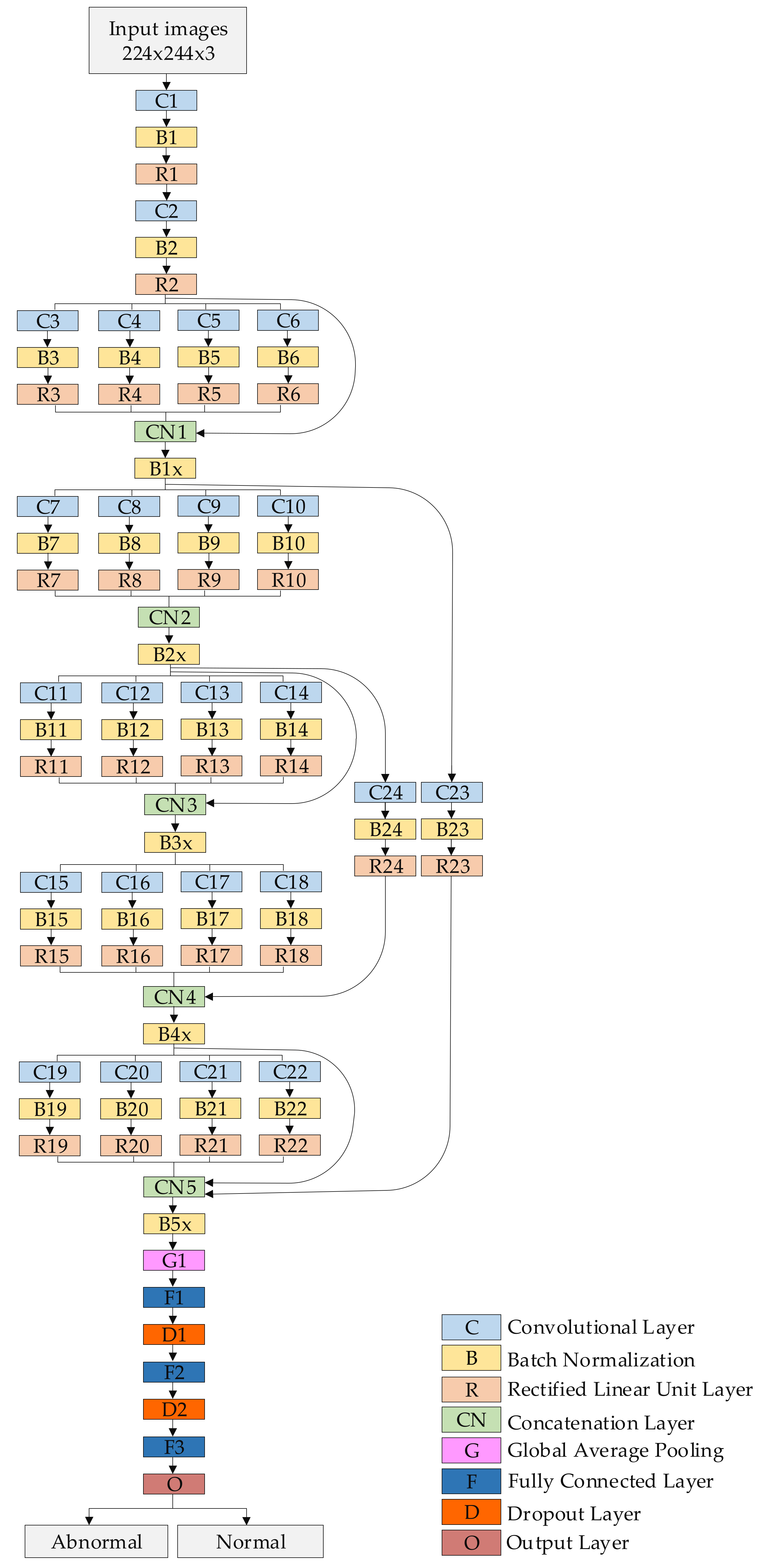
The procedure of transfer learning explained in Figure 7. The pre-trained models (VGG, ResNet) fellow the same procedure except for the first point.

5.4. Proposed Model

We have designed our hybrid model based on the study of previous state-of-the-art architectures and the advantages of each architecture. It integrates three different ideas involving traditional convolutions, parallel convolutions, and residual connections. The total number of layers of the proposed model is 91, which are explained in

Table 1. Our model architecture, C refers to convolutional layer, B refers to batch normalization Layer, R refers to rectified linear unit layer, CN refers to concatenation layer, G refers to global average pooling layer, D refers to dropout layer, F refers to the fully connected layer.

Name of Layer	Filter Size (FS) and Stride (S)	Activations
Input layer	-	224 × 224 × 3
C1, B1, R1	FS = 3 × 3, S = 1	224 × 224 × 16
C2, B2, R2	FS = 5 × 5, S = 2	112 × 112 × 16
C3, B3, R3	FS = 1 × 1, S = 1	112 × 112 × 16
C4, B4, R4	FS = 3 × 3, S = 1	112 × 112 × 16
C5, B5, R5	FS = 5 × 5, S = 1	112 × 112 × 16
C6, B6, R6	FS = 7 × 7, S = 1	112 × 112 × 16
CN1	Five inputs	112 × 112 × 80
B1x	Batch Normalization Layer	112 × 112 × 80
C7, B7, R7	FS = 1 × 1, S = 2	56 × 56 × 32
C8, B8, R8	FS = 3 × 3, S = 2	56 × 56 × 32
C9, B9, R9	FS = 5 × 5, S = 2	56 × 56 × 32
C10, B10, R10	FS = 7 × 7, S = 2	56 × 56 × 32
CN2	Four inputs	56 × 56 × 128
B2x	Batch Normalization Layer	56 × 56 × 128
C11, B11, R11	FS = 1 × 1, S = 1	56 × 56 × 32
C12, B12, R12	FS = 3 × 3, S = 1	56 × 56 × 32
C13, B13, R13	FS = 5 × 5, S = 1	56 × 56 × 32
C14, B14, R14	FS = 7 × 7, S = 1	56 × 56 × 32
CN3	Five inputs	56 × 56 × 256
B3x	Batch Normalization Layer	56 × 56 × 256
C15, B15, R15	FS = 1 × 1, S = 2	28 × 28 × 64
C16, B16, R16	FS = 3 × 3, S = 2	28 × 28 × 64
C17, B17, R17	FS = 5 × 5, S = 2	28 × 28 × 64
C18, B18, R18	FS = 7 × 7, S = 2	28 × 28 × 64
CN4	Five inputs	28 × 28 × 272
B4x	Batch Normalization Layer	28 × 28 × 272
C19, B19, R19	FS = 1 × 1, S = 1	28 × 28 × 128
C20, B20, R20	FS = 3 × 3, S = 1	28 × 28 × 128
C21, B21, R21	FS = 5 × 5, S = 1	28 × 28 × 128
C22, B22, R22	FS = 7 × 7, S = 1	28 × 28 × 128
CN5	Six inputs	28 × 28 × 800
B5x	Batch Normalization Layer	28 × 28 × 800
C23, B23, R23	FS = 5 × 5, S = 4	28 × 28 × 16
C24, B24, R24	FS = 3 × 3, S = 2	28 × 28 × 16
G1	-	1 × 1 × 800
F1	400 FC	1 × 1 × 400
D1	Dropout layer with learning rate:0.5	1 × 1 × 400
F2	200 FC	1 × 1 × 200
D2	Dropout layer with learning rate:0.5	1 × 1 × 200
F3	2 FC	1 × 1 × 2
O (Softmax function)	Normal, Abnormal	1 × 1 × 2

and Figure 8.

At the beginning of the model, we used two traditional convolutional layers with a filter size of 3 × 3 and 5 × 5 to reduce the input size of the input image. We chose these two filters to avoid losing small or large features. Picking a small filter size, such as 1 × 1, would act as a bottleneck that prevents large features passing through, which could help distinguish between classes; picking a large filter size, such as 11 × 11, would ignore small details that could lead to false classification. Therefore, we adopted average filter sizes. All convolutional layers in the model were followed by batch normalization and ReLU. Batch normalization speeds up the training progress, while the ReLU layer aids in reducing the effect of the vanishing gradient problem.

Traditional convolutional layers are followed by five blocks of parallel convolutional layers. Each block consists of four parallel convolutional layers with four different filter sizes (1 × 1, 3 × 3, 5 × 5, 7 × 7). The output of these four layers is combined in the concatenation layer to pass to the next block. The blocks are connected with long and short connections. The benefits of this type of combination are that it can integrate different levels of features and learn both small and large details, as having a variety of filter sizes. Furthermore, this structure is very helpful for gradient propagation as the error can backpropagate from multiple paths.

We employed a global average pooling layer on top of the five blocks of convolutional layers. Subsequently, three fully connected layers with two dropout layers were employed. Lastly, Softmax was adapted to produce the output. The global average pooling and dropout layers were used to overcome the issue of overfitting.

5.5. Training Scenarios

We utilized different training scenarios.

• Scenario 1: Training the proposed model from scratch with original images from target datasets.
  • Training with Dataset A
  • Training with Dataset B
• Scenario 2: Training the proposed model with Dataset C for TL purpose then fine-tuning the model to train it with A and B from Scenario 1.
• Scenario 3: Training the proposed model with Dataset D for TL purpose then fine-tuning the model to train it with A and B from Scenario 1.
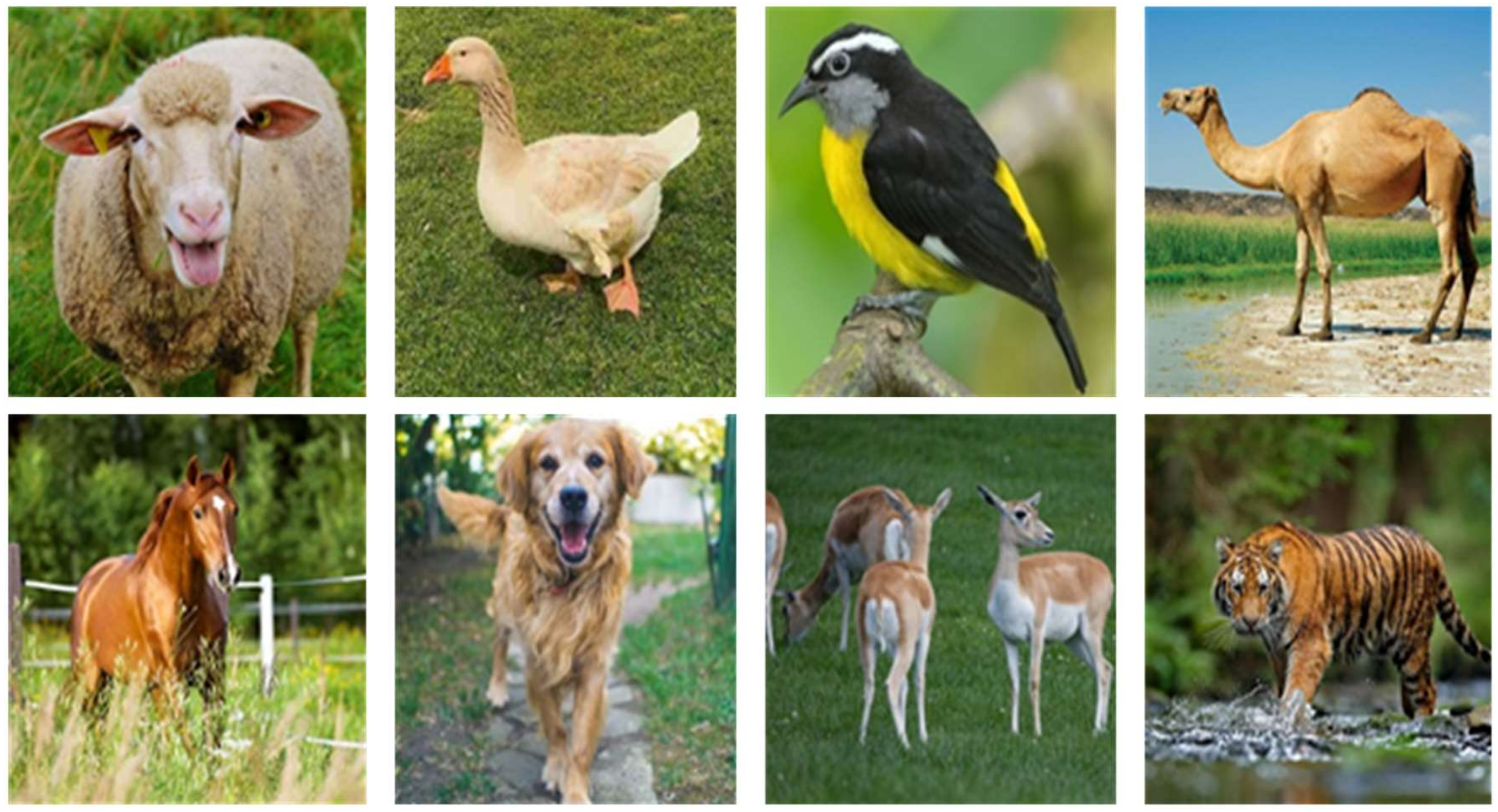
• Scenario 4: Fine-tuning two pre-trained state-of-the-art models (VGG19, ResNet50) then training them with A and B from Scenario 1. These two models had previously been trained with the ImageNet dataset containing nature images.

We achieved the visualization stage by showing what the first convolutional layer learned in our model trained in Scenario 2, Dataset A. Figure 9 shows learned filters of the abnormal class. Figure 10 shows the learned filter of the normal class. The training process was accomplished using stochastic gradient descent with momentum set to 0.9. The mini-batch size was 64 and MaxEpochs was 100, with a learning rate that was initially set to 0.001. We implemented our experiments on Matlab2019 as software and a processor from Intel (R) Core TM i7-5829K CPU @ 3.30 GHz, 32 GB RAM, and 8 GB GPU.

6. Experimental Results

The evaluation stage was achieved by calculating recall, precision, and F1-score, where TP refers to true positives, FP refers to false positives, and FN refers to false negatives. These parameters are defined as:

Recall = TP/ (TP+FN)

(1)

Precision = TP/ (TP+FP)

(2)

F1 _score = 2 × ((Precision × Recall) / (Precision + Recall)

(3)

We started by evaluating the proposed model performance with target datasets trained with Scenario 1, as reported in

Table 2. Results of two target datasets with Scenario 1.

Target Dataset	Precision (%)	Recall (%)	F1-Score (%)
Dataset A	84.8	88.6	86.6
Dataset B	82.9	87.5	85.1

.

The results of the proposed model with Dataset A are slightly higher than those with Dataset B, achieving 84.8%, 88.6%, and 86.6% for precision, recall, and F1-score, respectively. The proposed model with Dataset B achieved 82.9% for precision, 87.5% for recall, and 85.1% for the F1-score. Although the performance of the proposed model with Dataset A was higher than the proposed model with Dataset B, both still roughly had the same performance.

In Scenario 2, TL from medical sources (Dataset C) was adopted and the results are listed in

Table 3. Results of two target datasets with Scenario 2.

Target Dataset	Precision (%)	Recall (%)	F1-Score (%)
Dataset A	96.8	98.6	97.6
Dataset B	81.8	86.7	84.1

.

The results of the proposed model with Dataset A were significantly higher than those with Dataset B, achieving 96.8%, 98.6%, and 97.6% for precision, recall, and F1-score, respectively. By comparing the performance of the proposed model with Dataset A in Scenario 2 to Scenario 1, there was a remarkable improvement in the performance of Scenario 2 due to the TL from the same domain of Dataset A. On the other hand, the situation was different with Dataset B in Scenario 2 compared to Scenario 1. Employing TL from a medical source for animal classification (Dataset B) degraded the performance due to differences in learned features. The proposed model with dataset B achieved 81.8% for precision, 86.7% for recall and 84.1% for the F1-score. In these situations, training from scratch is preferable as in Scenario 1.

In Scenario 3, the source of TL was in the same domain of Dataset B, which boosted the results to 91.6%, 96.9%, and 94.1% for precision, recall, and F1-score, respectively. By comparing the performance of the proposed model with Dataset B in Scenario 3 to that of Dataset B in Scenarios 1 and 2, it was clear that the same domain transfer played a big role in enhancing performance. Although the performance of the proposed model with Dataset A was less than that with Dataset B in Scenario 3, the results of the proposed model with Dataset A slightly improved compared to the results from Scenario 1. It achieved 86.5% for precision, 92.7% for recall and 89.4% for the F1-score. These results are still less than the results from Scenario 2. The results of the proposed model with Datasets A and B trained in Scenario 3 are listed in

Table 4. Results of two target datasets with Scenario 3.

Target Dataset	Precision (%)	Recall (%)	F1- score (%)
Dataset A	86.5	92.7	89.4
Dataset B	91.6	96.9	94.1

.

In

Table 5. Results of two target datasets with Scenario 4.

Models	Target Dataset	Precision (%)	Recall (%)	F1- score (%)
VGG19	Dataset A	86.4	90.5	88.4
	Dataset B	89.3	95.2	92.1
ResNet50	Dataset A	88.2	93.1	90.5
	Dataset B	93.7	98.9	96.2

, we employed two state-of-the-art models trained on the ImageNet dataset, which consists of natural images including animals. Both the ImageNet dataset and Dataset B are in the same domain. For that reason, the results of Dataset B were higher than the results of Dataset A with a score 89.3% for precision, 95.2% for recall and 92.1% for the F1-score with VGG19, while it scored 93.7% for precision, 98.9% for recall, and 96.2% for the F1-score with ResNet50. The results of ResNet50 with Dataset B were considered the dataset’s highest results due to training with the ImageNet dataset as source of TL and the results of the proposed model in Scenario 3 were the second highest. It showed the importance of the same domain of transfer learning. On the other hand, the results of these models on Dataset A improved compared to Scenario 1 by achieving 86.4% for precision, 90.5% for recall and 88.4% for the F1-score with VGG19, while it achieved 88.2% for precision, 93.1% for recall and 90.5% for the F1-score with ResNet50. Although these models (VGG19, ResNet50) were trained with one million images, they were not from the same domain as the medical images. Therefore, a fewer number of images for TL in the same domain is better than a million images in a different domain. In Scenario 2, TL from the same domain significantly improved performance with fewer images than the million images that VGG 19 and ResNet50 were trained with.

7. Conclusions

In summarizing this paper, there are six main highlights: (i) the issue of the lack of training has been tackled using transfer learning; (ii) a hybrid deep learning model has been proposed combining different structures including traditional and parallel convolutional layers along with residual links. Due to this type of structure, the proposed model has the advantage of better feature representation; (iii) a DFU dataset was collected and labeled as normal or abnormal by an expert in the field and utilized for experiment; and (iv) four training scenarios were designed including training from scratch and training scenarios representing the same and different domain TL for target datasets. Four datasets were employed for the training scenarios including two target datasets and two other datasets for TL purposes; (v) the same domain TL was proven to be more beneficial for addressing the lack of training issue. It was found that fewer images in the same domain of the target dataset were better than a large number of images from a different domain; (vi) the proposed model with the DFU dataset (Dataset A) achieved an F1-score of 86.6% with training from scratch, 89.4% with TL from a different domain of the target dataset, and 97.6% with TL from the same domain of the target dataset. As the idea of the same domain TL improved performance, we plan to adopt it in other applications.

References

1. Shahbazian, H.; Yazdanpanah, L.; Latifi, S.M. Risk assessment of patients with diabetes for foot ulcers according to risk classification consensus of International Working Group on Diabetic Foot (IWGDF). Pak. J. Med. Sci. 2013, 23, 730. [Google Scholar] [CrossRef]
2. Ramachandran, A.; Snehalatha, C.; Shetty, A.S.; Nanditha, A. Trends in prevalence of diabetes in Asian countries. World J. Diabetes 2012, 3, 110. [Google Scholar] [CrossRef] [PubMed]
3. Shaw, J.E.; Sicree, R.A.; Zimmet, P.Z. Global estimates of the prevalence of diabetes for 2010 and 2030. Diabetes Res. Clin. Pract. 2010, 87, 4–14. [Google Scholar] [CrossRef] [PubMed]
4. Whiting, D.R.; Guariguata, L.; Weil, C.; Shaw, J. IDF diabetes atlas: Global estimates of the prevalence of diabetes for 2011 and 2030. Diabetes Res. Clin. Pract. 2011, 94, 311–321. [Google Scholar] [CrossRef]
5. Aalaa, M.; Malazy, O.T.; Sanjari, M.; Peimani, M.; Mohajeri-Tehrani, M.R. Nurses’ role in diabetic foot prevention and care; a review. J. Diabetes Metab. Disord. 2012, 11, 24. [Google Scholar] [CrossRef] [PubMed] [Green Version]
6. Alavi, A.; Sibbald, R.G.; Mayer, D.; Goodman, L.; Botros, M.; Armstrong, D.G.; Woo, K.; Boeni, T.; Ayello, E.A.; Kirsner, R.S. Diabetic foot ulcers: Part II. Management. J. Am. Acad. Dermatol. 2014, 70, 21.e1–21.e24. [Google Scholar] [CrossRef] [PubMed]
7. Cavanagh, P.R.; Lipsky, B.A.; Bradbury, A.W.; Botek, G. Treatment for diabetic foot ulcers. Lancet 2005, 366, 1725–1735. [Google Scholar] [CrossRef]
8. Leone, S.; Pascale, R.; Vitale, M.; Esposito, S. Epidemiology of diabetic foot. Infez Med 2012, 20, 8–13. [Google Scholar]
9. Richard, J.L.; Schuldiner, S. Epidemiology of diabetic foot problems. Rev. Med. Interne 2008, 29, S222–S230. [Google Scholar] [CrossRef]
10. Nather, A.; Bee, C.S.; Huak, C.Y.; Chew, J.L.; Lin, C.B.; Neo, S.; Sim, E.Y. Epidemiology of diabetic foot problems and predictive factors for limb loss. J. Diabetes Complicat. 2008, 22, 77–82. [Google Scholar] [CrossRef]
11. Bakri, F.G.; Allan, A.H.; Khader, Y.S.; Younes, N.A.; Ajlouni, K.M. Prevalence of diabetic foot ulcer and its associated risk factors among diabetic patients in Jordan. Jordan Med. J. 2012, 171, 1–16. [Google Scholar]
12. Iraj, B.; Khorvash, F.; Ebneshahidi, A.; Askari, G. Prevention of diabetic foot ulcer. Int. J. Prev. Med. 2013, 4, 373. [Google Scholar] [PubMed]
13. Fard, A.S.; Esmaelzadeh, M.; Larijani, B. Assessment and treatment of diabetic foot ulcer. Int. J. Clin. Pract. 2007, 61, 1931–1938. [Google Scholar] [CrossRef] [PubMed]
14. Snyder, R.J.; Hanft, J.R. Diabetic foot ulcers—Effects on quality of life, costs, and mortality and the role of standard wound care and advanced-care therapies in healing: A review. Ostomy/Wound Manag. 2009, 55, 28–38. [Google Scholar]
15. Liu, C.; van Netten, J.J.; Van Baal, J.G.; Bus, S.A.; van Der Heijden, F. Automatic detection of diabetic foot complications with infrared thermography by asymmetric analysis. J. Biomed. Opt. 2015, 20, 026003. [Google Scholar] [CrossRef] [Green Version]
16. Van Netten, J.J.; Prijs, M.; van Baal, J.G.; Liu, C.; van Der Heijden, F.; Bus, S.A. Diagnostic values for skin temperature assessment to detect diabetes-related foot complications. Diabetes Technol. Ther. 2014, 16, 714–721. [Google Scholar] [CrossRef] [Green Version]
17. Wang, L.; Pedersen, P.C.; Agu, E.; Strong, D.M.; Tulu, B. Area determination of diabetic foot ulcer images using a cascaded two-stage SVM-based classification. IEEE Trans. Biomed. Eng. 2016, 64, 2098–2109. [Google Scholar] [CrossRef]
18. Goyal, M.; Yap, M.H.; Reeves, N.D.; Rajbhandari, S.; Spragg, J. Fully convolutional networks for diabetic foot ulcer segmentation. In Proceedings of the International Conference on Systems, Man, and Cybernetics (SMC), Banff, AB, Canada, 5–8 October 2017; pp. 618–623. [Google Scholar]
19. Wannous, H.; Lucas, Y.; Treuillet, S. Enhanced assessment of the wound-healing process by accurate multiview tissue classification. IEEE Trans. Med. Imaging 2010, 30, 315–326. [Google Scholar] [CrossRef] [Green Version]
20. Kolesnik, M.; Fexa, A. Multi-dimensional color histograms for segmentation of wounds in images. In Proceedings of the International Conference Image Analysis and Recognition, Toronto, ON, Canada, 28–30 September 2005; Springer: Berlin/Heidelberg, Germany; pp. 1014–1022. [Google Scholar]
21. Kolesnik, M.; Fexa, A. How robust is the SVM wound segmentation? In Proceedings of the 7th Nordic Signal Processing Symposium-NORSIG, Reykjavik, Iceland, 7–9 June 2006; pp. 50–53. [Google Scholar]
22. Veredas, F.; Mesa, H.; Morente, L. Binary tissue classification on wound images with neural networks and bayesian classifiers. IEEE Trans. Med. Imaging 2010, 29, 410–427. [Google Scholar] [CrossRef]
23. LeCun, Y.; Bengio, Y.; Hinton, G. Deep learning. Nature 2015, 521, 436–444. [Google Scholar] [CrossRef]
24. Bajwa, M.N.; Muta, K.; Malik, M.I.; Siddiqui, S.A.; Braun, S.A.; Homey, B.; Dengel, A.; Ahmed, S. Computer-aided diagnosis of skin diseases using deep neural networks. Appl. Sci. 2020, 10, 2488. [Google Scholar] [CrossRef] [Green Version]
25. Alzubaidi, L.; Fadhel, M.A.; Al-Shamma, O.; Zhang, J.; Duan, Y. Deep learning models for classification of red blood cells in microscopy images to aid in sickle cell anemia diagnosis. Electronics 2020, 9, 427. [Google Scholar] [CrossRef] [Green Version]
26. Luján-García, J.E.; Yáñez-Márquez, C.; Villuendas-Rey, Y.; Camacho-Nieto, O. A transfer learning method for pneumonia classification and visualization. Appl. Sci. 2020, 10, 2908. [Google Scholar] [CrossRef] [Green Version]
27. Alzubaidi, L.; Al-Shamma, O.; Fadhel, M.A.; Zhang, J.; Duan, Y. Optimizing the performance of breast cancer classification by employing the same domain transfer learning from hybrid deep convolutional neural network model. Electronics 2020, 9, 445. [Google Scholar] [CrossRef] [Green Version]
28. Goyal, M.; Reeves, N.D.; Davison, A.K.; Rajbhandari, S.; Spragg, J.; Yap, M.H. DFUNET: Convolutional neural networks for diabetic foot ulcer classification. IEEE Trans. Emerg. Top. Comput. Intell. 2018, 1–12. [Google Scholar] [CrossRef] [Green Version]
29. Alzubaidi, L.; Fadhel, M.A.; Oleiwi, S.R.; Al-Shamma, O.; Zhang, J. DFU_QUTNet: Diabetic foot ulcer classification using novel deep convolutional neural network. Multimed. Tools Appl. 2020, 79, 15655–15677. [Google Scholar] [CrossRef]
30. Krizhevsky, A.; Sutskever, I.; Hinton, G.E. ImageNet classification with deep convolutional neural networks. In Proceedings of the Advances in Neural Information Processing Systems, Lake Tahoe, NV, USA, 3–6 December 2012; pp. 1097–1105. [Google Scholar]
31. Wang, J.; Yang, J.; Yu, K.; Lv, F.; Huang, T.; Gong, Y. Locality-constrained linear coding for image classification. In Proceedings of the IEEE Computer Society Conference on Computer Vision and Pattern Recognition, San Francisco, CA, USA, 13–18 June 2010; pp. 3360–3367. [Google Scholar]
32. Rasheed, N.; Khan, S.A.; Khalid, A. Tracking and abnormal behavior detection in video surveillance using optical flow and neural networks. In Proceedings of the 28th International Conference on Advanced Information Networking and Applications Workshops, Victoria, BC, Canada, 13–16 May 2014; pp. 61–66. [Google Scholar]
33. Geiger, A.; Lauer, M.; Wojek, C.; Stiller, C.; Urtasun, R. 3D traffic scene understanding from movable platforms. IEEE Trans. Pattern Anal. Mach. Intell. 2014, 36, 1012–1025. [Google Scholar] [CrossRef] [Green Version]
34. Wu, Y.; Lim, J.; Yang, M.-H. Object tracking benchmark. IEEE Trans. Pattern Anal. Mach. Intell. 2015, 37, 1834–1848. [Google Scholar] [CrossRef] [Green Version]
35. He, K.; Zhang, X.; Ren, S.; Sun, J. Deep residual learning for image recognition. In Proceedings of the IEEE Conference on Computer Vision and Pattern Recognition, Las Vegas, NV, USA, 27–30 June 2016; pp. 770–778. [Google Scholar]
36. Weinberger, K.; Saul, L. Distance metric learning for large margin nearest neighbor classification. J. Mach. Learn. Res. 2009, 10, 207–244. [Google Scholar]
37. Simonyan, K.; Zisserman, A. Very deep convolutional networks for large-scale image recognition. arXiv 2014, arXiv:1409.1556. [Google Scholar]
38. Fung, G.; Mangasarian, O.L.; Shavlik, J. Knowledge-based support vector machine classifiers. In The Neural Information Processing Systems Foundation (NIPS 2002); MIT Press: Cambridge, MA, USA, 2002; pp. 521–528. [Google Scholar]
39. Szegedy, C.; Liu, W.; Jia, Y.; Sermanet, P.; Reed, S.; Anguelov, D.; Erhan, D.; Vanhoucke, V.; Rabinovich, A. Going deeper with convolutions. In Proceedings of the IEEE Conference on Computer Vision and Pattern Recognition, Boston, MA, USA, 7–12 June 2015; pp. 1–9. [Google Scholar]
40. Simonyan, K.; Vedaldi, A.; Zisserman, A. Deep inside convolutional networks: Visualising image classification models and saliency maps. In Proceedings of the International Conference on Learning Representations Workshop, Banff, AB, Canada, 14–16 April 2014; pp. 1–8. [Google Scholar]
41. Zeiler, M.D.; Fergus, R. Visualizing and understanding convolutional networks. In Proceedings of the European Conference on Computer Vision, Zurich, Switzerland, 6–12 September 2014; pp. 818–833. [Google Scholar]
42. Bengio, Y. Learning deep architectures for AI. Found. Trends Mach. Learn. 2009, 2, 1–127. [Google Scholar] [CrossRef]
43. Cireşan, D.; Meier, U.; Schmidhuber, J. Multi-column deep neural networks for image classification. In Proceedings of the IEEE Conference on Computer Vision and Pattern Recognition, Providence, RI, USA, 16–21 June 2012; pp. 3642–3649. [Google Scholar]
44. Rawat, W.; Wang, Z. Deep convolutional neural networks for image classification: A comprehensive review. Neural Comput. 2017, 29, 2352–2449. [Google Scholar] [CrossRef]
45. Guo, J.; Zhang, S.; Li, J. Hash learning with convolutional neural networks for semantic based image retrieval. In Proceedings of the Pacific-Asia Conference Knowledge Discovery Data Mining, Auckland, New Zealand, 19–22 April 2016; pp. 227–238. [Google Scholar]
46. Girshick, R.; Donahue, J.; Darrell, T.; Malik, J. Region-based convolutional networks for accurate object detection and semantic segmentation. IEEE Trans. Pattern Anal. Mach. Intell. 2016, 38, 142–158. [Google Scholar] [CrossRef] [PubMed]
47. Koziarski, M.; Cyganek, B. Image recognition with deep neural networks in presence of noise—Dealing with and taking advantage of distortions. Integr. Comput. Aided Eng. 2017, 24, 337–349. [Google Scholar] [CrossRef]
48. Shang, W.; Sohn, K.; Almeida, D.; Lee, H. Understanding and improving convolutional neural networks via concatenated rectified linear units. In Proceedings of the 33rd International Conference on International Conference on Machine Learning (ICML), New York, NY, USA, 19–24 June 2016; pp. 3276–3284. [Google Scholar]
49. Srivastava, N.; Hinton, G.; Krizhevsky, A.; Sutskever, I.; Salakhutdinov, R. Dropout: A simple way to prevent neural networks from overfitting. J. Mach. Learn. Res. 2014, 15, 1929–1958. [Google Scholar]
50. Ioffe, S.; Szegedy, C. Batch normalization: Accelerating deep network training by reducing internal covariate shift. In Proceedings of the International Conference on International Conference on Machine Learning, Lille, France, 6–11 July 2015; pp. 448–456. [Google Scholar]
51. Lv, E.; Wang, X.; Cheng, Y.; Yu, Q. Deep convolutional network based on pyramid architecture. IEEE Access 2018, 6, 43125–43135. [Google Scholar] [CrossRef]
52. Targ, S.; Almeida, D.; Lyman, K. ResNet in ResNet: Generalizing residual architectures. arXiv 2016, arXiv:1603.08029. [Google Scholar]
53. Zagoruyko, S.; Komodakis, N. Wide residual networks. arXiv 2016, arXiv:1605.07146. [Google Scholar]
54. Veit, A.; Wilber, M.J.; Belongie, S. Residual networks behave like ensembles of relatively shallow networks. In Proceedings of the Advances in Neural Information Processing Systems, Barcelona, Spain, 5–10 December 2016; pp. 550–558. [Google Scholar]
55. Szegedy, C.; Ioffe, S.; Vanhoucke, V.; Alemi, A. Inception-v4 Inception-ResNet and the impact of residual connections on learning. In Proceedings of the Thirty-First AAAI Conference on Artificial Intelligence, San Francisco, CA, USA, 4–9 February 2017. [Google Scholar]
56. Szegedy, C.; Vanhoucke, V.; Ioffe, S.; Shlens, J.; Wojna, Z. Rethinking the inception architecture for computer vision. In Proceedings of the IEEE Conference on Computer Vision and Pattern Recognition, Las Vegas, NV, USA, 27–30 June 2016; pp. 2818–2826. [Google Scholar]
57. Larsson, G.; Maire, M.; Shakhnarovich, G. FractalNet: Ultra-Deep Neural Networks Without Residuals. arXiv 2016, arXiv:1605.07648. [Google Scholar]
58. Zhao, L.; Wang, J.; Li, X.; Tu, Z.; Zeng, W. On the connection of deep fusion to ensembling. arXiv 2016, arXiv:1611.07718. [Google Scholar]
59. Wang, J.; Wei, Z.; Zhang, T.; Zeng, W. Deeply-fused nets. arXiv 2016, arXiv:1605.07716. [Google Scholar]
60. Deng, J.; Dong, W.; Socher, R.; Li, L.J.; Li, K.; Fei-Fei, L. ImageNet: A large-scale hierarchical image database. In Proceedings of the Conference on Computer Vision and Pattern Recognition, Miami, FL, USA, 20–25 June 2009; pp. 248–255. [Google Scholar]
61. Shin, H.; Roth, H.R.; Gao, M.; Lu, L.; Xu, Z.; Nogues, I.; Yao, J.; Mollura, D.; Summers, R.M. Deep convolutional neural networks for computer-aided detection: CNN architectures, dataset characteristics and transfer learning. IEEE Trans. Med. Imaging 2016, 35, 1285–1298. [Google Scholar] [CrossRef] [PubMed] [Green Version]
62. Tan, C.; Sun, F.; Kong, T.; Zhang, W.; Yang, C.; Liu, C. A survey on deep transfer learning. In Proceedings of the International Conference on Artificial Neural Networks, Rhodes, Greece, 4–7 October 2018; Springer: Cham, Switzerland; pp. 270–279. [Google Scholar]
63. Shorten, C.; Khoshgoftaar, T.M. A survey on image data augmentation for deep learning. J. Big Data 2019, 6, 60. [Google Scholar] [CrossRef]
64. Cook, D.; Feuz, K.D.; Krishnan, N.C. Transfer learning for activity recognition: A survey. Knowl. Inf. Syst. 2013, 36, 537–556. [Google Scholar] [CrossRef] [PubMed] [Green Version]
65. Cao, X.; Wang, Z.; Yan, P.; Li, X. Transfer learning for pedestrian detection. Neurocomputing 2013, 100, 51–57. [Google Scholar] [CrossRef]
66. Raghu, M.; Zhang, C.; Kleinberg, J.; Bengio, S. Transfusion: Understanding transfer learning for medical imaging. In Proceedings of the Neural Information Processing Systems, Vancouver, BC, Canada, 8–14 December 2019; pp. 3342–3352. [Google Scholar]
67. Animals. Available online: https://www.kaggle.com/alessiocorrado99/animals10#translate.py (accessed on 15 January 2020).
68. Wounds. Available online: https://github.com/produvia/deep-learning-for-wound-care. (accessed on 15 January 2020).
69. Clinical Skin Disease. Available online: https://medicine.uiowa.edu/dermatology/education/clinical-skin-disease-images (accessed on 15 January 2020).
70. Codella, N.; Rotemberg, V.; Tschandl, P.; Celebi, M.E.; Dusza, S.; Gutman, D.; Helba, B.; Kalloo, A.; Liopyris, K.; Marchetti, M.; et al. A Skin lesion analysis toward melanoma detection 2018: A challenge hosted by the international skin imaging collaboration (ISIC). arXiv 2019, arXiv:1902.03368. [Google Scholar]
71. Combalia, M.; Codella, N.C.; Rotemberg, V.; Helba, B.; Vilaplana, V.; Reiter, O.; Carrera, C.; Barreiro, A.; Halpern, A.C.; Puig, S.; et al. BCN20000: Dermoscopic lesions in the wild. arXiv 2019, arXiv:1908.02288. [Google Scholar]
72. Animals1. Available online: https://www.kaggle.com/nafisur/dogs-vs-cats (accessed on 22 January 2020).
73. Animals2. Available online: https://www.kaggle.com/gpiosenka/100-bird-species (accessed on 22 January 2020).
74. Animals3. Available online: https://www.kaggle.com/navneetsurana/animaldataset (accessed on 22 January 2020).
75. Lin, M.; Chen, Q.; Yan, S. Network in network. arXiv 2013, arXiv:1312.4400. [Google Scholar]
Figure 1. Sample from diabetic foot ulcer (DFU) dataset (Dataset A) of normal and abnormal region with a size of 224 × 224. The blue color is abnormal patch (DFU) class, green color is normal class.
Applsci 10 04523 g001
Figure 2. Samples from animal dataset (Dataset B) (first row is chicken class; second row is cow class).
Applsci 10 04523 g002
Figure 3. Samples from the medical dataset (Dataset C).
Applsci 10 04523 g003
Figure 4. Samples from the large animal dataset (Dataset D).
Applsci 10 04523 g004
Figure 5. Pooling operations.
Applsci 10 04523 g005
Figure 6. The concept of the transfer learning.
Applsci 10 04523 g006
Figure 7. Transfer leaning pipeline.
Applsci 10 04523 g007
Figure 8. The proposed model architecture.
Applsci 10 04523 g008
Figure 9. Learned filters of the abnormal class (DFU).
Applsci 10 04523 g009
Figure 10. The learned filter of the normal class.
Applsci 10 04523 g010