Robust Adaptive Control for Nonlinear Aircraft System with Uncertainties

Abstract

Model reference adaptive control (MRAC) schemes are known as an effective method to deal with system uncertainties. High adaptive gains are usually needed in order to achieve fast adaptation. However, this leads to high-frequency oscillation in the control signal and may even make the system unstable. A robust adaptive control architecture was designed in this paper for nonlinear aircraft dynamics facing the challenges of input uncertainty, matched uncertainty, and unmatched uncertainty. By introducing a robust compensator to the MRAC framework, the high-frequency components in the control response were eliminated. The proposed control method was applied to the longitudinal-direction motion control of a nonlinear aircraft system. Flight simulation results demonstrated that the proposed robust adaptive method was able to achieve fast adaptation without high-frequency oscillations, and guaranteed transient performance.

1. Introduction

Uncertain nonlinear system control is a challenging topic in the field of control theory and application. Fundamental control methods for nonlinear systems include the back-stepping approach [1], feedback control [2], and sliding mode control [3]. Additionally, adaptive control has attracted much attention due to its capacity to accommodate system uncertainties. Various adaptive strategies have been developed for uncertain nonlinear systems, such as adaptive optimal control [4], immersion and invariance (I & I) adaptive control [5], adaptive neural control [6], and adaptive sliding mode control [7]. Model reference adaptive control (MRAC) is an important area in aircraft system control research.

MRAC architecture was developed in the 1950s [8] for the design of aircraft autopilot to deal with uncertainties during the flight period. This control scheme has been extensively investigated in aerospace engineering [9,10,11,12], since the controller design does not rely excessively on accurate plant models. In standard MRAC, high adaptive gains are generally employed to achieve fast adaptation in the existence of system uncertainties. However, this leads to high-frequency oscillations in system responses, which can be a potential threat to system stability.

Specifically, high-performance safety-critical aircraft require the designed controller to have the ability to guarantee the transient performance of the system while achieving fast adaptation. In the MRAC structure, the tracking error between a real uncertain plant and the selected reference model plays a decisive role in the performance of the adaptive controller, in that the controller parameters are adjusted online for the update law, which is designed on the basis of tracking errors. When large uncertainties exist in the aircraft system, such as control surface failure, aerodynamic coefficient changes, or unexpected external disturbances, high adaptive gains are applied to rapidly reduce system tracking errors in order to achieve fast adaptation, which offsets the impact of uncertainties. High adaptive gains, however, may introduce high-frequency components into the control response, and a closed-loop system with poor transient behavior in the early stage of adaptation will in turn suffer from issues of actuator saturation [13], unmodeled dynamics [14], and even instability of the system [15].

In view of this defect of MRAC, great efforts have been made to deal with the problem. Multiple models and switching strategies [16] were developed to improve the transient response of the adaptive control by choosing a model that best approximates the plant for the controller. A combined/composite-model-reference adaptive control system was reported [17,18,19], which used prediction errors to formulate adaptive laws; flight test results confirmed a noticeable improvement in transient performance with high adaptive gains. Cao et al. investigated the $L_1$ adaptive control method [20,21], wherein the high-frequency components in a control signal can be filtered out by a low-pass filter. A low-frequency learning adaptive control scheme [22,23] was also proposed to improve transient performance while achieving fast adaptation. An observer-based adaptive control scheme [24,25], in which an error feedback item is introduced to the reference model, was verified to be a practical approach for improving transient behavior. However, this resulted in changing the well-designed reference model, which meant that the desired reference signal to be tracked had to be revised.

In this paper, a robust adaptive control for handling control effectiveness uncertainty, matched plant uncertainty, and external disturbance uncertainty of an aircraft is presented. The main contribution of this paper is the improved tracking performance of a model reference adaptive control system. In order to restrain high-frequency oscillations of the control signal due to the fast adaptation, an error feedback compensator was designed as a robust controller, with the intent to minimize the influence of estimate parameter errors on system responses. Compared with existing approaches aiming to improve the transient performance of MRAC, our method does not require modification of the standard adaptive law or the selected reference model, which means that our approach is easier to implement in engineering contexts. First, a standard MRAC architecture was designed with a baseline controller. Second, a robust compensator was adopted in order to resist high-frequency oscillations while achieving fast adaptation. The robust $H_{\infty }$ control theory was applied for the robust controller design, and the robust feedback gain was calculated by solving linear matrix inequality.

The rest of the paper is organized as follows. In Section 2, the control problem is formulated. Section 3 presents the design procedure of the proposed robust adaptive controller and analyses of the stability of the closed-loop system. Section 4 displays the response of the uncertain nonlinear system with the designed controller, using flight control simulations for an aircraft model. Section 5 concludes the paper.

2. Problem Formulation

The nonlinear aircraft dynamics, containing input uncertainty, matched uncertainty, and unmatched disturbance, is given by

$$\{\begin{array}{l}{\dot{x}}_p\left(t\right)=A_p{x}_p\left(t\right)+B_p\left(\mathsf{\Lambda }u\left(t\right)+{\theta }_p^T{\mathsf{\Theta }}_p\left(x_p\left(t\right)\right)\right)+d_p\left(t\right)\hfill \\ y_p\left(t\right)=C_p{x}_p\left(t\right)\hfill \end{array}$$

(1)

where $x_p\in {ℝ}^{n_p}$ is the plant state, $u\in {ℝ}^m$ is the control input, and $y_p\in {ℝ}^l$ is the measurement output of the system. $A_p\in {ℝ}^{n_p\times n_p}$, $B_p\in {ℝ}^{n_p\times m}$, and $C_p\in {ℝ}^{l\times n_p}$ are constant known matrices. In practical flight applications [26], the state matrix $A_p$ is generally obtained by wind-tunnel measurements. $C_p$ can be determined through the relationship between output and state. However, the input matrix $B_p$ may be inaccurate for the nominal system due to damage and failures, or due to changes in aircraft dynamics. The actuator anomaly can be modeled as an unknown element $\mathsf{\Lambda }\in {ℝ}^{m\times m}$, representing the uncertain control effectiveness. $\mathsf{\Lambda }$ is nonsingular, which has upper bounds known a priori: $\sigma =\sup \Vert \mathsf{\Lambda }\Vert$. ${\theta }_p^T{\mathsf{\Theta }}_p\left(x\right)\in {ℝ}^{m\times n_p}$ represents the matched uncertainty that enters the system through the columns of $B_p$. ${\theta }_p\in {ℝ}^{s\times m}$ is the unknown constant weight matrix, and ${\mathsf{\Theta }}_p(\cdot ):{ℝ}^{n_p}\to {ℝ}^s$ is a vector of the basic functions that can be described as ${\mathsf{\Theta }}_p\left(x_p\right)={\left[{\varphi }_{p1}\left(x_p\right),{\varphi }_{p2}\left(x_p\right),\dots ,{\varphi }_{ps}\left(x_p\right)\right]}^T$. $d_p\in {ℝ}^{n_p}$ represents the unmatched bounded disturbance uncertainty in the flight period; i.e., ${\sup }_{\forall t}\left|\right|d_p\left|\right|\le d_0$.

Our goal was to design a control input $u\left(t\right)$ that would make $y_p\left(t\right)$ track a reference command $r\left(t\right)$ with bounded errors in the presence of uncertainties $\mathsf{\Lambda }$, ${\theta }_p$, and $d_p$. Furthermore, we assumed that the pair $\left(\begin{array}{cc}{A}_p& B_p\end{array}\right)$ was controllable, $x_p\left(t\right)$ was available for feedback, and $u\left(t\right)$ was the class of admissible controls consisting of measurable functions.

3. Controller Design

3.1. State Augmentation

Considering that the integral action was able to handle set-point tracking and disturbance rejection issues, the output signal tracking error was defined as follows.

$${\dot{x}}_e\left(t\right)=r\left(t\right)-y_p\left(t\right)$$

(2)

where $r\left(t\right)\in {ℝ}^l$ is a bounded piecewise continuous tracking command.

This integral error state was then appended to the plant model in Equation (1); therefore, the augmented dynamics were delivered as

$$\{\begin{array}{l}\left[\begin{array}{c}{\dot{x}}_p\left(t\right)\\ {\dot{x}}_e\left(t\right)\end{array}\right]=\left[\begin{array}{cc}{A}_p& 0\\ -C_p& 0\end{array}\right]\left[\begin{array}{c}{x}_p\left(t\right)\\ x_e\left(t\right)\end{array}\right]+\left[\begin{array}{c}{B}_p\\ 0\end{array}\right]\left(\mathsf{\Lambda }u\left(t\right)+{\theta }_p^T{\mathsf{\Theta }}_p\left(x_p\left(t\right)\right)\right)+\left[\begin{array}{c}{d}_p\left(t\right)\\ 0\end{array}\right]+\left[\begin{array}{c}0\\ I\end{array}\right]r\left(t\right)\\ y_p\left(t\right)=\left[\begin{array}{cc}{C}_p& 0\end{array}\right]\left[\begin{array}{c}{x}_p\left(t\right)\\ x_e\left(t\right)\end{array}\right]\end{array}$$

(3)

Define $x\left(t\right)={\left[x_p\left(t\right),x_e\left(t\right)\right]}^T$ and $n=n_p+l$, so $x\left(t\right)\in {ℝ}^n$. Equation (3) can be rewritten as

$$\{\begin{array}{l}\dot{x}\left(t\right)=Ax\left(t\right)+B\left(\mathsf{\Lambda }u\left(t\right)+{\theta }^T\mathsf{\Theta }\left(x\left(t\right)\right)\right)+d\left(t\right)+B_{r}r\left(t\right)\\ y\left(t\right)=Cx\left(t\right)\end{array}$$

(4)

where

$$A=\left[\begin{array}{cc}{A}_p& 0\\ -C_p& 0\end{array}\right],B=\left[\begin{array}{c}{B}_p\\ 0\end{array}\right],B_r=\left[\begin{array}{c}0\\ I\end{array}\right],C=\left[\begin{array}{cc}{C}_p& 0\end{array}\right]$$

3.2. Reference Model

The reference model was selected as

$$\{\begin{array}{l}{\dot{x}}_m\left(t\right)=A_m{x}_m\left(t\right)+B_{r}r\left(t\right)\\ y_m\left(t\right)=C{x}_m\left(t\right)\end{array}$$

(5)

where $x_m\left(t\right)\in {ℝ}^n$ is the reference state vector and $A_m\in {ℝ}^{n\times n}$ is Hurwitz. Since $r\left(t\right)$ is bounded, it follows that $x_m\left(t\right)$ and $y_m\left(t\right)$ are uniformly bounded for all $x_m\left(0\right)$.

3.3. Controller Design

The main purpose of the controller was to track the reference command $r\left(t\right)$ with the existence of the uncertainties $\mathsf{\Lambda }$, ${\theta }^T$, and $d$. A traditional method is to combine MRAC with a linear quadratic regulator (LQR) to control the nominal system. However, standard MRAC can only deal with parametric uncertainties, and the system may become unstable when unmatched disturbance uncertainty exists. Therefore, a robust adaptive controller was proposed that consists of three parts: baseline controller $u_{bl}\left(t\right)$, adaptive controller $u_{ad}\left(t\right)$, and robust controller $u_{rc}\left(t\right)$, which can be written as

$$u\left(t\right)=u_{bl}\left(t\right)+u_{ad}\left(t\right)+u_{rc}\left(t\right)$$

(6)

The control design procedure is presented step by step as follows.

3.3.1. Baseline Controller

First, a baseline controller was designed through the LQR method for the nominal system in a case with no uncertainties, i.e., $\mathsf{\Lambda }=I$, $\theta =0$ and $d=0$:

$$u_{bl}=K_x^{T}x\left(t\right)$$

(7)

where $K_x\in {ℝ}^{n\times m}$ is designed to offer the expected performance of the nominal system, satisfying that $A_m=A+B{K}_x^T$ is Hurwitz.

3.3.2. Adaptive Controller

Next, to accommodate the input uncertainty and matched uncertainty on account of $\mathsf{\Lambda }$ and ${\theta }^T$, the adaptive controller was given by:

$$u_{ad}={\widehat{\lambda }}^T\left(t\right)x\left(t\right)+{\widehat{\theta }}^T\left(t\right)\mathsf{\Theta }\left(x\left(t\right)\right)$$

(8)

where $\widehat{\lambda }\in {ℝ}^{n\times m}$ and $\widehat{\theta }\in {ℝ}^{s\times m}$ are free-designed update laws. For the sake of accommodation of the parametric uncertainties, Remark 1 introduces the matching condition as follows.

Remark 1 .

With the selected reference model state matrix [27] $A_m=A+B{K}_x^T$, there exist parameters ${\lambda }^{*}$ and ${\theta }^{*}$ satisfying the matching condition, as follows:

$$A_m=A+B{\theta }^T\mathsf{\Theta }\left(x\left(t\right)\right)+B\mathsf{\Lambda }\left(K_x^T+{\lambda }^{*}{}^T+{\theta }^{*T}\mathsf{\Theta }\left(x\left(t\right)\right)\right)$$

(9)

where ${\lambda }^{*}{}^T=\left({\mathsf{\Lambda }}^{-1}-I\right)K_x^T$ and ${\theta }^{*T}=-{\mathsf{\Lambda }}^{-1}{\theta }^T$.

Update laws for the estimated parameters were selected as

$$\begin{array}{c}\dot{\widehat{\lambda }}\left(t\right)=-{\mathsf{\Gamma }}_{\lambda }x\left(t\right)e^T\left(t\right)PB\\ \dot{\widehat{\theta }}\left(t\right)=-{\mathsf{\Gamma }}_{\theta }\mathsf{\Theta }\left(x\left(t\right)\right)e^T\left(t\right)PB\end{array}$$

(10)

where ${\mathsf{\Gamma }}_{\lambda }={\mathsf{\Gamma }}_{\lambda }^T={\rho }_{\lambda }\times \left[\begin{array}{cc}{I}_n& 0\\ 0& 0\end{array}\right]>0$ and ${\mathsf{\Gamma }}_{\theta }={\mathsf{\Gamma }}_{\theta }^T={\rho }_{\theta }\times \left[\begin{array}{cc}{I}_s& 0\\ 0& 0\end{array}\right]>0$ are free-designed adaptive gains for estimated parameters $\widehat{\lambda }$ and $\widehat{\theta }$, respectively. $e\left(t\right)$ was defined as $e\left(t\right)=x\left(t\right)-x_m\left(t\right)$, which represents the state tracking error. $P$ is a positive define matrix, satisfying $P=P^T$, which was computed in the next section.

3.3.3. Robust Controller

The standard MRAC is non-robust in that the boundedness of estimated parameters $\widehat{\lambda }$ and $\widehat{\theta }$ cannot be guaranteed. Therefore, a robust compensator was designed to improve system robustness, which was defined as

$$u_{rc}=K_{rc}e\left(t\right)$$

(11)

where $K_{rc}\in {ℝ}^{m\times n}$ is the robust feedback gain.

Substituting Equation (6) into Equation (4) allows the closed-loop system to be written as

$$\{\begin{array}{l}\dot{x}\left(t\right)=Ax\left(t\right)+B\left(\mathsf{\Lambda }\left(K_x^{T}x\left(t\right)+{\widehat{\lambda }}^{T}x\left(t\right)+{\widehat{\theta }}^T\mathsf{\Theta }\left(x\left(t\right)\right)+K_{rc}e\left(t\right)\right)+{\theta }^T\mathsf{\Theta }\left(x\left(t\right)\right)\right)+B_{r}r\left(t\right)+d\left(t\right)\\ y\left(t\right)=Cx\left(t\right)\end{array}$$

(12)

Due to the matching condition in Equation (9), the uncertain system can be obtained as

$$\{\begin{array}{l}\dot{x}\left(t\right)=A_{m}x\left(t\right)+B_{r}r\left(t\right)+B\mathsf{\Lambda }\left({\tilde{\lambda }}^T\left(t\right)x\left(t\right)+{\tilde{\theta }}^T\left(t\right)\mathsf{\Theta }\left(x\left(t\right)\right)\right)+B\mathsf{\Lambda }{K}_{rc}e\left(t\right)+d\left(t\right)\\ y\left(t\right)=Cx\left(t\right)\end{array}$$

(13)

where $\tilde{\lambda }\left(t\right)$ and $\tilde{\theta }\left(t\right)$ are estimated parameter errors, which are defined as $\tilde{\lambda }\left(t\right)=\widehat{\lambda }\left(t\right)-{\lambda }^{*}$, $\tilde{\theta }(t)=\widehat{\theta }(t)-{\theta }^{*}$.

The error dynamic system can be obtained by subtracting Equation (5) from Equation (13):

$$\{\begin{array}{l}\dot{e}\left(t\right)=A_{m}e\left(t\right)+B\mathsf{\Lambda }\left({\tilde{\lambda }}^T\left(t\right)x\left(t\right)+{\tilde{\theta }}^T\left(t\right)\mathsf{\Theta }\left(x\left(t\right)\right)\right)+B\mathsf{\Lambda }{K}_{rc}e\left(t\right)+d\left(t\right)\\ e_y\left(t\right)=Ce\left(t\right)\end{array}$$

(14)

Remark 2.

Estimation parameter errors may introduce high-frequency components into the control response. Because of this, a robust feedback gain$K_{rc}$was designed to resist the effects of$\tilde{\lambda }$and$\tilde{\theta }$on the control signal.

The state error dynamics were rewritten without unmatched disturbance as

$$\{\begin{array}{l}{\dot{e}}_m\left(t\right)=\left(A_m+B\mathsf{\Lambda }{K}_{rc}\right)e_m\left(t\right)+Bw\left(t\right)\\ e_y\left(t\right)=C_e{e}_m\left(t\right)\end{array}$$

(15)

where $w\left(t\right)=\mathsf{\Lambda }\left({\tilde{\lambda }}^T\left(t\right)x\left(t\right)+{\tilde{\theta }}^T\left(t\right)\mathsf{\Theta }\left(x\left(t\right)\right)\right)$ and $C_m=I_n$. Therefore, the key to improving system robustness was to minimize the $H_{\infty }$ norm of the transfer function from $w\left(t\right)$ to $e_m\left(t\right)$. The procedure used to determine the robust feedback matrix $K_{rc}$ is introduced as follows.

Theorem 1.

The system described in Equation (15) is asymptotically stable and${\Vert C_e{\left(sI-A_m-B\mathsf{\Lambda }{K}_{rc}\right)}^{-1}B\Vert }_{\infty }<\gamma$, if there is a symmetric matrix$P>0$satisfying the inequality expressed as

$$\left[\begin{array}{cccc}{A}_m^{T}P+P{A}_m& PB& C_e^T& K_{rc}^T\\ *& -{\nu }^{-1}I& 0& 0\\ *& *& -I& 0\\ *& *& *& -\epsilon I\end{array}\right]<0$$

(16)

Proof of Theorem 1.

With the Schur complement, Equation (16) is equivalent to the following inequality

$$A_m^{T}P+P{A}_m+\nu PB{B}^{T}P+C_e^T{C}_e+{\epsilon }^{-1}{K}_{rc}^T{K}_{rc}<0$$

(17)

In addition, a positive $\epsilon$ exists, such that [28]

$$PB\mathsf{\Lambda }{K}_{rc}+{\left(PB\mathsf{\Lambda }{K}_{rc}\right)}^T\le \epsilon {\sigma }^{2}PB{B}^{T}P+{\epsilon }^{-1}{K}_{rc}^T{K}_{rc}$$

(18)

Defining ${\gamma }^{-2}=\nu -\epsilon {\sigma }^2$, we have

$${\left(A_m+B\mathsf{\Lambda }{K}_{rc}\right)}^{T}P+P\left(A_m+B\mathsf{\Lambda }{K}_{rc}\right)+{\gamma }^{-2}PB{B}^{T}P+C_e^T{C}_e<0$$

(19)

which is equivalent to

$$\left[\begin{array}{ccc}{\left(A_m+B\mathsf{\Lambda }{K}_{rc}\right)}^{T}P+P\left(A_m+B\mathsf{\Lambda }{K}_{rc}\right)& PB& C_e^T\\ *& -{\gamma }^2& 0\\ *& *& -I\end{array}\right]<0$$

(20)

Therefore, the dynamic system in Equation (15) is asymptotically stable and ${\Vert C_e{\left(sI-A_m-B\mathsf{\Lambda }{K}_{rc}\right)}^{-1}B\Vert }_{\infty }<\gamma$ [29]. □

Inequality (16) indicates a state feedback $\gamma$-suboptimal control issue based on a linear matrix inequality (LMI). By solving the convex constrained optimization problem as shown below, the $\gamma$-suboptimal $H_{\infty }$ controller can be obtained.

$$\begin{array}{l}\mathrm{Min}\gamma \\ \mathrm{s}.\mathrm{t}.\{\begin{array}{l}\left[\begin{array}{cccc}{A}_{m}P+P{A}_m& PB& C_e^T& K_{rc}^T\\ *& -{\nu }^{-1}I& 0& 0\\ *& *& -I& 0\\ *& *& *& -\epsilon I\end{array}\right]<0\hspace{0.17em}\hfill \\ P>0\hfill \end{array}\end{array}$$

(21)

where $\gamma$ is the minimum disturbance rejection degree. The symmetric positive matrix $P$ and robust feedback gain $K_{rc}$ can be obtained by solving the LMI shown above.

3.4. Stability Analysis

Given the uncertain nonlinear system in Equation (3), the reference model in Equation (5) and the control architecture in Equation (6), a Lyapunov function candidate was chosen, as follows.

$$V\left(e,\tilde{\lambda },\tilde{\theta }\right)=e^{T}Pe+trace\left(\mathsf{\Lambda }{\tilde{\lambda }}^T{\mathsf{\Gamma }}_{\lambda }{}^{-1}\tilde{\lambda }\right)+trace\left(\mathsf{\Lambda }{\tilde{\theta }}^T{\mathsf{\Gamma }}_{\theta }{}^{-1}\tilde{\theta }\right)$$

(22)

The time derivative of Equation (22) can then be obtained as

$$\begin{array}{cc}\hfill \dot{V}\left(e,\tilde{\lambda },\tilde{\theta }\right)& ={\dot{e}}^{T}Pe+e^{T}P\dot{e}\hfill \\ \hfill & +trace\left(\mathsf{\Lambda }{\dot{\tilde{\lambda }}}^T{\mathsf{\Gamma }}_{\lambda }{}^{-1}\tilde{\lambda }\right)+trace\left(\mathsf{\Lambda }{\tilde{\lambda }}^T{\mathsf{\Gamma }}_{\lambda }{}^{-1}\dot{\tilde{\lambda }}\right)\hfill \\ \hfill & +trace\left(\mathsf{\Lambda }{\dot{\tilde{\theta }}}^T{\mathsf{\Gamma }}_{\theta }{}^{-1}\tilde{\theta }\right)+trace\left(\mathsf{\Lambda }{\tilde{\theta }}^T{\mathsf{\Gamma }}_{\theta }{}^{-1}\dot{\tilde{\theta }}\right)\hfill \end{array}$$

(23)

Substituting the error dynamic in Equation (14) and adaptive law in Equation (10) into Equation (23) yields

$$\begin{array}{cc}\hfill \dot{V}\left(e,\tilde{\lambda },\tilde{\theta }\right)& =e^T\left({\left(A_m+B\mathsf{\Lambda }{K}_{rc}\right)}^{T}P+P\left(A_m+B\mathsf{\Lambda }{K}_{rc}\right)\right)e\hfill \\ \hfill & +2e^{T}PB\mathsf{\Lambda }{\tilde{\lambda }}^{T}x+2e^{T}PB\mathsf{\Lambda }{\tilde{\theta }}^T\mathsf{\Theta }\left(x\right)\hfill \\ \hfill & +2trace\left(-\mathsf{\Lambda }{\tilde{\lambda }}^T{\mathsf{\Gamma }}_{\lambda }^{-1}{\mathsf{\Gamma }}_{\lambda }x{e}^{T}PB\right)\hfill \\ \hfill & +2trace\left(-\mathsf{\Lambda }{\tilde{\theta }}^T{\mathsf{\Gamma }}_{\theta }^{-1}{\mathsf{\Gamma }}_{\theta }\mathsf{\Theta }\left(x\right)e^{T}PB\right)\hfill \\ \hfill & +2e^{T}Pd\hfill \end{array}$$

(24)

According to Equation (19),

$${\left(A_m+B\mathsf{\Lambda }{K}_{rc}\right)}^{T}P+P\left(A_m+B\mathsf{\Lambda }{K}_{rc}\right)=-Q<0$$

(25)

where $0<Q<{\gamma }^{-2}PB{B}^{T}P+C_e^T{C}_e$.

The bound of $\dot{V}\left(e,\tilde{\lambda },\tilde{\theta }\right)$ can then be obtained as

$$\begin{array}{cc}\hfill \dot{V}\left(e,\tilde{\lambda },\tilde{\theta }\right)& =-e^{T}Qe+2e^{T}Pd\hfill \\ \hfill & \le -{\lambda }_{\min }\left(Q\right){\Vert e\Vert }^2+2\Vert e\Vert {\lambda }_{\max }\left(P\right)d_0\hfill \end{array}$$

(26)

Therefore, if

$$\Vert e\Vert \ge \frac{2{\lambda }_{\max }\left(P\right)d_0}{{\lambda }_{\min }\left(Q\right)}=\alpha$$

(27)

then $\dot{V}\left(e,\tilde{\lambda },\tilde{\theta }\right)\le 0$ holds.

According to Theorem 1, the calculated $P$ and $K_{rc}$ guarantee that the estimate parameter errors $\tilde{\lambda }$ and $\tilde{\theta }$ are bounded such that $\Vert \tilde{\lambda }\Vert \le {\tilde{\lambda }}_0$, $\Vert \tilde{\theta }\Vert \le {\tilde{\theta }}_0$.

Define a compact set $S$ as

$$S=\left\{\left(e,\tilde{\lambda },\tilde{\theta }\right):\Vert e\Vert \le \alpha ,\Vert \tilde{\lambda }\Vert \le {\tilde{\lambda }}_0,\Vert \tilde{\theta }\Vert \le {\tilde{\theta }}_0\right\}$$

(28)

Thus, $\dot{V}\left(e,\tilde{\lambda },\tilde{\theta }\right)>0$ inside $S$ and $\dot{V}\left(e,\tilde{\lambda },\tilde{\theta }\right)\le 0$ outside $S$. This implies that $V\left(e,\tilde{\lambda },\tilde{\theta }\right)$ is bounded.

$V\left(e,\tilde{\lambda },\tilde{\theta }\right)$ has the largest lower bound as

$$V\left(e,\tilde{\lambda },\tilde{\theta }\right)\le {\lambda }_{\max }\left(P\right){\alpha }^2+\sigma \left({\lambda }_{\max }\left({\mathsf{\Gamma }}_{\lambda }^{-1}\right){\tilde{\lambda }}_0^2+{\lambda }_{\max }\left({\mathsf{\Gamma }}_{\theta }^{-1}\right){\tilde{\theta }}_0^2\right)$$

(29)

Moreover,

$${\lambda }_{\min }\left(P\right){\Vert e\Vert }^2\le {\lambda }_{\min }\left(P\right){\Vert e\Vert }^2+\sigma {\lambda }_{\min }\left({\mathsf{\Gamma }}_{\lambda }^{-1}\right){\Vert \tilde{\lambda }\Vert }^2+\sigma {\lambda }_{\min }\left({\mathsf{\Gamma }}_{\theta }^{-1}\right){\Vert \tilde{\theta }\Vert }^2\le V\left(e,\tilde{\lambda },\tilde{\theta }\right)$$

(30)

Define $c_0=\sigma \left({\lambda }_{\max }\left({\mathsf{\Gamma }}_{\lambda }^{-1}\right){\tilde{\lambda }}_0^2+{\lambda }_{\min }\left({\mathsf{\Gamma }}_{\theta }^{-1}\right){\tilde{\theta }}_0^2\right)=\frac{\sigma {\tilde{\lambda }}_0^2}{{\rho }_{\lambda }}+\frac{\sigma {\tilde{\theta }}_0^2}{{\rho }_{\theta }}$, and the closed-loop system is uniformly ultimately bounded with the following ultimate bound as $t\to \infty$:

$$\Vert e\Vert \le \sqrt{\frac{{\lambda }_{\max }\left(P\right){\alpha }^2+c_0}{{\lambda }_{\min }\left(P\right)}}=\beta$$

(31)

Remark 3.

The state error cannot converge to zero asymptotically with the existence of unmatched uncertainty$d\left(t\right)$. However, it should be noted that the ultimate bound of$e\left(t\right)$can be reduced by using the robust adaptive control presented above, in that$c_0$can be decreased by employing higher adaption gains${\rho }_{\lambda }$and${\rho }_{\theta }$.

The designed control architecture was able to guarantee the stability of the uncertain plant and achieve fast adaptation without high-frequency oscillation occurring at the same time, which is shown in the next section through a nonlinear aircraft system with uncertainties.

4. Flight Control Simulation Results and Discussion

In this section, the advantages of the designed robust adaptive control method are presented via simulations of a dynamic aircraft model, describing motion in the longitudinal direction. The short-period dynamics of the aircraft with uncertainties were modeled as [30]

$$\left[\begin{array}{c}\dot{\alpha }\\ \dot{\theta }\\ \dot{q}\end{array}\right]=\left[\begin{array}{ccc}\frac{Z_{\alpha }}{\overline{u}}& 0& 1\\ 0& 0& 1\\ M_{\alpha }+\frac{M_{\dot{\alpha }}{Z}_{\alpha }}{\overline{u}}& 0& M_q+M_{\dot{\alpha }}\end{array}\right]\left[\begin{array}{c}\alpha \\ \theta \\ q\end{array}\right]+\left[\begin{array}{c}\frac{Z_{{\delta }_e}}{\overline{u}}\\ 0\\ M_{{\delta }_e}+\frac{M_{\dot{\alpha }}{Z}_{{\delta }_e}}{\overline{u}}\end{array}\right]\left[\mathsf{\Lambda }{\delta }_e+{\theta }_p^T\left[\begin{array}{c}{\alpha }^2\\ {\alpha }^3\end{array}\right]\right]+d_p$$

(32)

where $Z_{\alpha }$, $Z_{{\delta }_e}$, $M_{\alpha }$, $M_{\dot{\alpha }}$, $M_q$, and $M_{{\delta }_e}$ denote stability and control derivatives, and $\overline{u}$ represents the trim airspeed.

Corresponding to Equation (1), the state vector is described as $x_p={\left[\begin{array}{ccc}\alpha & \theta & q\end{array}\right]}^T$, where $\alpha$ is the angle of attack, $\theta$ is the pitch angle, and $q$ is the pitch angular rate. The control input $u={\delta }_e$ indicates the elevator deflection angle. $y_p=\theta$ is the output to be controlled.

The matrices of the short-period dynamics for the NASA generic transport model (GTM) at Mach 0.8 and 30,000 ft are listed as

$$A_p=\left[\begin{array}{ccc}-0.7018& 0& 0.9761\\ 0& 0& 1\\ -2.6923& 0& -0.7322\end{array}\right],B_p=\left[\begin{array}{c}-0.0573\\ 0\\ -3.5352\end{array}\right],C_p=\left[\begin{array}{ccc}0& 1& 0\end{array}\right]$$

(33)

For simulation purposes, the matched uncertain parameter and unmatched disturbance uncertainty are presented as

$${\theta }_p^T=\left[\begin{array}{cc}0.1& 0.2\end{array}\right],d_p=\left[\begin{array}{c}0.02\cos 10t\\ 0.01\sin 5t\\ 0.05\end{array}\right]$$

(34)

which are unknown while designing the control law.

The output we observed was the pitch angle of the aircraft, so that the integral error of the pitch angle was augmented to the plant dynamics. In the simulations, the reference signal was selected to be a square wave of 5 degrees in amplitude and $\frac{\pi }{30}$ rad/s in frequency. Next, a baseline controller using the LQR method was designed for the nominal plant with no uncertainties. The feedback gain was calculated as a result of $K_x^T=\left[\begin{array}{cccc}-0.7406& 1.1521& 0.7718& -0.5157\end{array}\right]$.

The first simulation was performed with $\mathsf{\Lambda }=0.8I$, meaning that the control effectiveness of the uncertain model of the aircraft responded to a 20% loss. In this case, the free-designed adaptive gains was chosen to be ${\rho }_{\lambda }={\rho }_{\theta }=0.01$, and the robust feedback gain was obtained as $K_{rc}=\left[\begin{array}{cccc}17.9856& 251.507& 56.988& -181.7316\end{array}\right]$ by solving a feasible LMI problem.

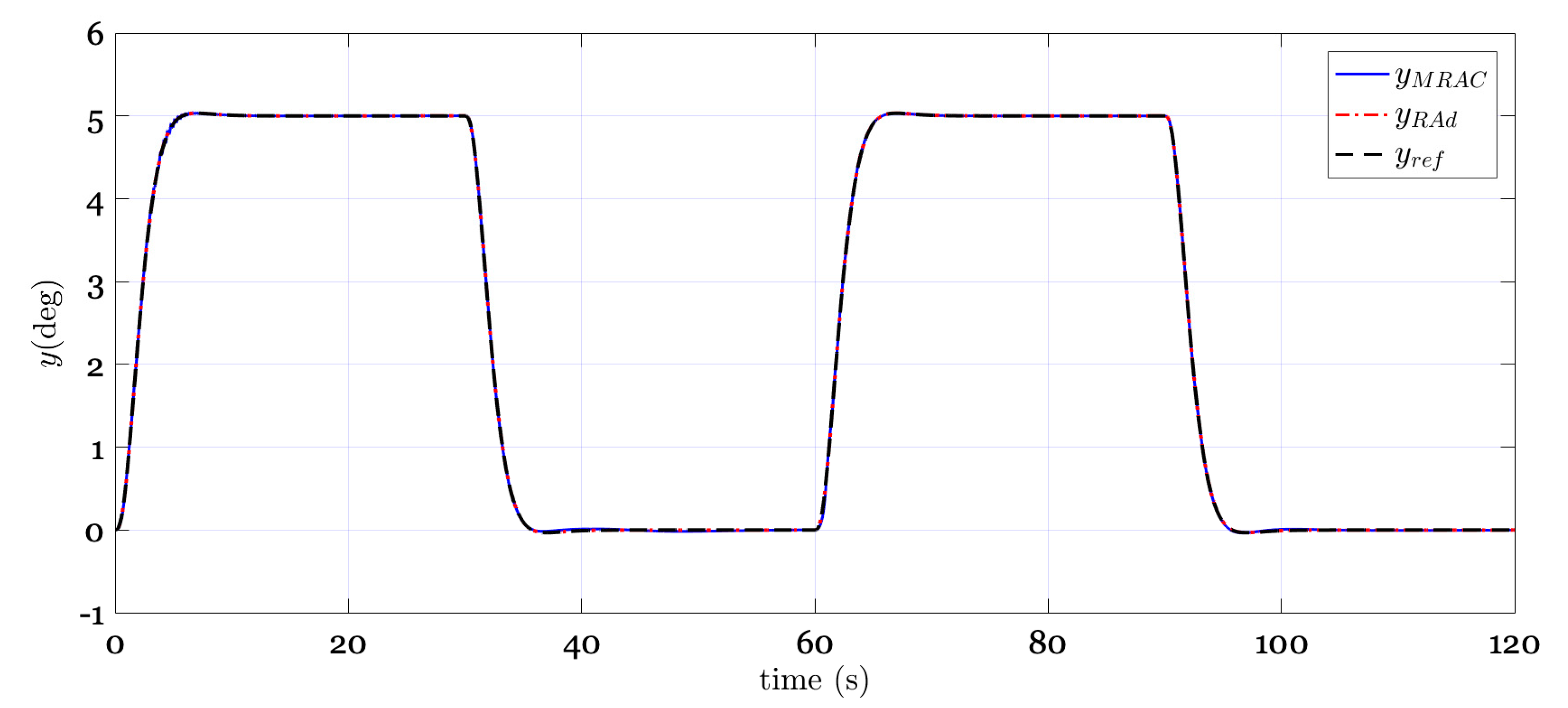
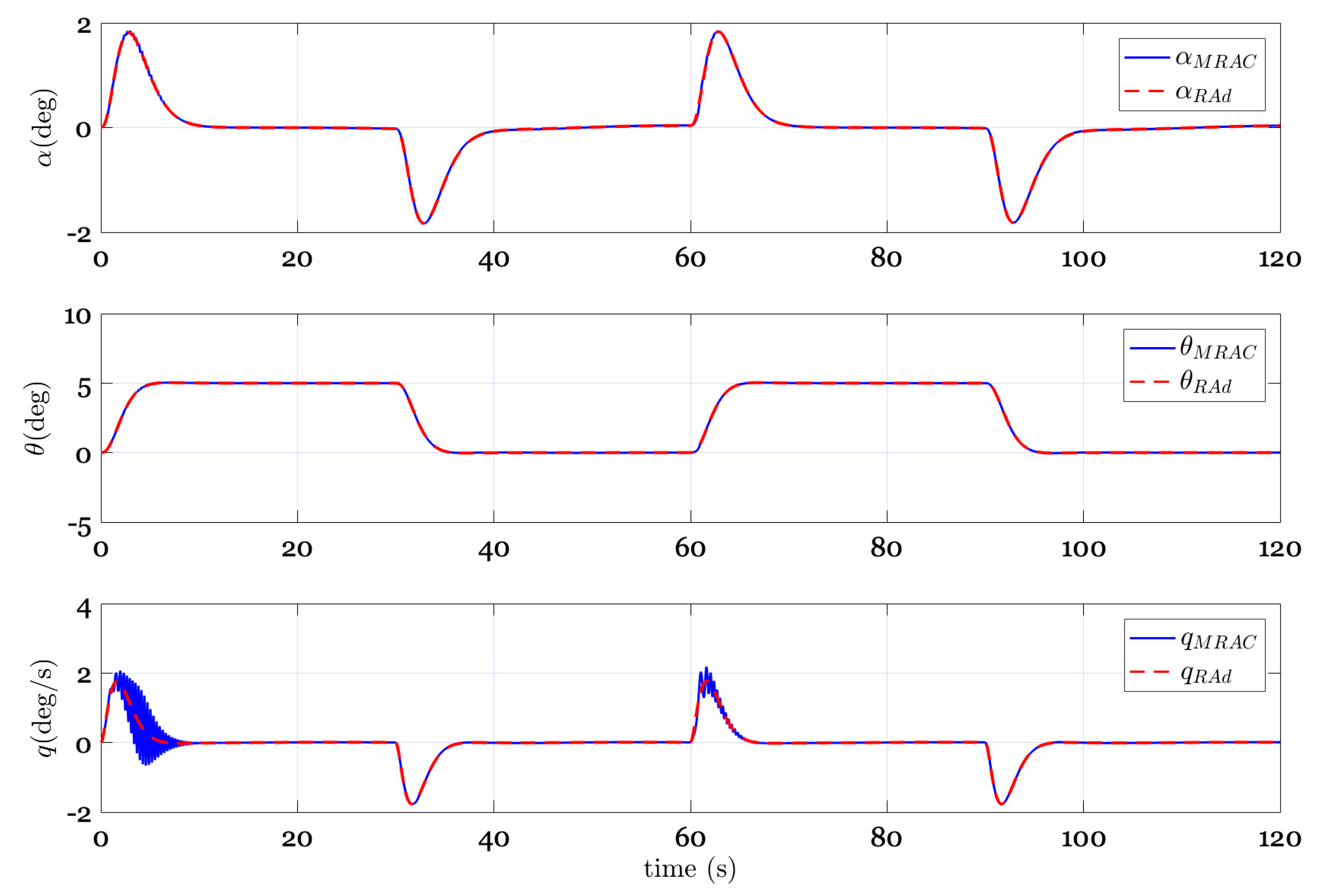
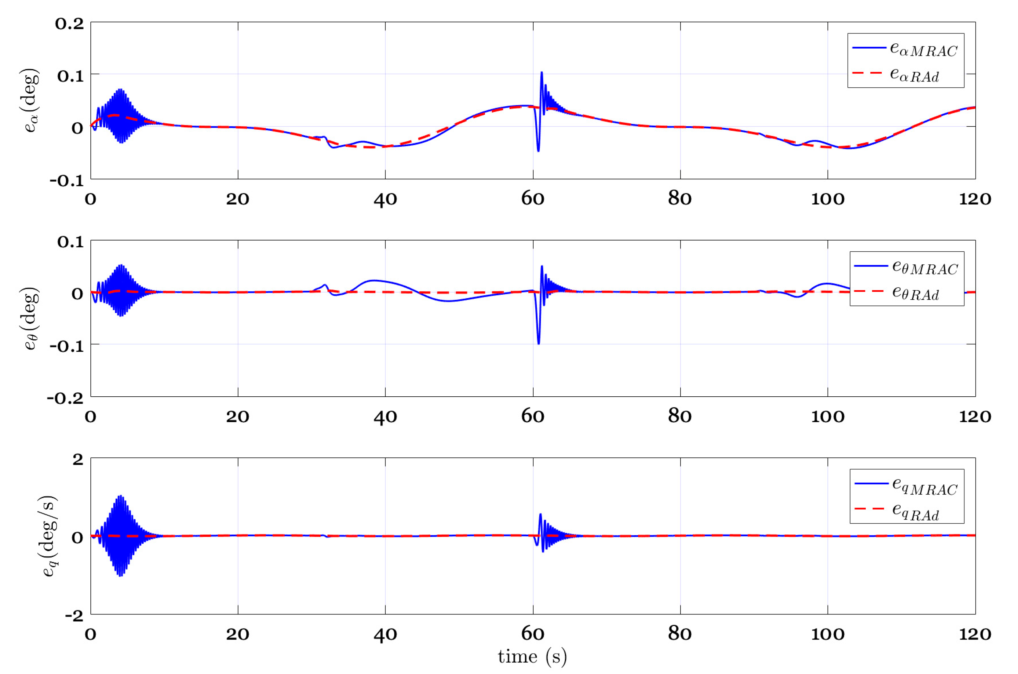
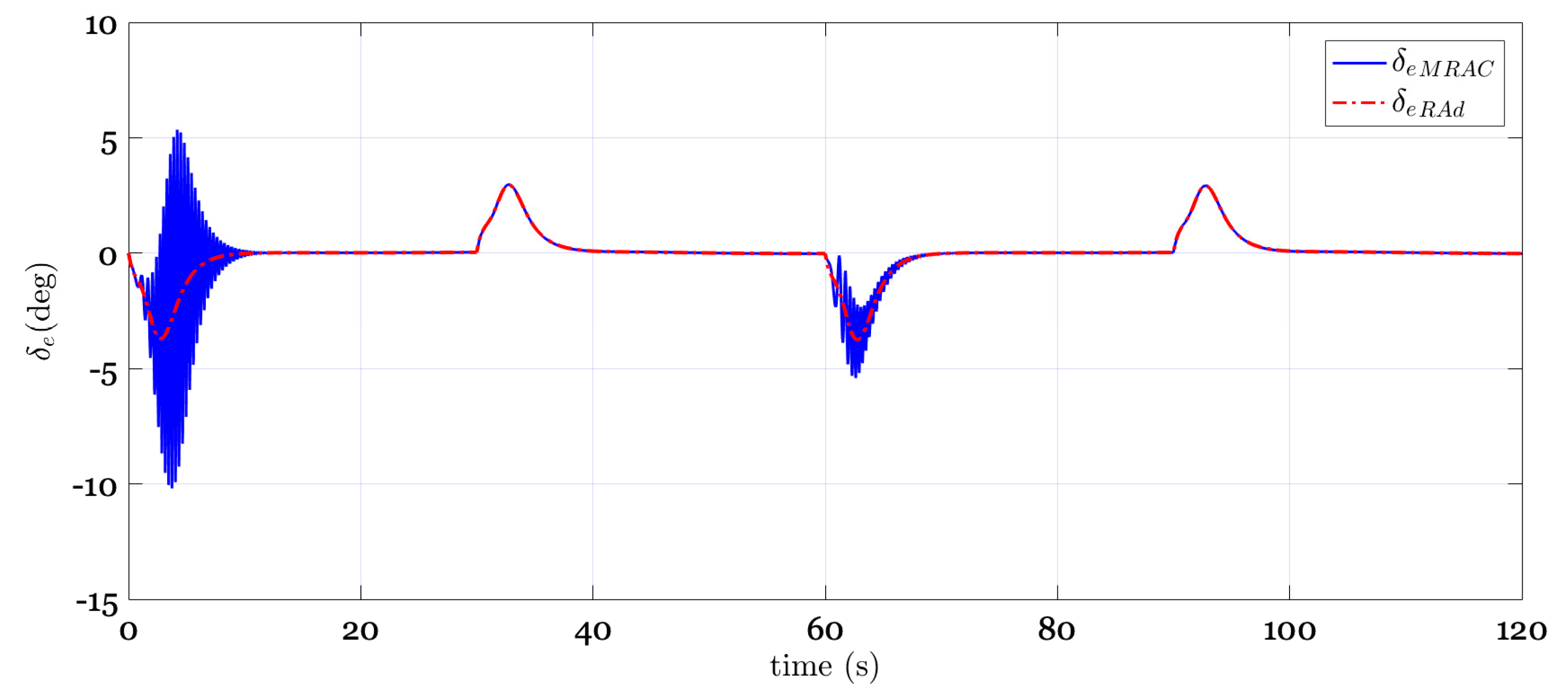
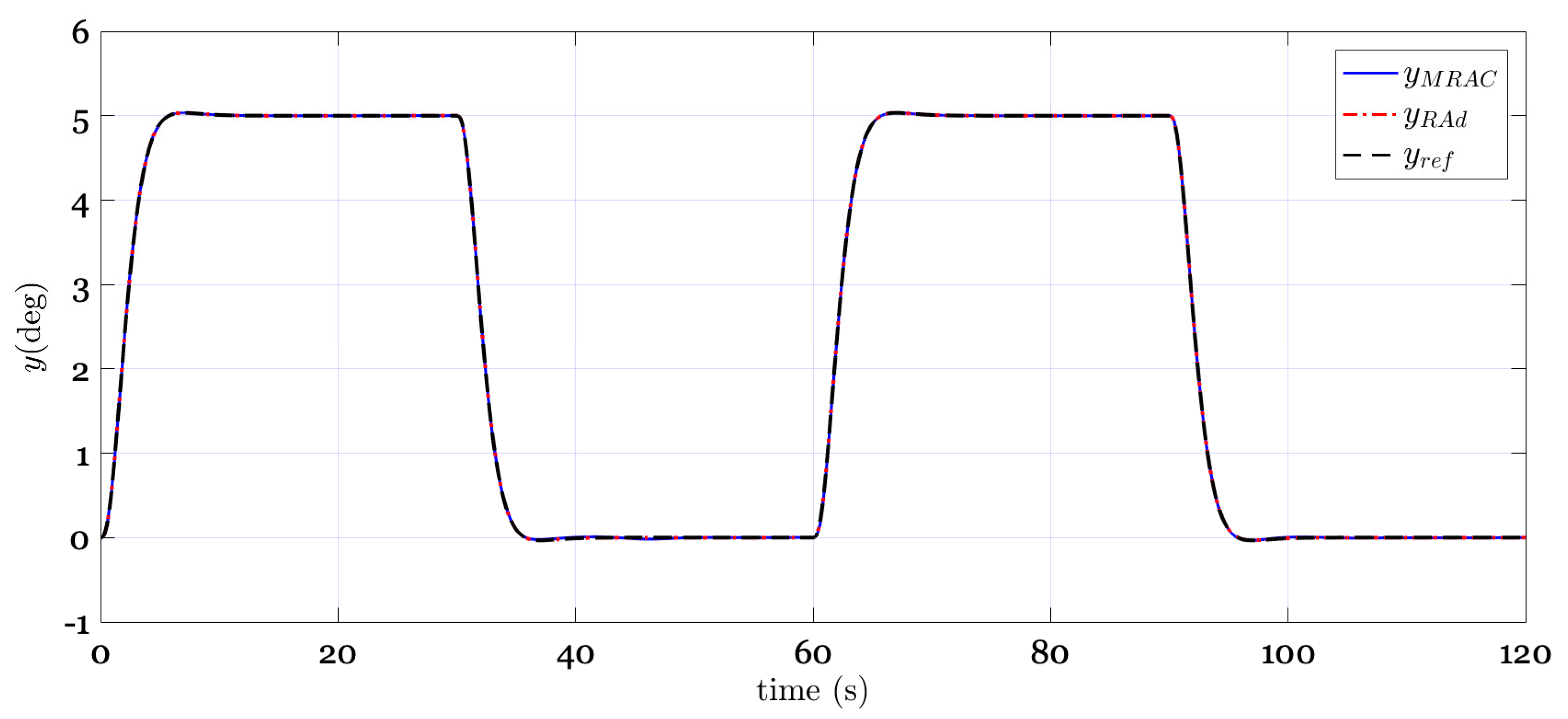
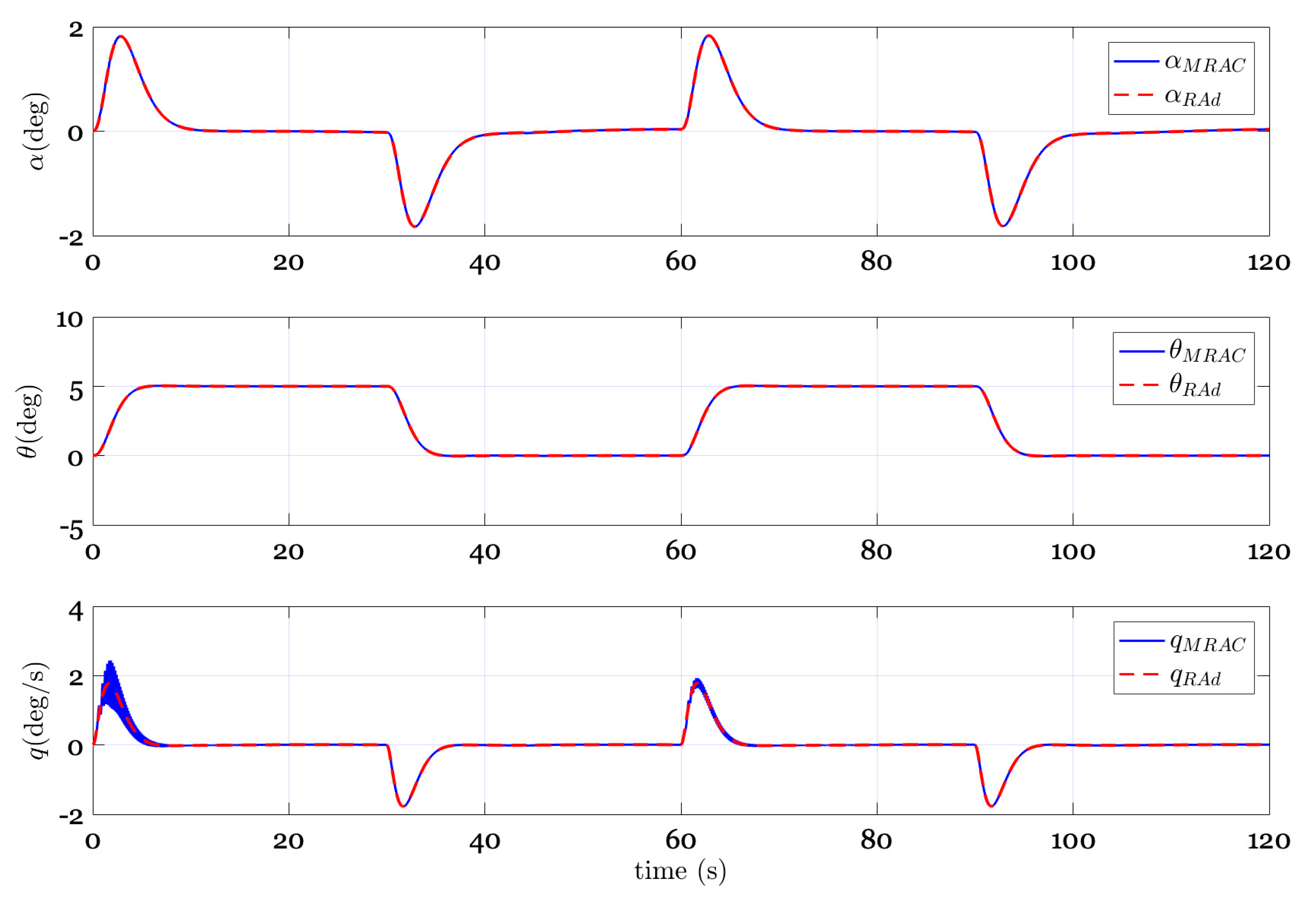
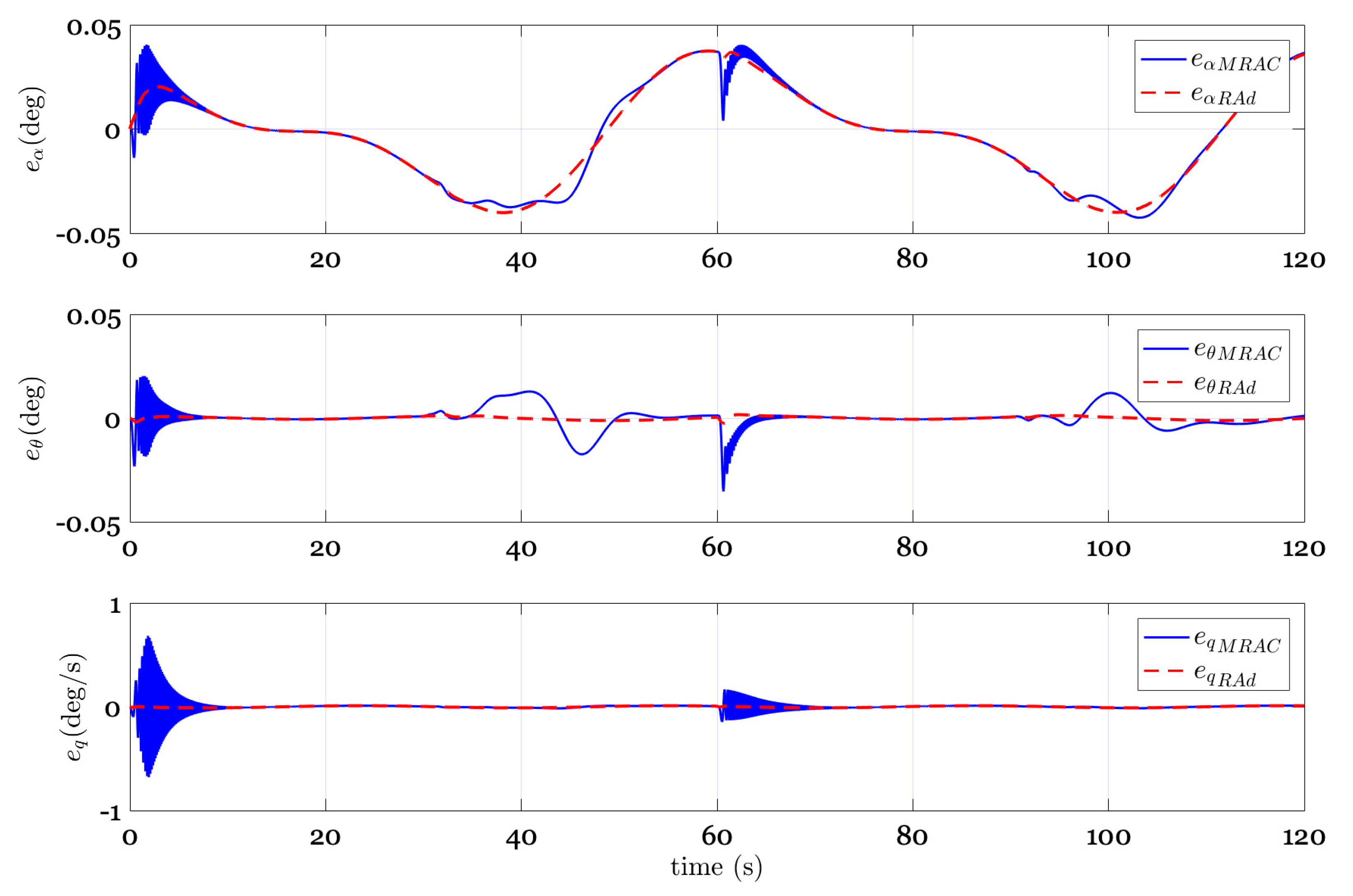
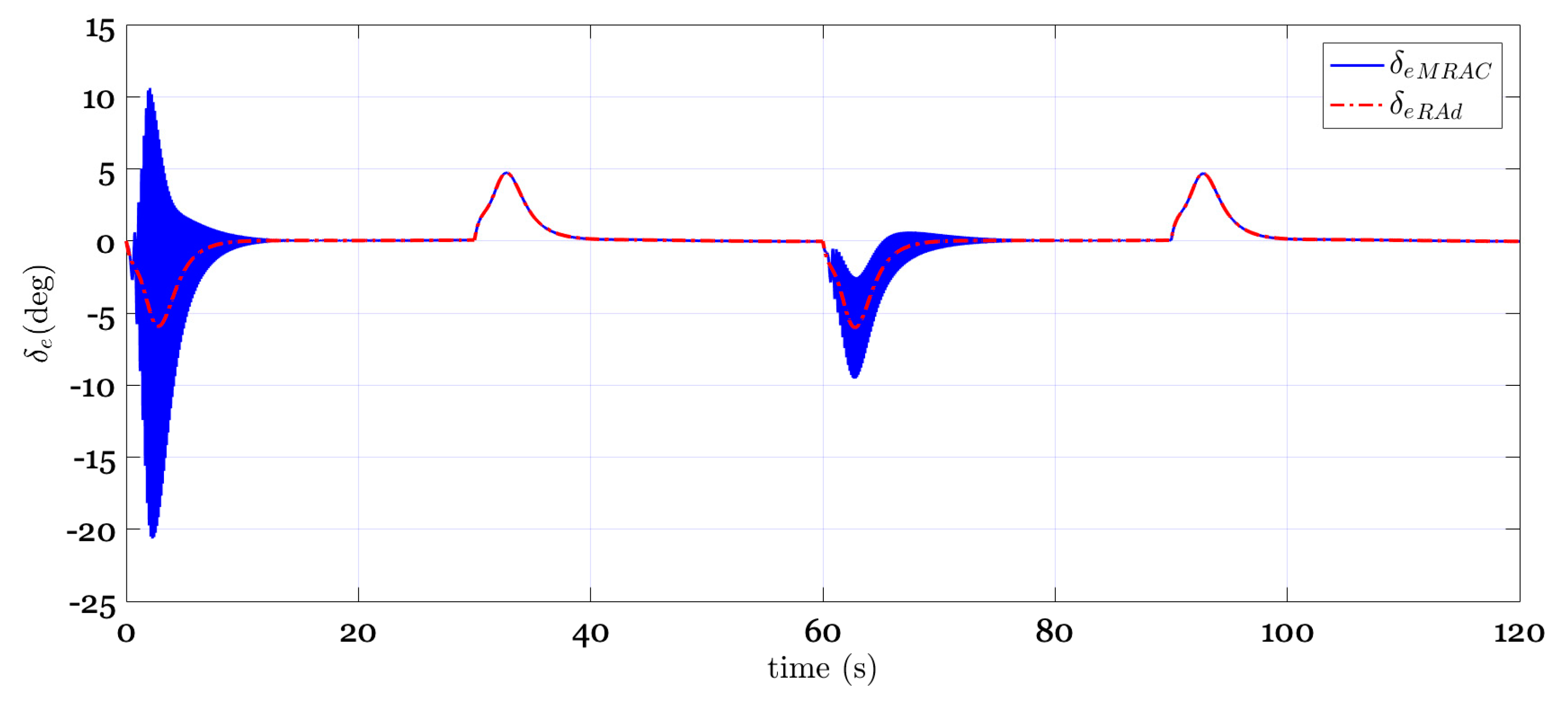
Figure 1 shows that the designed robust adaptive controller was able to achieve the expected tracking performance, while the behavior of the standard MRAC was not satisfactory when employing small adaptive gains. Figure 2 shows that the trajectories of state space performed better for the proposed control method as compared to the standard MRAC. As can be seen in Figure 3, the status errors of the standard MRAC were much higher as compared to the robust adaptive controller. The corresponding control signals shown in Figure 4 showed that the robust adaptive control responded to smooth trajectories, unlike the standard MRAC.

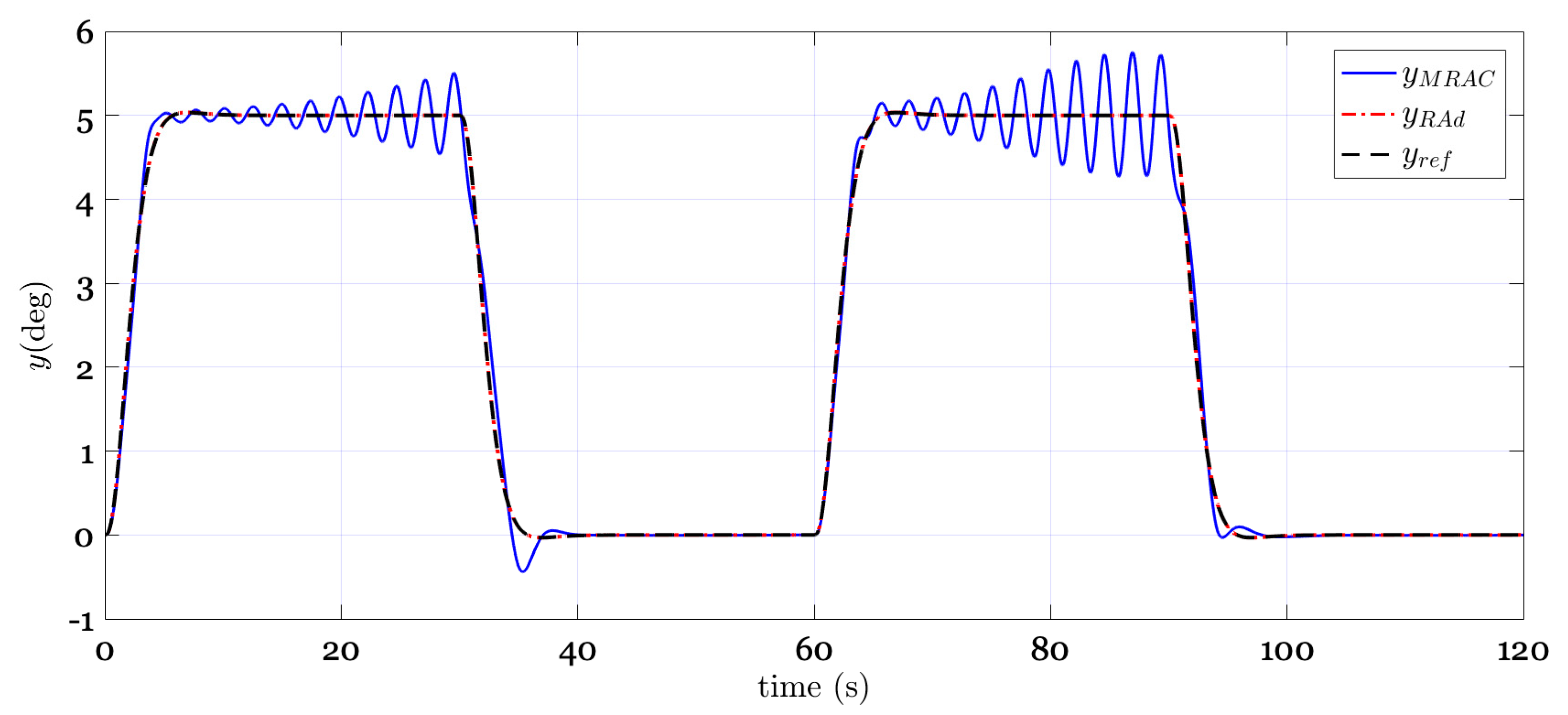
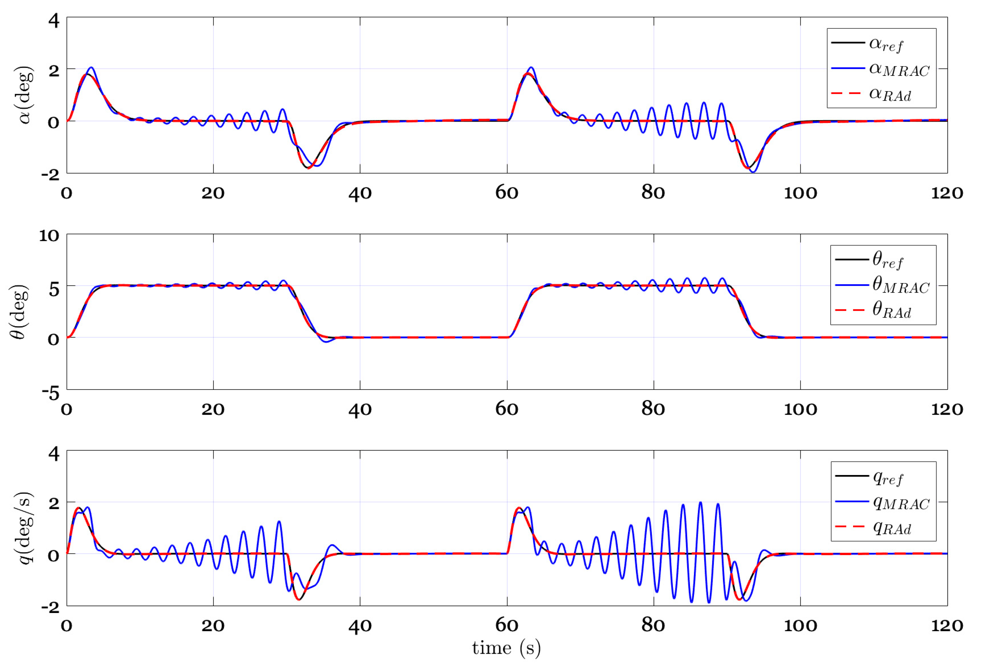
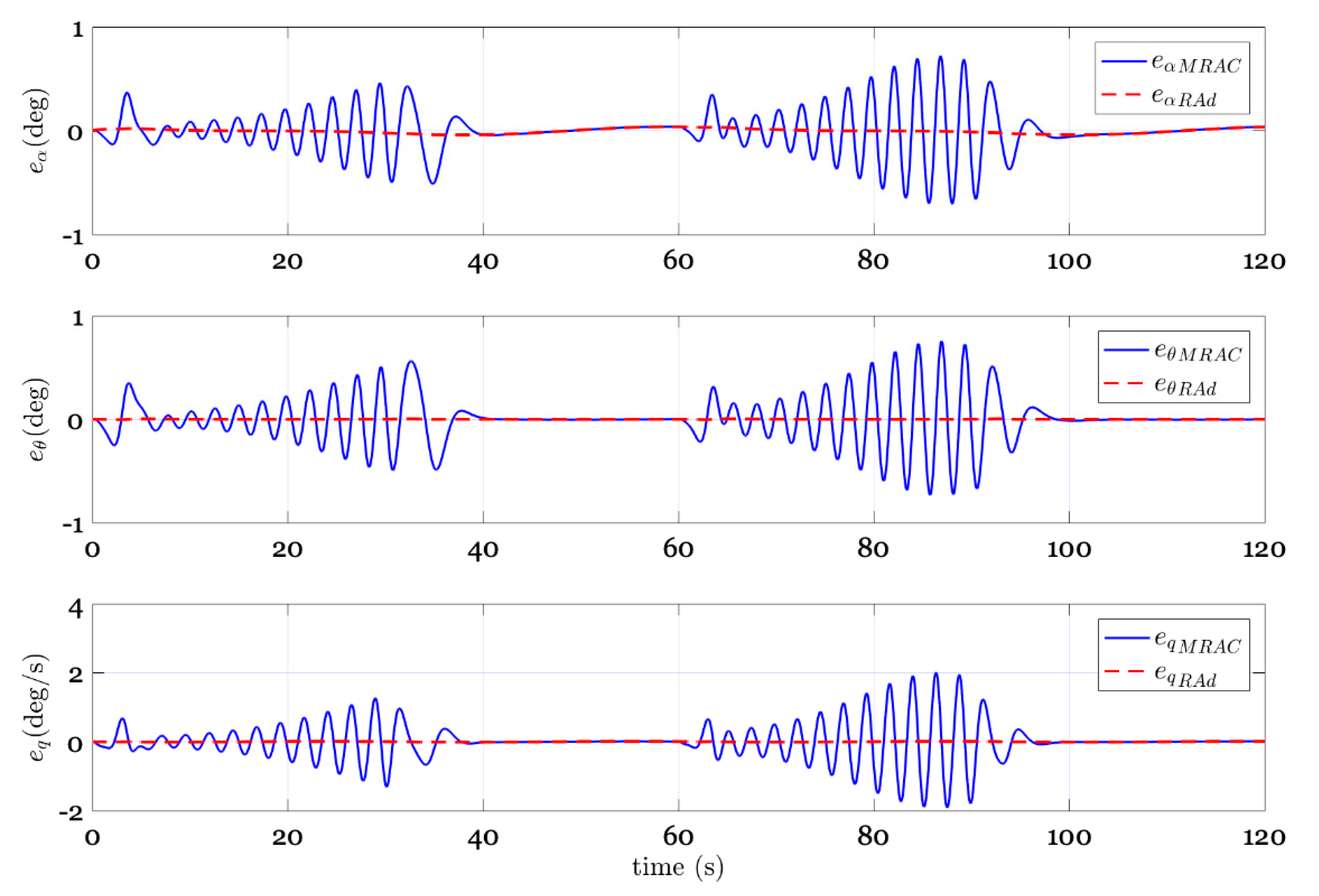
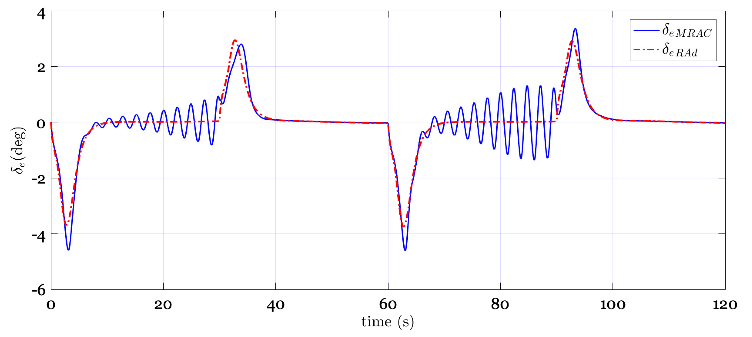
In the next simulation, to decrease tracking errors and realize fast adaptation, higher adaptive gains were selected as ${\rho }_{\lambda }={\rho }_{\theta }=1$. Figure 5 shows that the tracking performance of the standard MRAC was noticeably improved with high adaptive gains. The state trajectories and status errors displayed in Figure 6 and Figure 7 showed that the designed robust adaptive controller had superior performance. Comparing Figure 7 with Figure 3 demonstrates that increased adaptive gains effectively decreased status errors. However, Figure 8 shows that high-frequency oscillations arose in the control trajectory due to high adaptive gains for the standard MRAC, while these oscillations were eliminated by the robust adaptive controller.

Finally, we considered a severe situation where the input uncertainty corresponded to half of the nominal control effectiveness (i.e., $\mathsf{\Lambda }=0.5I$); a simulation was run by employing adaptive gains ${\rho }_{\lambda }={\rho }_{\theta }=10$ to handle the greater uncertainties.

As can be seen in Figure 9, both standard MRAC and the robust adaptive controller could track the reference command with high adaptive gains. However, the proposed robust adaptive controller performed quite well, without any high-frequency oscillations of state trajectories (Figure 10), status errors (Figure 11), or especially control signal (Figure 12), and the tracking error was further reduced to a small value. Comparing Figure 12 with Figure 8 showed that large uncertainties required a large control signal in altitude, and higher adaptation gains caused more severe high-frequency oscillations in the control response for the standard MRAC. This demonstrated that the proposed control method was robust when control effectiveness loss, uncertain dynamics, and external disturbance existed in the system.

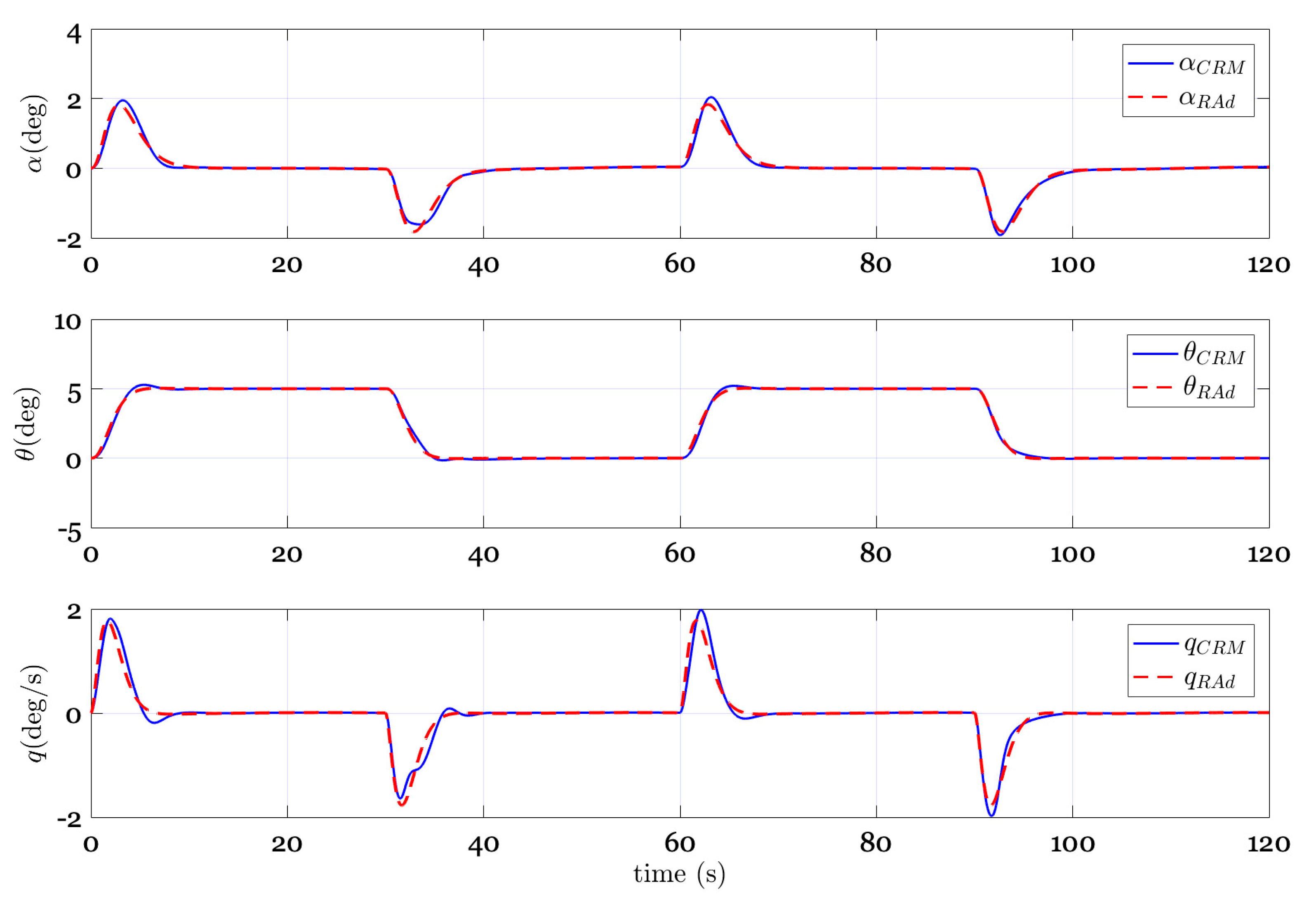
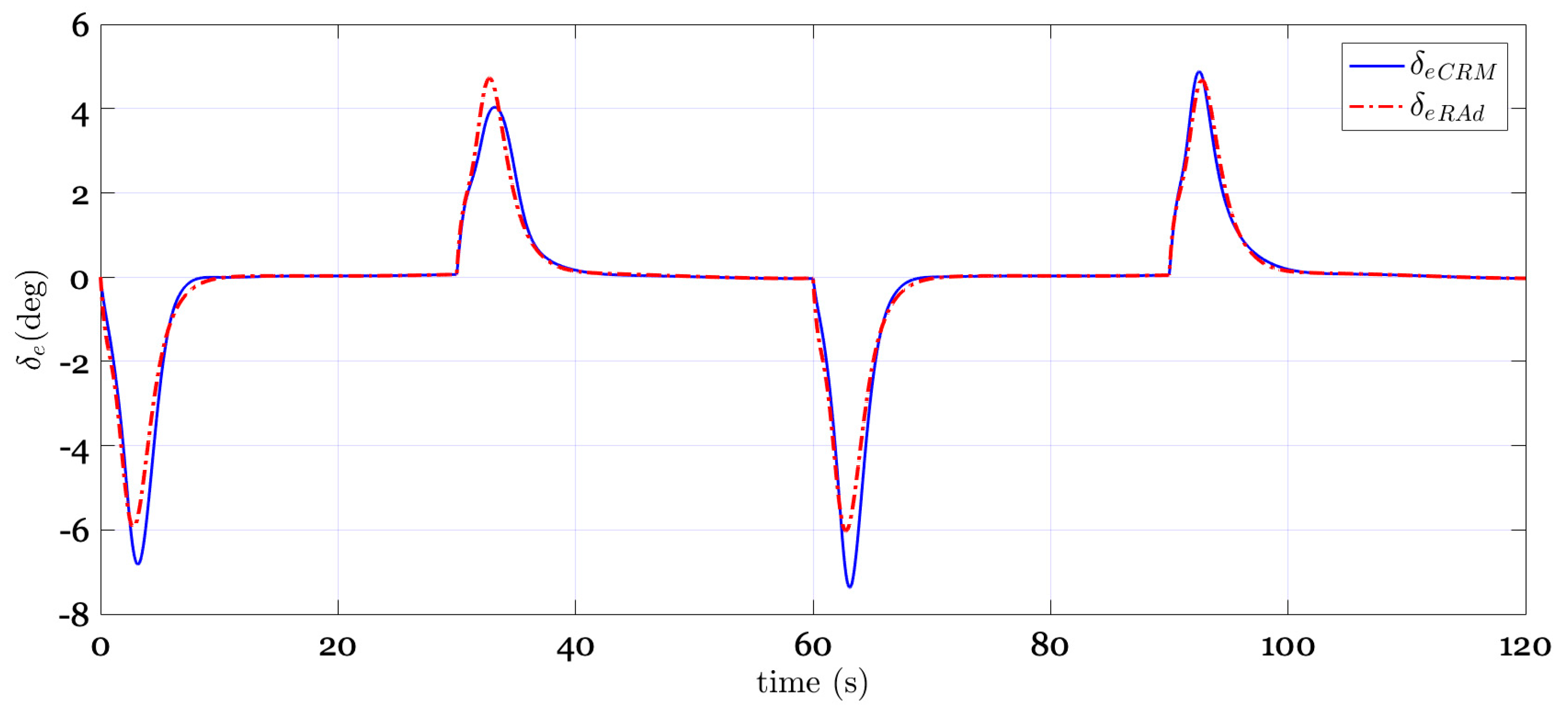
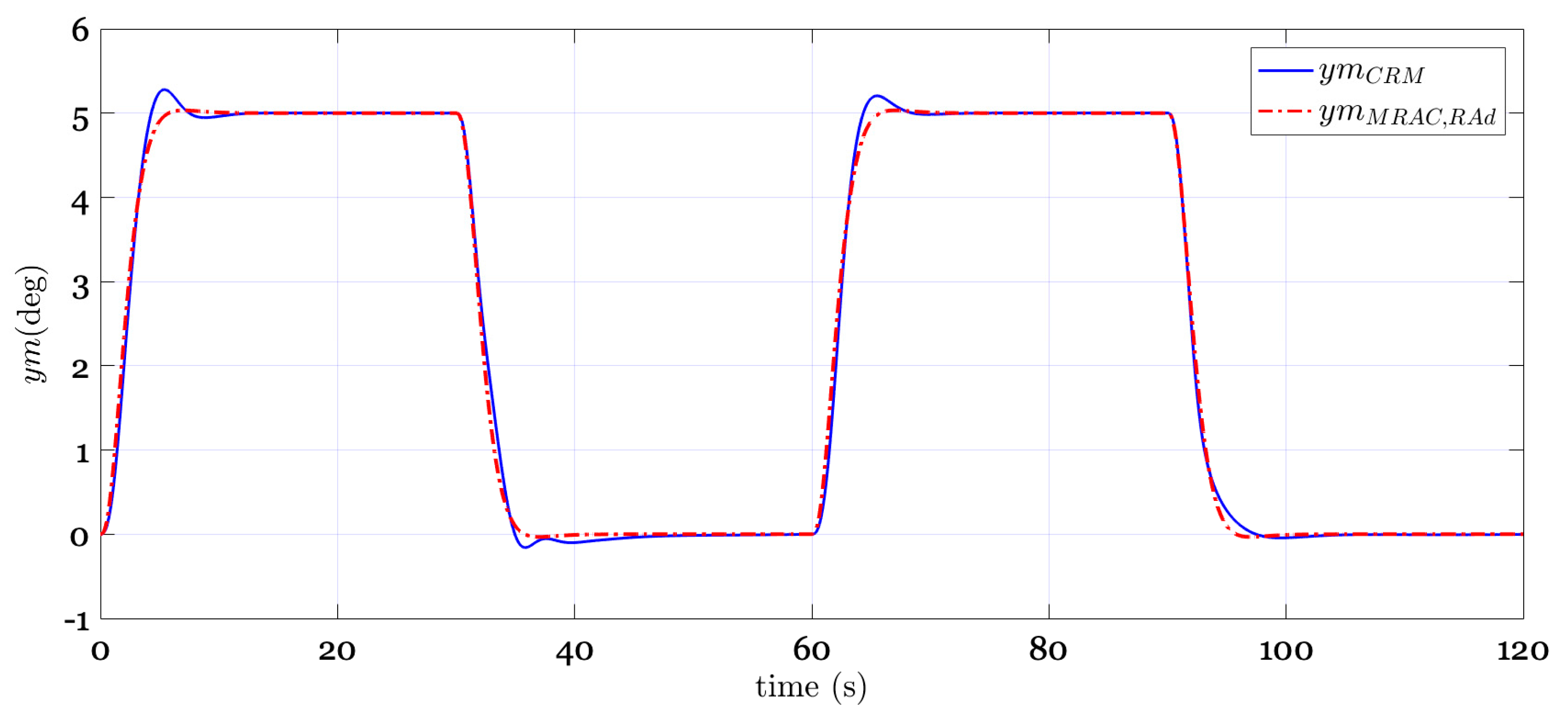
The proposed robust adaptive control was finally compared with the closed-loop reference model (CRM) adaptive control [24]. As shown in Figure 13′s state trajectories and Figure 14′s control signals, there were no high-frequency components for either CRM or the robust adaptive controller. However, as can be observed in Figure 15, the initial phase of the reference model in CRM was different from MRAC and the proposed method. These results verified that our method provides improved system transient performance that is as good as CRM, without changing the pre-designed reference model.

5. Conclusions

This paper presents a robust adaptive controller for a nonlinear aircraft system with the existence of input uncertainty, matched uncertainty, and unmatched disturbance uncertainty. The proposed control method introduced a robust compensator into the standard model reference adaptive control architecture, with the intent to resist high-frequency oscillations due to excessive adaptive gains while handling great uncertainties and pursuing fast adaptation. The robust compensator was designed using $H_{\infty }$ control theory and is intended to minimize the influence of estimate parameter errors on system responses. Simulation results demonstrated that, as compared to standard MRAC, the proposed robust adaptive controller not only guaranteed tracking performance, but also eliminated high-frequency oscillations in a control signal with fast adaptation, which ensured stability of the closed-loop system.

References

- Zong, Q.; Ji, Y.; Zeng, F.; Liu, H. Output feedback back-stepping control for a generic Hypersonic Vehicle via small-gain theorem. Aerosp. Sci. Technol. 2012, 23, 409–417. [Google Scholar] [CrossRef]
- Younes, A.B.; Turner, J.D. Derivative Enhanced Optimal Feedback Control Using Computational Differentiation. Int. J. Appl. Exp. Math. Res. Artic. 2016, 2016, 112. [Google Scholar] [CrossRef]
- Hess, R.A. Robust Flight Control Design to Minimize Aircraft Loss-of-Control Incidents. Aerospace 2014, 1, 1–17. [Google Scholar] [CrossRef] [Green Version]
- Michailidis, I.; Baldi, S.; Kosmatopoulos, E.B.; Ioannou, P.A. Adaptive Optimal Control for Large-Scale Nonlinear Systems. IEEE Trans. Autom. Control 2017, 9286, 1–11. [Google Scholar] [CrossRef] [Green Version]
- Astolfi, A.; Member, S.; Ortega, R. Immersion and Invariance: A New Tool for Stabilization and Adaptive Control of Nonlinear Systems. IEEE Trans. Automat. Control. 2003, 48, 590–606. [Google Scholar] [CrossRef] [Green Version]
- Zhang, Q.; Chen, X.; Xu, D. Adaptive Neural Fault-Tolerant Control for the Yaw Control of UAV Helicopters with Input Saturation and Full-State Constraints. Appl. Sci. 2020, 10, 1404. [Google Scholar] [CrossRef] [Green Version]
- Baek, J. Practical Adaptive Sliding-Mode Control Approach for Precise Tracking of Robot Manipulators. Appl. Sci. 2020, 10, 2909. [Google Scholar] [CrossRef] [Green Version]
- Whitaker, H.P.; Yamron, J.; Kezer, A. Design Of Model-Reference Adaptive Control Systems For Aircraft; Massachusetts Institute of Technology, Instrumentation Laboratory: Jackson & Moreland: Cambridge, MA, USA, 1958. [Google Scholar]
- Mooij, E. Numerical Investigation of Model Reference Adaptive Control for Hypersonic Aircraft. J. Guid. Control. Dyn. 2001, 24, 315–323. [Google Scholar] [CrossRef]
- Guo, J.; Tao, G.; Liu, Y. A multivariable MRAC scheme with application to a nonlinear aircraft model. Automatica 2011, 47, 804–812. [Google Scholar] [CrossRef]
- Zhao, L.; Shi, Z.; Zhu, Y. Acceleration autopilot for a guided spinning rocket via adaptive output feedback. Aerosp. Sci. Technol. 2018, 77, 573–584. [Google Scholar] [CrossRef] [Green Version]
- Ahmadi, K.; Asadi, D.; Pazooki, F. Nonlinear L1 adaptive control of an airplane with structural damage. Proc. Inst. Mech. Eng. Part G. J. Aerosp. Eng. 2019, 233, 341–353. [Google Scholar] [CrossRef]
- Lavretsky, E.; Hovakimyan, N. Stable adaptation in the presence of input constraints. Syst. Control Lett. 2007, 56, 722–729. [Google Scholar] [CrossRef]
- Rohrs, C.; Valavani, L.; Athans, M.; Stein, G. Robustness of Continuous-Time Adaptive Control Algorithms in the Presence of Unmodeled Dynamics. IEEE Trans. Autom. Control 1985, 30, 881–889. [Google Scholar] [CrossRef] [Green Version]
- Ioannout, P.A.; Kokotovic, P. V Instability Analysis and Improvement of Robustness of Adaptive Control. Automatica 1984, 20, 583–594. [Google Scholar] [CrossRef]
- Station, P.O.B.Y.; Haven, N. Improving Transient Response of Adaptive Control Systems using Multiple Models and Switching. IEEE Trans. Autom. Control 1994, 39, 1861–1866. [Google Scholar] [CrossRef]
- Manuel, A.; Duarte, K.S.N. Combined Direct and Indirect Approach to Adaptive Control. IEEE Trans. Autom. Control 1989, 34, 1071–1075. [Google Scholar] [CrossRef]
- Lavretsky, E. Combined/Composite Model Reference Adaptive Control. IEEE Trans. Autom. Control 2009, 54, 2692–2697. [Google Scholar] [CrossRef]
- Gregory, I.M.; Gadient, R.O.; Lavretsky, E. Flight Test of Composite Model Reference Adaptive Control (CMRAC) Augmentation Using NASA AirSTAR Infrastructure. AIAA Guid. Navig. Control Conf. 2011, 2011, 6452. [Google Scholar] [CrossRef] [Green Version]
- Cao, C.; Hovakimyan, N. Design and Analysis of a Novel L1 Adaptive Control Architecture With Guaranteed Transient Performance. IEEE Trans. Autom. Control 2008, 53, 586–591. [Google Scholar] [CrossRef]
- Gregory, I.; Xargay, E.; Cao, C.; Hovakimyan, N. L1 Adaptive Control Design for NASA AirSTAR Flight Test Vehicle. AIAA Guid. Navig. Control Conf. 2009, 1–27. [Google Scholar] [CrossRef]
- Yucelen, T.; Haddad, W.M. Low-Frequency Learning and Fast Adaptation in Model Reference Adaptive Control. IEEE Trans. Autom. Control 2013, 58, 1080–1085. [Google Scholar] [CrossRef]
- Rajpurohit, T.; Haddad, W.M.; Yucelen, T. Output Feedback Adaptive Control with Low-Frequency Learning and Fast Adaptation. J. Guid. Control Dyn. 2016, 39, 16–31. [Google Scholar] [CrossRef] [Green Version]
- Gibson, T.E.; Qu, Z.; Anuradha, M.A.; Lavretsky, E. Adaptive output feedback based on closed-loop reference models. IEEE Trans. Automat. Contr. 2015, 60, 2728–2733. [Google Scholar] [CrossRef] [Green Version]
- Lavretsky, E.; Wise, K.A. Robust and Adaptive Control with Aerospace Applications; Advanced Textbooks in Control and Signal Processing; Springer: London, UK, 2013; ISBN 978-1-4471-4395-6. [Google Scholar]
- Qu, Z.; Annaswamy, A.M. Adaptive output-feedback control with closed-loop reference models for very flexible aircraft. J. Guid. Control Dyn. 2016, 39, 873–888. [Google Scholar] [CrossRef]
- Wiese, D.P.; Annaswamy, A.M.; Muse, J.A.; Bolender, M.A.; Lavretsky, E. Adaptive output feedback based on closed-loop reference models for hypersonic vehicles. J. Guid. Control Dyn. 2015, 38, 2429–2440. [Google Scholar] [CrossRef] [Green Version]
- Xie, L.; Minyue, F.; de Souza, C. E H∞ control and quadratic stabilization of systems with parameter uncertainty via output feedback. IEEE Trans. Autom. Control 1992, 37, 1253–1256. [Google Scholar] [CrossRef]
- Scherer, C. The Riccati Inequality and State-Space H∞ Optimal Control; Diss. Julius Maximilians University: Würzburg, Germany, 1990. [Google Scholar]
- Nguyen, N.; Field, M. Least-Squares Model-Reference Adaptive Control with Chebyshev. J. Aerosp. Inf. Syst. 2013, 10, 29–31. [Google Scholar] [CrossRef]
Figure 1.
Tracking performance for model reference adaptive control (MRAC) and robust adaptive controller with .
Figure 2.
Aircraft response for MRAC and robust adaptive controller with .
Figure 3.
Status errors from MRAC and robust adaptive controller with .
Figure 4.
Control signal from MRAC and robust adaptive controller with .
Figure 5.
Tracking performance for MRAC and robust adaptive controller with .
Figure 6.
Figure 7.
Figure 8.
Figure 9.
Figure 10.
Figure 11.
Figure 12.
Figure 13.
Aircraft response for closed-loop reference model (CRM) and robust adaptive controller with .
Figure 14.
Control signal from CRM and robust adaptive controller with .
Figure 15.
Reference model from CRM and robust adaptive controller with .
© 2020 by the authors. Licensee MDPI, Basel, Switzerland. This article is an open access article distributed under the terms and conditions of the Creative Commons Attribution (CC BY) license (http://creativecommons.org/licenses/by/4.0/).
Share and Cite
MDPI and ACS Style
Chen, J.; Wang, J.; Wang, W. Robust Adaptive Control for Nonlinear Aircraft System with Uncertainties. Appl. Sci. 2020, 10, 4270. https://doi.org/10.3390/app10124270
AMA Style
Chen J, Wang J, Wang W. Robust Adaptive Control for Nonlinear Aircraft System with Uncertainties. Applied Sciences. 2020; 10(12):4270. https://doi.org/10.3390/app10124270
Chicago/Turabian StyleChen, Jiao, Jiangyun Wang, and Weihong Wang. 2020. "Robust Adaptive Control for Nonlinear Aircraft System with Uncertainties" Applied Sciences 10, no. 12: 4270. https://doi.org/10.3390/app10124270
Note that from the first issue of 2016, this journal uses article numbers instead of page numbers. See further details here.