Prediction of Pile Axial Bearing Capacity Using Artificial Neural Network and Random Forest
by
 , , ,
, , ,
Tuan Anh Pham
* ,
,
Hai-Bang Ly
* ,
,
Van Quan Tran
,
Loi Van Giap
,
Huong-Lan Thi Vu
and
Hong-Anh Thi Duong
University of Transport Technology, Hanoi 100000, Vietnam
*
Authors to whom correspondence should be addressed.
Appl. Sci. 2020, 10(5), 1871; https://doi.org/10.3390/app10051871
Submission received: 5 January 2020
/
Revised: 3 March 2020
/
Accepted: 5 March 2020
/
Published: 9 March 2020
(This article belongs to the Special Issue Soft Computing Techniques in Structural Engineering and Materials)
Abstract
:Axial bearing capacity of piles is the most important parameter in pile foundation design. In this paper, artificial neural network (ANN) and random forest (RF) algorithms were utilized to predict the ultimate axial bearing capacity of driven piles. An unprecedented database containing 2314 driven pile static load test reports were gathered, including the pile diameter, length of pile segments, natural ground elevation, pile top elevation, guide pile segment stop driving elevation, pile tip elevation, average standard penetration test (SPT) value along the embedded length of pile, and average SPT blow counts at the tip of pile as input variables, whereas the ultimate load on pile top was considered as output variable. The dataset was divided into the training (70%) and testing (30%) parts for the construction and validation phases, respectively. Various error criteria, namely mean absolute error (MAE), root mean squared error (RMSE), and the coefficient of determination (R2) were used to evaluate the performance of RF and ANN algorithms. In addition, the predicted results of pile load tests were compared with five empirical equations derived from the literature and with classical multi-variable regression. The results showed that RF outperformed ANN and other methods. Sensitivity analysis was conducted to reveal that the average SPT value and pile tip elevation were the most important factors in predicting the axial bearing capacity of piles.
1. Introduction
In applied engineering, piles have been used as the foundation elements, in which the axial bearing capacity of the pile (Pu) is considered as the most important parameter in the design of pile foundation. Normally, the axial bearing capacity of piles can be determined by five approaches, namely the static analysis, dynamic analysis, dynamic testing, pile load testing, and in-situ testing [1]. Out of these methods, the pile load test is considered as the best method to determine the pile bearing capacity. However, such a method is time-consuming, and the costs are often difficult to justify for ordinary or small projects, whereas other methods have lower accuracy. As a result, several approaches have been developed to predict the axial bearing capacity of pile or to enhance the prediction accuracy. The nature of these methods included some simplifications, assumptions, or empirical approaches with respect to the soil stratigraphy, soil–pile structure interactions, and the distribution of soil resistance along the pile. In such studies, the test results were used as complementary elements to improve the prediction accuracy. Meanwhile, the European standard (Euro code 7) [2] recommends using the following ground field tests: DP (dynamic probing test), SS (press-in and screw-on probe test), SPT (standard penetration test), PMT (pressure meter tests), PLT (plate loading test), DMT (flat dilatometer test), FVT (field vane test), CPTu (cone penetration tests with the measurement of pore pressure). Among the above indicators, the SPT is commonly used to determine the bearing capacity of piles [3]. Several propositions relying on the results of SPT have been proposed to predict the bearing capacity of piles, including the empirical equations derived from the works of Meyerhof [4], Bazaraa and Kurkur [5], Robert [6], Shioi and Fukui [7], Shariatmadari et al. [8]. In general, the pile diameter, SPT blow counts along the pile shaft, and at the tip of the pile have been used in these equations. Besides, Lopes and Laprovitera [9] proposed a formula to estimate the pile bearing capacity for different types of soil, namely sand, and silt. Decort [10] has presented an empirical formula, including the adjustment factors for sandy and clay soils. Last but not least, the Architectural Institute of Japan (AIJ) [11] has a recommendation using an experimental formula, taking into account the effects of soil type or the use of SPT value for sandy soil and untrained shear strength of soil (Cu) for clayey soil. Overall, traditional methods or empirical equations attempted to include a few key parameters to predict the pile strength. However, if the input parameters of pile geometry and soil properties increased, these methods were impossible to use.
In recent years, a widespread development in the use of information technology in civil engineering has paved the way for many promising applications, especially the use of machine learning (ML) approaches to solve practical engineering problems [12,13,14,15,16,17,18,19,20,21]. Moreover, different ML techniques have been used, for instance, decision tree [22], hybrid artificial intelligence approaches [23,24,25], artificial neural network (ANN) [26,27,28,29,30,31], adaptive neuro-fuzzy inference system (ANFIS) [32,33], and support vector machine (SVM) [34] in solving many real-world problems, including the prediction of behavior of piles. Precisely, Kumar et al. [35] developed a K-nearest neighbors (KNN) model to estimate the soil parameters required for foundation design. In another work, Goh et al. [36,37] presented an ANN model to predict the friction capacity of driven piles in clays, which was trained by on-field data records. Besides, Shahin et al. [38,39,40,41] developed an ANN model for driven piles and drilled shafts using a series of in-situ load tests as well as CTP results. Nawari et al. [42] developed an ANN algorithm to predict the deflection of drilled shafts based on SPT data and the shaft geometry. In addition, Pooya et al. [43] developed a model to predict the pile settlement using ANN, based on SPT data using 12 input factors. Last but not least, Momeni et al. [44] presented an ANN model to predict the shaft and tip resistance of concrete piles. In general, ML algorithm could be considered as an efficient tool for predicting the mechanical behavior of piles. However, no general argument has yet been reached on the selection of the best model to predict the bearing capacity of piles. Moreover, the database is an important factor that highly affects the accuracy of ML algorithms and crucial to provide a reliable modeling tool. The existing database in the literature related to the bearing capacity problem was still limited due to the lack of experiments or on-field measurements.
Therefore, the main objective of this study is dedicated to investigating the prediction capability of ANN and random forest (RF) algorithms, using all possible factors that might affect the bearing capacity of driven piles. To this aim, a considerable effort in collecting 2314 pile load test reports from the construction site of Ha Nam—Vietnam was devoted, which, to the best of our knowledge, is the largest database in the available literature. The database was then divided into the training and testing subsets, dedicated to the learning and validation phases of the two proposed ML models. Various error criteria—namely, the mean absolute error (MAE), root mean squared error (RMSE), and the coefficient of determination (R2)—were applied to evaluate the prediction capability of the algorithms. In addition, 1000 simulations taking into account the random splitting of the dataset were conducted for each model in order to finely evaluate the accuracy of RF and ANN. Proved to outperform ANN, the RF algorithm was next used to compare with five empirical formulas in the literature as well as classical multivariable regression (MVR) in predicting the bearing capacity of piles. Finally, the feature importance analysis was proposed to find out the important factors affecting the prediction capability of the RF model.
2. Significance of the Research Study
Accurately predicting the axial bearing capacity of pile is of crucial importance because of many possible advantages and contributions to foundation engineering. Numerical or experimental approaches in the available literature still face some limitations, for instance, the lack of dataset samples (Momeni et al. [44] with 36 samples; Bagińska and Srokosz [45] with 50 samples; Teh et al. [46] with 37 samples), accuracy assessment and improvement of the ML algorithms or comparison with classical prediction methodologies. Therefore, the contribution of the present work could be highlighted through the following ideas: (i) the largest dataset, to the best of the author’s knowledge, was used for the construction of ML models, including 2314 experimental tests; (ii) a comparison of two ML algorithms, namely ANN and RF, was conducted and compared with classical MVR and five formulas in the literature to fully assess the prediction performance of each approach; (iii) the performance of ML algorithms was evaluated under the presence of random splitting dataset, which could truly find out the efficiency of ML algorithms; and (iv) a sensitivity analysis was performed to reveal the role of each input parameters in predicting the axial bearing capacity of piles.
3. Data Collection and Preparation
3.1. Experimental Measurement of Bearing Capacity
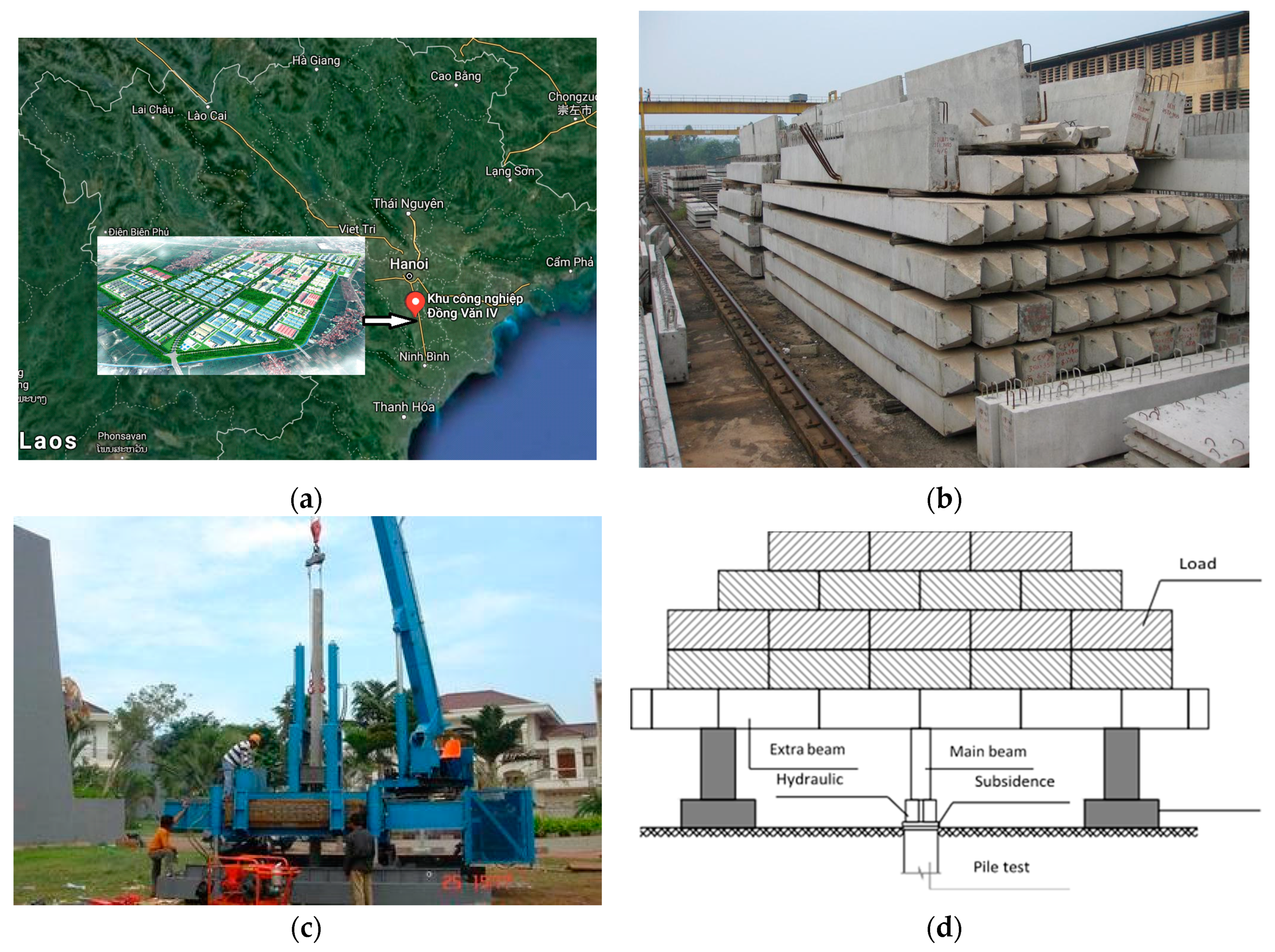
In this work, pile load tests were conducted on 2314 reinforced concrete piles at the test site in Ha Nam province—Vietnam, where the location is shown in Figure 1a. Pre-cast square section piles with closed tips were driven to the ground by hydraulic pile presses machine with a constant rate of penetration. The piles were assembled from 1 to 3 pile segments, connected by welding through intermediate steel plates and fixed steel plates at the top of each pile segment. The pile top was driven into the ground to the pile top elevation design by the use of the guide pile segment. These pile load tests started at least 7 days after piles were driven, and the experimental layout could be depicted in Figure 1b–d. In each pile test, the load increased progressively. If, after one hour of monitoring, the settlement of the pile top was less than 0.20 mm, the load was increased to a new level. Depending on the design requirements, piles could load up to 200% of the design load. The time required for 100%, 150%, and 200% of load could last for more than 6 h to 12 h or 24 h, respectively. The determination of the bearing capacity of piles were conducted as follows:
- (i)
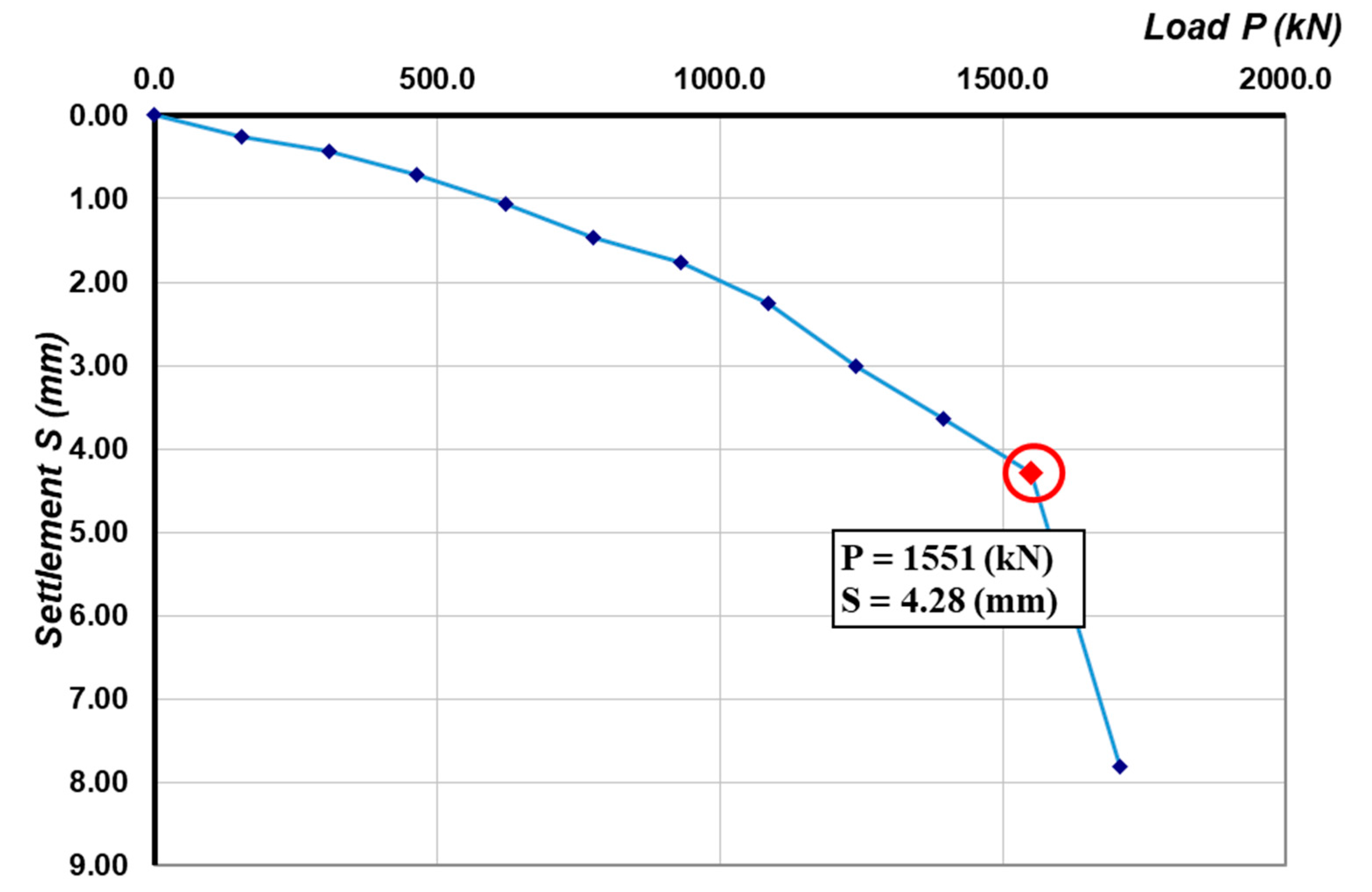
- (i) If the settlement of pile top at a given load level was 5 times higher than the settlement of pile top at the previous load level, or the settlement of the pile top at a given load level increased continuously while the load did not increase, the pile bearing capacity was determined based on that given failure load. The number of piles corresponded to this situation was 688, representing about 30% of the samples. An example of this situation is given in Appendix A (Figure A1).
- (ii)
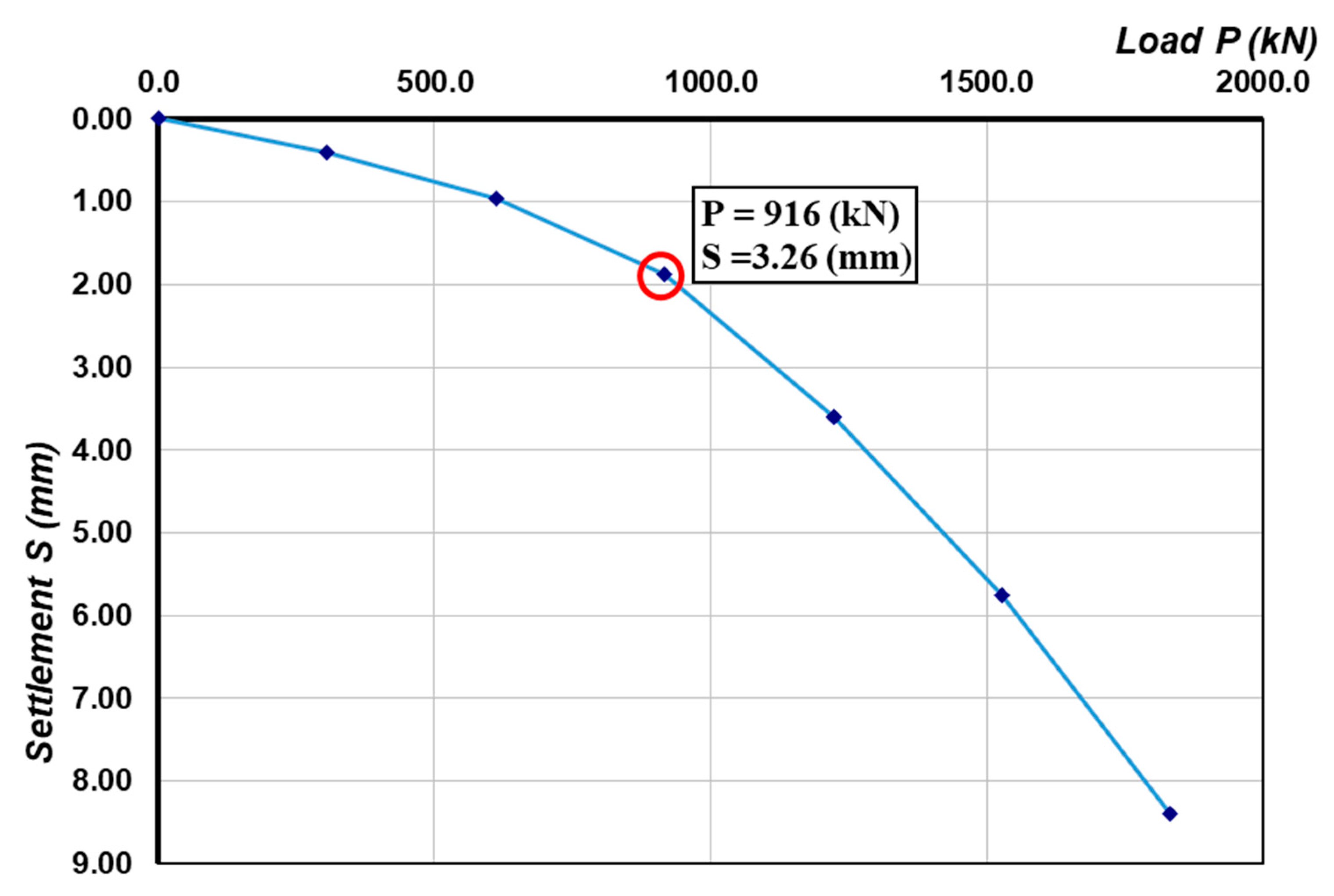
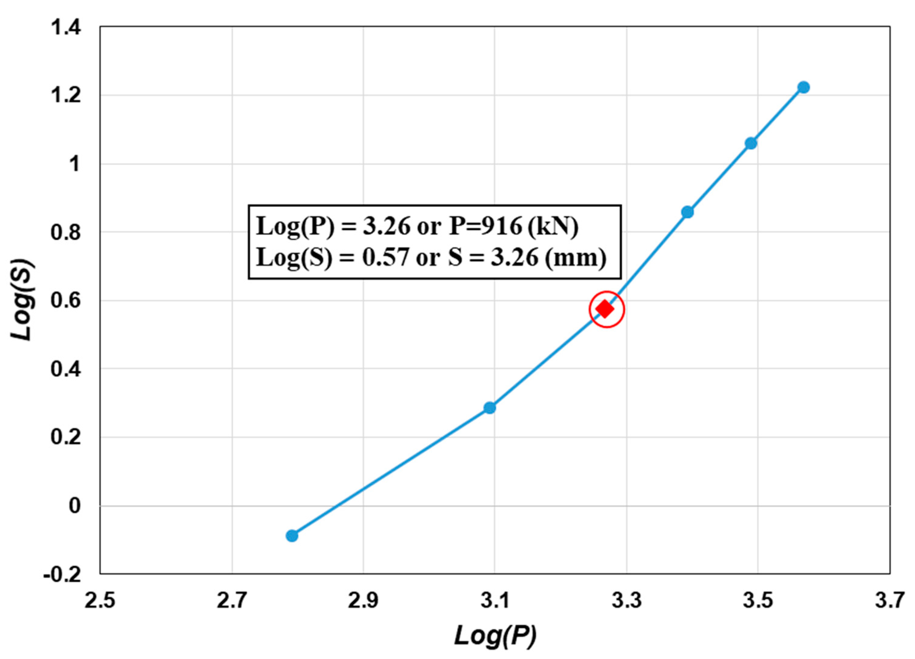
- When the pile load capacity was too large to be able to test by the destructive load, the load curve (P)– settlement (S) was plotted in log(P)–log(S). The intersection point of two lines was considered as a result of failure and taken as the pile bearing capacity, according to De Beer (1968) [47]. The number of piles corresponded to this situation was 1225 piles (accounting for more than 50% of the samples). An example of this situation is given in Appendix A (Figure A2 and Figure A3).
- (iii)
- For the remaining samples, when the log(P)–log(S) relationship is linear, which could not find the intersection point compared with the previous case. The determination of the pile bearing capacity was taken at the load level when the settlement of the pile top exceeded 10% of the pile diameter.
3.2. Data Preparation
In order to correctly predict the bearing capacity of piles, a thorough understanding of the factors that affect the bearing capacity of the pile is needed. Most traditional pile bearing capacity determination methods included the following parameters: pile geometry, pile material properties, and soil properties [4,5]. The depth of the water table was not included in this study, as it is believed that the effect is already accounted in the SPT blow counts [43]. Since the bearing capacity of piles depended on the soil compressibility and the SPT was one of the most commonly used tests in practice (indicating the in situ compressibility of soils), the SPT blow count/300 mm (N) along the embedded length of the pile was used as a measure of soil compressibility. In this study, the average SPT blow count along the pile shaft (Ns) and pile tip (Nt) were calculated. It is worth mentioning that, in order to obtain the average SPT (Nt) value around the pile tip, Meyerhof’s recommendation (1976) [4] was considered. The average SPT (Nt) value for 8D above and 3D below the pile tip was obtained, where D represented the pile diameter.
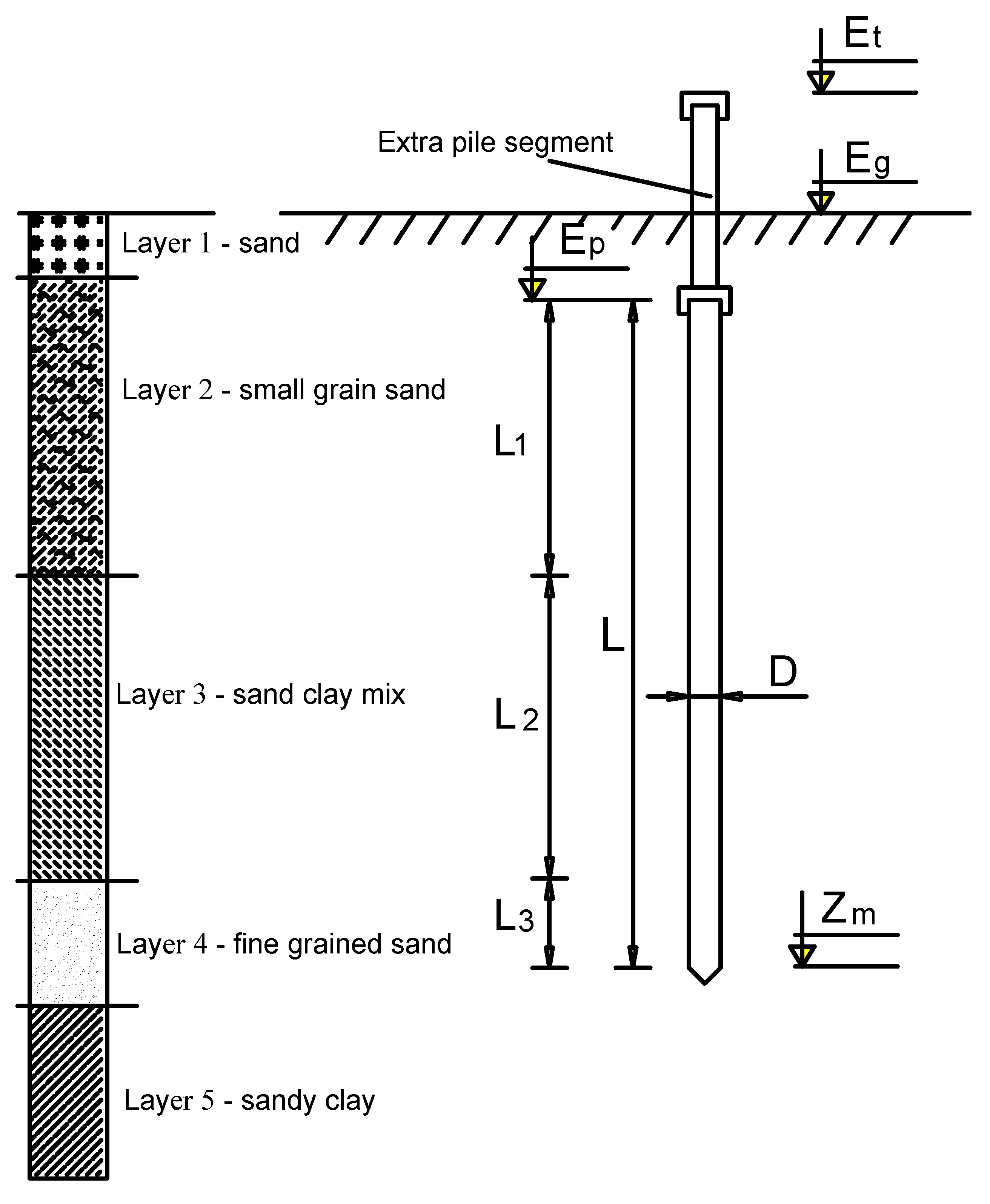
Hence, the factors that were used for ML simulation were (Figure 2): (i) pile diameter (D); (ii) length of pile tip segment (L1); (iii) length of second pile segment (L2); (iv) length of pile top segment (L3); (v) the natural ground elevation (Eg); (vi) pile top elevation (Ep); (vii) guide pile segment stop driving elevation (Et); (viii) pile tip elevation (Zm); (ix) the average SPT blow along the embedded length of the pile (Ns) and (x) the average SPT blow at the tip of the pile (Nt). The bearing capacity was the single output variable in this study (Pu).
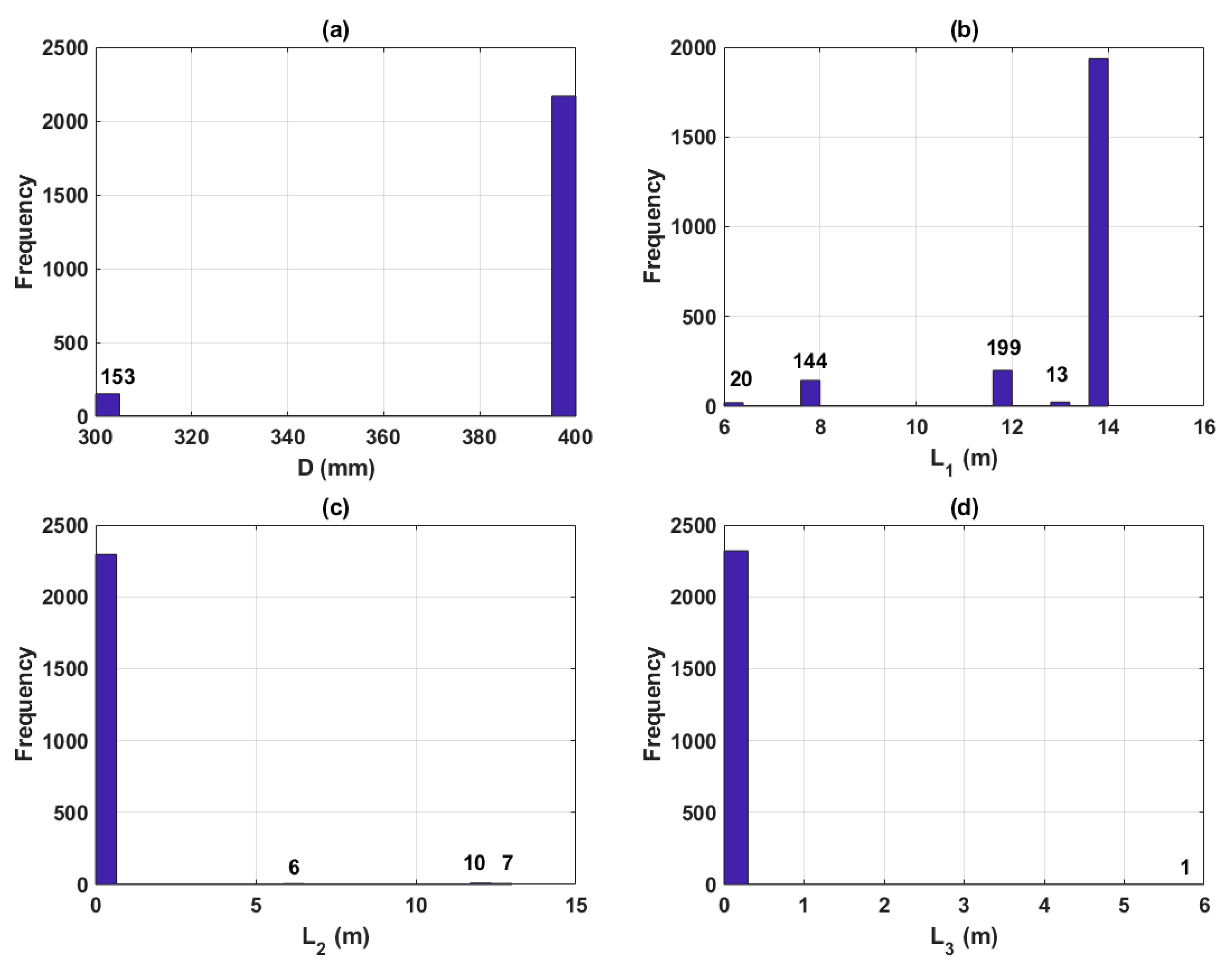
Due to an important quantity of data (2314 samples), the dataset used in this study is partly presented and summarized in Table 1, along with the statistical information of the input and output variables. As observed in Table 1, the pile diameter (D) ranged from 300 to 400 mm. The length of pile tip section (L1) ranged from 3 m to 8.4 m. The length of the second pile segment (L2) ranged from 1.47 m to 8 m. The length of pile top segment (L3) ranged from 0 m to 3.95 m, where a 0 value means that segment did not exist. The natural ground elevation (Eg) varied from −1.6 m to 3.4 m. The pile top elevation (Ep) varied from 2.05 m to 4.13 m. The guide piles stop driving elevation (Et) varied from −1.6 m to 8.4m. The pile tip elevation (Zm) varied from 8.27 m to 18.35 m. The average SPT blow counts along the embedded length of the pile (Ns) ranged from 5.57 to 19.2. The average SPT blow counts at the tip of the pile (Nt) ranged from 4.35 to 8.47. The bearing capacity load (Pu), ranged from 384 kN to 1860 kN with a mean value of 1164.5 kN and a standard deviation of 268.6 kN.
In this work, the collected dataset was divided into the training and testing datasets. The training part (approximately 70% of the total data) was used to train the ML models, whereas testing data (approximately 30% of the remaining dataset) was used to validate the performance of the ML models. Different from the original data, the training dataset (including 10 inputs and 1 output) was scaled in the [−1; 1] range (Table 2). By considering all variables in a uniform range, bias within the dataset between inputs could be minimized. In the present study, the range [−1; 1] was selected to better capture the non-Gaussian distribution of input variables. A scaling process of parameters, such as the minimum and maximum values of the training data were also used to scale the testing dataset. The scaling procedure of input and output variables was applied using Equation (1). Besides, the histograms of all the data, including 10 inputs and 1 output are presented in Figure 3.
where and represented the minimum and maximum values of the corresponding variables, and denoted the value of the selected input variable to be scaled.
4. Machine Learning Methods
4.1. Random Forest (RF)
Random Forests (RF) designate a family of ML methods, composed of different algorithms for inducing a set of decision trees, such as the Breiman Forest algorithm presented by Breiman [48] and often used in the literature as a benchmark model. In this algorithm, two principles of ‘randomization’ are used, namely the bagging and random feature selection. The learning step, therefore, consists in building a set of decision trees, each driven from a ‘bootstrap’ subset from the original learning set, i.e., using the bagging principle, and using a tree induction method called random tree. Such an induction algorithm, usually based on the classification and regression trees (CART) algorithm [49], modifies the partitioning procedure of the nodes of the tree so that the selection of the characteristic used as criterion of partitioning is partially random. In other words, for each node of the tree, a subset of characteristics is generated randomly, from which the best partitioning is achieved. To summarize, the RF method, a decision tree is constructed according to the following steps:
Step 1: For N data from the learning set, randomly draw N individuals with a discount. The resulting assembly will be the one used for the induction of the tree;
Step 2: For M characteristics, a number K << M is specified so that at each node of the tree, a subset of K characteristics is drawn randomly, among which the best is then selected for partitioning;
Step 3: The tree is constructed until it reaches its maximum size. No pruning is done. In this process, the induction of the tree is mainly directed by a hyperparameter, i.e., the number K. This number makes it possible to introduce more or less randomness into the induction.
In this way, except in the case of K = M, the induction of the tree is not at all ‘randomized’. Each tree in the forest has a structure and properties, which cannot be grasped. The randomness in RF induction could take advantage of the complementarity of trees, but there is no guarantee that adding a tree to the forest will actually improve the performance. Only a few research studies in the literature have looked at the number of decision trees to be built within a forest. When Breiman introduced the RF formalism in [48], the author also demonstrated that beyond a certain number of trees, adding others did not systematically improve the performance of RF. This result indicates that the number of trees in an RF does not necessarily have to be as large as possible to produce an efficient regressor. The results of [50,51] have experimentally confirmed this assertion.
4.2. Artificial Neural Network (ANN)
Artificial neural network (ANN) has emerged over the past four decades as a powerful and versatile computational tool for organizing and correlating knowledge [52]. ANN has been proved a useful prediction tool in solving many types of problems, usually difficult to address using conventional numerical and statistical approaches [53]. MeCulloch, the mathematician, and Pitts, the neuroscientist, are the first two scientists who developed the idea of ANN-based on the structure of the human brain [54]. The ANN has been proved to exhibit a strong ability to handle complex problems in which the relationships between input(s) and output(s) are complex or nonlinear [55]. This computational technique is capable of recognizing, capturing, and mapping features, the so-called ‘patterns’ in a set of data, primarily due to high neuronal interconnections that process much information in parallel [53]. The structure of ANN consists of several layers (input, hidden, and output layers) connected together by different link weights through hidden nodes [55]. In each node, the activation function is applied. The node net input is obtained by summing the weights of the connection as well as a bias [44]. The back-propagation is the most popular manner to train ANN among different learning algorithms [56]. In addition, many other rules of study have been introduced and extended to this day [57,58].
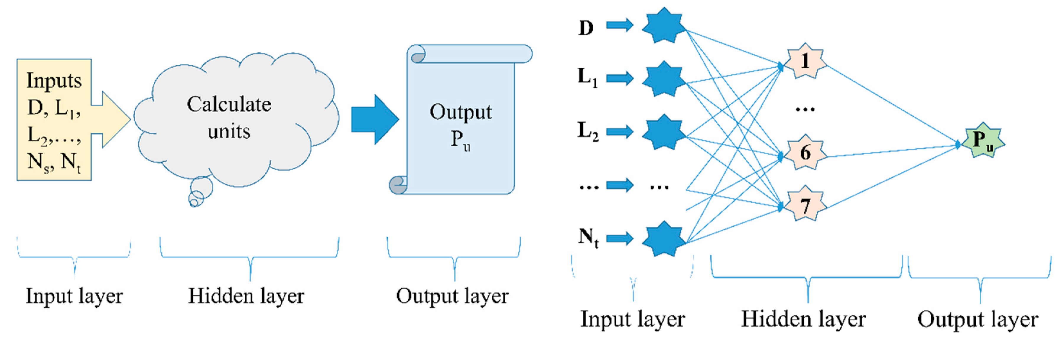
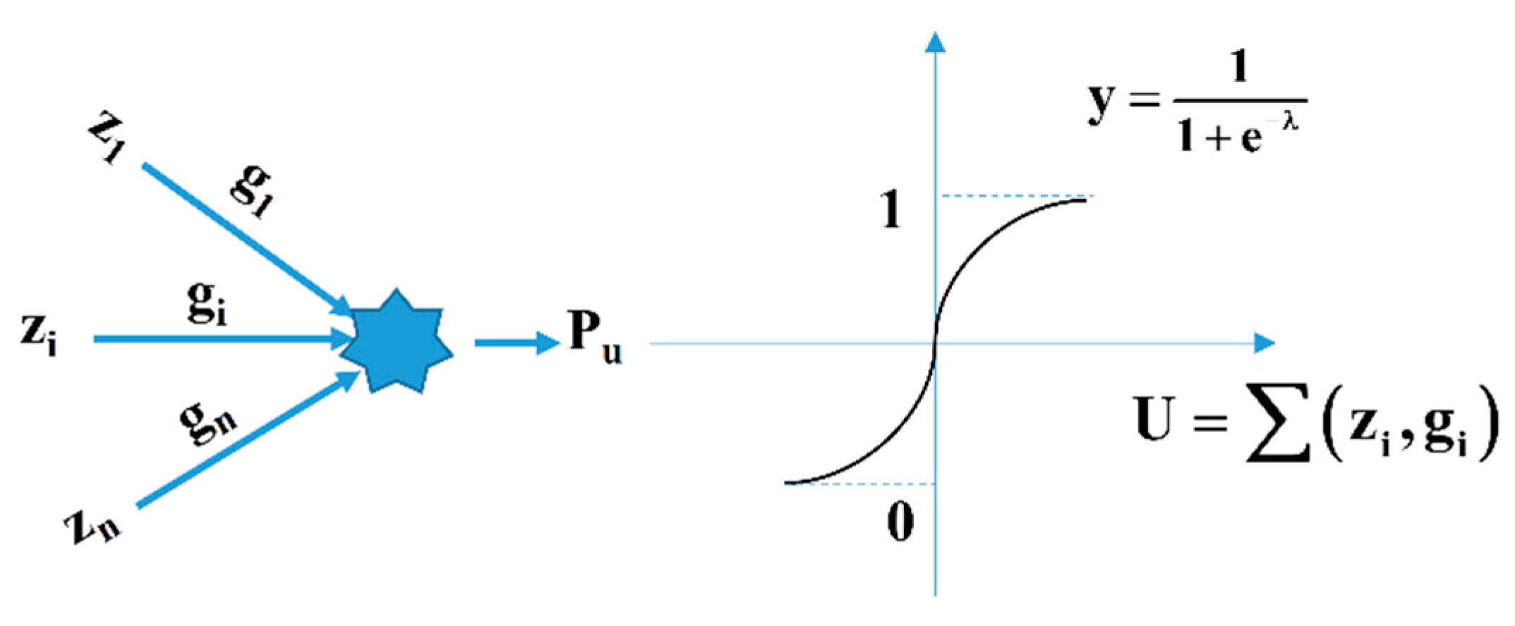
This fact shows that ANN has many advantages and is widely used in different fields, especially in the field of construction engineering [59,60]. Moreover, numerous investigations on the determination of bearing capacity using ANN have been conducted [53,55,57,58,60]. In the work of Pal and Deswal [61], the author predicted the total capacity of concrete spun pipe piles by using stress–wave data to build the ANN-based predictive model. Based on the conclusion, the predictive performance given by ANN was more reliable compared to supporting vector machines (SVM). Benaliand and Nechnech [62] proposed an ANN-based predictive model of cohesionless soil pile bearing efficiency. A number of 80 cases of axial load were used, and the results showed that the correlation coefficient (R) equaled to 0.92, showing the reliability of the ANN-based predictive model. Besides, numerous investigations on the behavior of pile bearing using ANN also pointed out a better prediction performance compared with analytical and empirical methods [53,60,61,62]. A schematic diagram of neural network could be illustrated in Figure 4. In the ANN algorithm, the multi-layer network is generally shown to operate most effectively, because it can simulate nonlinear processes. Neural computing’s main principle is the decomposition of the relationship between inputs and output into a series of linearly separable steps using hidden layers. Three distinct steps in developing an ANN-based solution could be summarized as [63]:
Step 1: Transformation or scaling of data;
Step 2: Definition of network architecture, where the number of hidden layers, the number of neurons in each layer, and the connectivity between neurons are determined. The network architecture selection could be depicted from Figure 4;
Step 3: Train the network to respond correctly a given set of inputs, this step is considered as the development of neural network (Figure 5);
4.3. Performance Evaluation
In this paper, three indicators accounting for the error between the actual and predicted values of Pu were used, namely the mean absolute error (MAE), root mean square error (RMSE), squared correlation coefficient, or the coefficient of determination (R2). The R2 measured the squared correlation between the predicted and actual Pu values, having values in the range of [0, 1]. Low RMSE and MAE values showed better accuracy of the proposed ML algorithms. On the other hand, RMSE calculated the squared root average difference, whereas MAE calculated the difference between the predicted and actual Pu values. These values could be calculated using the following equations [64,65,66,67,68]:
where inferred the number of the samples, and were the actual and predicted outputs, respectively, and was the average value of the .
5. Results and Discussion
5.1. Comparison of RF and ANN
The effectiveness of RF and ANN models is evaluated in this section. The parameters of ANN and RF used in this study are given in Table 3 and Table 4, respectively. The prediction performance in a regression form is shown in Figure 6 and Figure 7 for the training and testing datasets, respectively, whereas a summary of the corresponding information is indicated in Table 5. It is worth mentioning that the results presented herein were transformed into the normal range.
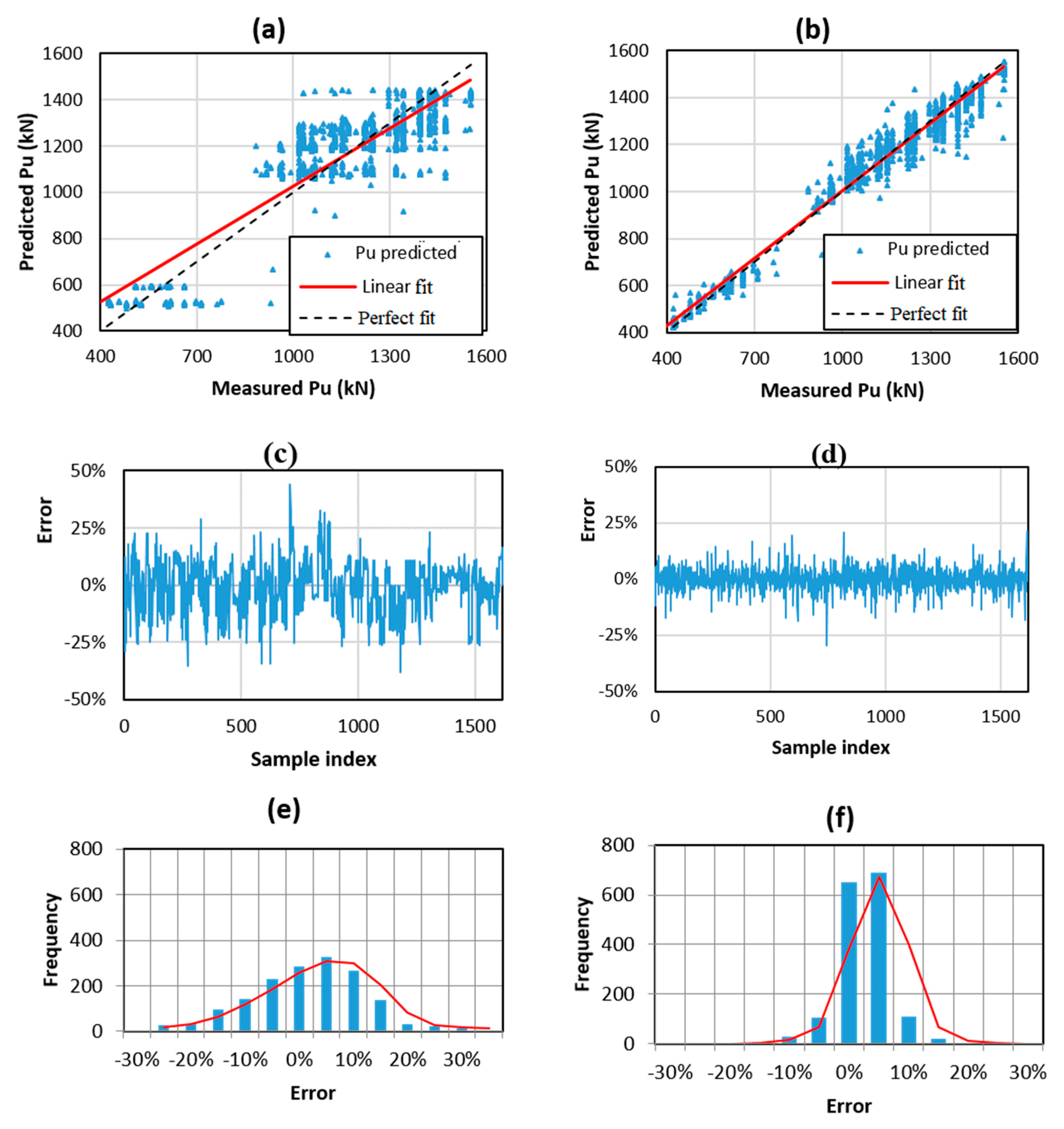
With respect to the training part, the RF model demonstrated a better performance, yielding a correlation of R2 = 0.969, RMSE = 47.333, and MAE = 2.178. The ANN model produced an intermediate accuracy (R2 = 0.818, RMSE = 114.882, and MAE = 1.050) for the training data. This was also confirmed by the values of the standard deviation of error (denoted as StDerror in Table 5). For the training part, RF yielded a lower value of StDerror compared to ANN (i.e., StDerror = 10.605% and 4.223% for ANN and RF, respectively).
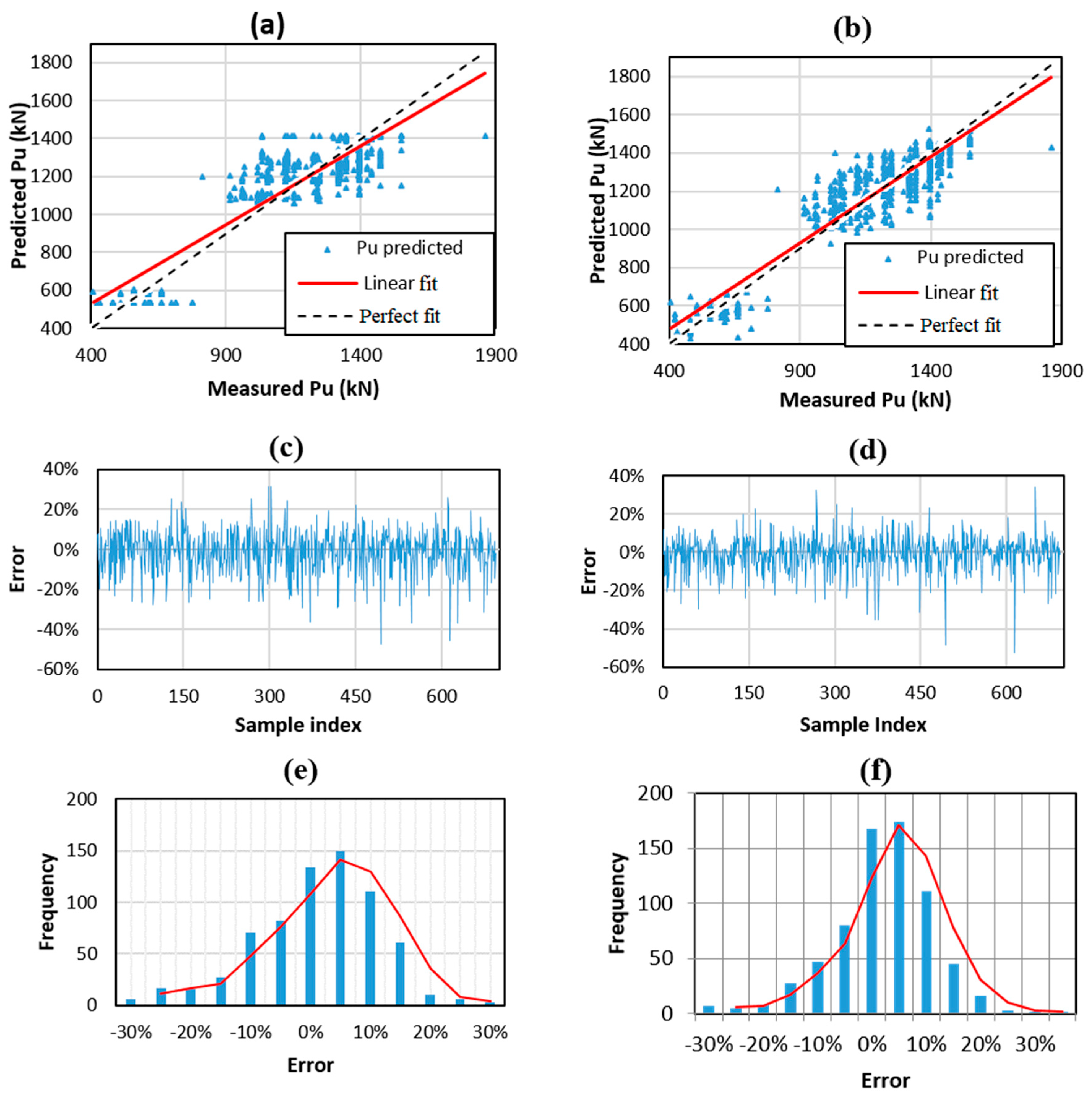
Considering the testing dataset, the RF model yielded the best prediction results with respect to R2, RMSE, MAE, the mean of error merror, and StDerror (i.e., R2 = 0.866, 0.809; RMSE = 98.161, 116.366; MAE = 2.924, 3.190; merror = 0.573%, 1.202%; StDerror =9.461%, 10.786% using RF and ANN, respectively). The MAE value of RF was slightly higher in the training part but much lower in the testing one compared to ANN because the performance of such a model might be influenced by choice of the selected index of the training data.
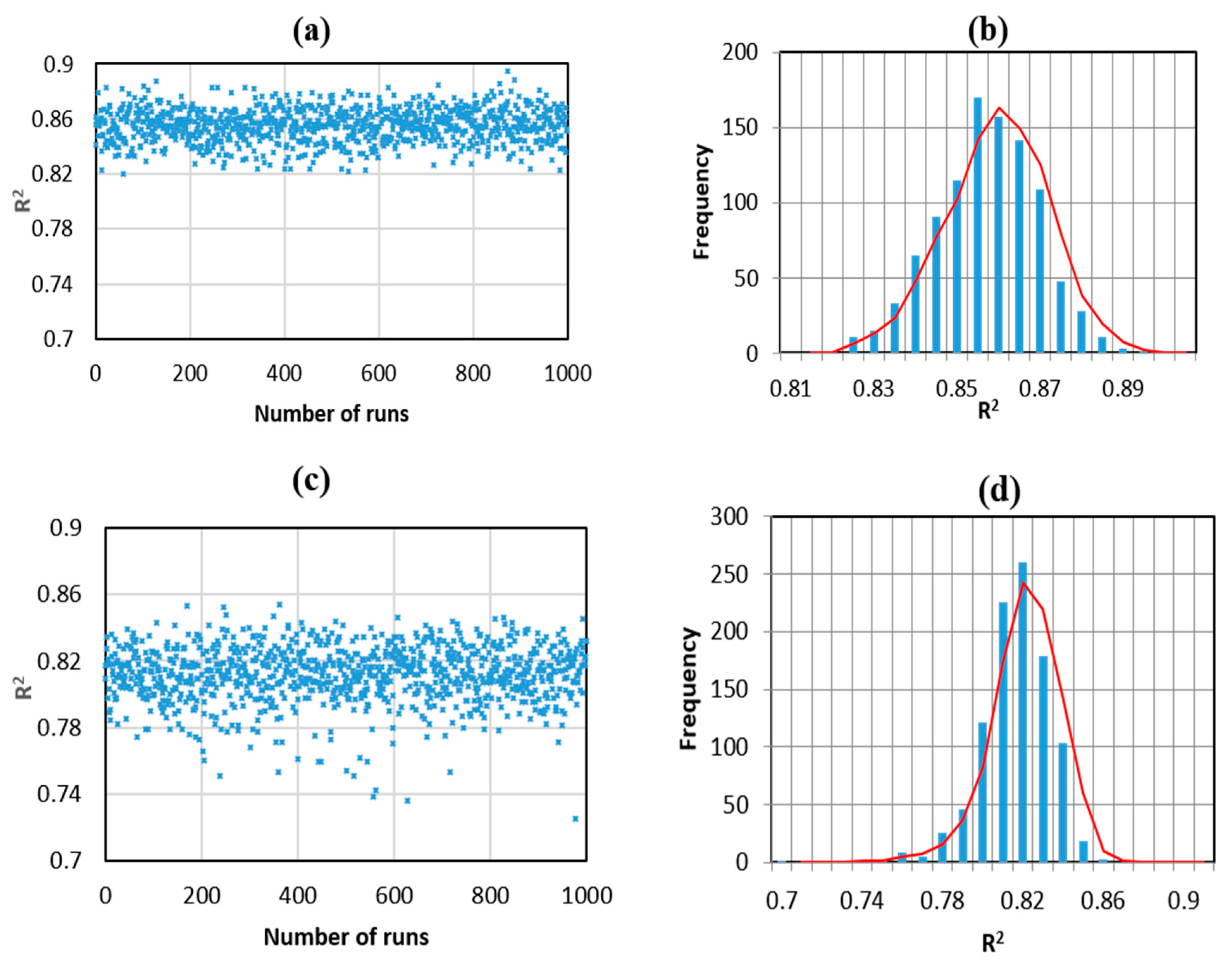
From a statistical point of view, the performance of ANN and RF algorithms needs to be fully evaluated. The above results showed that the RF model was better than ANN in predicting the bearing capacity of piles. As mentioned in the simulation procedure, 70% of the experimental data were randomly selected in order to construct and train the ANN and RF black boxes. The performance of such a model might be influenced by the choice of the sample indexes to construct the training dataset. Therefore, a total number of 1000 numerical simulations were next carried out, taking into account the random splitting effect in the dataset. The repetition of a simulation taking into account the random effect of input could also be called the Monte Carlo simulations, which is well-known in the literature [69]. The R2 values of these simulations are plotted in Figure 8a,c, and the corresponding histograms are plotted in Figure 8b,d. It was observed that the proposed RF model gave satisfactory R2 values within the range of 0.83 to 0.87. The most frequent R2 obtained over 1000 simulations was R2 = 0.855 with a frequency of about 170. Besides, ANN algorithm showed a lower accuracy when R2 values ranged from 0.78 to 0.84 with the most frequent values of R2 = 0.82 (frequency of about 260). Summarized values of the accuracy corresponded to the two models for the testing part is presented in Table 6.
It could thus be concluded that RF and ANN algorithms had high potential to predict the bearing capacity of driven piles. However, RF technique yielded better results with average R2 = 0.861 compare to ANN (average R2 = 0.811). In conclusion, from the statistical analysis and prediction errors, RF algorithm was the better model to predict the bearing capacity of pile.
5.2. Comparison with Empirical Equations and Multi-Variable Regression
In this section, comparisons of the RF model on the prediction of bearing capacity of driven piles are conducted with traditional formulas. These formulas used SPT value to estimate the bearing capacity of driven pile, as in the works of Meyerhof (1976) [4], Shioi and Fukui (1982) [7], Decourt (1995) [10], Shariatmadari et al. (2008) [8], and AIJ (2004) [11]. The values for unit base (Qb) and unit shaft (Qs) resistance are summarized in Table 7.
The value of the bearing capacity could be then estimated in function of Qb and Qs, following the well-known formula
where n refers to the number of soil layers, Li denotes the thickness and Qs(i) indicates the value for unit shaft resistance of the ith soil layer which piles penetrated through. In addition, the use of classical MVR to predict the bearing capacity of pile was also applied. Multi-variable regression technique is commonly used in several studies, such as Egbe et al. [70] and Silva et al. [71] to predict the properties and chemical composition of soil. The regression coefficient results are shown in Table 8.
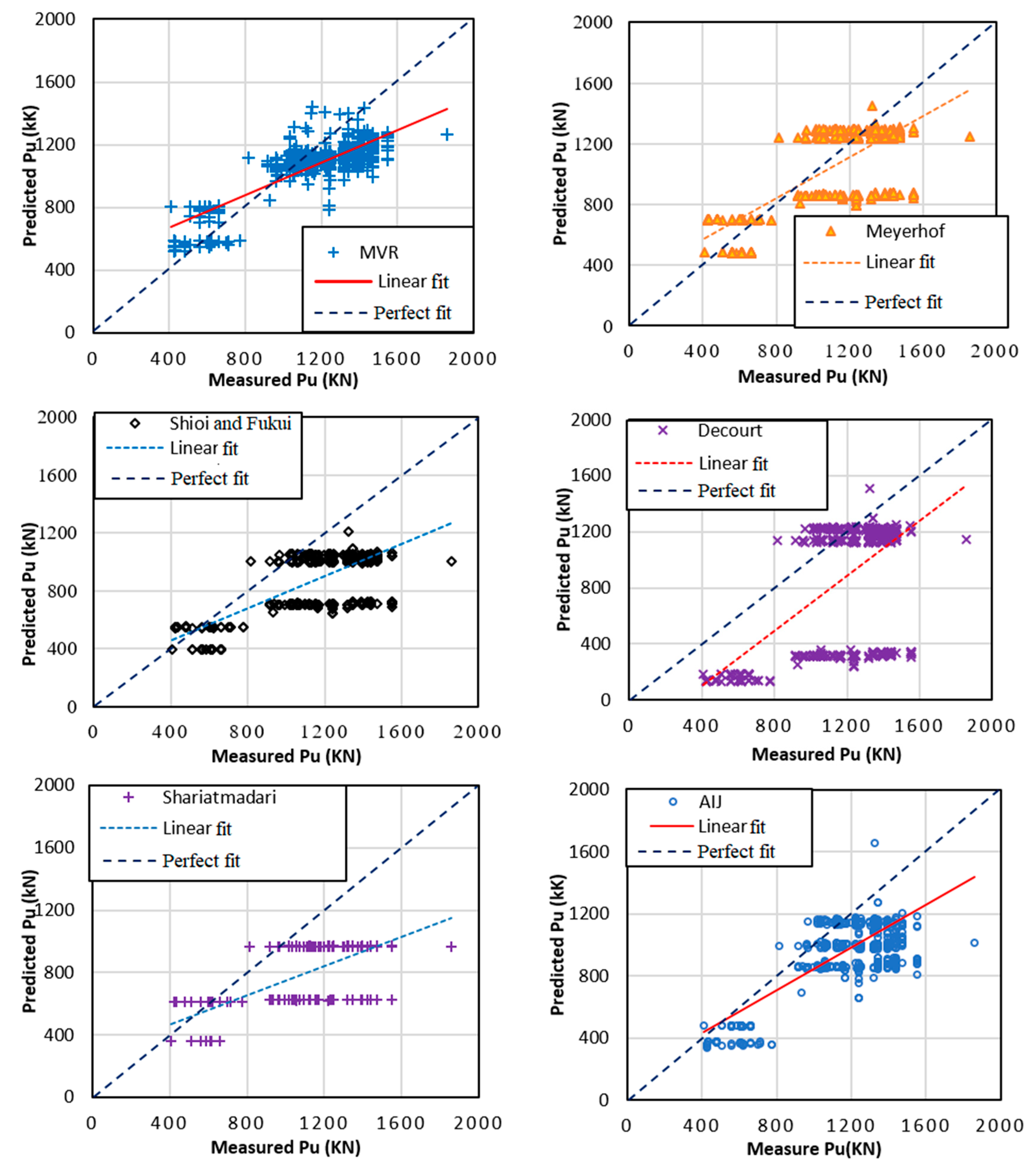
Figure 9 and Table 9 show several results and detail information of measured pile bearing capacity of the testing part, along with the bearing capacity predicted by RF model and MVR, Meyerhof (1976), Shioi and Fukui (1982), Decourt (1995), Shariatmadari (2008), and AIJ (2004). The RF was found the best model in predicting the experimental pile bearing capacity. Indeed, RF significantly outperformed traditional approaches with respect to R2, RMSE, MAE (i.e., R2 = 0.866, 0.702, 0.467, 0.485, 0.334, 0.391, 0.611; MAE = 2.924, 94.267, 77.830, 280.727, 312.297, 340.668, 205.72; RMSE = 98.161, 183.046, 224.5, 340.606, 483.335, 400.470, 265.53 using RF and Meyerhof (1976), Shioi and Fukui (1982), Decourt (1995), Shariatmadari (2008), and AIJ (2004), respectively). The results also showed that the MVR was less accurate than the RF model, but both models gave better accuracy than traditional formulas. It is worth noticing that these formulas were developed for granular soil. However, the effect of soil type in estimating the bearing capacity of piles was neglected in this study, knowing that such bearing capacity depends on soil types. The main purpose of this section was to demonstrate the higher prediction capacity of ML approach compared with empirical equations even without information related to soil types.
5.3. Feature Importance Analysis Using RF
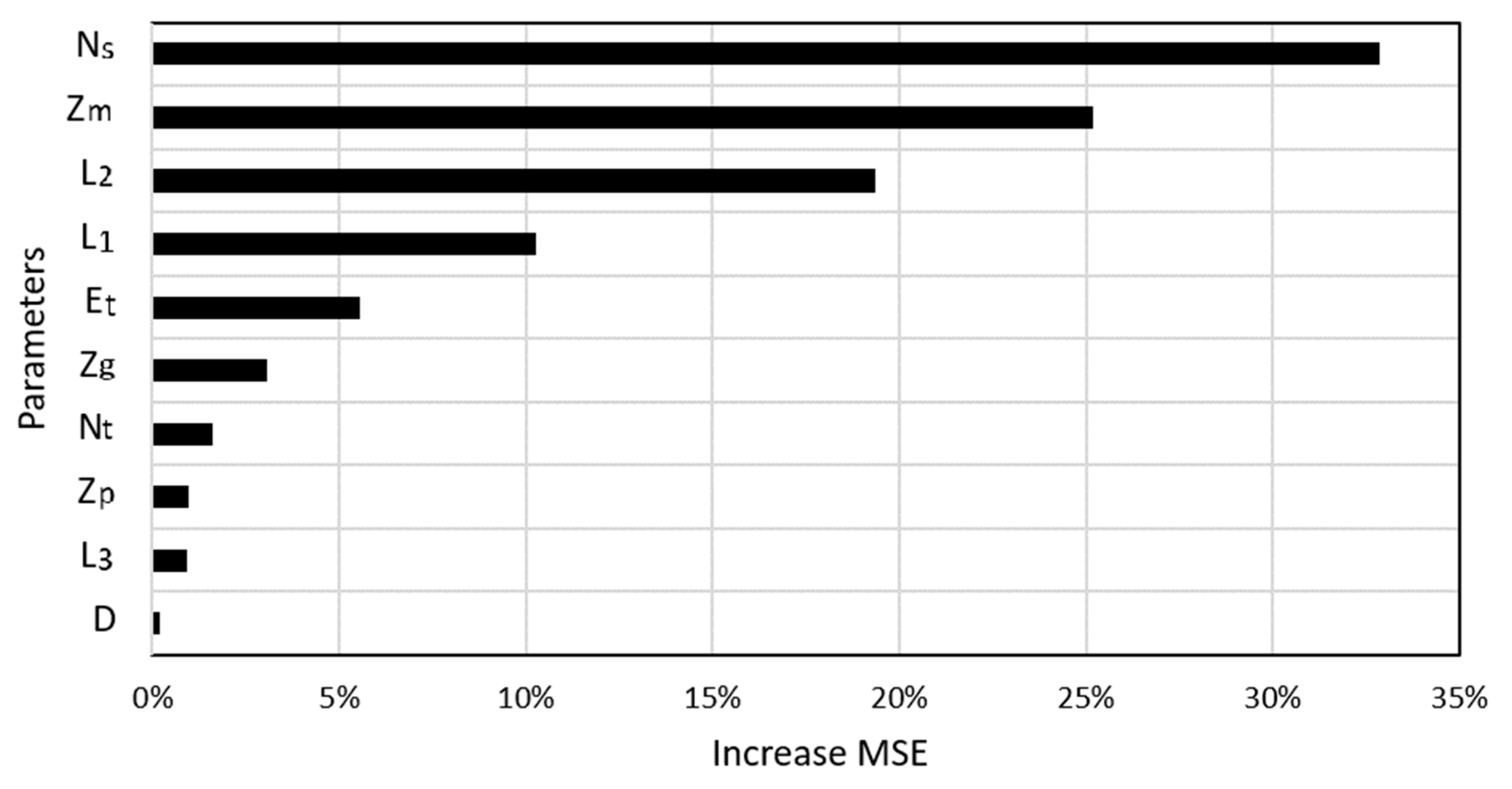
Basically, the RF algorithm allows evaluating the importance of input parameters. The importance of each predictor variable was measured as the change in the prediction accuracy (by an increase in mean square error—MSE), computed by permuting (value randomly shuffled) the variable with out-of-bag data in the random forests validation approach [72]. A more significant percentage of increase in mean square error indicates higher importance of a given variable in the prediction process [73]. The total sum percentage of the increase in the MSE of all variables is equal to 100%.
Amongst the 10 variables used to predict the bearing capacity of pile with RF, the average SPT blow along the embedded length of the pile (Ns) was the most important variable, as an increase in MSE of 33% was noticed (Figure 10). Indeed, Ns is an important indicator of predicting pile-bearing capacity, and it is related to the ultimate friction along the pile shaft. The pile tip elevation Zm was the second important variable, confirmed by an increase in MSE of 25%. From a soil mechanic point of view, it meant that with a little change in the soil properties, the pile tip elevation played an important role in the bearing capacity of pile; such a variable is involved in the pile tip resistance. The variables L2, L1, and Et were ranked as the third to the fifth important predictors, with an increase in MSE, ranging from 5% to 19% (Figure 10). Other predictor variables included in the model (Zg, Nt, Zp, L3, and D) had lower than 5% of the increase in MSE. This observation was also in good agreement with MVR results, where the coefficients of input variables L3 and Zp were equal to 0, while D had a relatively small coefficient of 2.33 (see Table 8).
6. Conclusions
In this study, the RF and ANN algorithms were used to examine the capability in predicting the bearing capacity of piles. An unprecedented database containing 2314 instances from on-field measurements of pile load test was used to develop and evaluate the two proposed ML models. The results showed that RF outperformed ANN with a satisfactory accuracy (R2 = 0.866, RMSE = 98.161 kN, MAE = 2.924 kN using RF compared with R2 = 0.809, RMSE = 116.366 kN, MAE =3.190 kN using ANN). Moreover, the results of this study indicated that the RF algorithm was more accurate in predicting the pile bearing capacity than those obtained from traditional approaches, namely the formulas or empirical equations from the work of Meyerhof (1976), Shioi and Fukui (1982), Decourt (1995), Shariatmadari (2008), AIJ (2004), and a classical MVR. In addition, a sensitivity analysis using RF indicated that the average SPT value along pile shaft Ns, pile tip elevation, and L2, L1, Et had the most significant effect on the predicted bearing capacity of piles.
Overall, the RF algorithm, like many other machine learning algorithms, has an additional advantage over conventional methods, which is, once the model is constructed, it can be used as an accurate, quick numerical tool for estimating the bearing capacity of piles. Thus, the performance of such a numerical tool is crucial in foundation engineering. Therefore, improving the prediction accuracy is one perspective of the present work, for instance, using hybrid ML algorithms or deep neural network to predict the bearing capacity of piles.
Author Contributions
Conceptualization, H.-B.L. and T.A.P.; Methodology, T.A.P., V.Q.T. and H.-L.T.V.; Software, T.A.P. and H.-B.L.; Validation, T.A.P.; Formal Analysis, T.A.P. and H.-B.L.; Investigation, T.A.P. and H.-B.L.; Resources, L.V.G., H.-A.T.D.; Data Curation, T.A.P. and L.V.G.; Writing-Original Draft Preparation, T.A.P., H.-B.L., V.Q.T. and H.-L.T.V.; Writing-Review & Editing, H.-B.L. and T.A.P.; Visualization, T.A.P. and H.-B.L.; Supervision, T.A.P., H.-B.L. and V.Q.T.; Project Administration, T.A.P. and H.-B.L.; Funding Acquisition, T.A.P. All authors have read and agreed to the published version of the manuscript.
Funding
This research received no external funding.
Conflicts of Interest
The authors declare no conflict of interest.
Appendix A
Figure A1.
Load–settlement relationship for pile number P_511.

Figure A2.
Load–settlement relationship for pile number P_140.

Figure A3.
Log–log load–settlement relationship for pile number P_140.

References
- Shooshpasha, I.; Hasanzadeh, A.; Taghavi, A. Prediction of the axial bearing capacity of piles by SPT-based and numerical design methods. Int. J. GEOMATE 2013, 4, 560–564. [Google Scholar] [CrossRef]
- Bond, A.J.; Schuppener, B.; Scarpelli, G.; Orr, T.L.L.; Dimova, S.; Nikolova, B.; Pinto, A.V.; European Commission; Joint Research Centre; Institute for the Protection and the Security of the Citizen. Eurocode 7: Geotechnical Design Worked Examples; Publications Office: Luxembourg, 2013; ISBN 978-92-79-33759-8. [Google Scholar]
- Bouafia, A.; Derbala, A. Assessment of SPT-based method of pile bearing capacity–analysis of a database. In Proceedings of the International Workshop on Foundation Design Codes and Soil Investigation in View of International Harmonization and Performance-Based Design, IWS Kamakura 2002, Tokyo, Japan, 10–12 April 2002; pp. 369–374. [Google Scholar]
- Meyerhof, G.G. Bearing Capacity and Settlement of Pile Foundations. J. Geotech. Eng. Div. 1976, 102, 197–228. [Google Scholar]
- Bazaraa, A.R.; Kurkur, M.M. N-values used to predict settlements of piles in Egypt. In Proceedings of In Situ ’86; New York, American Society of Civil Engineers: New York, NY, USA, 1986; pp. 462–474. [Google Scholar]
- Robert, Y. A few comments on pile design. Can. Geotech. J. 1997, 34, 560–567. [Google Scholar] [CrossRef]
- Shioi, Y.; Fukui, J. Application of N-value to design of foundations in Japan. In Proceedings of the Second European Symposium on Penetration Testing, ESOPT II, Amsterdam, The Netherlands, 24–27 May 1982; pp. 159–164. [Google Scholar]
- Shariatmadari, N.; Eslami, A.A.; Karim, P.F.M. Bearing capacity of driven piles in sands from SPT–applied to 60 case histories. Iran. J. Sci. Technol. Trans. B Eng. 2008, 32, 125–140. [Google Scholar]
- Lopes, R.F.; Laprovitera, H. On the prediction of the bearing capacity of bored piles from dynamic penetration tests. In Proceedings of the Deep Foundations on Bored and Auger Piles BAP III, Ghent, Belgium, 19–21 October 1998; A.A. Balkema: Rotterdam, The Netherlands; pp. 537–540. [Google Scholar]
- Decourt, L. Prediction of load-settlement relationships for foundations on the basis of the SPT. In Ciclo de Conferencias Internationale “Leonardo Zeevaert”; UNAM: Mexico City, Mexico, 1995; pp. 85–104. [Google Scholar]
- Architectural Institute of Japan. Recommendations for Design of Building Foundation; Architectural Institute of Japan: Tokyo, Japan, 2004. [Google Scholar]
- Asteris, P.G.; Ashrafian, A.; Rezaie-Balf, M. Prediction of the compressive strength of self-compacting concrete using surrogate models. Computers and Concrete. 2019, 24, 137–150. [Google Scholar]
- Asteris, P.G.; Moropoulou, A.; Skentou, A.D.; Apostolopoulou, M.; Mohebkhah, A.; Cavaleri, L.; Rodrigues, H.; Varum, H. Stochastic Vulnerability Assessment of Masonry Structures: Concepts, Modeling and Restoration Aspects. Appl. Sci. 2019, 9, 243. [Google Scholar] [CrossRef] [Green Version]
- Hajihassani, M.; Abdullah, S.S.; Asteris, P.G.; Armaghani, D.J. A gene expression programming model for predicting tunnel convergence. Appl. Sci. 2019, 9, 4650. [Google Scholar] [CrossRef] [Green Version]
- Huang, L.; Asteris, P.G.; Koopialipoor, M.; Armaghani, D.J.; Tahir, M.M. Invasive Weed Optimization Technique-Based ANN to the Prediction of Rock Tensile Strength. Appl. Sci. 2019, 9, 5372. [Google Scholar] [CrossRef] [Green Version]
- Le, L.M.; Ly, H.-B.; Pham, B.T.; Le, V.M.; Pham, T.A.; Nguyen, D.-H.; Tran, X.-T.; Le, T.-T. Hybrid Artificial Intelligence Approaches for Predicting Buckling Damage of Steel Columns Under Axial Compression. Materials 2019, 12, 1670. [Google Scholar] [CrossRef] [Green Version]
- Ly, H.-B.; Pham, B.T.; Dao, D.V.; Le, V.M.; Le, L.M.; Le, T.-T. Improvement of ANFIS Model for Prediction of Compressive Strength of Manufactured Sand Concrete. Appl. Sci. 2019, 9, 3841. [Google Scholar] [CrossRef] [Green Version]
- Ly, H.-B.; Le, L.M.; Duong, H.T.; Nguyen, T.C.; Pham, T.A.; Le, T.-T.; Le, V.M.; Nguyen-Ngoc, L.; Pham, B.T. Hybrid Artificial Intelligence Approaches for Predicting Critical Buckling Load of Structural Members under Compression Considering the Influence of Initial Geometric Imperfections. Appl. Sci. 2019, 9, 2258. [Google Scholar] [CrossRef] [Green Version]
- Ly, H.-B.; Le, T.-T.; Le, L.M.; Tran, V.Q.; Le, V.M.; Vu, H.-L.T.; Nguyen, Q.H.; Pham, B.T. Development of Hybrid Machine Learning Models for Predicting the Critical Buckling Load of I-Shaped Cellular Beams. Appl. Sci. 2019, 9, 5458. [Google Scholar] [CrossRef] [Green Version]
- Ly, H.-B.; Le, L.M.; Phi, L.V.; Phan, V.-H.; Tran, V.Q.; Pham, B.T.; Le, T.-T.; Derrible, S. Development of an AI Model to Measure Traffic Air Pollution from Multisensor and Weather Data. Sensors 2019, 19, 4941. [Google Scholar] [CrossRef] [PubMed] [Green Version]
- Xu, H.; Zhou, J.; Asteris, P.G.; Jahed Armaghani, D.; Tahir, M.M. Supervised Machine Learning Techniques to the Prediction of Tunnel Boring Machine Penetration Rate. Appl. Sci. 2019, 9, 3715. [Google Scholar] [CrossRef] [Green Version]
- Ly, H.-B.; Monteiro, E.; Le, T.-T.; Le, V.M.; Dal, M.; Regnier, G.; Pham, B.T. Prediction and Sensitivity Analysis of Bubble Dissolution Time in 3D Selective Laser Sintering Using Ensemble Decision Trees. Materials 2019, 12, 1544. [Google Scholar] [CrossRef] [Green Version]
- Chen, H.; Asteris, P.G.; Jahed Armaghani, D.; Gordan, B.; Pham, B.T. Assessing Dynamic Conditions of the Retaining Wall: Developing Two Hybrid Intelligent Models. Appl. Sci. 2019, 9, 1042. [Google Scholar] [CrossRef] [Green Version]
- Nguyen, H.-L.; Le, T.-H.; Pham, C.-T.; Le, T.-T.; Ho, L.S.; Le, V.M.; Pham, B.T.; Ly, H.-B. Development of Hybrid Artificial Intelligence Approaches and a Support Vector Machine Algorithm for Predicting the Marshall Parameters of Stone Matrix Asphalt. Appl. Sci. 2019, 9, 3172. [Google Scholar] [CrossRef] [Green Version]
- Nguyen, H.-L.; Pham, B.T.; Son, L.H.; Thang, N.T.; Ly, H.-B.; Le, T.-T.; Ho, L.S.; Le, T.-H.; Tien Bui, D. Adaptive Network Based Fuzzy Inference System with Meta-Heuristic Optimizations for International Roughness Index Prediction. Appl. Sci. 2019, 9, 4715. [Google Scholar] [CrossRef] [Green Version]
- Asteris, P.G.; Nozhati, S.; Nikoo, M.; Cavaleri, L.; Nikoo, M. Krill herd algorithm-based neural network in structural seismic reliability evaluation. Mech. Adv. Mater. Struct. 2019, 26, 1146–1153. [Google Scholar] [CrossRef]
- Asteris, P.G.; Armaghani, D.J.; Hatzigeorgiou, G.D.; Karayannis, C.G.; Pilakoutas, K. Predicting the shear strength of reinforced concrete beams using Artificial Neural Networks. Comput. Concr. 2019, 24, 469–488. [Google Scholar]
- Asteris, P.G.; Apostolopoulou, M.; Skentou, A.D.; Moropoulou, A. Application of artificial neural networks for the prediction of the compressive strength of cement-based mortars. Comput. Concr. 2019, 24, 329–345. [Google Scholar]
- Asteris, P.G.; Kolovos, K.G. Self-compacting concrete strength prediction using surrogate models. Neural Comput. Appl. 2019, 31, 409–424. [Google Scholar] [CrossRef]
- Asteris, P.G.; Mokos, V.G. Concrete compressive strength using artificial neural networks. Neural Comput. Appl. 2019. [Google Scholar] [CrossRef]
- Dao, D.V.; Ly, H.-B.; Trinh, S.H.; Le, T.-T.; Pham, B.T. Artificial Intelligence Approaches for Prediction of Compressive Strength of Geopolymer Concrete. Materials 2019, 12, 983. [Google Scholar] [CrossRef] [PubMed] [Green Version]
- Dao, D.V.; Trinh, S.H.; Ly, H.-B.; Pham, B.T. Prediction of Compressive Strength of Geopolymer Concrete Using Entirely Steel Slag Aggregates: Novel Hybrid Artificial Intelligence Approaches. Appl. Sci. 2019, 9, 1113. [Google Scholar] [CrossRef] [Green Version]
- Qi, C.; Ly, H.-B.; Chen, Q.; Le, T.-T.; Le, V.M.; Pham, B.T. Flocculation-dewatering prediction of fine mineral tailings using a hybrid machine learning approach. Chemosphere 2020, 244, 125450. [Google Scholar] [CrossRef] [PubMed]
- Pham, B.T.; Nguyen, M.D.; Dao, D.V.; Prakash, I.; Ly, H.-B.; Le, T.-T.; Ho, L.S.; Nguyen, K.T.; Ngo, T.Q.; Hoang, V.; et al. Development of artificial intelligence models for the prediction of Compression Coefficient of soil: An application of Monte Carlo sensitivity analysis. Sci. Total Environ. 2019, 679, 172–184. [Google Scholar] [CrossRef]
- Kumar, B.M.; Kumar, K.A.; Bharathi, A. Improved Soil Data Prediction Model Base Bioinspired K-Nearest Neighbor Techniques for Spatial Data Analysis in Coimbatore Region. Int. J. Future Revolut. Comput. Sci. Commun. Eng. 2017, 3, 345–349. [Google Scholar]
- Goh, A.T.C. Back-propagation neural networks for modeling complex systems. Artif. Intell. Eng. 1995, 9, 143–151. [Google Scholar] [CrossRef]
- Goh, A.T.C.; Kulhawy, F.H.; Chua, C.G. Bayesian Neural Network Analysis of Undrained Side Resistance of Drilled Shafts. J. Geotech. Geoenviron. Eng. 2005, 131, 84–93. [Google Scholar] [CrossRef]
- Shahin, M.A.; Jaksa, M.B. Neural network prediction of pullout capacity of marquee ground anchors. Comput. Geotech. 2005, 32, 153–163. [Google Scholar] [CrossRef]
- Shahin, M.A. Load–settlement modeling of axially loaded steel driven piles using CPT-based recurrent neural networks. Soils Found. 2014, 54, 515–522. [Google Scholar] [CrossRef] [Green Version]
- Shahin, M.A. State-of-the-art review of some artificial intelligence applications in pile foundations. Geosci. Front. 2016, 7, 33–44. [Google Scholar] [CrossRef] [Green Version]
- Shahin, M.A. Intelligent computing for modeling axial capacity of pile foundations. Can. Geotech. J. 2010, 47, 230–243. [Google Scholar] [CrossRef] [Green Version]
- Nawari, N.O.; Liang, R.; Nusairat, J. Artificial intelligence techniques for the design and analysis of deep foundations. Electr. J. Geotech. Eng. 1999, 4, 1–21. [Google Scholar]
- Pooya Nejad, F.; Jaksa, M.B.; Kakhi, M.; McCabe, B.A. Prediction of pile settlement using artificial neural networks based on standard penetration test data. Comput. Geotech. 2009, 36, 1125–1133. [Google Scholar] [CrossRef] [Green Version]
- Momeni, E.; Nazir, R.; Armaghani, D.J.; Maizir, H. Application of Artificial Neural Network for Predicting Shaft and Tip Resistances of Concrete Piles. Earth Sci. Res. J. 2015, 19, 85–93. [Google Scholar] [CrossRef]
- Bagińska, M.; Srokosz, P.E. The Optimal ANN Model for Predicting Bearing Capacity of Shallow Foundations trained on Scarce Data. KSCE J. Civ. Eng. 2019, 23, 130–137. [Google Scholar] [CrossRef] [Green Version]
- Teh, C.I.; Wong, K.S.; Goh, A.T.C.; Jaritngam, S. Prediction of Pile Capacity Using Neural Networks. J. Comput. Civil Eng. 1997, 11, 129–138. [Google Scholar] [CrossRef]
- De Beer, E.E. Proefondervindlijkebijdrage tot de studie van het grensdraagvermogen van zandonderfunderingen op staal; Tijdshift der OpenbarVerken van Belgie, No.6; NICI: Gent, Belgium, 1968. [Google Scholar]
- Breiman, L. Random Forests. Mach. Learn. 2001, 45, 5–32. [Google Scholar] [CrossRef] [Green Version]
- Breiman, L.; Friedman, J.; Stone, C.J.; Olshen, R.A. Classification and Regression Trees; Taylor & Francis: Oxfordshire, UK, 1984; ISBN 978-0-412-04841-8. [Google Scholar]
- Latinne, P.; Debeir, O.; Decaestecker, C. Limiting the Number of Trees in Random Forests. In Proceedings of the Second International Workshop on Multiple Classifier Systems, Cambridge, UK, 2–4 July 2001; pp. 178–187. [Google Scholar]
- Bernard, S.; Adam, S.; Heutte, L. Using Random Forests for Handwritten Digit Recognition. In Proceedings of the Ninth International Conference on Document Analysis and Recognition (ICDAR 2007), Curitiba, Parana, Brazil, 23–26 September 2007; pp. 1043–1047. [Google Scholar]
- Adeli, H. Neural Networks in Civil Engineering: 1989–2000. Comput. Aided Civil Infrastruct. Eng. 2001, 16, 126–142. [Google Scholar] [CrossRef]
- Tarawneh, B. Pipe pile setup: Database and prediction model using artificial neural network. Soils Found. 2013, 53, 607–615. [Google Scholar] [CrossRef] [Green Version]
- McCulloch, W.S.; Pitts, W. A logical calculus of the ideas immanent in nervous activity. Bull. Math. Biophys. 1943, 5, 115–133. [Google Scholar] [CrossRef]
- Momeni, E.; Nazir, R.; Armaghani, D.J.; Maizir, H. Prediction of pile bearing capacity using a hybrid genetic algorithm-based ANN. Measurement 2014, 57, 122–131. [Google Scholar] [CrossRef]
- Zaabab, A.H.; Zhang, Q.-J.; Nakhla, M. A neural network modeling approach to circuit optimization and statistical design. IEEE Trans. Microw. Theory Tech. 1995, 43, 1349–1358. [Google Scholar] [CrossRef]
- Das, S.K.; Basudhar, P.K. Undrained lateral load capacity of piles in clay using artificial neural network. Comput. Geotech. 2006, 33, 454–459. [Google Scholar] [CrossRef]
- Moayedi, H.; Armaghani, D.J. Optimizing an ANN model with ICA for estimating bearing capacity of driven pile in cohesionless soil. Eng. Comput. 2018, 34, 347–356. [Google Scholar] [CrossRef]
- Dao, D.V.; Adeli, H.; Ly, H.-B.; Le, L.M.; Le, V.M.; Le, T.-T.; Pham, B.T. A Sensitivity and Robustness Analysis of GPR and ANN for High-Performance Concrete Compressive Strength Prediction Using a Monte Carlo Simulation. Sustainability 2020, 12, 830. [Google Scholar] [CrossRef] [Green Version]
- Maizir, H.; Kassim, K.A. Neural network application in prediction of axial bearing capacity of driven piles. In Proceedings of the International Multiconference of Engineers and Computer Scientists, Hong Kong, China, 14–16 March 2013; Volume 2202, pp. 51–55. [Google Scholar]
- Pal, M.; Deswal, S. Modeling pile capacity using support vector machines and generalized regression neural network. J. Geotech. Geoenviron. Eng. 2008, 134, 1021–1024. [Google Scholar] [CrossRef]
- Benali, A.; Nechnech, A. Prediction of the pile capacity in purely coherent soils using the approach of the artificial neural networks. In Proceedings of the International Seminar, Innovation and Valorization in Civil Engineering and Construction Materials, Rabat, Morocco, 23–25 November 2011; pp. 23–25. [Google Scholar]
- Nehdi, M.; Djebbar, Y.; Khan, A. Neural network model for preformed-foam cellular concrete. Mater. J. 2001, 98, 402–409. [Google Scholar]
- Dao, D.V.; Jaafari, A.; Bayat, M.; Mafi-Gholami, D.; Qi, C.; Moayedi, H.; Phong, T.V.; Ly, H.-B.; Le, T.-T.; Trinh, P.T.; et al. A spatially explicit deep learning neural network model for the prediction of landslide susceptibility. CATENA 2020, 188, 104451. [Google Scholar] [CrossRef]
- Le, T.-T.; Pham, B.T.; Ly, H.-B.; Shirzadi, A.; Le, L.M. Development of 48-h Precipitation Forecasting Model using Nonlinear Autoregressive Neural Network. In CIGOS 2019, Innovation for Sustainable Infrastructure: Proceedings of the 5th International Conference on Geotechnics, Civil Engineering Works and Structures; Springer: Singapore, 2020; pp. 1191–1196. [Google Scholar]
- Pham, B.T.; Nguyen, M.D.; Ly, H.-B.; Pham, T.A.; Hoang, V.; Van Le, H.; Le, T.-T.; Nguyen, H.Q.; Bui, G.L. Development of Artificial Neural Networks for Prediction of Compression Coefficient of Soft Soil. In CIGOS 2019, Innovation for Sustainable Infrastructure: Proceedings of the 5th International Conference on Geotechnics, Civil Engineering Works and Structures; Springer: Singapore, 2020; pp. 1167–1172. [Google Scholar]
- Pham, B.T.; Le, L.M.; Le, T.-T.; Bui, K.-T.T.; Le, V.M.; Ly, H.-B.; Prakash, I. Development of advanced artificial intelligence models for daily rainfall prediction. Atmos. Res. 2020, 237, 104845. [Google Scholar] [CrossRef]
- Thanh, T.T.M.; Ly, H.-B.; Pham, B.T. A Possibility of AI Application on Mode-choice Prediction of Transport Users in Hanoi. In CIGOS 2019, Innovation for Sustainable Infrastructure: Proceedings of the 5th International Conference on Geotechnics, Civil Engineering Works and Structures; Springer: Singapore, 2020; pp. 1179–1184. [Google Scholar]
- Ly, H.-B.; Desceliers, C.; Le, L.M.; Le, T.-T.; Pham, B.T.; Nguyen-Ngoc, L.; Doan, V.T.; Le, M. Quantification of Uncertainties on the Critical Buckling Load of Columns under Axial Compression with Uncertain Random Materials. Materials 2019, 12, 1828. [Google Scholar] [CrossRef] [PubMed] [Green Version]
- Egbe, J.G.; Ewa, D.E.; Ubi, S.E.; Ikwa, G.B.; Tumenayo, O.O. Application of multilinear regression analysis in modeling of soil properties for geotechnical civil engineering works in Calabar South. Nig. J. Tech. 2018, 36, 1059. [Google Scholar] [CrossRef]
- Silva, S.H.G.; Teixeira, A.F.D.S.; Menezes, M.D.D.; Guilherme, L.R.G.; Moreira, F.M.D.S.; Curi, N. Multiple linear regression and random forest to predict and map soil properties using data from portable X-ray fluorescence spectrometer (pXRF). Ciênc. Agrotec. 2017, 41, 648–664. [Google Scholar] [CrossRef]
- Liaw, A.; Wiener, M. Classification and Regression by randomForest. R. News 2002, 2, 18–22. [Google Scholar]
- Zhang, B.; MacLean, D.; Johns, R.; Eveleigh, E. Effects of Hardwood Content on Balsam Fir Defoliation during the Building Phase of a Spruce Budworm Outbreak. Forests 2018, 9, 530. [Google Scholar] [CrossRef] [Green Version]
Figure 1.
(a) Experimental location; (b) pre-cast square-section concrete pile; (c) hydraulic pile presses machine; (d) experimental layout.
Figure 1.
(a) Experimental location; (b) pre-cast square-section concrete pile; (c) hydraulic pile presses machine; (d) experimental layout.

Figure 2.
Schematic diagram for soil stratigraphy and pile parameters.

Figure 3.
Histograms of the dataset in this study: (a) D; (b) L1; (c) L2; (d) L3; (e) Eg; (f) Ep; (g) Et; (h)Zm; (i) Ns; (j) Nt; (k) Pu.
Figure 3.
Histograms of the dataset in this study: (a) D; (b) L1; (c) L2; (d) L3; (e) Eg; (f) Ep; (g) Et; (h)Zm; (i) Ns; (j) Nt; (k) Pu.


Figure 4.
(Left) Schematic diagram of neural network and (Right) network architecture selection.

Figure 5.
Typical neural network development steps.

Figure 6.
Graphs of regression results between measured Pu versus predicted Pu for the training part using (a) ANN, (b) RF, (c) mean error ANN, (d) mean error RF, (e) standard deviation ANN, and (f) standard deviation RF.
Figure 6.
Graphs of regression results between measured Pu versus predicted Pu for the training part using (a) ANN, (b) RF, (c) mean error ANN, (d) mean error RF, (e) standard deviation ANN, and (f) standard deviation RF.

Figure 7.
Graphs of regression results between measured Pu versus predicted Pu for the testing part using (a) ANN, (b) RF, (c) mean error ANN, (d) mean error RF, (e) standard deviation ANN, and (f) standard deviation RF.
Figure 7.
Graphs of regression results between measured Pu versus predicted Pu for the testing part using (a) ANN, (b) RF, (c) mean error ANN, (d) mean error RF, (e) standard deviation ANN, and (f) standard deviation RF.

Figure 8.
Scatter plot of R2 values for 1.000 simulations for (a) RF, (c) ANN and the corresponding histograms of R2 values, (b) RF, (d) ANN.
Figure 8.
Scatter plot of R2 values for 1.000 simulations for (a) RF, (c) ANN and the corresponding histograms of R2 values, (b) RF, (d) ANN.

Figure 9.
Comparisons of pile bearing capacity prediction methods.

Figure 10.
Feature importance of 10 variables used in this study.


Table 1.
Inputs and output of the present study
| N° | D | L1 | L2 | L3 | Eg | Ep | Et | Zm | Ns | Nt | Pu |
|---|---|---|---|---|---|---|---|---|---|---|---|
| Unit | mm | m | m | m | m | m | m | m | - | - | kN |
| 1 | 400 | 3.45 | 8 | 0.07 | 2.95 | 3.42 | 2.95 | 14.47 | 11.52 | 7.44 | 1163 |
| 2 | 400 | 3.4 | 7.29 | 0 | 3.4 | 3.49 | 3.4 | 14.09 | 10.69 | 7.27 | 1240 |
| 3 | 400 | 4.35 | 8 | 1.2 | 2.05 | 3.4 | 5.8 | 15.6 | 13.55 | 7.74 | 1297.8 |
| . | . | . | . | . | . | . | . | . | . | . | . |
| . | . | . | . | . | . | . | . | . | . | . | . |
| . | . | . | . | . | . | . | . | . | . | . | . |
| 2312 | 400 | 5.72 | 8 | 1.67 | 0.68 | 4.13 | 1.06 | 16.07 | 15.39 | 7.50 | 1344 |
| 2313 | 400 | 4.1 | 2.19 | 0 | 2.7 | 3.72 | 2.73 | 8.99 | 6.29 | 4.94 | 480 |
| 2314 | 400 | 4.05 | 8 | 0.7 | 2.35 | 3.5 | 2.4 | 15.1 | 12.75 | 7.58 | 1318 |
| Min | 300 | 3.00 | 1.47 | 0.00 | −1.60 | 2.05 | −1.60 | 8.27 | 5.57 | 4.35 | 384 |
| Average | 393.3 | 4.02 | 7.27 | 0.49 | 2.53 | 3.52 | 2.70 | 14.30 | 11.78 | 7.24 | 1164.5 |
| Max | 400 | 8.40 | 8.00 | 3.95 | 3.40 | 4.13 | 8.40 | 18.35 | 19.20 | 8.47 | 1860 |
| SD | 24.85 | 0.55 | 1.53 | 0.50 | 0.63 | 0.09 | 0.75 | 1.68 | 2.02 | 0.71 | 268.63 |
SD = Standard deviation.
Table 2.
Statistical values of the normalization process of the training dataset
| D | L1 | L2 | L3 | Eg | Ep | Et | Zm | Ns | Nt | |
|---|---|---|---|---|---|---|---|---|---|---|
| Min | −1.0 | −1.0 | −1.0 | −1.0 | −1.0 | −1.0 | −1.0 | −1.0 | −1.0 | −1.0 |
| Average | 0.868 | 0.845 | −0.983 | −0.999 | 0.651 | 0.410 | −0.139 | 0.197 | 0.401 | 0.284 |
| Max | 1.0 | 1.0 | 1.0 | 1.0 | 1.0 | 1.0 | 1.0 | 1.0 | 1.0 | 1.0 |
| SD | 0.497 | 0.413 | 0.172 | 0.042 | 0.253 | 0.084 | 0.150 | 0.333 | 0.342 | 0.959 |
SD = Standard deviation.
Table 3.
ANN parameters used in this study
| Parameters | Value and Description |
|---|---|
| Number of neurons in the input layer | 10 |
| Number of hidden layers | 1 |
| Number of neurons in the hidden layer | 7 |
| Number of neurons in the output layer | 1 |
| Activation function for the hidden layer | Logistic |
| Activation function for the output layer | Linear |
| Training algorithm | Quasi-Newton methods |
| Cost function | Mean Square Error (MSE) |
Table 4.
RF parameters used in this study
| Parameters | Value and Description |
|---|---|
| Number of trees | 15 |
| Number of features to consider when looking for the best split | 10 |
| Minimum number of samples required to split an internal node | 2 |
| Minimum number of samples required to be at a leaf node | 1e-7 |
| Cost function | Mean Square Error (MSE) |
| Maximum depth of the tree | None |
Table 5.
Summary of prediction capability
| Part | Method | R2 | MAE (kN) | RMSE (kN) | merror (%) | StDerror (%) |
|---|---|---|---|---|---|---|
| Training | ANN | 0.818 | 1.050 | 114.882 | 0.884% | 10.605% |
| RF | 0.969 | 2.178 | 47.333 | 0.069% | 4.223% | |
| Testing | ANN | 0.809 | 3.190 | 116.366 | 1.202% | 10.786% |
| RF | 0.866 | 2.924 | 98.161 | 0.573% | 9.461% |
Table 6.
Summary of the Monte Carlo simulations
| Part | Method | Avr. R2 | StD. R2 |
|---|---|---|---|
| Testing | ANN | 0.811 | 0.318 |
| RF | 0.861 | 0.277 |
Table 7.
Comparison of SPT methods for predicting the pile bearing capacity
| Ground Type | Sandy Ground | Clayey Ground |
|---|---|---|
| Meyerhof (1976) [4] | ||
| Shioi and Fukui (1982) [7] | ||
| Decourt (1995) [10] | ||
| Shariatmadari (2008) [8] | ||
| AIJ (2004) [11] | ||
Table 8.
MVR coefficients
| Variable | Intercept | D | L1 | L2 | L3 | Zp | Zg | Et | Zm | Ns | Nt |
|---|---|---|---|---|---|---|---|---|---|---|---|
| Coefficients | −611.39 | 2.33 | 86.29 | 142.11 | 0 | 0 | −54.05 | 62.09 | 31.85 | 23.16 | −169.43 |
Table 9.
Summary of different pile bearing capacity prediction methods
| RF Model | MVR | Meyerhof (1976) | Shioi and Fukui (1982) | Decourt (1995) | Shariatmadari (2008) | AIJ (2004) | |
|---|---|---|---|---|---|---|---|
| R2 | 0.866 | 0.702 | 0.467 | 0.485 | 0.334 | 0.391 | 0.611 |
| MAE (kN) | 2.924 | 94.267 | 77.830 | 280.727 | 312.297 | 340.668 | 205.721 |
| RMSE(kN) | 98.161 | 183.046 | 224.500 | 340.606 | 483.335 | 400.470 | 265.531 |
© 2020 by the authors. Licensee MDPI, Basel, Switzerland. This article is an open access article distributed under the terms and conditions of the Creative Commons Attribution (CC BY) license (http://creativecommons.org/licenses/by/4.0/).
Share and Cite
MDPI and ACS Style
Pham, T.A.; Ly, H.-B.; Tran, V.Q.; Giap, L.V.; Vu, H.-L.T.; Duong, H.-A.T. Prediction of Pile Axial Bearing Capacity Using Artificial Neural Network and Random Forest. Appl. Sci. 2020, 10, 1871. https://doi.org/10.3390/app10051871
AMA Style
Pham TA, Ly H-B, Tran VQ, Giap LV, Vu H-LT, Duong H-AT. Prediction of Pile Axial Bearing Capacity Using Artificial Neural Network and Random Forest. Applied Sciences. 2020; 10(5):1871. https://doi.org/10.3390/app10051871
Chicago/Turabian StylePham, Tuan Anh, Hai-Bang Ly, Van Quan Tran, Loi Van Giap, Huong-Lan Thi Vu, and Hong-Anh Thi Duong. 2020. "Prediction of Pile Axial Bearing Capacity Using Artificial Neural Network and Random Forest" Applied Sciences 10, no. 5: 1871. https://doi.org/10.3390/app10051871
Note that from the first issue of 2016, this journal uses article numbers instead of page numbers. See further details here.