An Optimized Covering Spheroids by Spheres
by
 and
and
Alexander Pankratov
1, 
Tatiana Romanova
1,
Igor Litvinchev
2 and
Jose Antonio Marmolejo-Saucedo
3,* 1
Department of Mathematical Modeling and Optimal Design, Institute for Mechanical Engineering Problems of the National Academy of Sciences of Ukraine Kharkov 61046, Ukraine, Kharkiv National University of Radioelectronics, Kharkov 61166, Ukraine
2
Faculty of Mechanical and Electrical Engineering, Graduate Program in Systems Engineering, Nuevo Leon State University (UANL), Monterrey 66450, Mexico
3
Facultad de Ingeniería, Universidad Panamericana, Augusto Rodin 498, Ciudad de Mexico 03920, Mexico
*
Author to whom correspondence should be addressed.
Appl. Sci. 2020, 10(5), 1846; https://doi.org/10.3390/app10051846
Submission received: 29 December 2019
/
Revised: 3 March 2020
/
Accepted: 3 March 2020
/
Published: 7 March 2020
(This article belongs to the Special Issue Applied Optimization in Clean and Renewable Energy: New Trends)
Abstract
:Covering spheroids (ellipsoids of revolution) by different spheres is studied. The research is motivated by packing non-spherical particles arising in natural sciences, e.g., in powder technologies. The concept of an -cover is introduced as an outer multi-spherical approximation of the spheroid with the proximity . A fast heuristic algorithm is proposed to construct an optimized -cover giving a reasonable balance between the value of the proximity parameter and the number of spheres used. Computational results are provided to demonstrate the efficiency of the approach.
1. Introduction
Covering a certain region by simple shapes has various applications. Our interest in covering problems is motivated by packing particles arising in science and engineering applications. Packing problems are widely used in modeling liquid and glass structures [1,2], representing granular materials [3], packing beds, and cermet [4], as well as in many other applications (see, e.g., [5,6,7,8,9,10]). Many algorithms have been proposed for packing spherical particles (see, e.g., [11,12,13,14,15,16] and the references therein). However, to have a better and more adequate representation of particulate microstructure, packing non-spherical particles must be considered. The approaches proposed to handle non-spherical shapes can be divided in three large groups [17]. Techniques in the first group use analytical equations for the shapes of the particles, e.g., ellipsoids, and the main modeling problem is to state analytically non-overlapping and containment conditions [18,19,20,21,22,23]. The second approach is based on tessellating the container/particles shapes with a grid and then approximating them by corresponding collections of grid nodes (see, e.g., [15,24] and the references therein). This way, detecting the overlap is reduced to verify if two shapes share the same node. However, to get a reasonable approximation, fine grids must be used resulting in large-scale and memory-consuming problems. In the third approach, the shape of the particle is represented approximately by a collection of spheres having different sizes and positions (see, e.g., [25,26,27]). Then, detecting the overlap is reduced to verifying the overlapping for two spheres from different particle collections. This problem is much simpler than detecting overlapping in the first approach. The third approach can be considered as a compromise between the simplicity of the tessellating techniques and the rigor of the methods based on analytical shapes presentation. The efficiency of the third approach depends on the quality of the multi-spherical approximation of the shape of the particle. The number of the spheres representing the shape of the particle must be small enough to simplify the non-overlapping (pairwise) test. At the same time, the union of the spheres in the collection must represent the original shape of the particle closely enough.
Among the different shapes used to represent the microstructure of non-spherical particles, the spheroid (ellipsoid of revolution) is one of the most frequently used (see, e.g., [5,6,7,8,10]). One of the reasons to use the spheroid is its relative simplicity comparing to the general ellipsoid. Moreover, in many cases, analyses of 3D spheroids are reduced to the examination of the 2D ellipses used to generate the spheroid.
In this paper, the problem of covering the spheroid by different spheres is studied. An -cover is introduced as an outer multi-spherical approximation of the spheroid within the error . A fast heuristic algorithm is proposed to construct the optimized -cover giving a reasonable balance between the value of the proximity parameter and the number of spheres used. Computational results are provided to demonstrate efficiency of the approach.
The main contributions of the paper are as follows:
- The concept of the -cover is introduced for the outer multi-spherical approximation of the spheroid.
- A fast two-stage approach is proposed to get a reasonable (optimized) -cover.
- Numerical results are provided to illustrate the main constructions.
The paper is organized as follows. Section 2 presents the basic definitions and formulations used in the paper as well as the two-stage conceptual approach. Solution techniques are presented in detail in Section 3. Numerical results are presented in Section 4, while Section 5 presents the conclusions. Expressions for the parameters used in Section 3 are derived in the Appendix A.
2. Basic Constructions
The following definitions are used throughout the paper. Let
be a given spheroid (ellipsoid of revolution) with .
Definition 1.
A setis called a cover (outer approximation) for the spheroid if .
The following extended spheroid, referred to as an -spheroid,
can be considered as an outer approximation of the original spheroid with a given error .
Definition 2.
setis called an-cover if, whereis an error of the cover.
In this paper, the -cover of the spheroid by spheres , is studied. The multi-spherical -cover is denoted by , i.e., .
From a practical point of view, a “good” -cover must use a few circles and provide a small approximation error . However, we may expect that for sufficiently small , decreasing in results in increasing , and vice versa. Thus, we cannot minimize and simultaneously. Instead, our problem is formulated as follows:
Find , i.e., positions, radii and total number of spheres, providing a reasonable balance between and .
The following heuristic two-stage approach is proposed to construct the optimized -cover.
Stage 1. For a given , find the minimum number of the spheres covering the given spheroid ; i.e., find . Here, the decision variables are the positions and radii of the circles and their total number .
Stage 2. For obtained at Stage 1, find a cover of the given spheroid with the minimal value ; i.e., find . Here, the decision variables are the positions and radii of the circles and the proximity parameter .
In what follows, constructing the cover is referred to as an Optimized Spherical Covering (OSC). Detailed descriptions of problems arising at Stages 1,2 and their solutions are presented in the next section.
3. Solution Algorithm
Let an ellipse with semi-axes and be the projection of the spheroid on the plane XOY. It is assumed that the centers of the spheres of variable radii belong to the axis OX, i.e., .
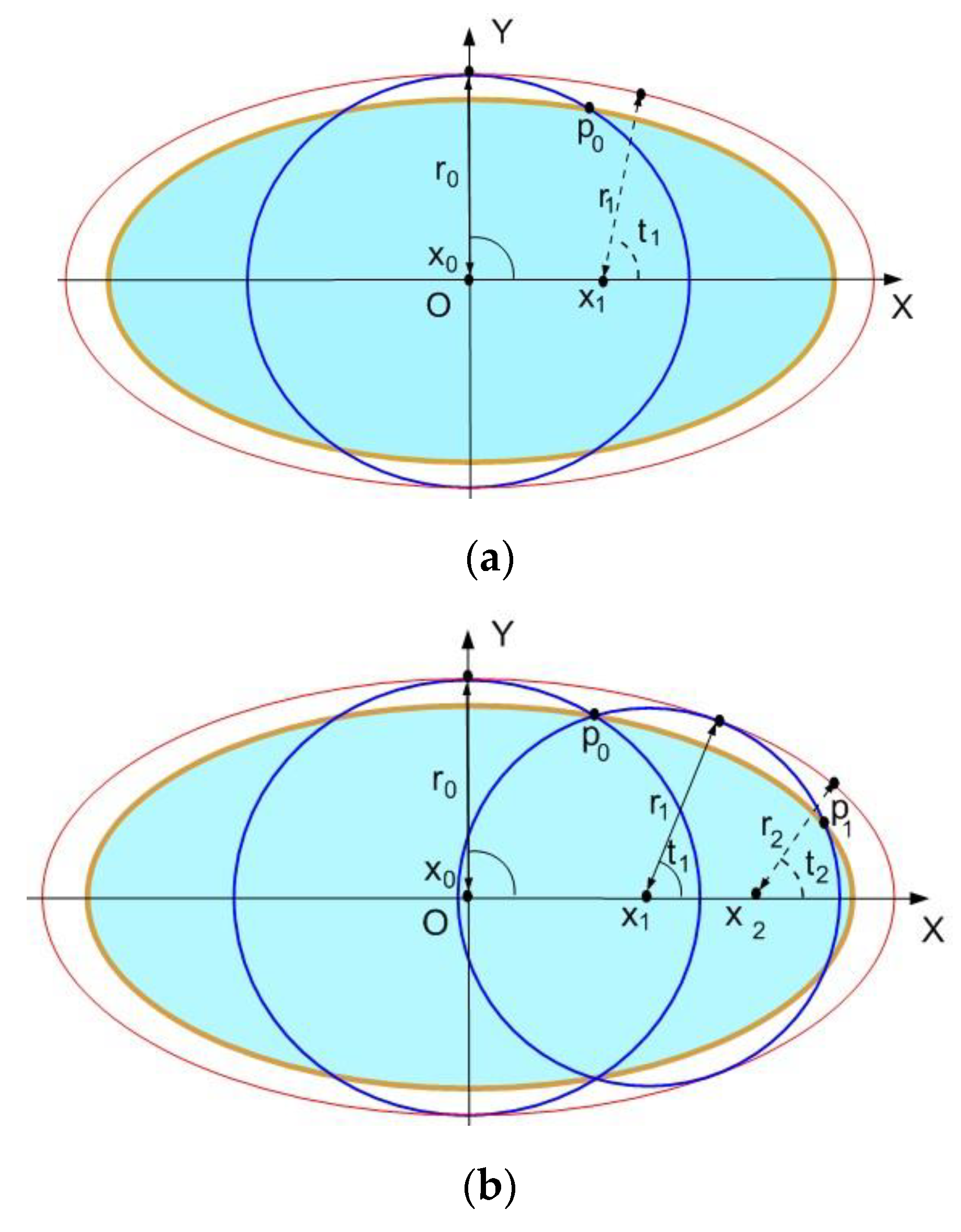
Note that the point belongs to the axis OX for . Denote by the cover that is the projection of on the plane XOY. By the definition, the cover is an outer approximation of the ellipse , i.e., Suppose that the odd number of the circles is used for the cover, and the first circle has its radius and is centered at the point , as shown at Figure 1a. Then, due to the symmetry, the ellipse can be covered by a collection of circles. Here, the right-hand side of the can be covered by the circles with , , and similarly the left-hand side.
For the case of an even number of circles, the ellipse be covered by a collection of circles . Let the first circle be centered at the point , as shown at Figure 1b. To find the parameters of the first circle for , the following optimization problem is solved:
For the given corresponding parameters are defined in the form of
Using the parametric description of the ellipse [28], the parameter can be obtained analytically as follows (we would like to thank the anonymous referee for pointing out the possibility of getting the explicit solution):
The details are presented in the Appendix A.
Then, due to the symmetry, the right-hand side of the ellipse can be covered by a collection of circles , for , and similarly for the left-hand side.
In what follows, the solution algorithm for the OSC problem is presented only for the odd number of spheres, since the difference between the odd and even cases is only in the parameters of the first sphere.
3.1. Solution Algorithm for Stage 1
Let the value of be given.
At Stage 1, the objective is to find the minimum number of circles covering the ellipse centered at for the given value of .
Step 1. Set , , , , , where , are the sizes of the ellipse .
Step 2. Get the intersection point of the ellipse E and the circle solving the following system:
where is the radius of the circle centered at the point .
Using the parametric description of the ellipse [28], the point is presented analytically by the following formula (see the Appendix A for details):
Step 3. Set .
Step 4. Solve the following nonlinear programming problem:
and get its optimal solution . Here, the feasible set is defined by the following system of inequalities:
where inequality (5) assures that the point is inside the circle of radius centered at ; inequality (6) guarantees that the circle of radius centered at is inside the ellipse with semi-axes , ; inequality (7) reflects the monotonous decrease of the corresponding angle ; and the last inequality describes the natural constraint for the radius of the circle . Find Using the parametric description of the ellipse [28], the parameters and are presented analytically in the following form (see the Appendix A for details):
Step 5. If the point is inside the circle of radius centered at , then the solution is obtained and the algorithm stops. Otherwise, go to Step 2.
3.2. Solution Algorithm for the Stage 2
At this stage, the minimum value of is obtained for a given number of covering circles.
Let be the ellipse centered at with semi-axes , (see Figure 4).
The points , , , which are referred to as the pilot points, are introduced for the “gluing” circles , .
Let , , , , , and . Here, is the parameter (angle) introduced in Equations (3)–(4) and obtained at Stage 1.
The following nonlinear programing problem is used to optimize :
Here, is the -dimensional vector of unknown variables and the feasible set is defined by the following system of inequalities:
Here, inequality (9) assures ; inequality (10) reflects the monotonous decrease of the corresponding angle ; inequality (11) describes the natural constraint for the radius of the circle ; constraints (12) guarantee ; inequalities (13) present the nonnegativity of all ; constraints (14) and (15) assure , while (16) guarantees .
4. Computational Results
Computational experiments were run on an AMD Athlon 64 X2 5200+ computer. Local optimization was performed by the IPOPT solver [29], which is available at an open access noncommercial software depository (https://projects.coin-or.org/Ipopt).
To illustrate the algorithm performance, examples for ellipses and spheroids are considered. For each problem instance, the computational time required to construct the approximated cover is less than a second.
Instance 1.
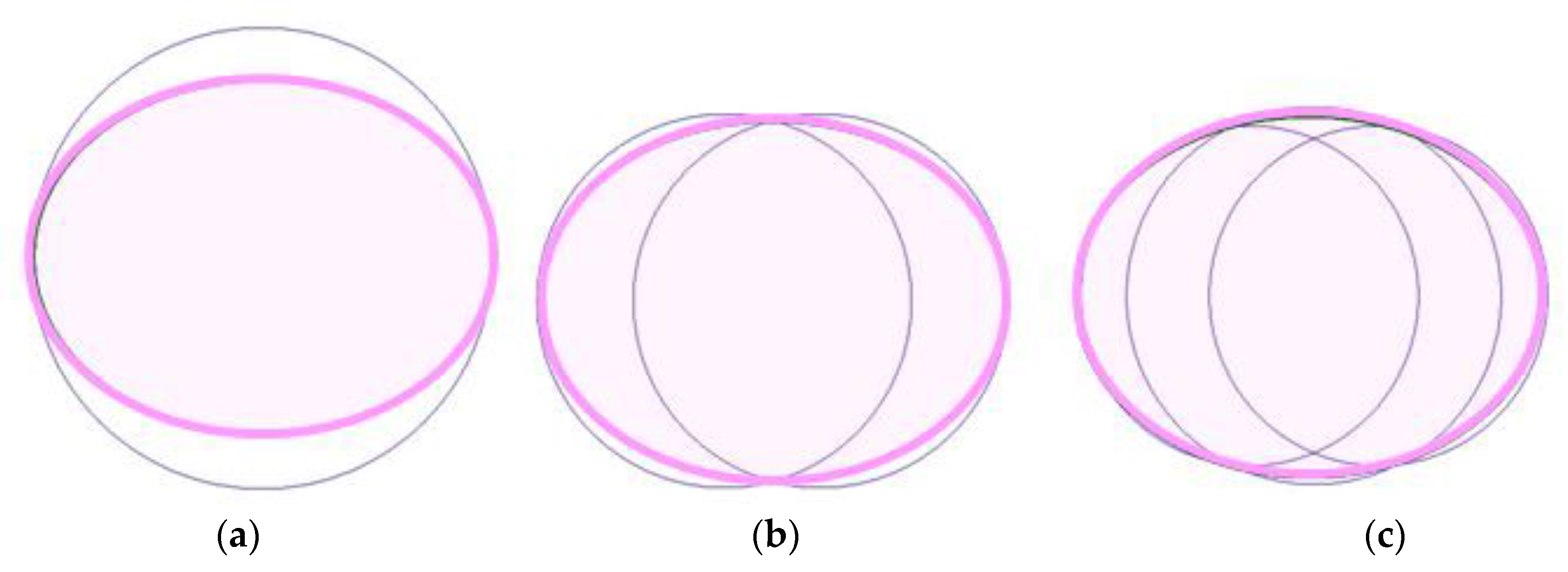
The ellipse with semi-axes 1.3, 1 is given.
- (a)
- For , the solution with one covering circle is presented in Figure 5a:
- (b)
- For , the solution with an even number of covering circles is shown in Figure 5b:{0.265385,−0.265385}, and{1.034615, 1.034615}.
- (c)
- For , the solution with an odd number of covering circles is given in Figure 5c:{0.357061, −0.357061, 0.000},{0.942939, 0.942939, 1.040356}.
Instance 2.
The ellipsewith semi-axes2.3,1 is given and.
- (a)
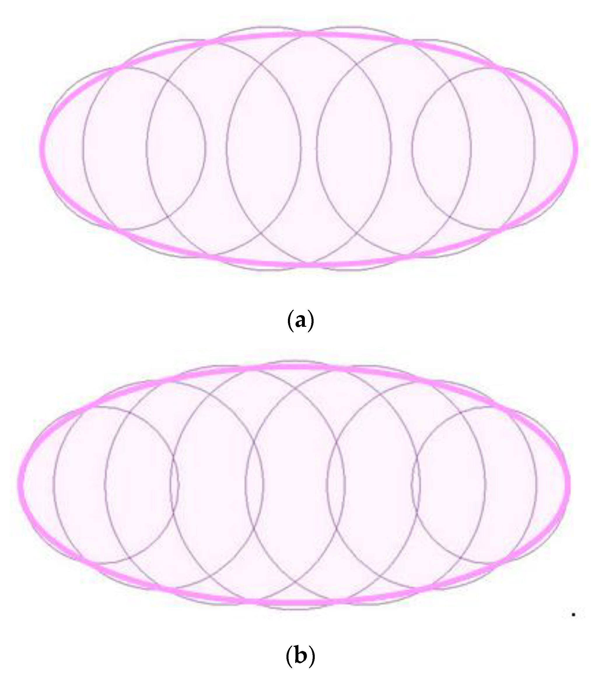
- The optimized cover with an even number of circles is presented in Figure 6a:{1.596217, −1.596217, 1.008362, −1.008362, 0.344754, −0.344754},{0.703783, 0.703783, 0.942524, 0.942524 1.057759, 1.057759}.
- (b)
- The optimized cover with an odd number of circles is shown in Figure 6b:{1.638879, −1.638879, 1.146544, −1.146544, 0.589831, −0.589831, 0.0000},{0.661121, 0.661121, 0.883641, 0.883641, 1.011495, 1.011495, 1.053720}.
Instance 3.
The spheroidwith semi-axes1.9,1 is given and.
- (a)
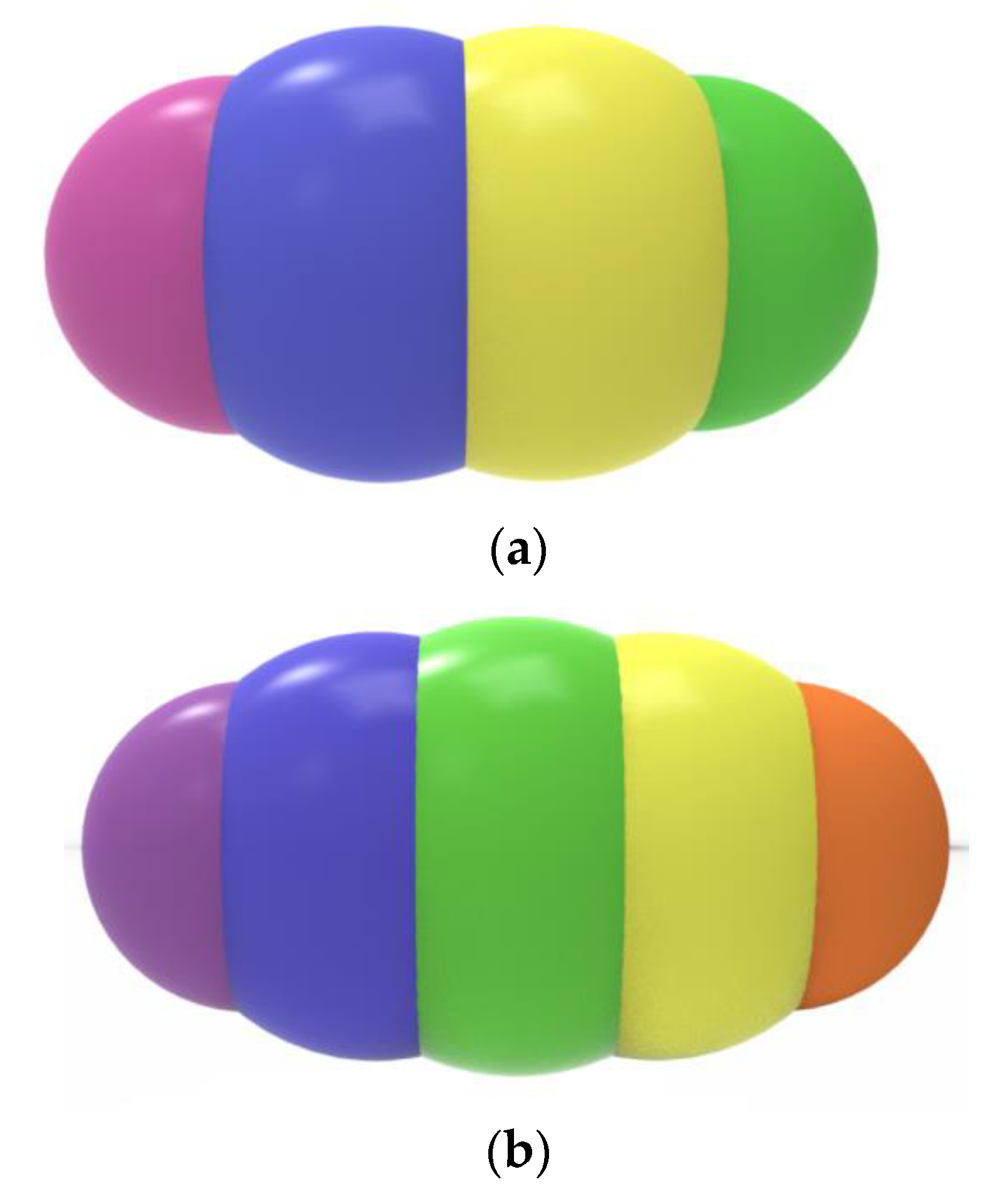
- The optimized cover with an even number of spheres is presented in Figure 7a:{1.054209, −1.054209, 0.367367, −0.367367},{0.845791, 0.845791, 1.065344, 1.065344}.
- (b)
- The optimized cover (for2) with an odd number of spheres is shown in Figure 7b:{1.229404, −1.229404, 0.644245, −0.644245, 0.0000},{0.770596, 0.770596, 0.996786, 0.996786, 1.070009}.
Instance 4.
The spheroidwith semi-axes2,1 is given and.
The optimized cover with an odd number of spheres is presented in Figure 8:
{0.000000, 0.366202, 0.721511, 1.055358, 1.357813, −0.366202, −0.721511, −1.055358, −1.357813},{1.022435, 0.999666, 0.930939, 0.814240, 0.642187, 0.999666, 0.930939, 0.814240, 0.642187}.
Instance 5.
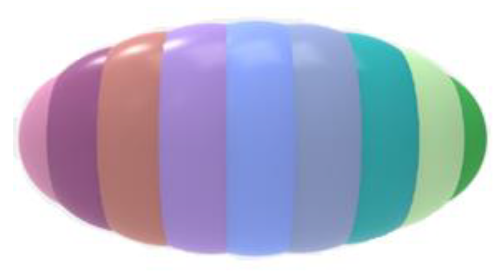
The spheroidwith semi-axes10,1 is given and.
The optimized cover with an odd number of spheres is shown in Figure 9:
{0.000000, 1.395933, 2.764207, 4.077711, 5.310411, 6.437857, 7.437658, 8.289887, 8.977362, 9.485512, 9.798415, −1.395933, −2.764207, −4.077711, −5.310411, −6.437857, −7.437658, −8.289887, −8.977362, −9.485512, −9.798415,},{1.223518, 1.211410, 1.175328, 1.115988, 1.034567, 0.932687, 0.812378, 0.676054, 0.526503, 0.367023, 0.203604, 1.211410, 1.175328, 1.115988, 1.034567, 0.932687, 0.812378, 0.676054, 0.526503, 0.367023, 0.203604}.
5. Conclusions
The problem of optimized multi-spherical covering for spheroids is introduced. This problem is motivated by the packing non-spherical particles arising in naturals sciences and engineering. The simple heuristic approach is proposed to construct an optimized covering, providing a reasonable balance between the number of spheres and the error of approximation. Computational experiments indicate that the proposed approach constructs good feasible coverings very fast: in less than a second. The multi-spherical approximations obtained in the paper provide a basis for fast optimized packing spheroids in different containers, using algorithms proposed, e.g., in [30,31,32]. The two-stage scheme presented in Section 2 can be applied for the general optimized multi-spherical covering. An extension of the covering approach to the case of more complex objects [33,34,35,36] is an interesting direction for the future research. Some results on this topic are on the way.
Author Contributions
Investigation, A.P., T.R., I.L., J.A.M.-S.; Methodology, A.P., T.R., I.L., J.A.M.-S.; Project administration, T.R., I.L.; Writing—original draft, T.R., I.L.; Writing—review and editing, T.R., I.L.; Programming algorithms, A.P.; Numerical experimentation, A.P., T.R. All authors have read and agreed to the published version of the manuscript.
Funding
This research received no external funding.
Acknowledgments
The authors would like to thank anonymous referees for careful reading the paper and constructive comments. The first two authors were partially supported by the “Program for the State Priority Scientific Research and Technological (Experimental) Development of the Department of Physical and Technical Problems of Energy of the National Academy of Sciences of Ukraine” (#6541230).
Conflicts of Interest
The authors declare no conflict of interest.
Appendix A
We would like to thank the anonymous referee for pointing out that the explicit expressions can be obtained for rk, and in our algorithm at Stage 1.
The parameters have been derived based on constructions proposed in [28].
- 1.
- Deriving.
Observe that the point belongs to the coordinate axis OX for , while the point belongs to the frontier of the ellipse.
Since , then for and , , , , .
The tangent point , belongs to the frontier of the ellipse.
Since , then and thus .
Here we used
Therefore at the k-th iteration.
- 2.
- Deriving.
The tangent point is defined from the system
Therefore , , and thus
, .
- 3.
- Deriving.
From the system at Step2 we have .
Therefore , and thus , .
References
- Bernal, J.D. A geometrical approach to the structure of liquids. Nature 1959, 183, 141–147. [Google Scholar] [CrossRef]
- Stillinger, F.H.; Marzio, E.A.D.; Kornegay, R.L. Systematic approach to explanation of the rigid disk phase transition. J. Chem. Phys. 1964, 40, 1564–1576. [Google Scholar] [CrossRef]
- Makse, H.; Kurchan, J. Testing the thermodynamic approach to granular matter with a numerical model of a decisive experiment. Nature 2002, 415, 614–617. [Google Scholar] [CrossRef] [PubMed]
- Costamagna, P.; Costa, P.; Antonucci, V. Micro-modelling of solid oxide fuel cell electrodes. Electrochim. Acta 1998, 43, 375–394. [Google Scholar] [CrossRef]
- Zerhouni, O.; Tarantino, M.G.; Danas, K. Numerically-aided 3D printed random isotropic porous materials approaching the Hashin-Shtrikman bounds. Compos. Part B Eng. 2019, 156, 344–354. [Google Scholar] [CrossRef] [Green Version]
- Gan, J.; Yu, A.; Zhou, Z. DEM simulation on the packing of fine ellipsoids. Chem. Eng. Sci. 2016, 156, 64–76. [Google Scholar] [CrossRef]
- Gately, R.D.; Panhuis, M. Filling of carbon nanotubes and nanofibres. Beilstein J. Nanotechnol. 2015, 6, 508–516. [Google Scholar] [CrossRef] [Green Version]
- Ustach, V.; Faller, R. The raspberry model for protein-like particles: Ellipsoids and confinement in cylindrical pores. Eur. Phys. J. Spec. Top. 2016, 225, 1643–1662. [Google Scholar] [CrossRef] [Green Version]
- Wang, X.; Zhao, L.; Fuh, J.Y.H.; Lee, H.P. Effect of Porosity on Mechanical Properties of 3D Printed Polymers: Experiments and Micromechanical Modeling Based on X-ray Computed Tomography Analysis. Polymers 2019, 11, 1154. [Google Scholar] [CrossRef] [Green Version]
- Li, C.X.; Zou, R.P.; Pinson, D.; Yu, A.B.; Zhou, Z.Y. An experimental study of packing of ellipsoids under vibrations. Powder Technol. 2020, 361, 45–51. [Google Scholar] [CrossRef]
- Akeb, H. A Look-Ahead-Based Heuristic for Packing Spheres into a Bin: The Knapsack Case. Procedia Comput. Sci. 2015, 65, 652–661. [Google Scholar] [CrossRef] [Green Version]
- Stoyan, Y.; Scheithauer, G.; Yaskov, G. Packing Unequal Spheres into Various Containers. Cybern. Syst. Anal. 2016, 52, 419–426. [Google Scholar] [CrossRef]
- Stetsyuk, P.; Romanova, T.; Scheithauer, G. On the global minimum in a balanced circular packing problem. Optim. Lett. 2016, 10, 1347–1360. [Google Scholar] [CrossRef]
- Hifi, M.; Yousef, L. A local search-based method for sphere packing problems. Eur. J. Oper. Res. 2019, 274, 482–500. [Google Scholar] [CrossRef]
- Litvinchev, I.; Infante, L.; Ozuna, L. Packing circular-like objects in a rectangular container. J. Comput. Syst. Sci. Int. 2015, 54, 259–267. [Google Scholar] [CrossRef]
- Torres-Escobar, R.; Marmolejo-Saucedo, J.A.; Litvinchev, I. Binary monkey algorithm for approximate packing non-congruent circles in a rectangular container. Wirel. Netw. 2018. [Google Scholar] [CrossRef]
- Bertei, A.; Chueh, C.-C.; Pharoah, J.G.; Nicolella, C. Modified collective rearrangement sphere-assembly algorithm for random packings of nonspherical particles: Towards engineering applications. Powder Technol. 2014, 253, 311–324. [Google Scholar] [CrossRef]
- Kallrath, J. Packing ellipsoids into volume-minimizing rectangular boxes. J. Glob. Optim. 2017, 67, 151–185. [Google Scholar] [CrossRef]
- Birgin, E.; Lobato, R. A matheuristic approach with nonlinear subproblems for large-scale packing of ellipsoids. Eur. J. Oper. Res. 2019, 272, 447–464. [Google Scholar] [CrossRef]
- Kampas, F.; Castillo, I.; Pintér, J. Optimized ellipse packings in regular polygons. Optim. Lett. 2019, 13, 1583–1613. [Google Scholar] [CrossRef]
- Pankratov, A.; Romanova, T.; Litvinchev, I. Packing ellipses in an optimized rectangular container. Wirel. Netw. 2018. [Google Scholar] [CrossRef]
- Pankratov, A.; Romanova, T.; Litvinchev, I. Packing ellipses in an optimized convex polygon. J. Glob. Optim. 2019, 75, 495–522. [Google Scholar] [CrossRef]
- Romanova, T.; Stoyan, Y.; Pankratov, A.; Litvinchev, I.; Avramov, K.; Chernobryvko, M.; Yanchevskyi, I.; Mozgova, I.; Bennell, J. Optimal layout of ellipses and its application for additive manufacturing. Int. J. Prod. Res. 2019. [Google Scholar] [CrossRef]
- Litvinchev, I.; Infante, L.; Ozuna, L. Approximate Circle Packing in a Rectangular Container: Integer Programming Formulations and Valid Inequalities. In Lecture Notes in Computer Science; Gonzalez-Ramirez, R.G., Ed.; Springer: Berlin/Heidelberg, Germany, 2014; Volume 8760, pp. 47–60. [Google Scholar]
- Jones, D.R. A fully general, exact algorithm for nesting irregular shapes. J. Glob. Optim. 2014, 59, 367–404. [Google Scholar] [CrossRef]
- Rocha, P.; Gomes, A.M.; Rodrigues, R.; Toledo, F.M.B.; Andretta, M. Constraint aggregation in non-linear programming models for nesting problems. In Computational Management Science: State of the Art 2014; Fonseca, J.R., Weber, G.-W., Telhada, J., Eds.; Springer International Publishing: Cham, Switzerland, 2016; pp. 175–180. [Google Scholar]
- Yuan, Y.; Liu, L.; Deng, W.; Li, S. Random-packing properties of spheropolyhedra. Powder Technol. 2019, 351, 186–194. [Google Scholar] [CrossRef]
- Birgin, E.; Bustamante, L.; Callisaya, H.; Martnez, J. Packing circles within ellipses. Int. Trans. Oper. Res. 2013, 20, 365–389. [Google Scholar] [CrossRef] [Green Version]
- Wachter, A.; Biegler, L. On the implementation of an interior-point filter line-search algorithm for large-scale nonlinear programming. Math. Programm. 2006, 106, 25–57. [Google Scholar] [CrossRef]
- Stoyan, Y.; Romanova, T. Mathematical models of placement optimisation: Two- and three-dimensional problems and applications. In Modeling and Optimization in Space Engineering; Fasano, G., Pintér, J., Eds.; Springer Optimization and its Applications: New York, NY, USA, 2013; Volume 73, pp. 363–388. [Google Scholar]
- Stoyan, Y.; Pankratov, A.; Romanova, T. Cutting and packing problems for irregular objects with continuous rotations: Mathematical modeling and nonlinear optimization. J. Oper. Res. Soc. 2016, 67, 786–800. [Google Scholar] [CrossRef]
- Romanova, T.; Bennell, J.; Stoyan, Y.; Pankratov, A. Packing of concave polyhedra with continuous rotations using nonlinear optimization. Eur. J. Oper. Res. 2018, 268, 37–53. [Google Scholar] [CrossRef]
- Kiseleva, E.M.; Lozovskaya, L.I.; Timoshenko, E.V. Solution of continuous problems of optimal covering with spheres using optimal set-partition theory. Cybern. Syst. Anal. 2009, 45, 421–437. [Google Scholar] [CrossRef]
- Scheithauer, G.; Stoyan, Y.G.; Romanova, T.; Krivulya, A. Covering a polygonal region by rectangles. Comput. Optim. Appl. Springer Neth. 2011, 48, 675–695. [Google Scholar]
- Yakovlev, S.; Kartashov, O.; Komyak, V.; Shekhovtsov, S.; Sobol, O.; Yakovleva, I. Modeling and simulation of coverage problem in geometric design systems. In Proceedings of the 15th International Conference on the Experience of Designing and Application of CAD Systems, CADSM 2019, Lviv, Ukraine, 26 February–2 March 2019; pp. 20–23. [Google Scholar]
- Torres-Escobar, R.; Marmolejo-Saucedo, J.A.; Litvinchev, I.; Vasant, P. Monkey algorithm for packing circles with binary variables. In Intelligent Computing & Optimization. ICO 2018; Vasant, P., Zelinka, I., Weber, G.-W., Eds.; Springer International Publishing: Cham, Switzerland, 2019; Volume 866, pp. 547–559. [Google Scholar]
Figure 1.
The center of the first approximating circle: (a) for odd circular covering and (b) for even circular covering.
Figure 1.
The center of the first approximating circle: (a) for odd circular covering and (b) for even circular covering.

Figure 2.
Illustrations of the first and the second iterations of the algorithm for Stage 1: (a) the first iteration; (b) the second iteration.
Figure 2.
Illustrations of the first and the second iterations of the algorithm for Stage 1: (a) the first iteration; (b) the second iteration.

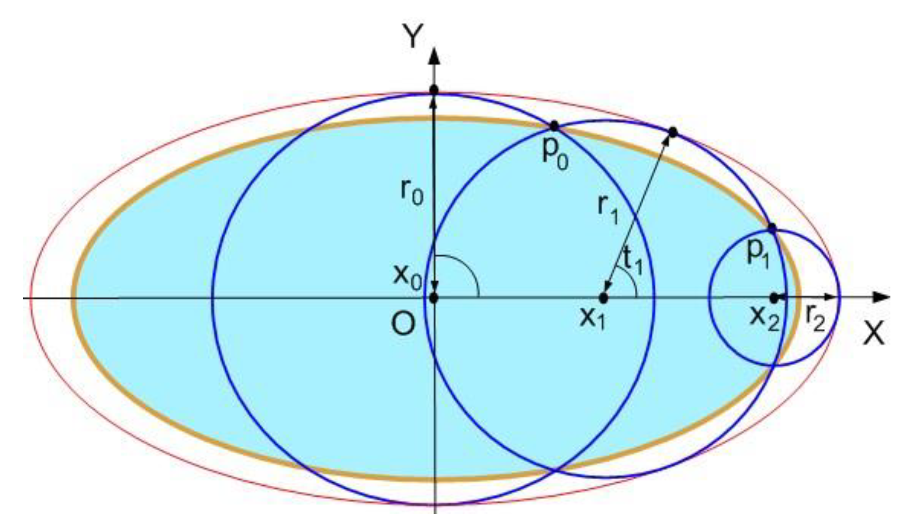
Figure 3.
Illustration of the solution obtained at Step 6 of the last iteration of the algorithm for Stage 1.
Figure 3.
Illustration of the solution obtained at Step 6 of the last iteration of the algorithm for Stage 1.

Figure 4.
Illustration of Stage 2.

Figure 5.
The optimized cover of the ellipse : (a) by circle; (b) by circles; and (c) by circles.

Figure 6.
The optimized cover of the ellipse : (a) by circles; (b) by circles.

Figure 7.
The optimized cover of the spheroid : (a) by spheres; (b) by spheres.

Figure 8.
The optimized cover of the spheroid by spheres.

Figure 9.
The optimized cover of the spheroid by spheres.

© 2020 by the authors. Licensee MDPI, Basel, Switzerland. This article is an open access article distributed under the terms and conditions of the Creative Commons Attribution (CC BY) license (http://creativecommons.org/licenses/by/4.0/).
Share and Cite
MDPI and ACS Style
Pankratov, A.; Romanova, T.; Litvinchev, I.; Marmolejo-Saucedo, J.A. An Optimized Covering Spheroids by Spheres. Appl. Sci. 2020, 10, 1846. https://doi.org/10.3390/app10051846
AMA Style
Pankratov A, Romanova T, Litvinchev I, Marmolejo-Saucedo JA. An Optimized Covering Spheroids by Spheres. Applied Sciences. 2020; 10(5):1846. https://doi.org/10.3390/app10051846
Chicago/Turabian StylePankratov, Alexander, Tatiana Romanova, Igor Litvinchev, and Jose Antonio Marmolejo-Saucedo. 2020. "An Optimized Covering Spheroids by Spheres" Applied Sciences 10, no. 5: 1846. https://doi.org/10.3390/app10051846
Note that from the first issue of 2016, this journal uses article numbers instead of page numbers. See further details here.