Turboelectric Uncertainty Quantification and Error Estimation in Numerical Modelling

Abstract

Turboelectric systems can be considered complex systems that may comprise errors and uncertainty. Uncertainty quantification and error estimation processes can, therefore, be useful in achieving accurate system parameters. Uncertainty quantification and error estimation processes, however, entail some stages that provide results that are more positive. Since accurate approximation and power optimisation are crucial processes, it is essential to focus on higher accuracy levels. Integrating computational models with reliable algorithms into the computation processes leads to a higher accuracy level. Some of the current models, like Monte Carlo and Latin hypercube sampling, are reliable. This paper focuses on uncertainty quantification and error estimation processes in turboelectric numerical modelling. The current study integrates the current evidence with scholarly sources to ensure the incorporation of the most reliable evidence into the conclusions. It is evident that studies on the current subject began a long time ago, and there is sufficient scholarly evidence for analysis. The case study used to obtain this evidence is NASA N3-X, with three aircraft conditions: rolling to take off, cruising and taking off. The results show that the electrical elements in turboelectric systems can have decent outcomes in statistical analysis. Moreover, the risk of having overload branches is up to 2% of the total aircraft operation lifecycle, and the enhancement of the turboelectric system through electrical power optimisation management could lead to higher performance.

1. Introduction

Uncertainty is a common occurrence in engineering systems. It entails the process of accurately computing the extent to which a mathematical model can describe the relevant physics. It also concerns the impact of model uncertainty, which is either parametric or structural, on the outputs of the model. Error estimation, on the other hand, entails the task of determining the accuracy of a particular numerical technique in its approximation of a given output. It is also common in engineering systems due to there being several mechanical factors that are involved in their composition. A turboelectric aircraft utilises combustible fuel for the storage of energy, but it also uses electric power transmission, and not mechanical transmission, to drive the propulsors [1,2]. A turboelectric design is just a different configuration or architecture for hybrid-electric or all-electric models. Turboelectric models are hybrids that lack batteries [3]. Uncertainty quantification and the error estimation process, however, entail the use of various techniques for different types of uncertainties.

The need for sampling study in the turboelectric system presented to find the accuracy of the output approximation of the mathematical model which the study will result in error estimation for the numerical method used [4,5]. Moreover, the sampling method been used to optimise turboelectric propulsion system with the two objectives electrical power and efficiency.

This paper studies the uncertainty in turboelectric distributed propulsion (TeDP) systems and estimates the error in their utilisation. In addition, it fills in the gap of quantitative risk analysis in numerical modelling for futuristic propulsion systems.

2. Network Model Method

A high-level set of electrical network architectures are designed to obtain the optimal power flow within the required post-process results. At the start of the designed network, the input data are considered first. These data are the values of the electrical parameters generated or intended for propulsion design. Then, these values are applied to Kirchhoff’s and Ohm’s laws. The three principle laws are

• Kirchhoff’s current law

G. R. Kirchhoff, a German scientist, proposed a fundamental law, known as Kirchhoff’s current law (KCL). This law states that the sum of the currents at an electric node needs to be zero, which is defined formally in [6,7]:

$${\displaystyle \sum }_{n=1}^N{i}_n=0$$

• Kirchhoff’s voltage law

Voltage is the motion of electric charge between two points and can be defined as the total work per unit charge. Furthermore, the voltage was defined as a unit of energy per charge by the Italian physicist Alessandro Volta as part of his contribution with regard to the electric battery:

$$volt=\frac{joule\left(energy\right)}{coulomb\left(electriccharge\right)}$$

After several experimental works on voltage, Kirchhoff proposed his second law called Kirchhoff’s voltage law (KVL) based on the principle that no loss in energy can occur in an electric circuit. This implies that the sum of all voltage sources must be equal to the sum of load voltages, which results in a total of zero for any closed circuit, as in [6,7]:

$${\displaystyle \sum }_{n=1}^N{v}_n=0$$

• Ohm’s law

Material properties are the main factors that affect the resistance when electric current flows through the conductors or circuit elements. This resistance during the current flow in the circuit elements can be considered as energy loss, which may be converted to the form of heat. According to Ohm’s law, which deals with an ideal resistor,

$$V=IR$$

As R is the value of resistance with the unit Ohm (Ω), it can be defined as the voltage across an element divided by the current flow through it:

$$\Omega =\frac{V}{A}$$

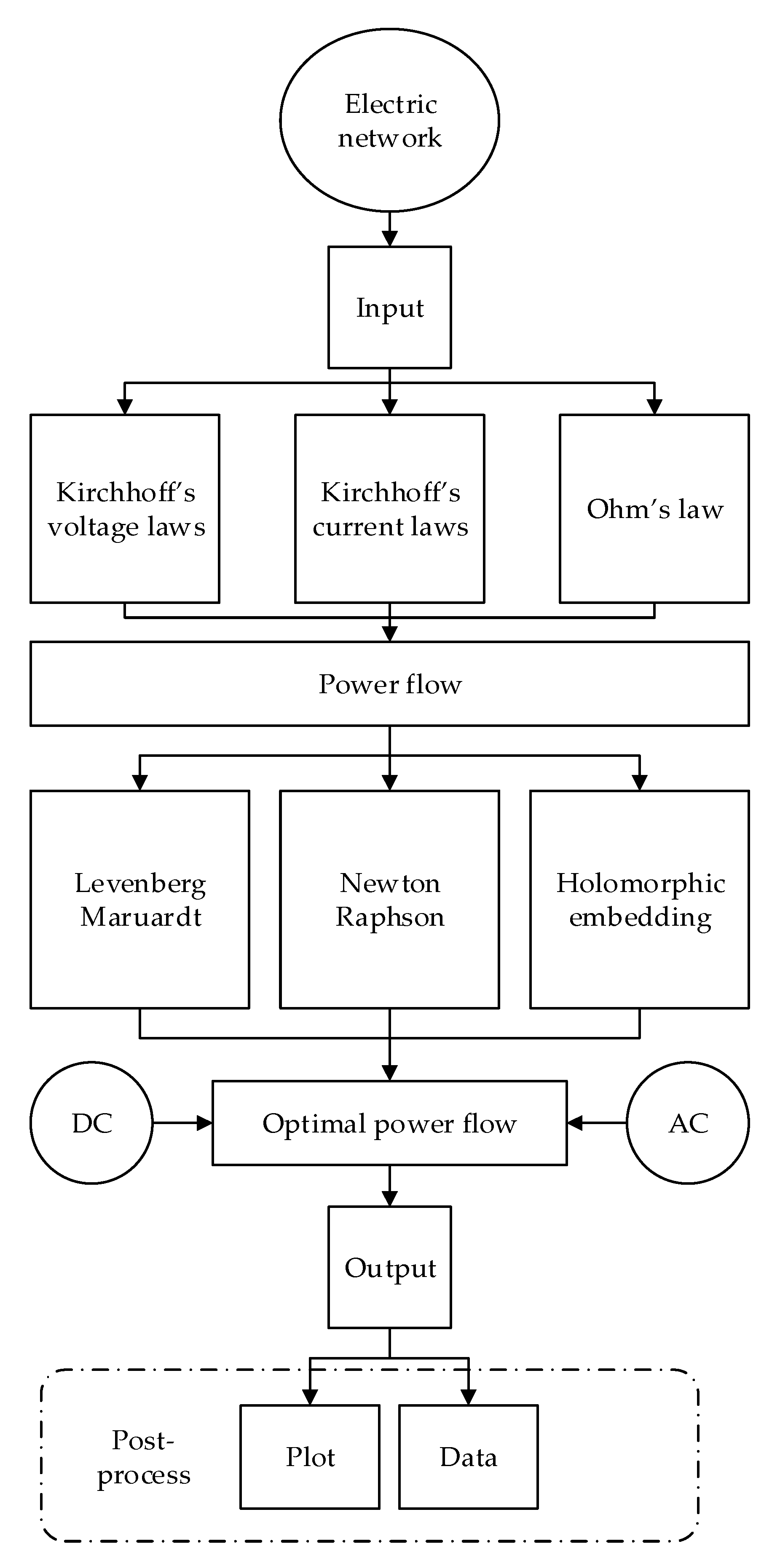
To optimise the power flow in this stage, three methods were included within the module, as described below:

• Levenberg–Marquardt

In the early 1960s, the Levenberg–Marquardt algorithm (LMA) was introduced to solve the nonlinear least-squares problem. It minimises the sum of squares errors using a sequence of updates to the parameter values between the measured data points and the fit parameterised function. Moreover, the nonlinear problem implies that the parameters of the fit function are not linear. The algorithm by itself consists of two methods, combination and calculation, depending on the optimal value: the gradient descent method, which updates the parameters in the steepest-descent direction, and the Gauss–Newton method, which assumes that the least-squares function is locally quadratic by determining its minimum. Thus, when the optimal values for the parameters are distant, then the LMA adopts the gradient descent method, whereas, when the optimal values for the parameters are close to each other, then the LMA adopts the Gauss–Newton method [8,9].

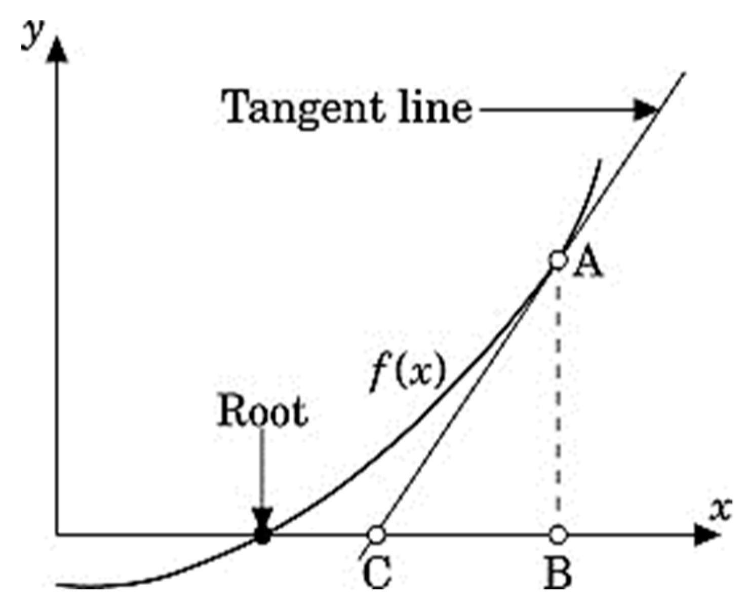
• Newton Raphson

This method was proposed in 1685 by John Wallis as a root-finding approximation using a straight tangent [10,11]. Figure 1 illustrate Newton-Raphson method.

• Holomorphic embedding

In 2012, Antonio Trias proposed the holomorphic embedding load flow method (HELM) as a novel non-iterative and non-initial value algorithm. It uses the techniques of complex and deterministic analysis. In brief, the HELM mechanism comprises the following steps [13,14]:

• Find a suitable complex holomorphic embedding with the help of a complex parameter.
• Calculate the power series using a sequence of linear systems that yield the coefficients progressively.
• Determine the solution of the complex parameter as the analytical continuation of the power series via Pad’e Approximants.

Figure 2 depicts these methods and illustrates the modelled electric network architecture for the numerical simulation software to solve hybrid and turboelectric implementation.

2.1. Generator

The generator is modelled as a function in a specific buss. For generator $x$, the function is

$$G\left(x\right)=P\left(x\right)+jq\left(x\right)$$

which combines the active and the reactive powers for the generator in the specific buss as follows:

$$Generatorpower\left(buss\right)=Activepower\left(buss\right)+Reactivepower\left(buss\right)$$

Then, the connection between the generators using a matrix and the buss is expressed as follows:

$$Generatorbuss\left(x\right)=Matrix\left(x\right)\times Generator\left(x\right)$$

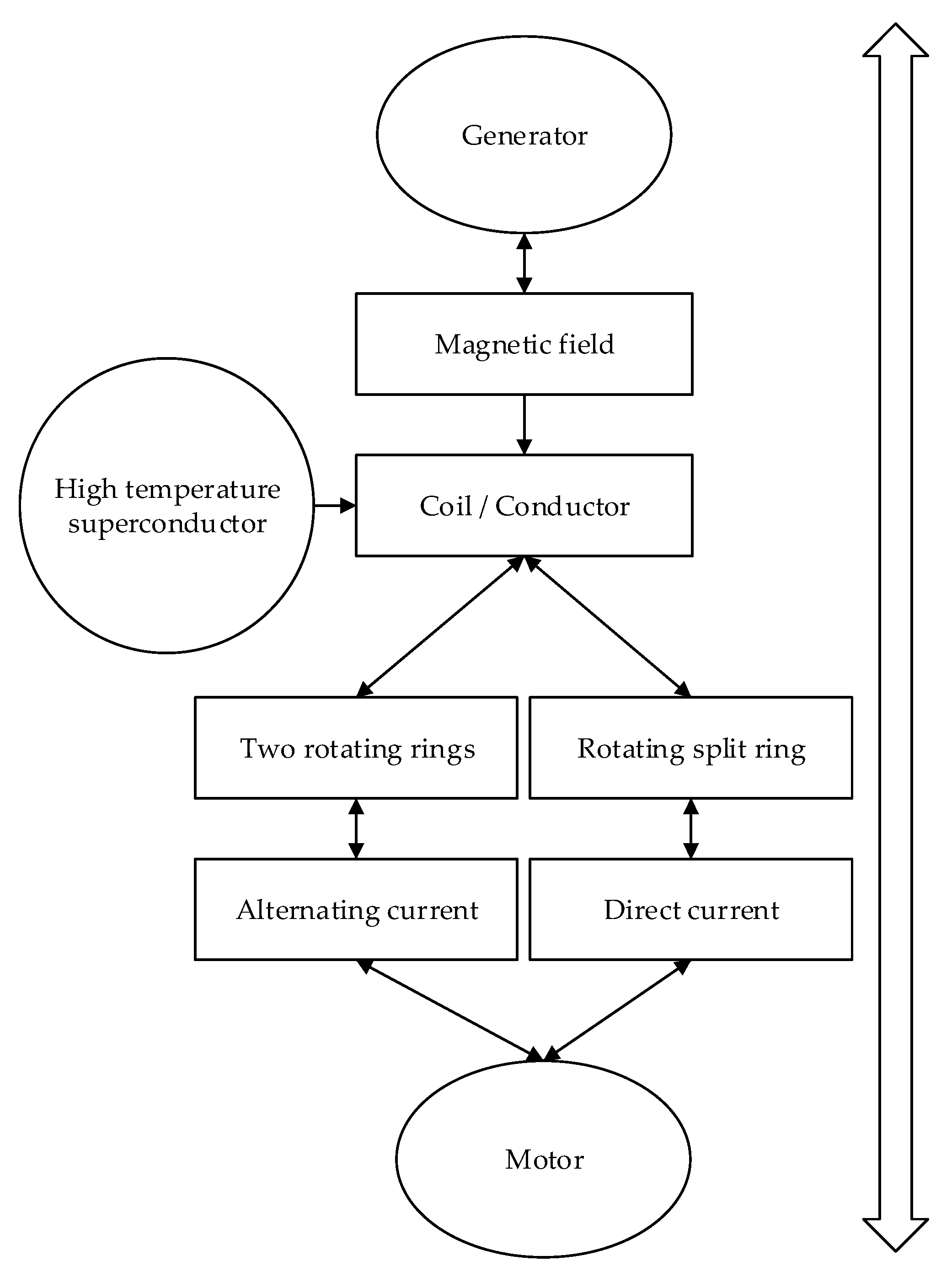
As per the basic generator concept, magnetic power is the hidden power that converts mechanical power into electrical power. Through the rotation of the components, a magnetic field is generated, and the conductor or the coil absorbs these effects to generate electricity. Therefore, depending on the conductor type (material specifications), in the event of high-temperature superconductivity, the efficiency of the conductance varies with temperature limitations. The generator can be of two types: two rotating rings or a rotating split ring, depending on the type of generated current. In the case of the rotating split ring, the output is a direct current, whereas, in the case of two rotating rings, the output is alternating current. Figure 3 depicts the relation between the generator-modelled prototypes, the inverse of which is the motor prototype.

The following are the Equations (1)–(14) developed to determine the generator model steps and calculation for the range of voltage, resistance and load [15,16,17]:

$$Rotationrate=\frac{Powershaft}{Torque}$$

(1)

$$Revolutionsperminute=\frac{Rotationrate}{\raisebox{1ex}{$\pi $}\!\left/ \!\raisebox{-1ex}{$30$}\right.}$$

(2)

$$Speedconstant\left(Radian\right)=\frac{Speedconstant\left(Revolutionsperminute\right)}{\raisebox{1ex}{$\pi $}\!\left/ \!\raisebox{-1ex}{$30$}\right.}$$

(3)

$$Torqueconstant\left(Radian\right)=Speedconstant\left(Radian\right)$$

(4)

$$Generatorvoltage=\frac{Rotationrate}{Speedconstant\left(Radian\right)}$$

(5)

$$Current=Torque\times Torqueconstant\left(Radian\right)$$

(6)

$$Voltage=Generatorvoltage+Resistance\times Current$$

(7)

$$Hightemperaturesuperconductorefficiency=\frac{Totalcurrenttemperature-Temperaturelimit}{Temperaturelimit}$$

(8)

$$Electricpower=Voltage\times Current$$

(9)

If high-temperature superconductor > 0,

$$\begin{array}{ll}generatorefficiency& =\frac{Electricpower}{Powershaft}\\ & -Hightemperaturesuperconductorefficiency\times 100.\end{array}$$

(10)

Else,

$$Generatorefficiency=\frac{Electricpower}{Powershaft}$$

(11)

Loss determination:

$$Losspower=Shaftpower-Electricpower$$

(12)

$$Losspower=Windagefraction+Materialsresistance$$

(13)

If high-temperature superconductor ≤ 0, materials resistance = 0

$$Losspower=Windagefraction$$

(14)

2.2. Motor

The motor is modelled as a constant power load with a specified quantity of active and reactive power consumed at a buss. For buss $x$, the load is

$$M\left(x\right)=P\left(x\right)+jq\left(x\right)$$

which combines the active and reactive powers for the motor in the specific buss as follows:

$$Motorpower\left(buss\right)=Activepower\left(buss\right)+Reactivepower\left(buss\right)$$

Moreover, as mentioned in Figure 3, the motor model prototype is the inverse of the generator prototype.

The following are the equations (15-28) developed to determine the motor model steps and calculation for the range of voltage, resistance and load [15,16,17]:

$$Motorvoltage=Voltage-Resistance\times Current$$

(15)

$$Speedconstant\left(Radian\right)=Torqueconstant\left(Radian\right)$$

(16)

$$Tourque=\frac{Current}{Torqueconstant\left(Radian\right)}$$

(17)

$$Rotationrate=Motorvoltage\times Speedconstant\left(Radian\right)$$

(18)

$$Speedconstant\left(Revolutionsperminute\right)=Speedconstant\left(Radian\right)\times \pi ⁄30$$

(19)

$$Rotationrate=Revolutionsperminute\times \raisebox{1ex}{$\pi $}\!\left/ \!\raisebox{-1ex}{$30$}\right.$$

(20)

$$Powershaft=Rotationrate\times Torque$$

(21)

$$Electricpower=Voltage\times Current$$

(22)

$$Hightemperaturesuperconductorefficiency=\frac{Totalcurrenttemperature-Temperaturelimit}{Temperaturelimit}$$

(23)

If high-temperature superconductor > 0,

$$\begin{array}{ll}Motorefficiency& =\frac{Powershaft}{Electricpower}\\ & -Hightemperaturesuperconductorefficiency\times 100\end{array}$$

(24)

Else,

$$Motorefficiency=\frac{PowerShaft}{Electricpower}$$

(25)

Loss determination:

$$Losspower=Electricpower-Shaftpower$$

(26)

$$LossPower=WindageFraction+MaterialsResistance$$

(27)

If high-temperature superconductor ≤ 0, materials resistance = 0

$$LossPower=WindageFraction$$

(28)

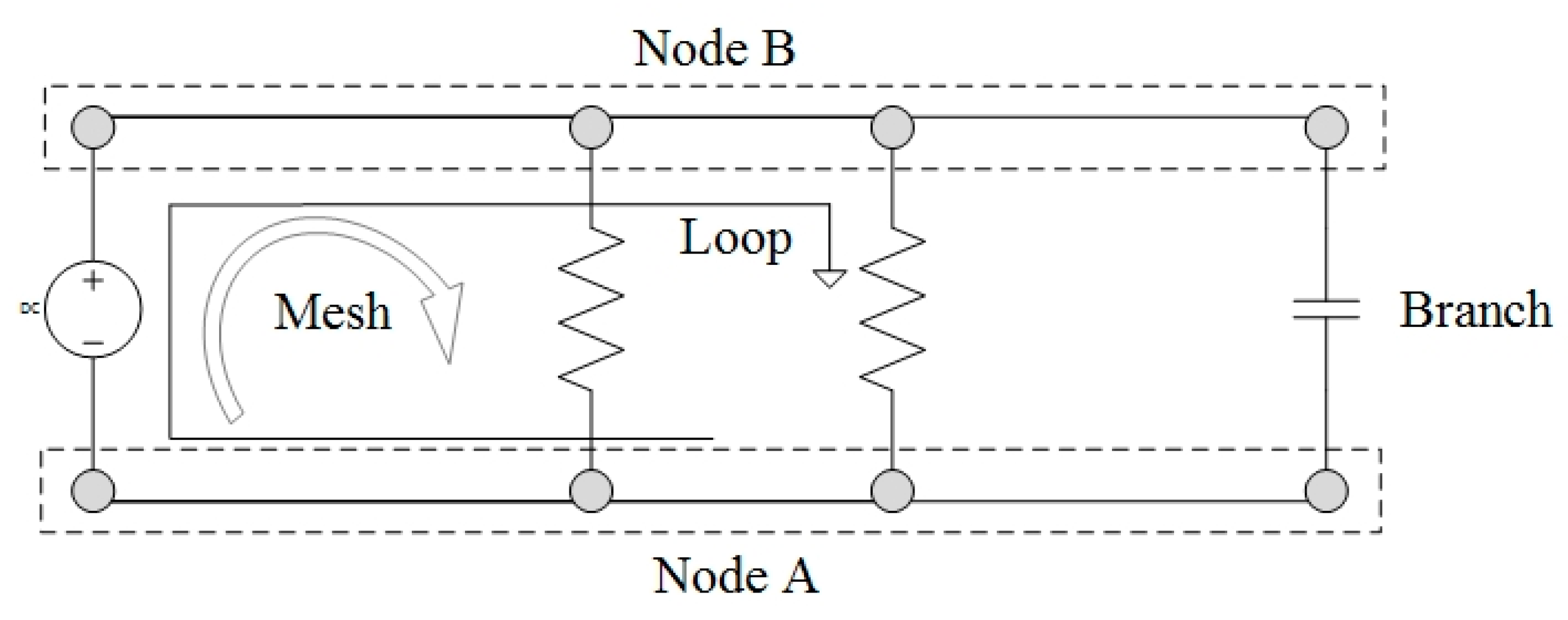
2.3. Circuit

The electric circuit is modelled as a standard electric principle to represent nodes and branches. To illustrate the electric circuit structure, Figure 4 depicts an electric branch, node, loop and mesh. This circuit can be used in multi-circuits as the scale of the data examined by means of object ordinated capability.

Node:

The node model helps to analyse and calculate the electrical circuit parameters by applying KCL in each node to obtain the simultaneous equations, whereas the mesh model needs to apply KVL to solve the electrical parameters [18].

Buss:

The buss is a part of the node configuration, which represents the wiring connection between the power sources, loads and electrical converters. It carries the reactive power, voltage and the resistance of the link depending on the material or the length of the bus.

Branch:

The branch model is a median between different nodes and has the ability to transfer the power type and size.

3. Impact of Model Uncertainty

Apparently, during the development of numerical models, uncertainty quantification tasks can lead to a suitable framework for the allocation of computational resources. They most often lead to an efficient investigation in activity role model standardisation and a robust design [19]. During turboelectric numerical modelling, several uncertainties can emerge due to assumptions associated with unavoidable circumstances. It is crucial to account for those uncertainties. Uncertainty quantification can enable the prediction of the effects of the sources of uncertainties on numerical models and the effects of the inherent assumptions they make about the models. Uncertainty quantification strategies affect modelling processes because they can enhance the optimisation processes and sound design. The process of uncertainty quantification entails processes, such as effect screening, forward uncertainty propagation, parametric studies and sensitivity analysis.

In modelling and simulation, however, the uncertainty quantification process typically entails the utilisation of parametric studies. In that regard, the uncertainty sources refer to the sources delineated by the model parameters. In turboelectric numerical modelling, aspects like the crashworthiness of an aircraft constitute a possible area of beneficial research, but there is a high level of uncertainty [19]. The uncertainty associated with the airworthiness of an aircraft increases the risk of an accident because of the inability to obtain reliable results. Uncertainty also affects the predictability of the possible outcomes. In this regard, it can amount to a negative impact due to cause inaccuracies in selecting the best action to take to enhance the safety in the utilisation of an aircraft. For example, the aerospace industry tends to replace liquid fuel with batteries because liquid fuel tends to worsen the situation when a crash occurs.

Model uncertainty cannot help in predicting the possible outcomes of the numerical modelling process of a turboelectric system. However, it prevents accurate determination of the sensitivity of input power. In particular, with increased model uncertainty, it becomes difficult to predict the input power of the cryogenic system in an aircraft [20]. Due to the inability to predict the input power, owing to the model uncertainty, it also becomes difficult to determine the mass of the single-stage and two-stage reverse-Brayton cycle cryocoolers (RBCCs) for distributed electrical aerospace propulsion (DEAP). The challenges can also extend to the parameters necessary for the operation of the RBCCs. Inaccurate estimation of the input power and probable effects on the power transmission fluctuations throughout the system make it challenging to predict the correct temperature required for cryocooling power [20].

The effect of model uncertainty is that several crucial parameters become unpredictable and the system can only be operated on the basis of estimates which, in turn, exacerbates the effect of the error. For example, the current-carrying capacity of a superconducting material depends on essential parameters, such as the temperature, current density and magnetic field density. The effect of model uncertainty can, therefore, affect significant measures of aircraft systems. Power optimisation becomes almost unachievable, and this leads to difficulties in producing accurate approximations. Addressing model uncertainty is vital to enabling accurate uncertainty quantification and error estimation in turboelectric numerical modelling. Considering all the parameters is key to an accurate estimation of aircraft operating conditions in turboelectric systems.

4. Accurate Approximation

Computational efforts develop with the increase in the number of random variables used in making accurate approximations of the input. An upsurge of random variables can slightly reduce the accuracy levels due to the associated approximations [21]. The problem tends to increase in the stochastic collocation version. The increase in computational efforts is necessary for enhancing the accuracy of the interpretation of high-dimensional space. In some case studies, the improvement of uncertainty quantification and error estimation processes using computational models is essential. Computational models, similarly to the Bayesian model, which is a statistical model that uses probability for the uncertainty model, can enhance and utilise the approximation optimality and improve the general accuracy level if incorporated with the Monte Carlo algorithm. This can enhance the accuracy, which enables the values to be spread correctly and the sample to be selected correctly, and this is also representative of the intervals across the entire iteration [21,22].

Approximation accuracy is crucial because of the error that the approximations can introduce into the uncertainty quantification process and the turboelectric numerical modelling process. Uncertainty quantification and error estimation processes should be accurate when developing relevant solutions to and representatives of the parameters involved in the turboelectric numerical modelling of an aircraft. During error estimation procedures, it is necessary to ensure those accurate approximations serve as the source of the conclusions that are eventually made.

It is crucial to consider integrating the most representative sample values to achieve an accurate data interpretation. These data determine the effectiveness of the turboelectric numerical modelling process and the way it can address any issues arising in aircraft systems that affect the safety of the aircraft. The uncertainty quantification and error estimation processes should not only indicate the safety or efficiency of the system, but also the cost minimisation process to ensure that a reliable alternative is always available in technical, environmental, or economical terms. The outputs of several approximations simultaneously enable the enhancement of the accuracy and computational efficiency of the model. The simultaneous application of the computational models resembles a mixture of the expert models used in statistical applications. Every approximate solver provides some incomplete data concerning the high-fidelity model. The model undergoes aggregation to achieve the best possible estimate. The more the approximation models are incorporated, the higher the achievable accuracy level. The accuracy of approximation is therefore crucial to the success of the uncertainty quantification process because it determines the accuracy of the turboelectric numerical modelling process. Computational modelling strategies aid in the enhancement of the accuracy of the output results. The more the computational models are used, the greater the chances of achieving higher accuracy levels. Accurate approximation also entails the use of models with reliable algorithms, such as Monte Carlo.

5. Quantitative Risk Analysis

There are several types of quantitative risk analysis methods for error estimation. This research focuses on two types: Monte Carlo and Latin hypercube. These two were chosen because of the advantages that each has in the study of uncertainty. The Latin hypercube algorithm, also known as the memory analysis method, allows for less sampling, which will provide better performance. However, it decreases the computational complexity in the numerical modelling process. On the other hand, Monte Carlo, also known as the memoryless method, enhances the simplicity in numerical modelling, allowing for the processing of more samples, which increases the performance.

5.1. Monte Carlo

The Monte Carlo technique is a standard method used in uncertainty quantification because it is simple and generates the desired or accurate statistical results. This technique, however, has a low computational cost, which tends to be reasonable in most cases [23]. Since the Monte Carlo algorithm is parallelisable, this can allow the Monte Carlo method to be utilised in simulations in which the computation of one realisation is inexpensive. The idea of the Monte Carlo method is to produce several samples of the random factors based on their distributions. All samples outline a deterministic problem, resolved using a deterministic method, and produce a particular measure of data.

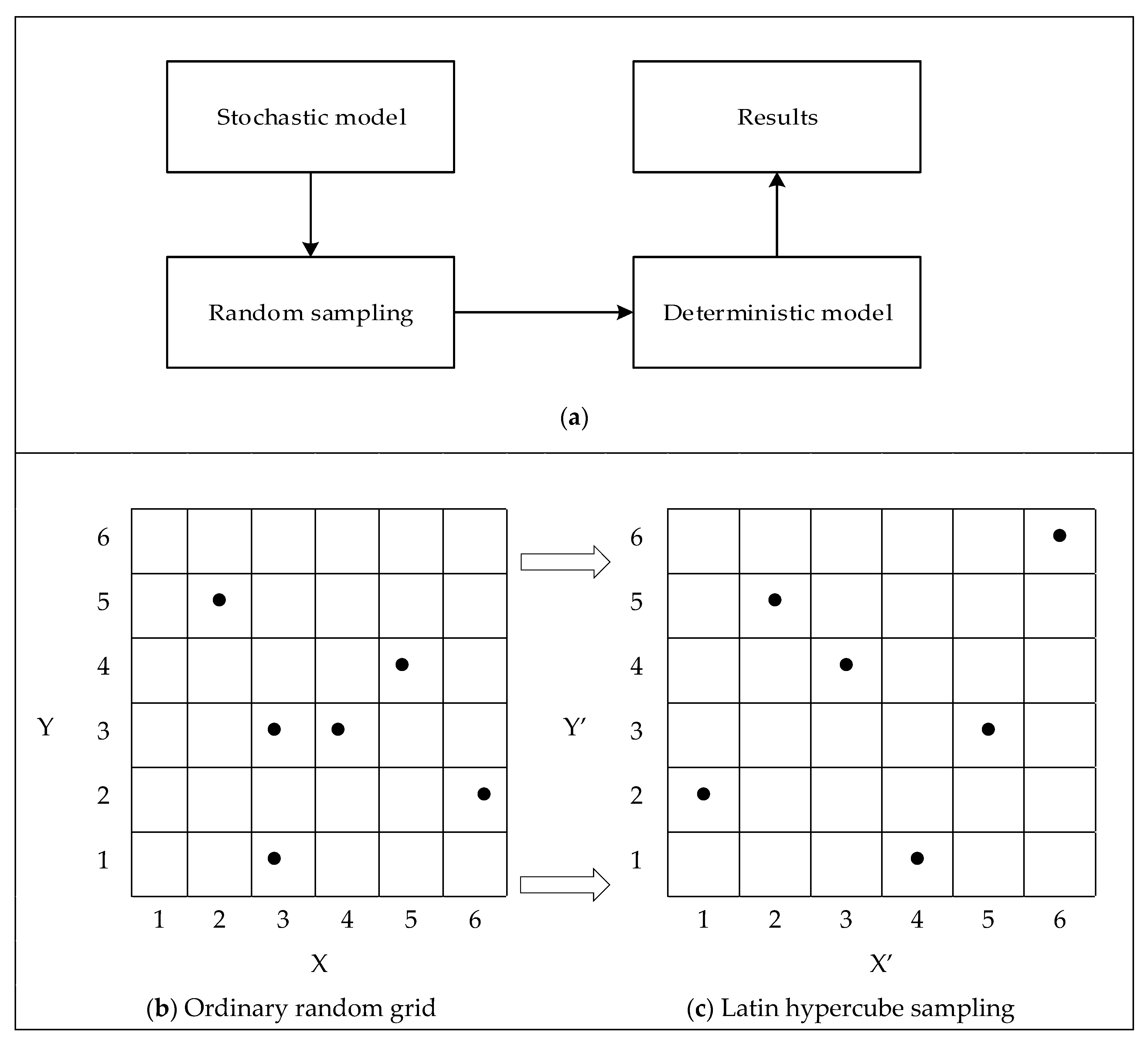
In uncertainty quantification, the Monte Carlo system uses mixed model statistics to obtain the results of a random system. The Monte Carlo strategy entails a GridMatch tool comprising three stages. The three phases, which include the stochastic model, random sampling and deterministic model, are the components of the optimisation approach used in the analogous implementation of the TeDP of the Monte Carlo method. To obtain samples of random parameters, an individual can use a pseudorandom number generator. The generator tends to construct a sequence of numbers in a deterministic fashion, in which it indexes the numbers based on the value of a seed. The seed emulates a cluster of random numbers. If any two categories of responsibilities have common varieties of seeds, they can generate a conventional system of random numbers. To avoid the production of conventional seeds, it is imperative to employ a vital seed scattering tactic for all the electrical components. The appropriate approach can create a seed for each electric bus, without replication. The tactic must also warrant exclusive categorisation of the numbers from each electric bus. Figure 5 in section (a) represents an overview of the Monte Carlo algorithm while part (b) and (c) demonstrate the random sampling filtration process using a stochastic model as Latin hypercube that is explained in Section 5.2.

5.1.1. NASA N3-X Case Study

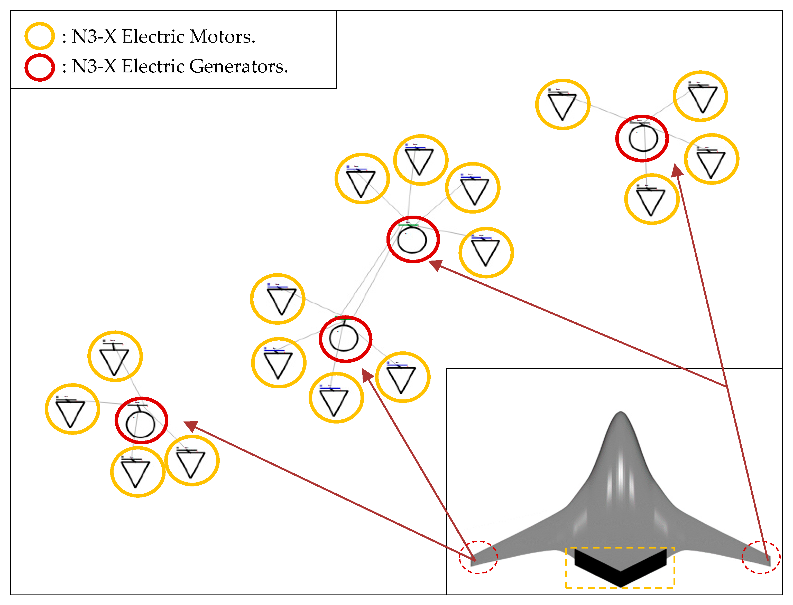
The case study used for TeDP uncertainty and error estimation is NASA N3-X. The aircraft is modelled with 16 motors and four generators with different data inputs, depending on the system situation. Three types of aircraft condition assist in the uncertainty and error estimation to test the reliability of each state. The three examined conditions are rolling to take off (RTO), taking off (TO), and cruising. Quantitative risk analysis was conducted using Cranfield University’s in-house software extension for “TurboMatch,” called “GridMatch.” The assumptions were used in Monte Carlo 3 precision for a maximum of 1000 iterations. Figure 6 represents the system model on GridMatch for NASA N3-X to measure the electrical grid performance.

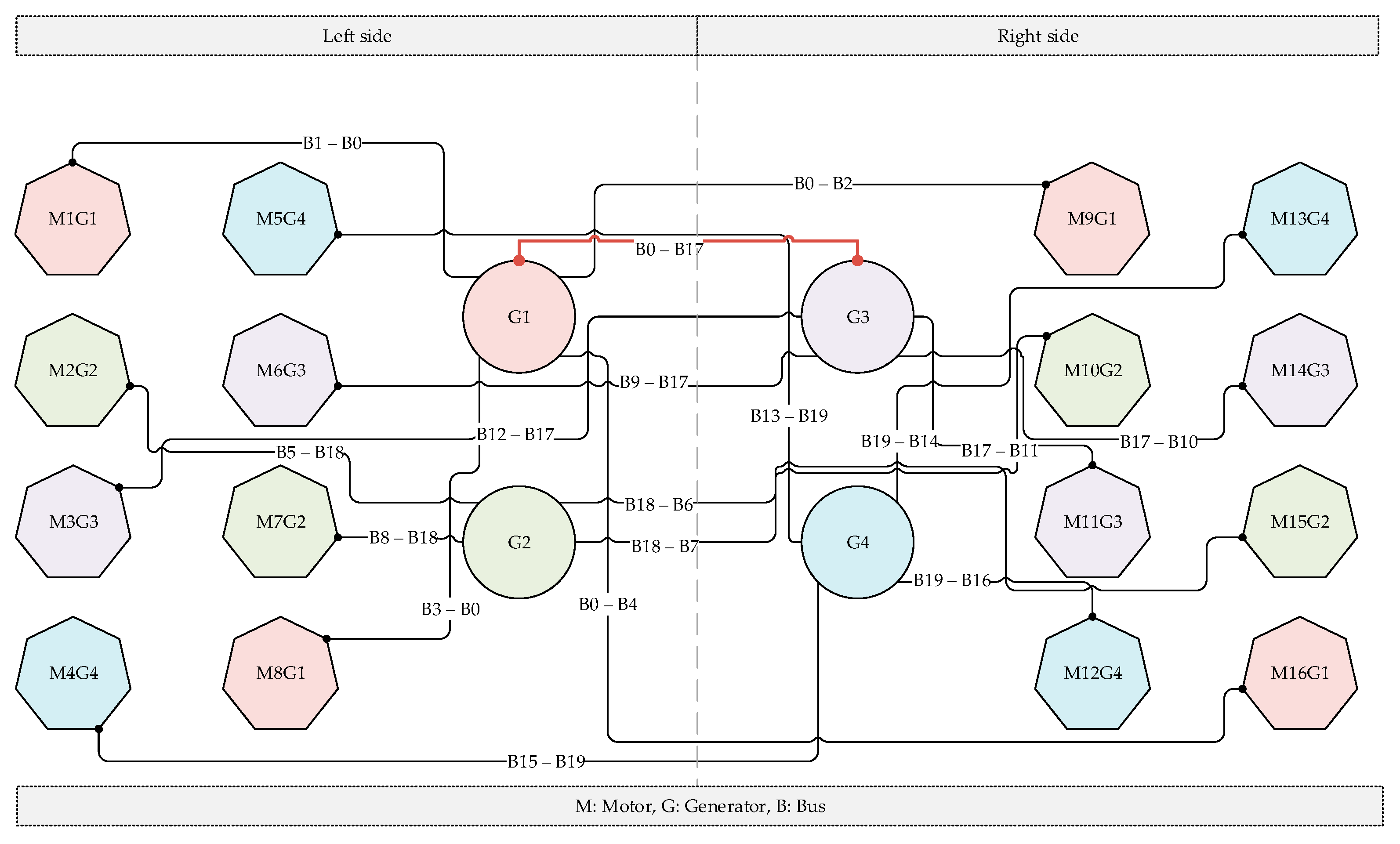
In this state of NASA N3-X, the modelled power for each motor is calculated to be 3.588 MVA, and that of each generator is 14.352 MVA [24]. There is a connection between generators 1 and 3, as a risk redundancy plane, which is the same for generators 2 and 4. Moreover, the 16 motors are connected in a mixed prime generator, and every fourth motor is aggregately connected to one generator. Figure 7 illustrates that NASA N3-X model used.

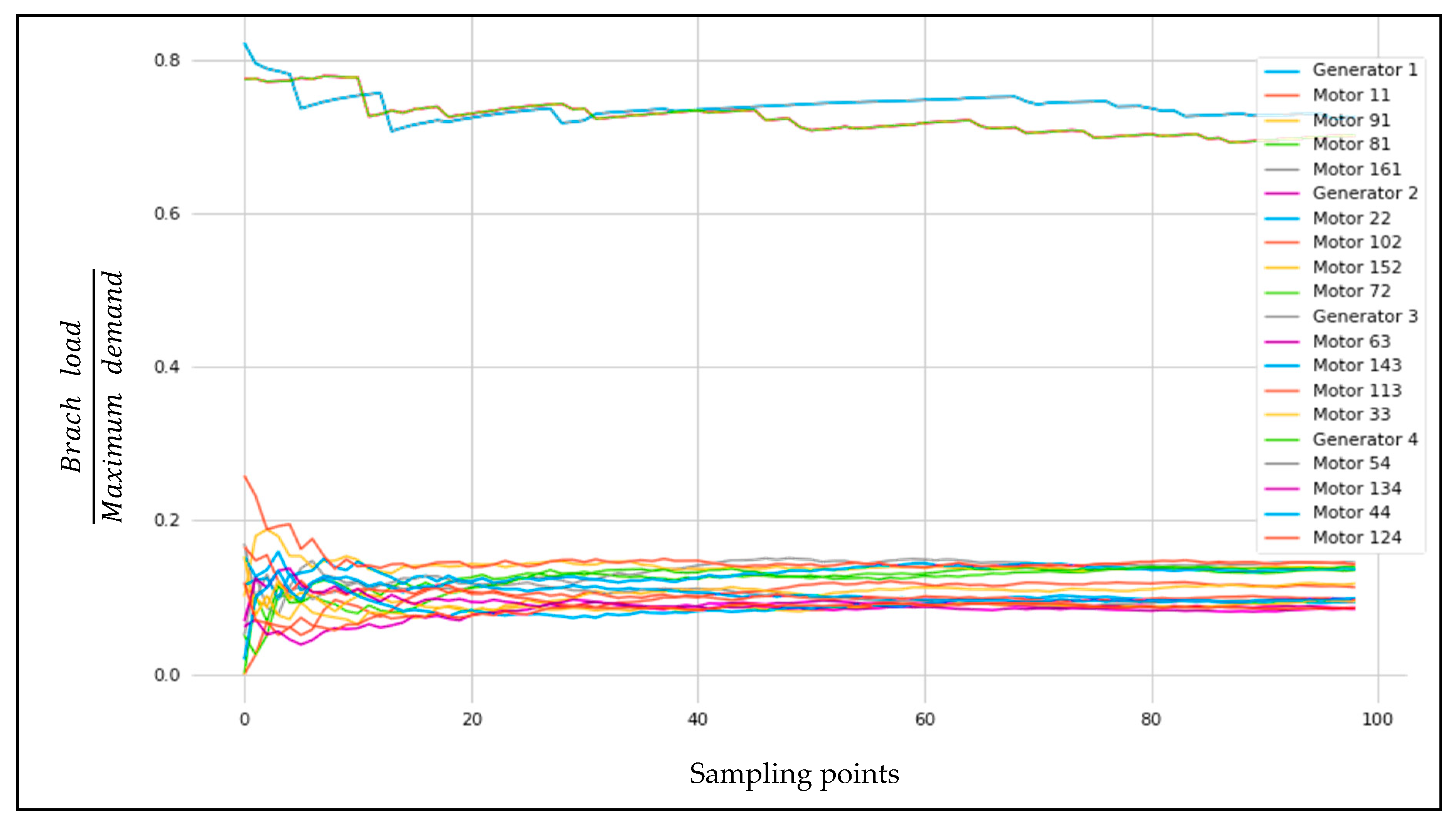
5.1.2. Rolling to Take Off (RTO)

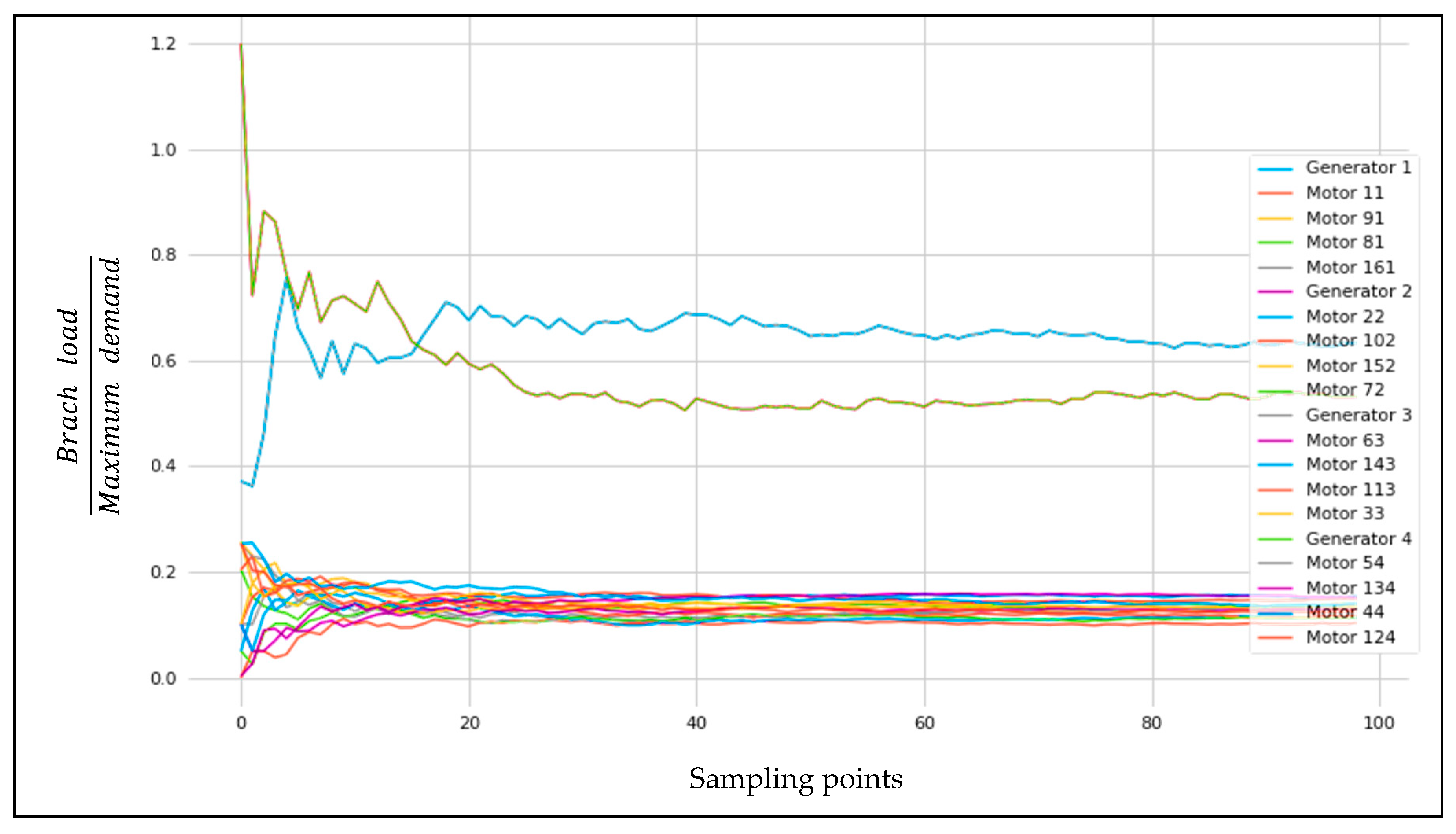
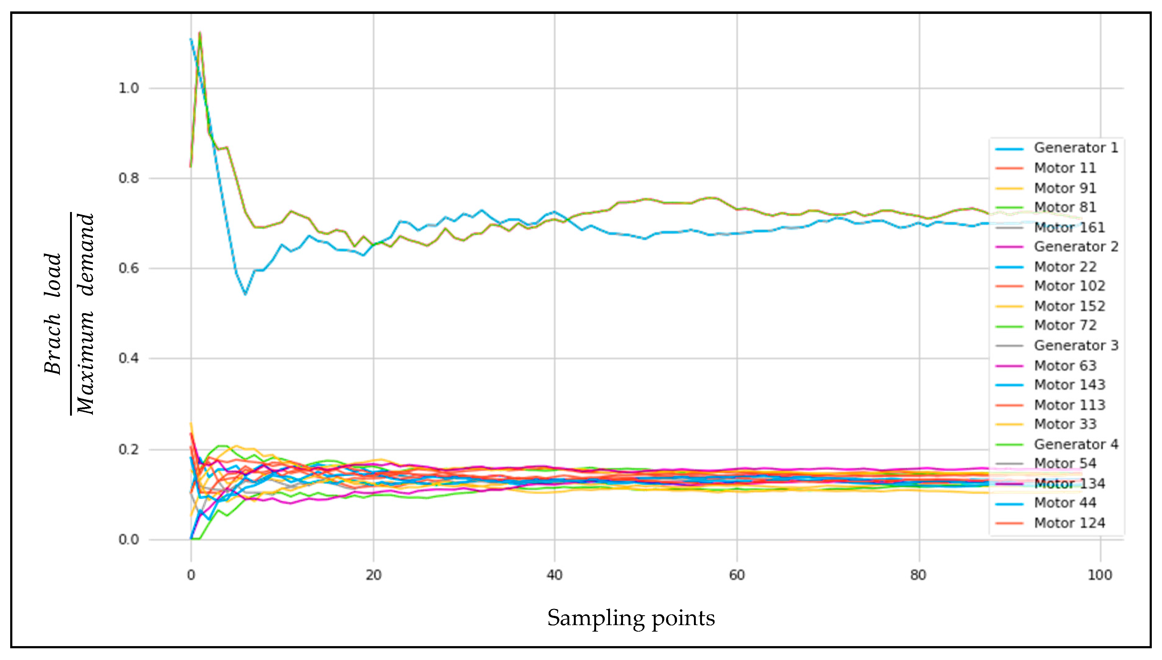
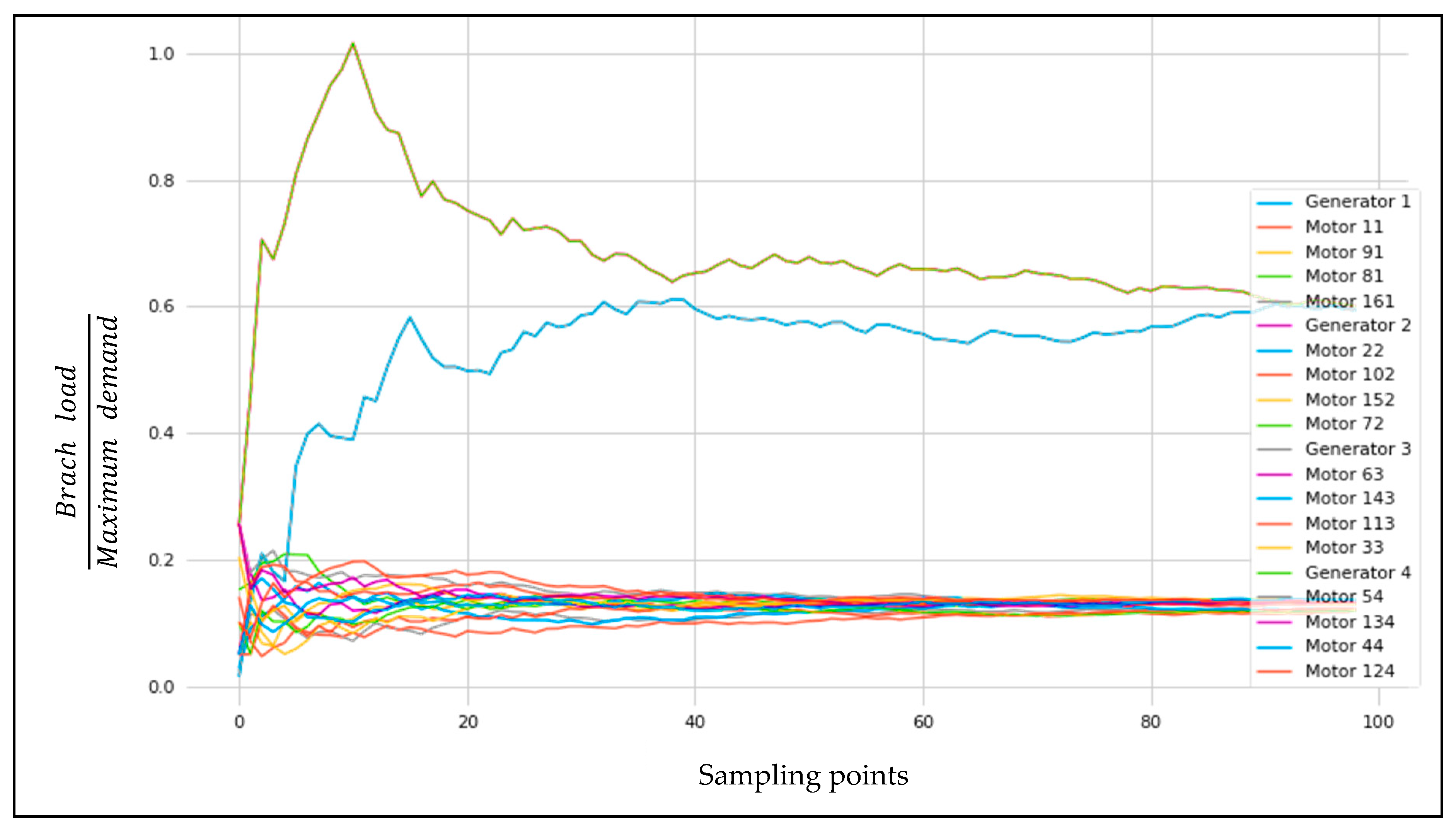
Figure 8 illustrates the risk analysis result of NASA N3-X for the branch loading average. The results show how confident the probabilistic power flow of the modelled system is. It indicates from the x-axis that the first 20 samples have a higher probability of overload, and then there is a stabilisation in confidence. While all samples ran in the same numerical simulation, the results divertive in the first samples as the sampling method build upon initial results. This means that the error in the first result is reducing until the saturating outcomes. The average confidence probability results for the primary and secondly generators are 70% and 50%, respectively, where the motors are from 15–17%. This means that the system is reliable for the RTO condition in terms of the load, as the calculated determined load need for motors is 68%, and this is covered by 70% of the Monte Carlo consequence.

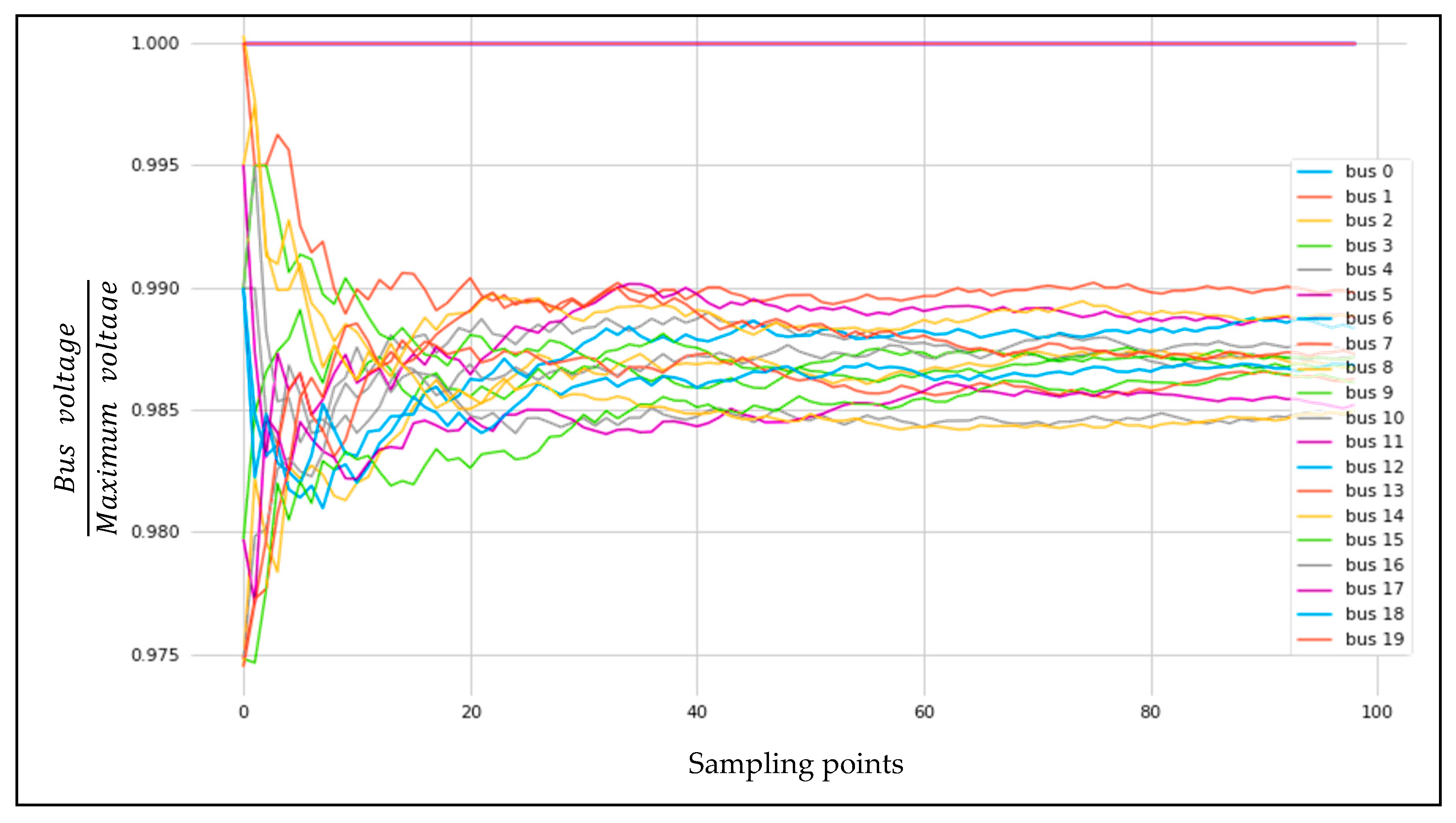
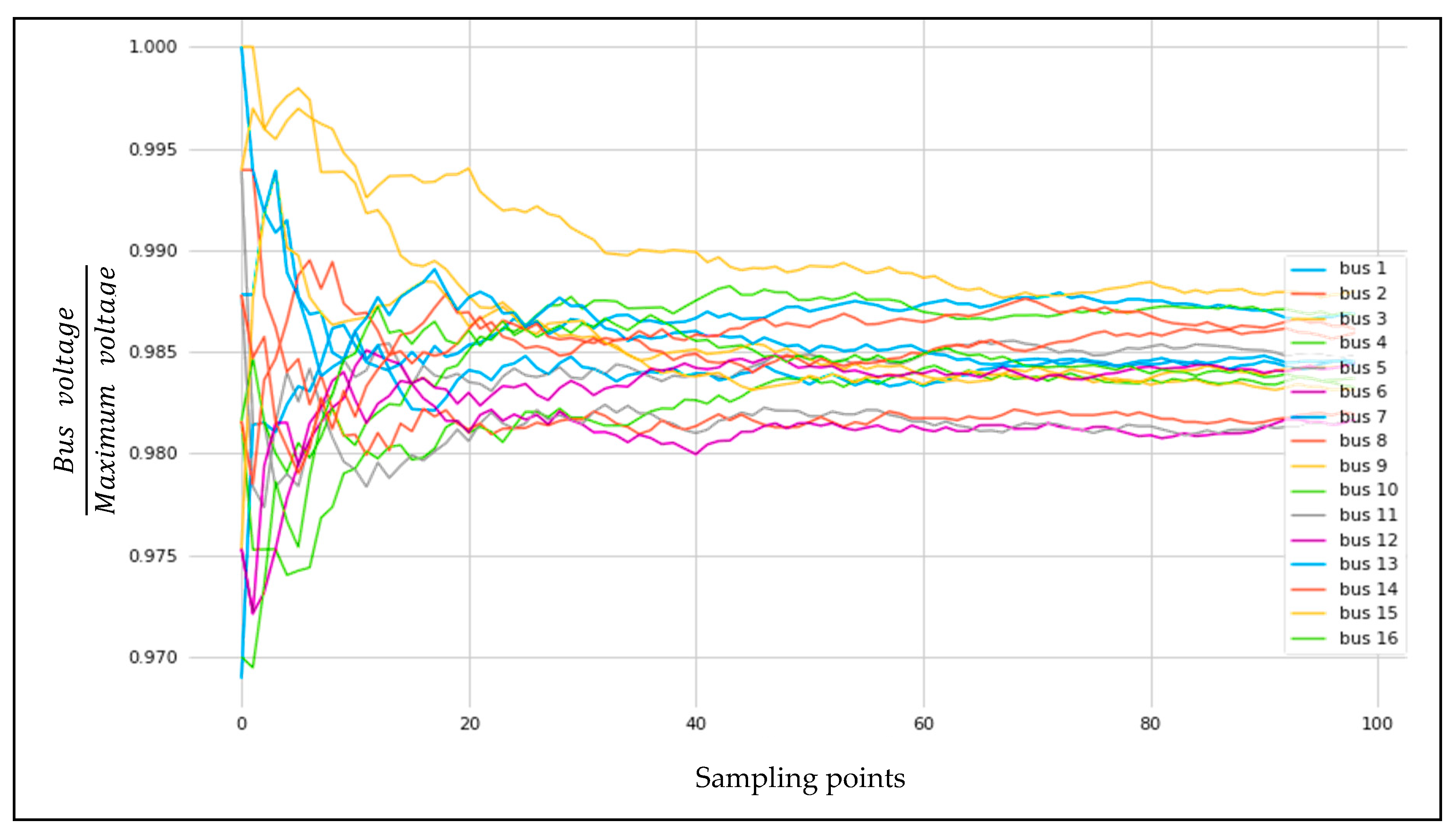
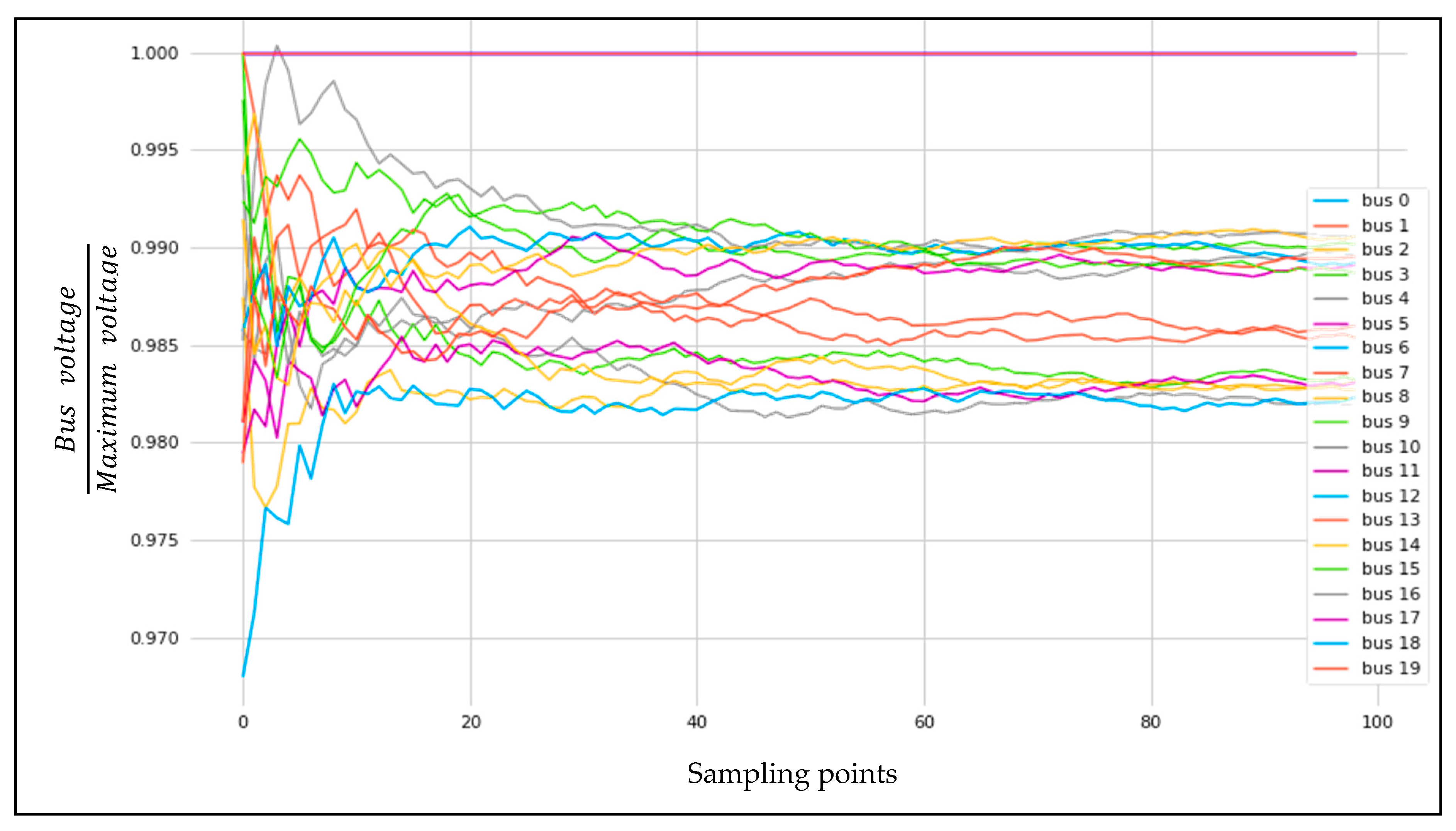
Figure 9 shows the NASA N3-X bus voltage average from the Monte Carlo analysis. Appositive outcomes are given from the analysis, with a fixed voltage, through the electric bus from the power supply generators to the motors. The confidence percentage of the motor bus is from 98.4% to 99%, based on the bus condition. From these analyses, the bus loss was found to be within 0.6%–1% of the total electric grid resonance of the inductance of the magnetic field and produced heat.

5.1.3. Taking Off (TO)

This assessment scenario represents a supreme load of energy and, as in taking off (TO), the full thrust is needed to drag the aircraft. The same assessment and tools in RTO are used in TO, except the input power calculated for the motors, which is 4.282 MVA and 17.129 MVA for each generator. In Figure 10, the results confirm that the load for both generators average 70%–78%, while those for the motors remain the same as for TO. Additionally, in Figure 11, the confidence of the voltage average through the bus is reduced from 98.7 to 98.1 in terms of the fixed power voltage from the generator source. This means that the inductance and heat resistance increased under this risk assessment condition.

5.1.4. Cruising

This situation was considered as the lowest in terms of power consumption and confidence in precision. In the cruising condition, the generators were calculated to be 5.237 MVA, and the motors were calculated to be 1.309 MVA, with the same assumptions for RTO and TO. The average confidence possibility for the branch reliability of the power is 68% for primary generators and 81% for the secondary generators. However, the reliability of the motor remains the same for the motors, as in RTO and TO, as shown in Figure 12. For the voltage bus risk assessment, the outcomes, as presented in Figure 13, illustrate projected certainty levels of 98.1%–98.7%.

5.2. Latin Hypercube

The Latin hypercube algorithm involves a stratified sampling methodology that applies to several variables. It mainly serves as a technique through which users can reduce the number of runs necessary for a Monte Carlo simulation to enhance the accuracy of the random distribution [25]. It is possible to integrate a Latin hypercube sampling technique into a Monte Carlo model and operate it with the variables involved based on any analytical probability distribution. As for the uncertainty quantification and error estimation, risk optimisers can distribute the cumulative curve into equivalent intervals, based on the cumulative probability scale [26,27]. The subdivision can enable the risk optimiser to pick a random value from every interval of the input distribution. It is evident that, with Latin hypercube sampling, risk optimisers can work with a predetermined number of values because the number of intervals achieved must be equivalent or correspond to the number of available iterations. It is essential to understand that there are no longer pure random samples. As a result, the central limit theorem of statistics is not applicable [28]. Latin hypercube sampling, however, entails stratified random samples. In uncertainty, consistent monitoring of the process can be achieved from the beginning to the end regarding the quantification and error estimation processes in turboelectric numerical risk modelling optimisation. Ideally, it can constrain the information for every simulation to ensure that it can correspond very closely to the input distribution. The uniformity of all iterations becomes achievable across the simulation. It is crucial to understand, however, that, although it is possible to constrain the data for the iterations of a simulation to correspond to the input distribution as a cluster, it is impossible to achieve that for any particular subsequent iteration.

The benefit of the Latin hypercube technique is that, even for the modest amounts of iterations, the Latin hypercube technique can converge all the sample means, allowing them to fall into a small segment of the standard error. It should be recalled that the objective of Latin hypercube sampling is to spread the sample points uniformly across all the possible values. As a result, during the uncertainty quantification and error estimation processes, the Latin hypercube sampling method can enable a wide range of parameters involved in the turboelectric numerical modelling process to be considered. Therefore, it can incorporate these parameters into the uncertainty quantification and error estimation procedures. As a result, it can generate common and reliable mean values, from which relevant and accurate predictions can be made. Latin hypercube sampling is flexible because, although it generates a sample from each interval in an iteration and ensures that there is no correlation between different inputs, it can also enable determination of the correlation [29]. In other words, the Latin hypercube algorithm is a method mechanism for sorted random iterations of multidimensional distribution values. The algorithm of this method starts with median Latin hypercube sampling, integrating the median value of every equiprobable interval, and then random Latin hypercube sampling picks a random point within an interval. The following

Table 1. Monte Carlo and Latin hypercube comparison.

Monte Carlo	Latin Hypercube
More samples for better performance	Fewer samples for better performance
Memoryless	Memory
Increases computational complexity	Decreases computational complexity

shows the comparison between Monte Carlo and Latin Hypercube.

5.2.1. NASA N3-X Case Study

The Latin hypercube method, used for NASA N3-X in 100 sampling points, results in realistic outcomes. The same three scenarios—RTO, TO, and cruising—are subject to quantitative risk analysis using a similar tool. The purpose of this assessment of pure randomness is to associate the Monte Carlo outcomes.

5.2.2. Rolling to Take Off (RTO)

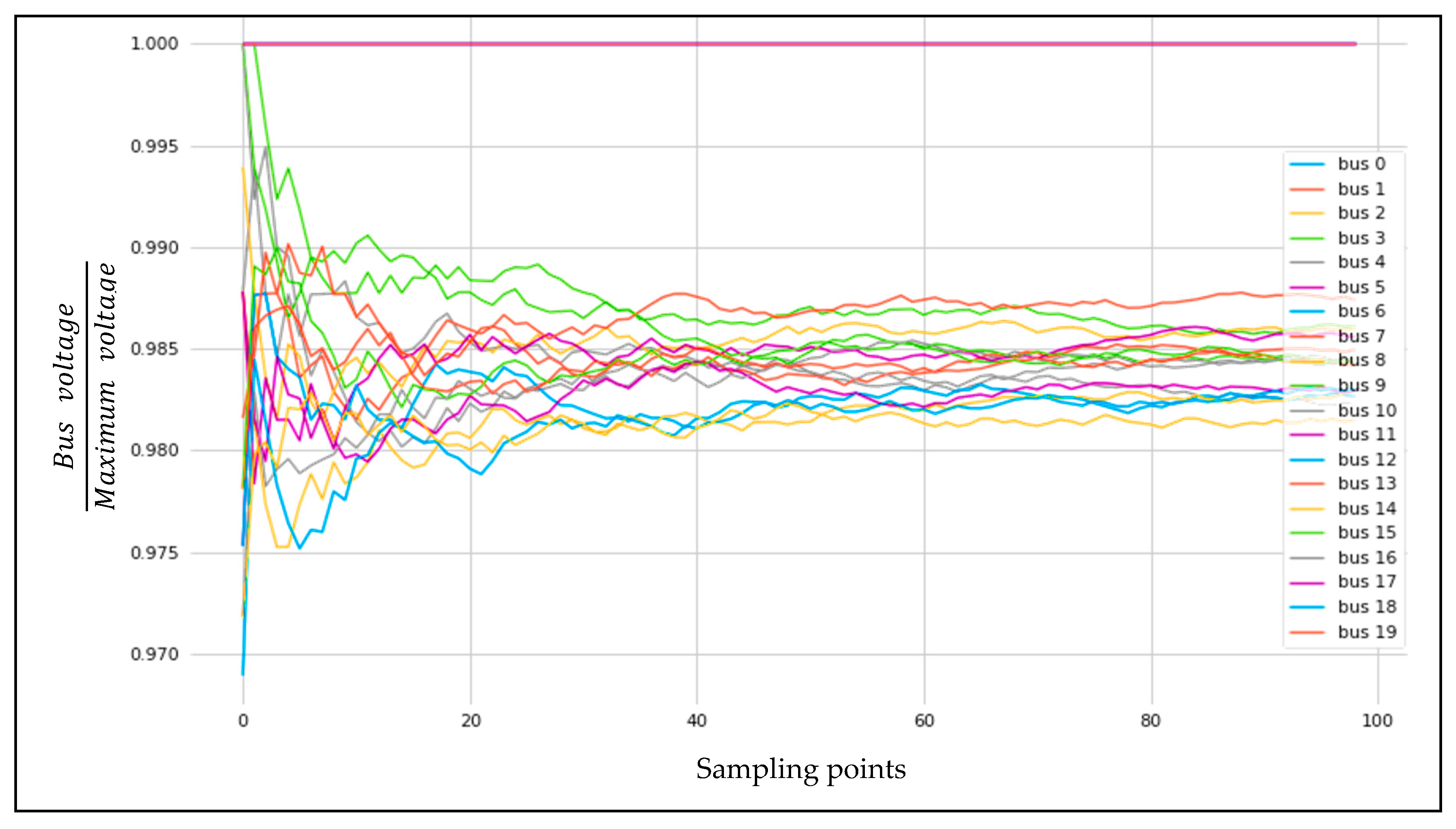
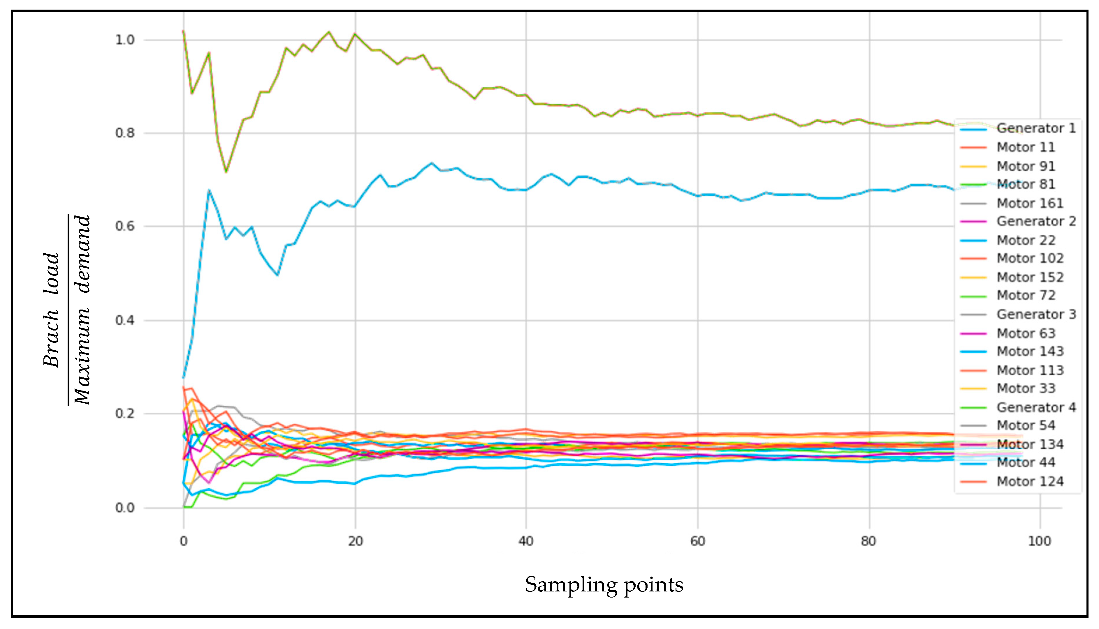
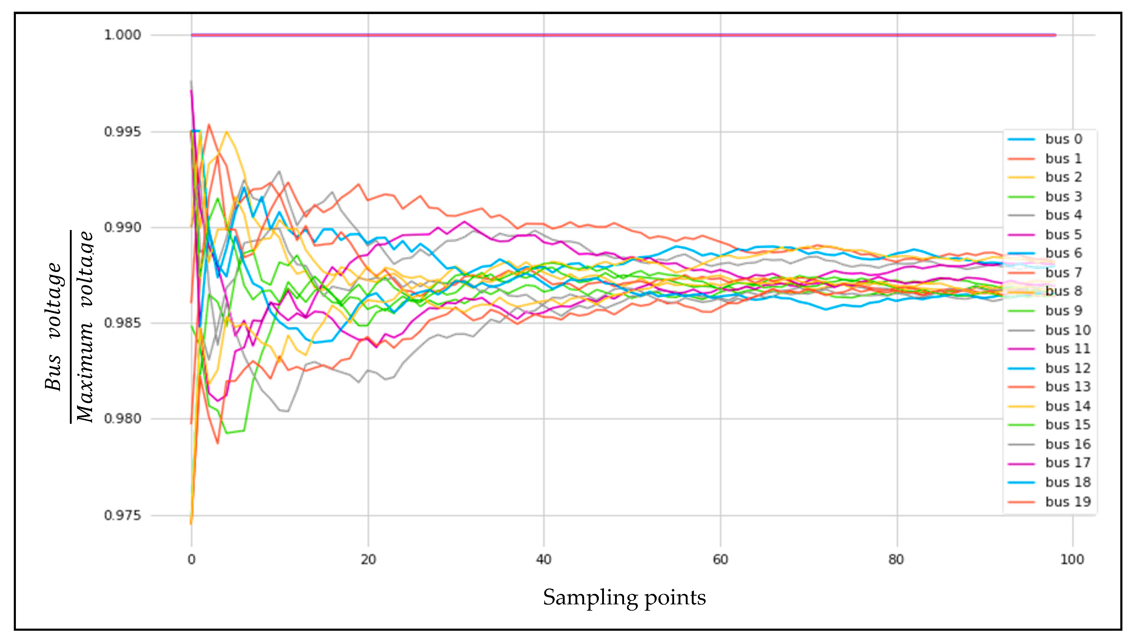
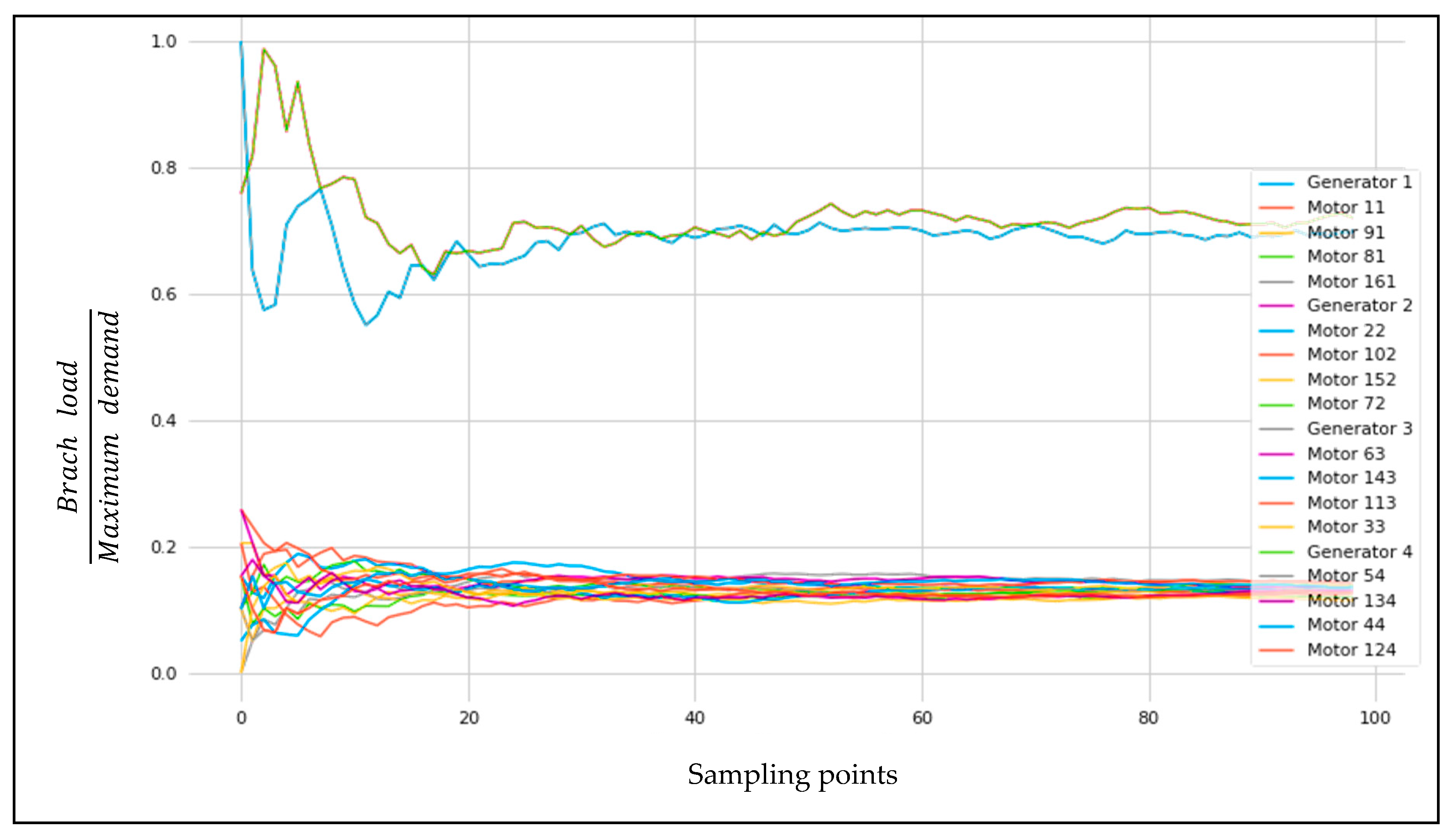
With similar inputs as those in RTO in Monte Carlo, the Latin hypercube simulation provides more accurate results after 38 sampling points, and the system shows a 60% average load power for primary generators and 63% for secondary generators. The equivalent accuracy for the motors at the same sampling points is 15%–16% of the confidence percentage, as shown in Figure 14. The voltage stability in this method of analysis in RTO shows 98.6% to 99% for the motor buses, with the assumption of a fixed power source. Figure 15 illustrates the outcome of the Latin hypercube for each bus in the electrical model grid for NASA N3-X under the RTO condition.

5.2.3. Taking Off (TO)

The result in this stage, with the same inputs used in TO in Monte Carlo, shows that the stability load of the generators has a lower number of sampling points than RTO in the 18 samples, and the primary and secondary generators fluctuate between 70% and 73% of the power load. However, the motors are 1% higher than those in TO using the same analysis method, and the load percentage is within 16%–17%, as presented in Figure 16. In the bus analysis, the confidence reliability is 0.3 to 0.7, in 98% of the motors, as shown in Figure 17.

5.2.4. Cruising

The last station to test with the Latin hypercube is the cruising state. The inputs, as in Monte Carlo, show that the confidence reliability for both the primary and secondary generators range from 71% to 76%. In addition, the motors are considered to be within 14%–17% of the branch load, as shown in Figure 18. Figure 19 shows the bus voltage average to be between 98.3% and 99.3% of the probability confidence.

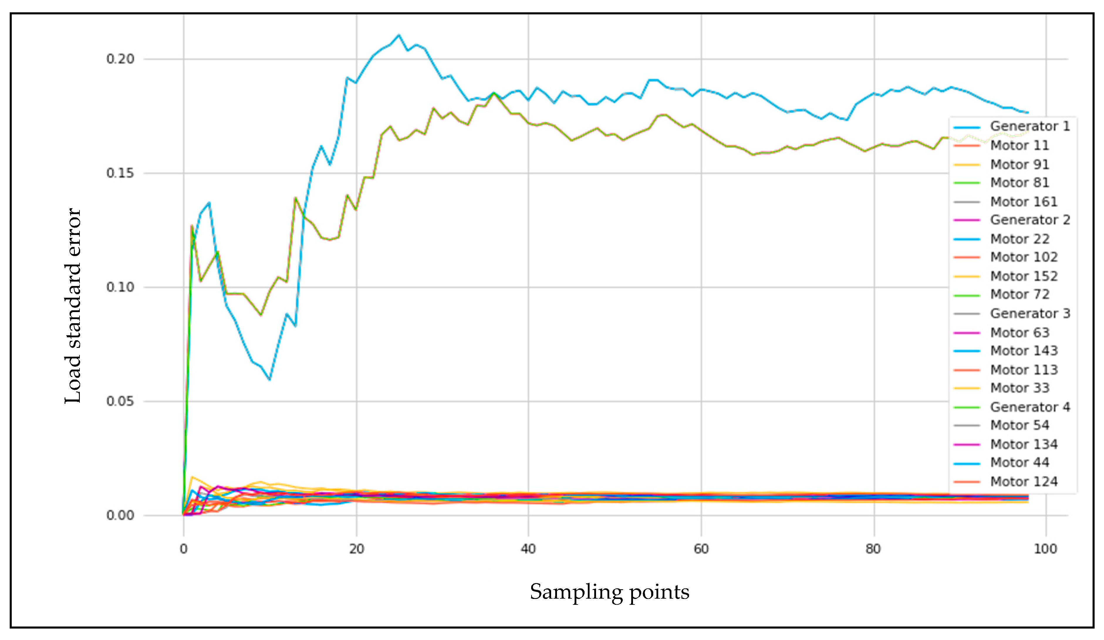
6. Standard Deviation

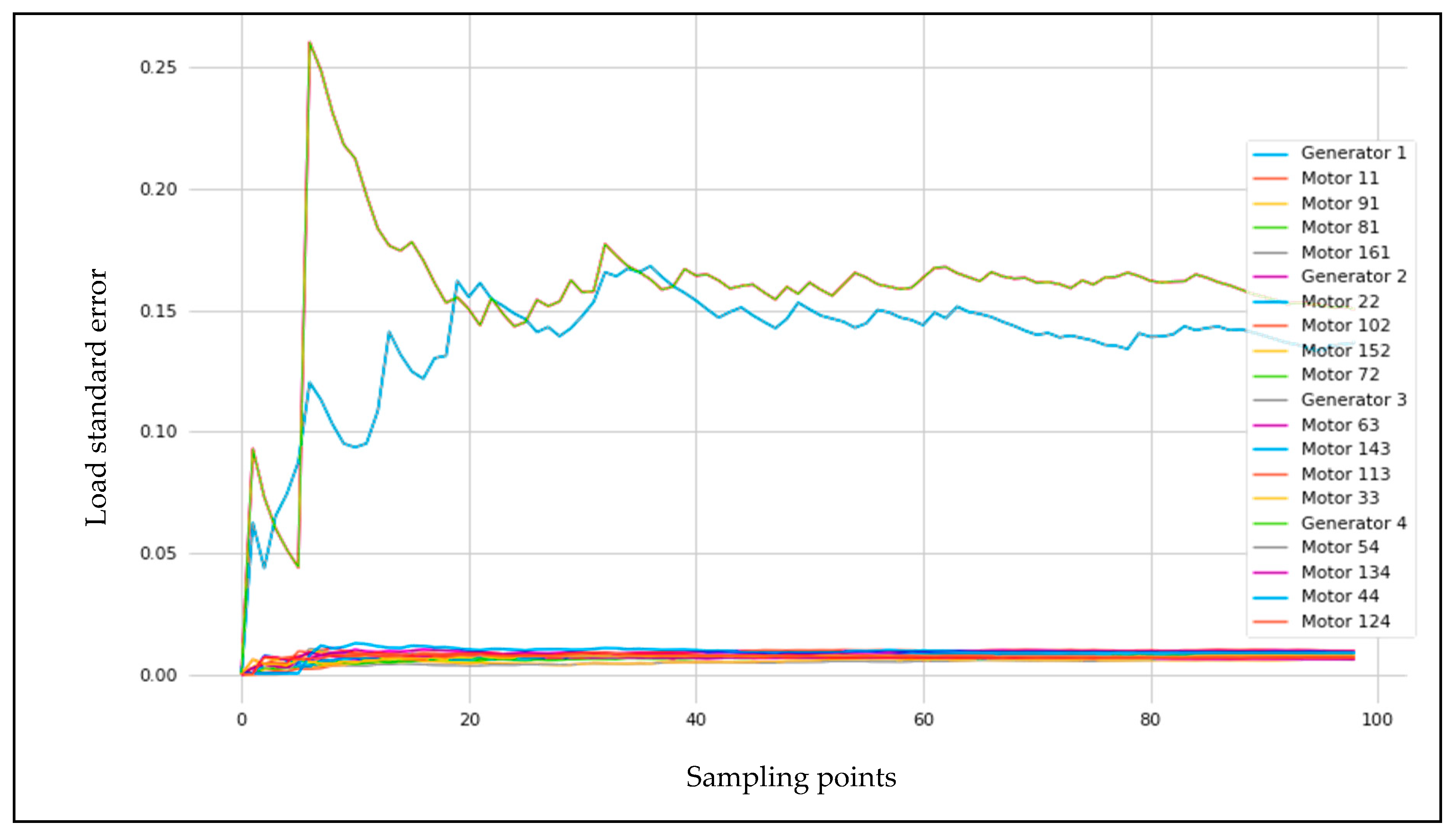
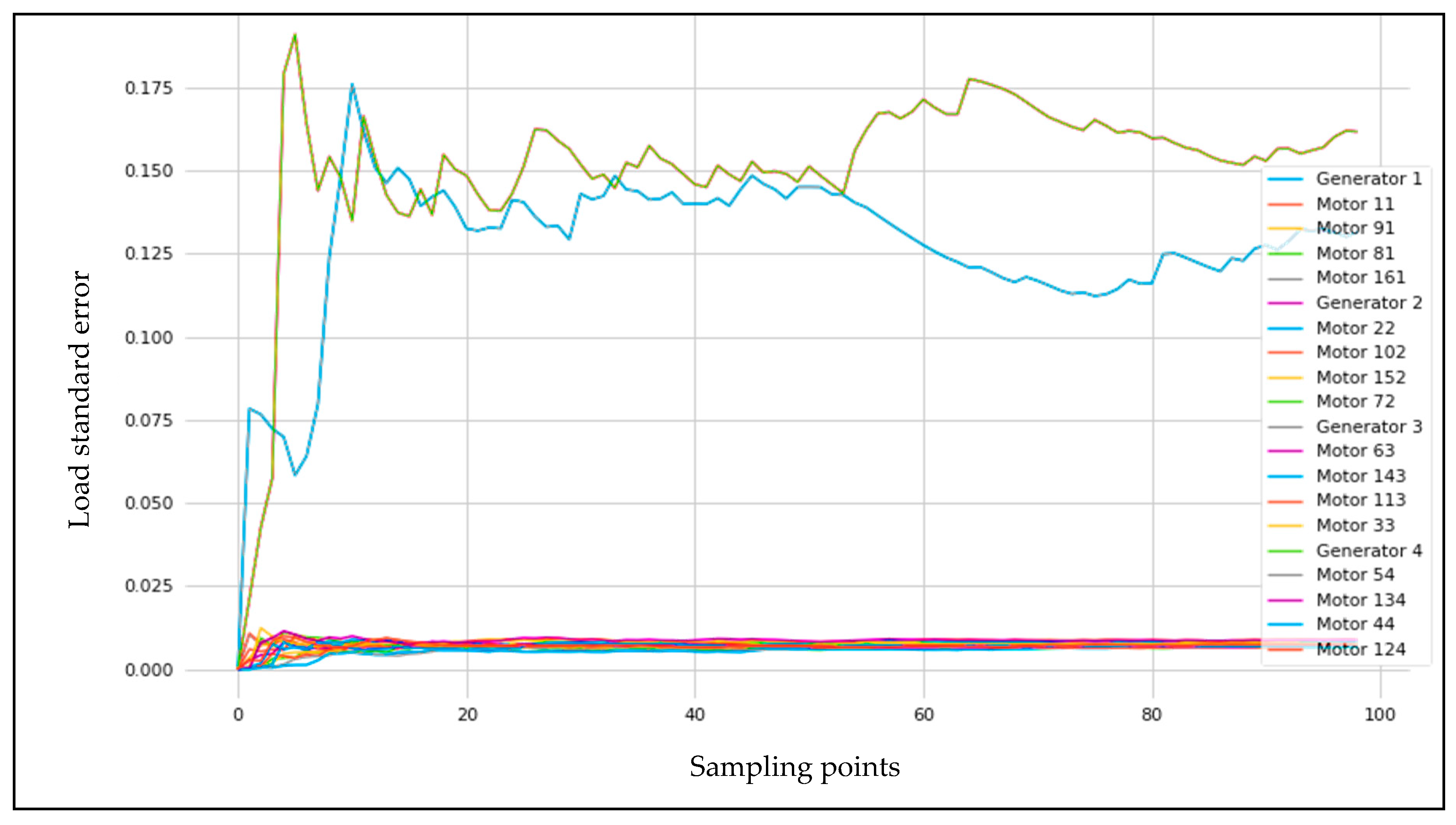
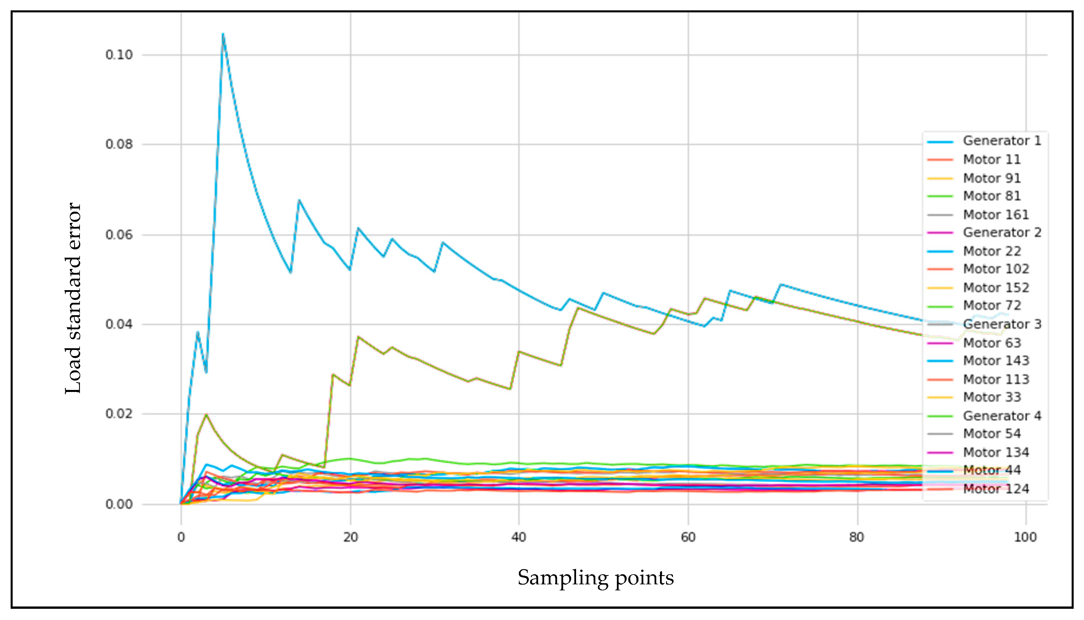
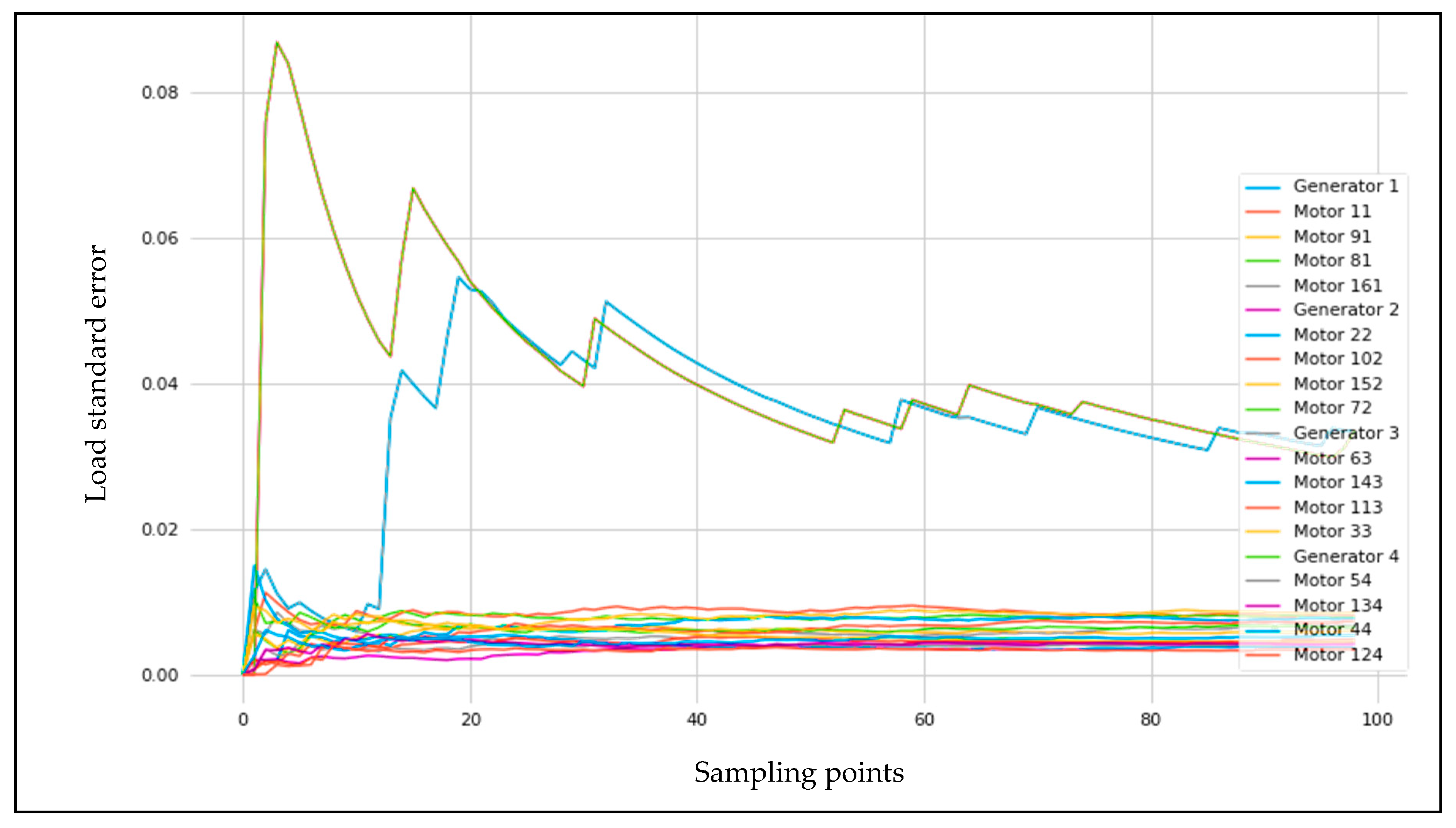
As a significant number of sampling points are used in the Monte Carlo (MC) and Latin hypercube (LH) methods, error limitation is performed using the standard deviation for branch loading as a variable. The error estimation defines the maximum level of specific output accuracy from the applied numerical model. It was applied in all flying conditions and for both analysis methods. The following results can be observed:

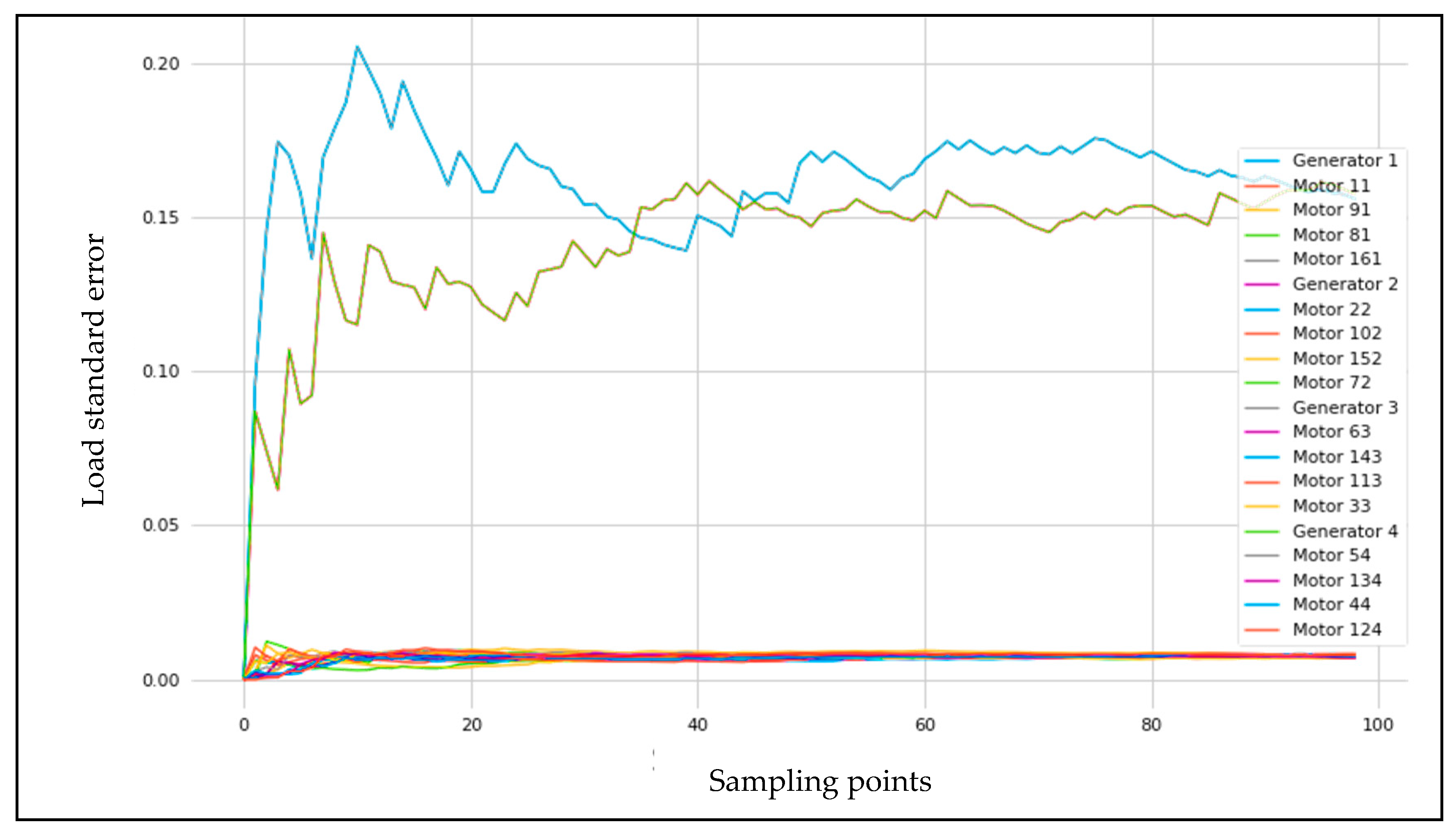
• RTO: This stage shows an error estimation for MC analysis of less than 0.01% for the motor branches and 0.17% and 0.16% for the primary and secondary generators, respectively, as shown in Figure 20. On the other hand, the error eviction of LH was less than that of MC with the same inputs and case studies, as shown in Figure 21.
• TO: This stage shows an error limitation of less than 0.01% for the motor branches and 0.14%–0.16% for the generators as an outcome of the MC method. Figure 22 and Figure 23 illustrate the MC and LH standard deviations for the TO case study.
• Cruising: In this stage, MC and LH have practically matching results in terms of the error margins, and Figure 24 and Figure 25 show these data.

7. Cumulative Distribution Function

This probability density function, called the cumulative distribution function (CDF), is the probability that the function of a variable will take less than or equal to r, and all variable submissions are equal to 1. It can be expressed as follows:

$$f\left(x\right)=P\left(X\le r\right)$$

where X = added variables; r = random variables.

CDF is a statistical method used to eliminate the probability limits between 0 and 1 to study the branch load level on the electrical grid [30]. This analysis includes MC and LH results with the three scenarios, RTO, TO and cruising. The following

Table 2. Standard deviation and cumulative distribution function comparison.

Standard Deviation	Cumulative Distribution Function
Error sizing	Represents the sampling from 0 to 1
Data convergent margining	Examines the data distribution

shows the comparison between Standard deviation and cumulative distribution function.

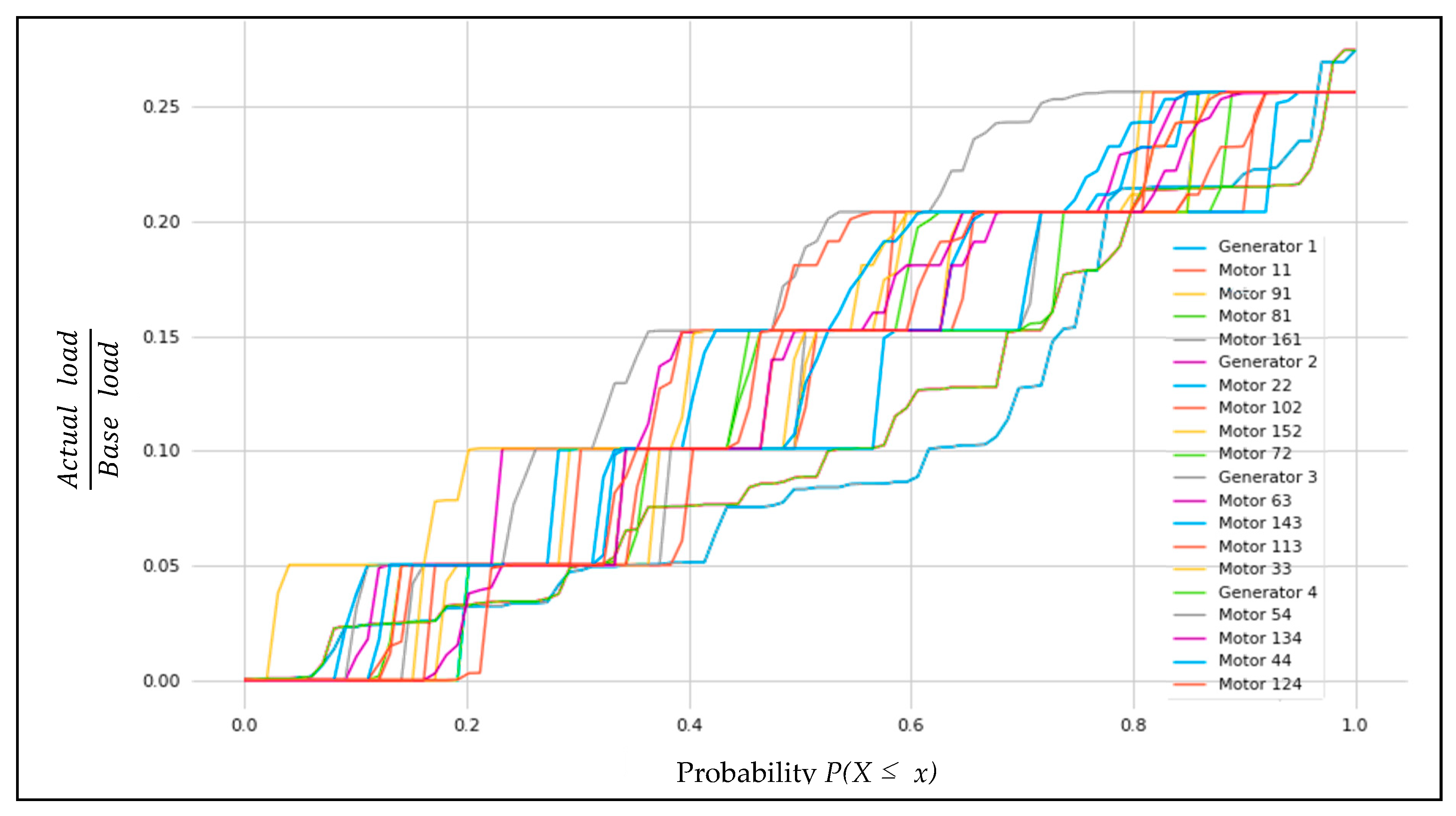
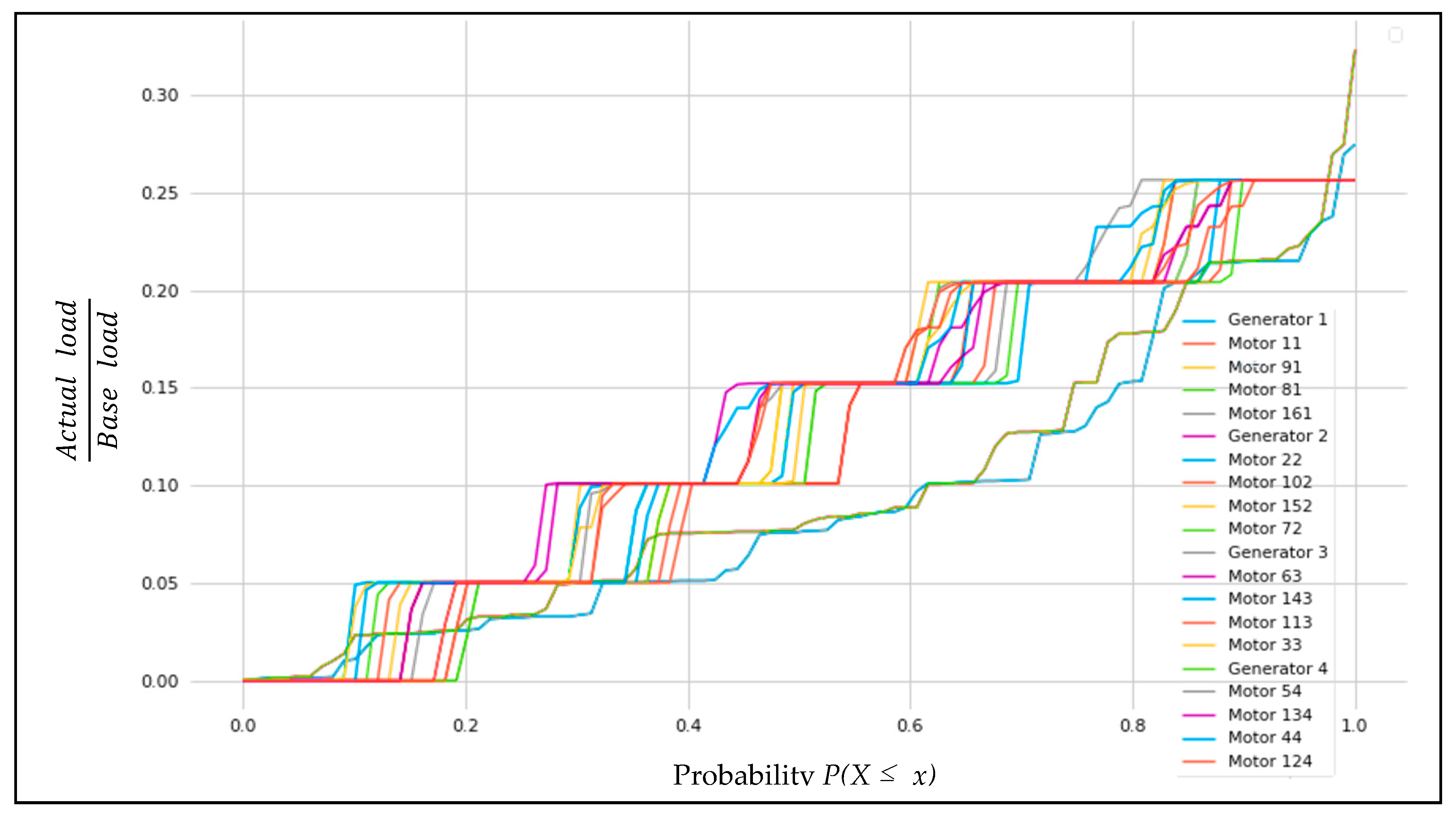
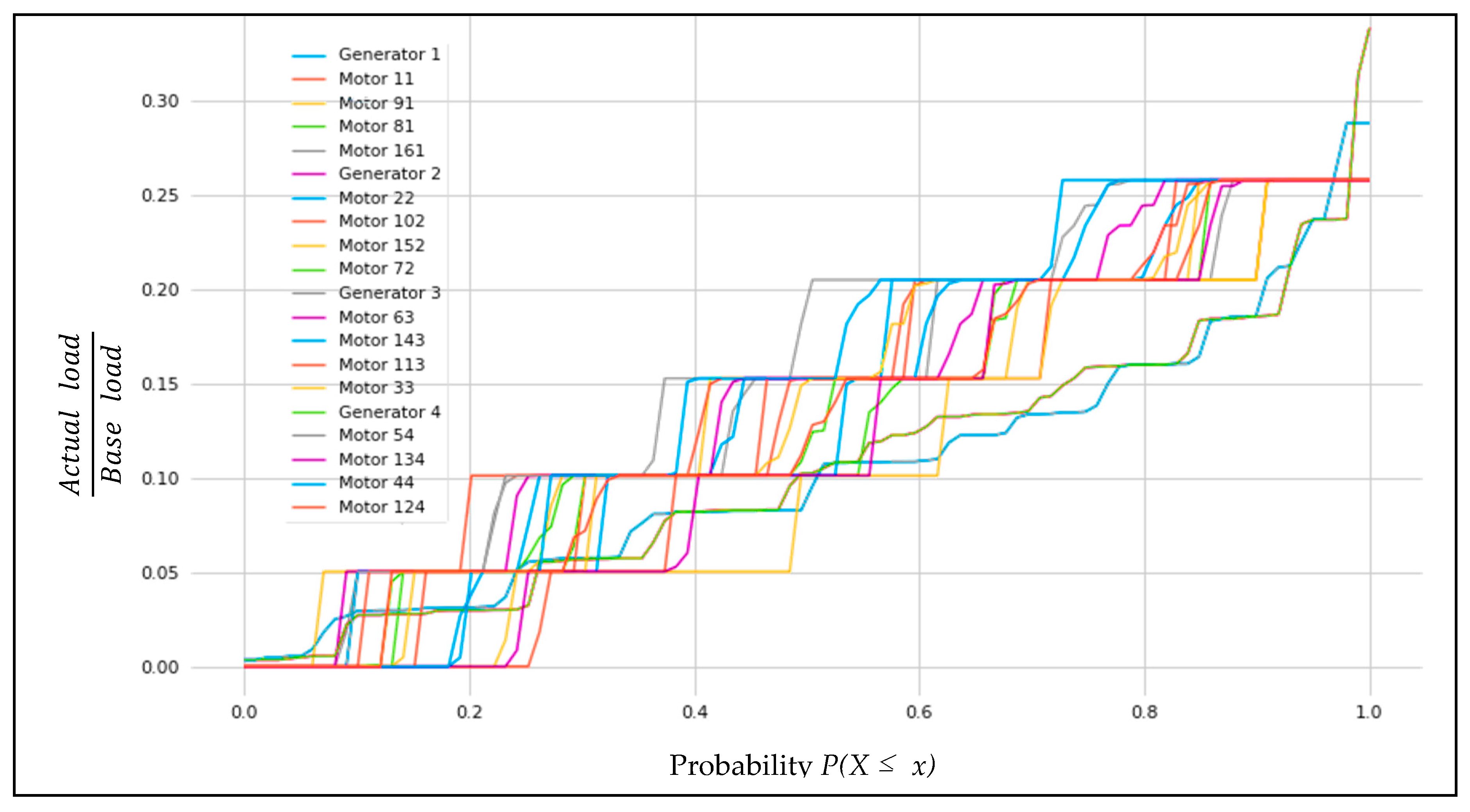
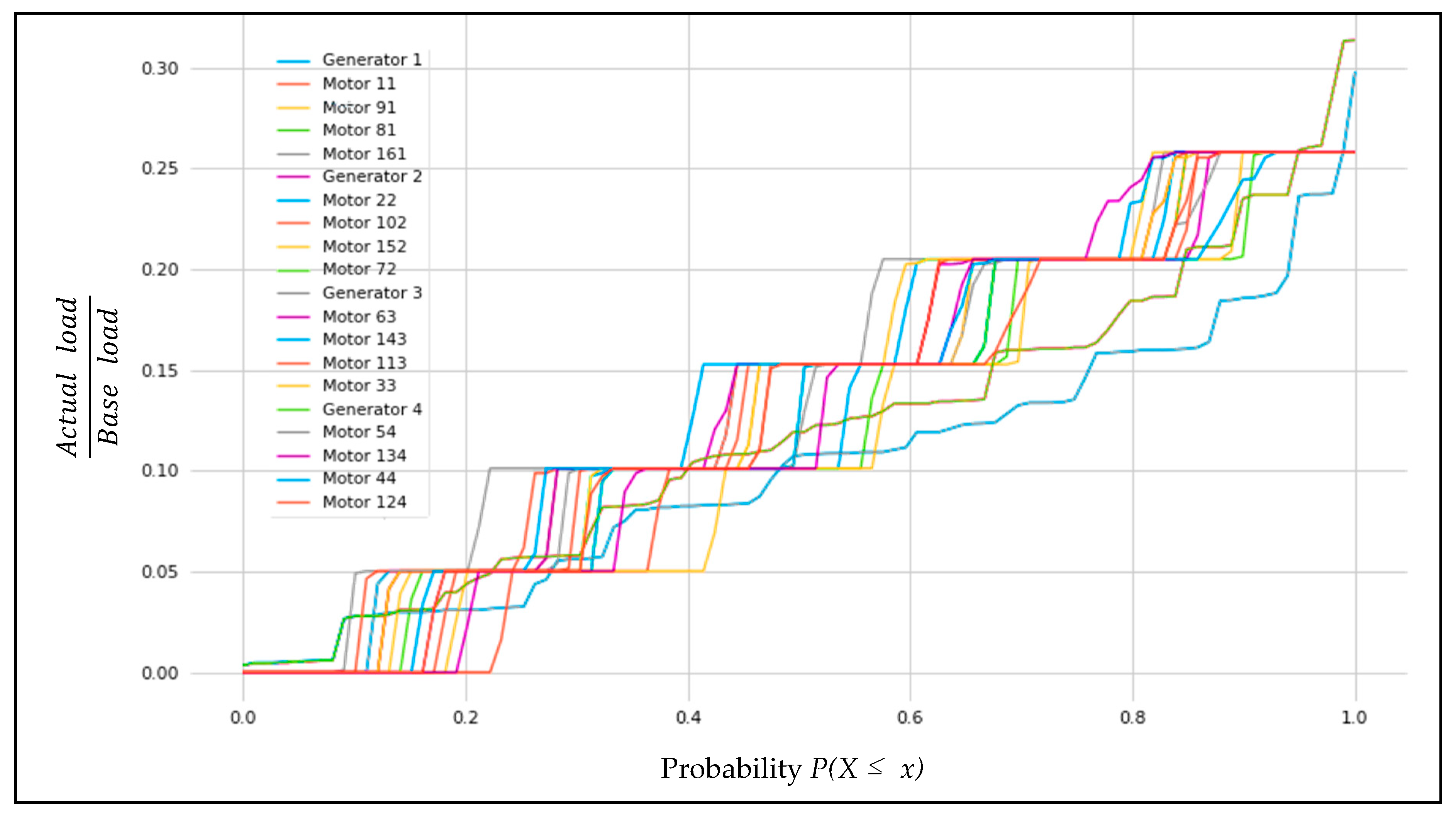
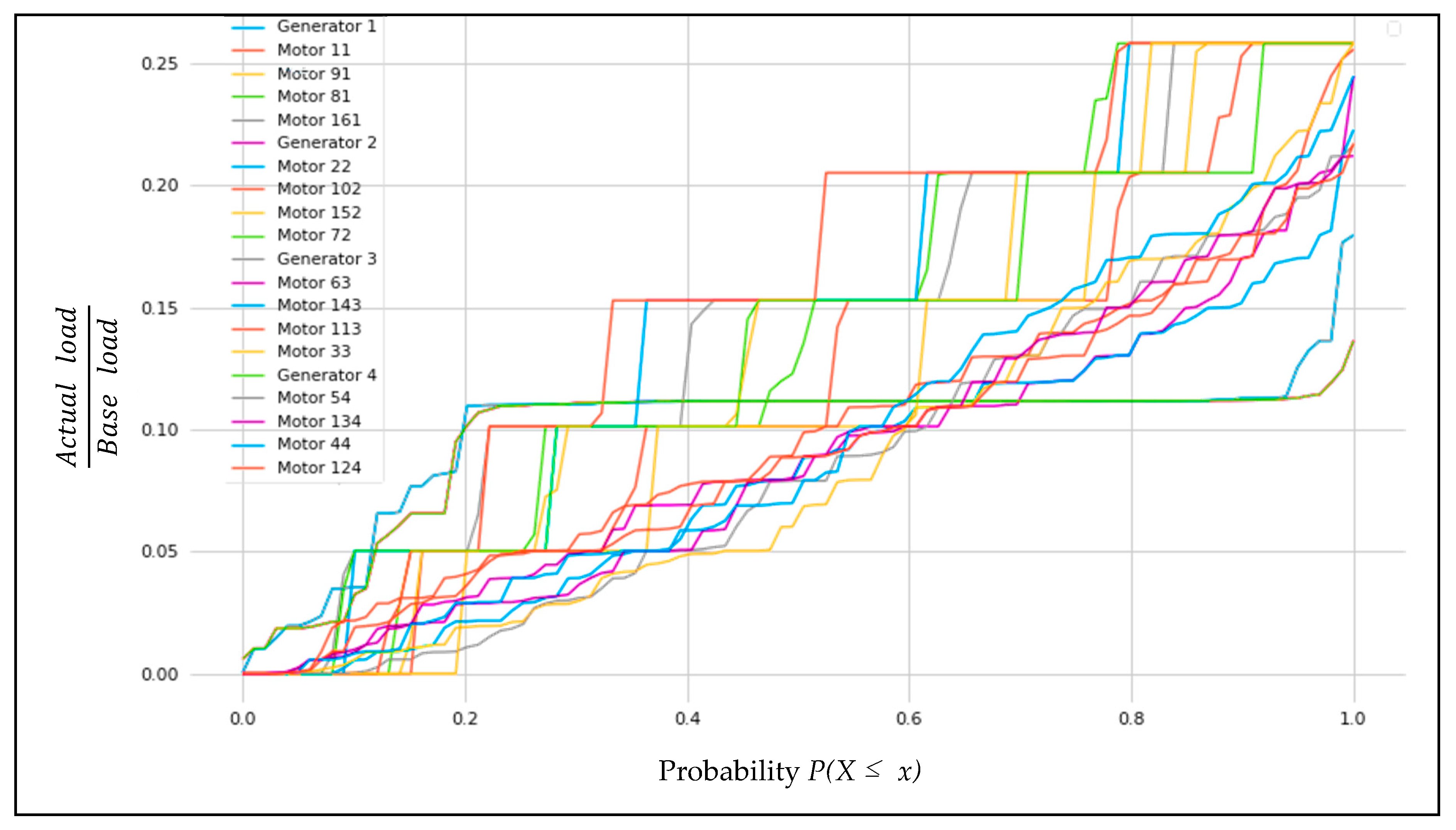
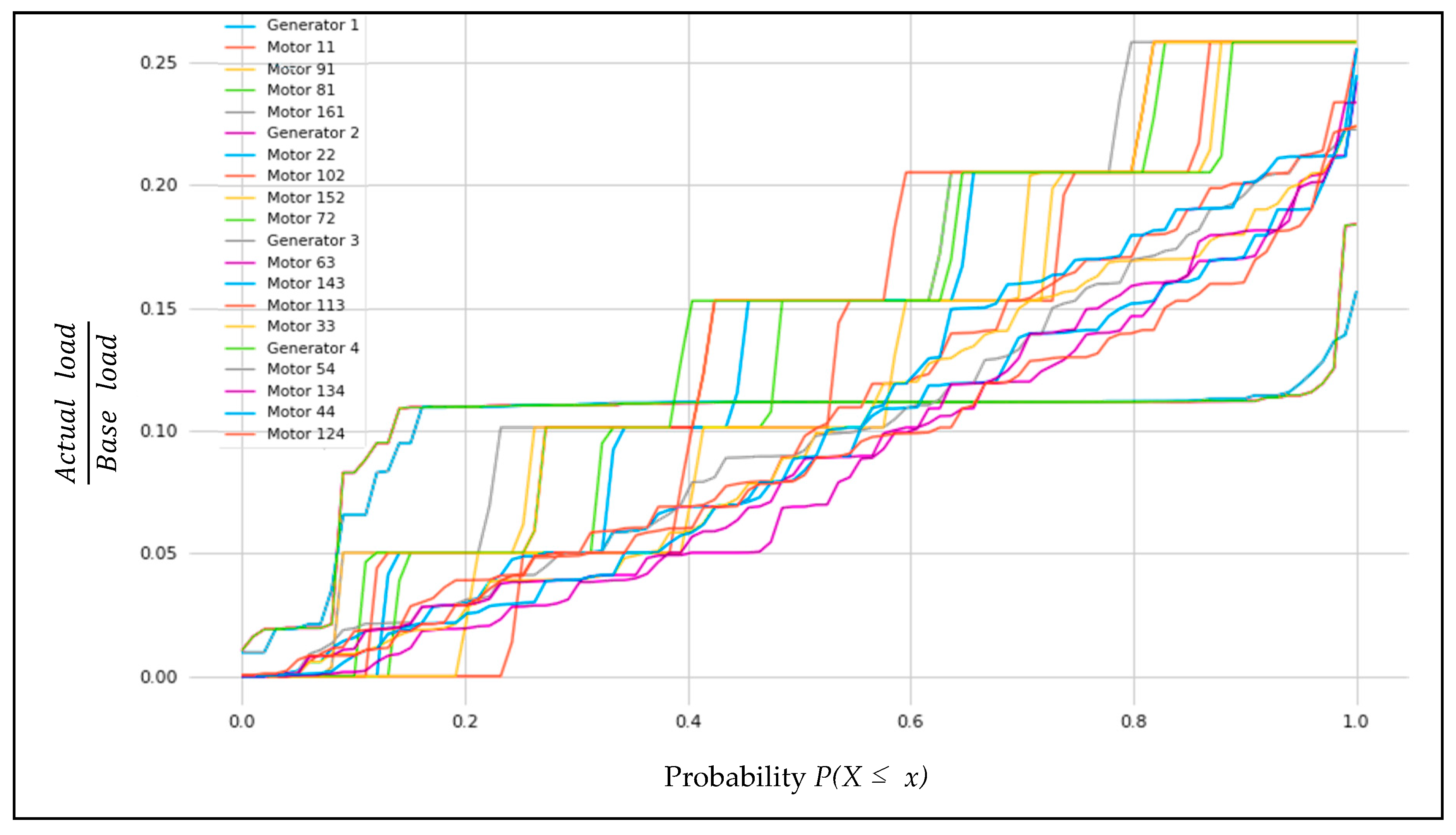
The outcomes of this analysis are shown in Figure 26, Figure 27, Figure 28, Figure 29, Figure 30 and Figure 31. The x-axis represents the probability values, and the y-axis represents the per unit (p.u.) system:

$$perunit=\frac{Actualload}{Baseload}$$

The description of these figures is as follows:

○

Every two generators were connecting to share the power demand.

○

The combination of two generators consists of the main and secondary generator.

○

The two main generators in the propulsion system have a connection to stabilise the power.

○

As there are 16 motors, the power disrupted into an optimised way depending on the flight condition by using Monte Carlo and Latin Hypercube.

○

From the optimised results, a standard deviation and cumulative distribution function was applied to estimate the probability of outcomes.

○

The cumulative distribution function should give a step-changing based on the 100 samples generated randomly with the probability between zero and one.

The explanation and discussion for the figures’ outcomes are as follows:

○

The two methods of quantitative analysis Monte Carlo and Latin Hypercube show almost the same trending in the same flight condition, which verify the given outcomes.

○

A generators trend shows a lower density for power overload.

○

Random sampling gives diversity in motor trending, which emulates the real life as they are distributed along the aircraft body.

As the MC and LH outcomes are almost identical, the motor results for the simulations with different case studies can be presented in the following

Table 3. Motor CDF results.

Motor Probabilities (RTO, TO, Cruising)
Load (%)	0	5	10	15	20	25
CDF	0	≤0.2	≤0.4	≤0.6	≤0.8	≤1

:

The MC and LH generator results also have similarities, but change, depending on the aircraft condition. The results presented in the following

Table 4. Generator probabilities.

RTO
Load (%)	0	5	10	15	20	25
CDF	0	≤0.43	≤0.64	≤0.75	≤0.83	≤0.98
TO
Load (%)	0	5	10	15	20	25
CDF	0	≤0.26	≤0.5	≤0.77	≤0.92	≤0.98
Cruise
Load (%)	0	5	10	15	20	25
CDF	0	≤0.1	≤0.15	≤0.97	-	-

are based on this condition.

In Figure 26 and Figure 27, generators and motors’ probability risk analysis gives the indication of stabile system during rolling to take off with the optimised results. The probability of distribution of generators load within the electrified propulsion grid is about 27 to 32% at max for probability function less than one from branch lauding. This is because of the flight condition of power demand. However, motors share the same power percentage in deferent probability ranges that makes the step shape.

Figure 28 and Figure 29 give the same explanation of previous figures with different flight condition. This is because of the relation between take-off and rolling to take off in terms of power density.

Cursing condition represents in Figure 30 and Figure 31 for cumulative distribution function branch load probability. The two results show the saturated probability level of generators’ power distribution. Moreover, motors were optimised to perform with half of them with normal power similar to previous conditions while the other half with minimum operation density to reduce waste in energy.

8. Conclusions

The uncertainty quantification and error estimation in the turboelectric numerical modelling processes are crucial and complex. These processes entail many crucial factors that also affect the efficiency of the system used. A turboelectric system entails sets of technical systems that must be considered when developing uncertainty quantification strategies. Different computational models can aid in the achievement of the desired outcomes because they can minimise errors. They can facilitate an active subdivision of the data and available intervals to achieve small workable intervals across a long iteration and random number systems. The subdivision of the intervals and picking of a representative interval randomly make it easy to achieve an accurate estimate. The Monte Carlo and Latin hypercube sampling techniques were demonstrated to be effective in aiding the uncertainty quantification and error estimation processes.

Moreover, the standard deviation and cumulative distribution function provide critical data convergence for error assessment and validation. By applying the uncertainty methods, the results show a desirable turboelectric system with high scalability capacity. Thus, this article demonstrates the advent of a turboelectric system that can become an essential enabler for the adoption of the MC and LH methods in the computation of the propagation of uncertainty in complex stochastic models.

References

- Felder, J.L.; Kim, H.D.; Brown, G.V. Turboelectric distributed propulsion engine cycle analysis for hybrid-wing-body aircraft. In Proceedings of the 47th AIAA Aerospace Sciences Meeting including the New Horizons Forum and Aerospace Exposition, Orlando, FL, USA, 5–8 January 2009. [Google Scholar]
- Jansen, R.H.; Bowman, C.; Jankovsky, A.; Dyson, R.; Felder, J. Overview of NASA electrified aircraft propulsion research for large subsonic transports. In Proceedings of the 53rd AIAA/SAE/ASEE Joint Propulsion Conference, Atlanta, GA, USA, 10–12 July 2017. [Google Scholar]
- Welstead, J.R.; Felder, J.L. Conceptual design of a single-aisle turboelectric commercial transport with fuselage boundary layer ingestion. In Proceedings of the 54th AIAA Aerospace Sciences Meeting, San Diego, CA, USA, 4–8 January 2015. [Google Scholar]
- Ha, T.H.; Lee, K.; Hwang, J.T. Large-scale multidisciplinary optimization under uncertainty for electric vertical takeoff and landing aircraft. In Proceedings of the American Institute of Aeronautics and Astronautics (AIAA), Orlando, FL, USA, 6–10 January 2020. [Google Scholar]
- Moody, K.J.; Replogle, C.; Rouser, K.P. Design, characterization, and integration of a turboelectric power system for small unmanned multirotor aircraft. In Proceedings of the AIAA Propulsion and Energy Forum and Exposition, Indianapolis, IN, USA, 24–26 August 2019. [Google Scholar]
- Rizzoni, G.; Hartley, T.T.; Giorgio Rizzoni, T.O.S.U. Principles and Applications of Electrical Engineering, 5th ed.; Mc Graw Hill: New York, NY, 2003; Chapter 1. [Google Scholar]
- Weinberg, L. Kirchhoff’s Third and Fourth Laws. IRE Trans. Circuit Theory 1958, 5, 8–30. [Google Scholar] [CrossRef]
- Gavin, H.P. The Levenberg-Marquardt Algorithm For Nonlinear Least Squares Curve-Fitting Problems. Dep. Civ. Environ. Eng. Duke Univ. 2013, 1–17. [Google Scholar]
- Brown, K.M.; Dennis, J.E. Derivative free analogues of the Levenberg-Marquardt and Gauss algorithms for nonlinear least squares approximation. Numer. Math. 1971, 18, 289–297. [Google Scholar] [CrossRef]
- Wallis, J.; Playford, J. A Treatise of Algebra, both Historical and Practical; University of Oxford: London, UK, 1685; Volume 15. [Google Scholar]
- Surana, K.S. Numerical Methods and Methods of Approximation in Science and Engineering; CRC Press: Boca Raton, FL, USA, 2018. [Google Scholar]
- Venkateshan, S.P.; Swaminathan, P. Computational Methods in Engineering; Elsevier Inc.: Amsterdam, The Nethetlands, 2013. [Google Scholar]
- Trias, A. HELM: The Holomorphic Embedding Load-Flow Method. Foundations and Implementations. Found. Trends® Electr. Energy Syst. 2018, 3, 140–370. [Google Scholar] [CrossRef]
- Rao, S.; Feng, Y.; Tylavsky, D.J.; Subramanian, M.K. The holomorphic embedding method applied to the power-flow problem. IEEE Trans. Power Syst. 2016, 31, 3816–3828. [Google Scholar] [CrossRef]
- Bradley, M.K.; Droney, C.K. Subsonic Ultra Green Aircraft Research: Phase I Final Report; NASA Technical Report; Boeing Research and Technology: Huntington Beach, CA, USA, 2011; p. 207. [Google Scholar]
- Bradley, M.K.; Allen, T.J.; Droney, C.K. Subsonic Ultra Green Aircraft Research Phase II—Volume I—Truss Braced Wing Design Exploration; Technical Report for NASA Technical Reports Server; Boeing Research and Technology: Huntington Beach, CA, USA, 2015; Volume I, p. 378. [Google Scholar]
- Wells, D.P.; Horvath, B.L.; McCullers, L.A. The Flight Optimization System Weight Estimation Method; NASA Technical Report; NASA Langley Research Center: Hampton, VA, USA, 2017; Volume 29. [Google Scholar]
- Salam, M.A.; Rahman, Q.M. Fundamentals of Electrical Circuit Analysis; Springer: Berlin, Germany, 2018. [Google Scholar]
- Brelje, B.J.; Martins, J.R.R.A. Electric, hybrid, and turboelectric fixed-wing aircraft: A review of concepts, models, and design approaches. Prog. Aerosp. Sci. 2019, 104, 1–19. [Google Scholar] [CrossRef]
- Palmer, J.; Shehab, E. Modelling of cryogenic cooling system design concepts for superconducting aircraft propulsion. IET Electr. Sys. Transp. 2016, 6, 170–178. [Google Scholar] [CrossRef] [Green Version]
- Koutsourelakis, P.S. Accurate uncertainty quantification using inaccurate computational models. SIAM J. Sci. Comput. 2009, 31, 3274–3300. [Google Scholar] [CrossRef]
- Schilling, R.; Lütjens, J.; Hunkel, M.; Scholl, U.; Wolf, K.; Wallmersperger, T.; Jankowski, U.; Sihling, D.; Wiegand, K.; Zöller, A.; et al. Gekoppelte FEM-Berechnungen-Ein CAE Werkzeug zur Verbesserung von crashrelevanten Karosserieteilen durch lokales Härten. VDI Berichte 2008, 143–159. [Google Scholar]
- Cunha, A., Jr.; Nasser, R.; Sampaio, R.; Lopes, H.; Breitman, K. Uncertainty quantification through the Monte Carlo method in a cloud computing setting. Comput. Phys. Commun. 2017, 185, 1355–1356. [Google Scholar] [CrossRef] [Green Version]
- Liu, C.; Si, X.; Teng, J.; Ihiabe, D. Method to Explore the Design Space of a Turbo-Electric Distributed Propulsion System. J. Aerosp. Eng. 2016, 29, 04016027. [Google Scholar] [CrossRef]
- Seaholm, S.K.; Ackerman, E.; Wu, S.C. Latin hypercube sampling and the sensitivity analysis of a Monte Carlo epidemic model. Int. J. Bio-Med. Comput. 1988, 23, 97–112. [Google Scholar] [CrossRef]
- Maier, H.R.; Tolson, B.A. Sensitivity and Uncertainty; Chapman & Hall/CRC Press: London, UK, 2008. [Google Scholar]
- Mollick, A.V. Real Exchange Rate Shocks on Tradables, Nontradables and the Current Account: Mexico, 1980–2000; Springer: Berlin, Germany, 2003; Volume 28. [Google Scholar]
- Owen, A.B. A Central Limit Theorem for Latin Hypercube Sampling. J. R. Stat. Soc. Ser. B (Methodological) 1992, 54, 541–551. [Google Scholar] [CrossRef]
- Booker, A.J. Design and Analysis of Computer Experiments; Springer: New York, NY, USA, 1998; Volume 4. [Google Scholar]
- Morgan, M.G.; Henrion, M.; Small, M. Uncertainty: A Guide to Dealing with Uncertainty in Quantitative Risk and Policy Analysis; Cambridge University Press: Cambridge, UK, 1990. [Google Scholar]
Figure 1.
Newton–Raphson method [12]. The copyright © 2014 Elsevier Inc.
Figure 2.
Electrical network architecture.
Figure 3.
Generator model prototype.
Figure 4.
Electric circuit structure and explanation.
Figure 5.
(a) exemplification of the Monte Carlo algorithm; (b) and (c) transformation from the ordinary random grid to a Latin hypercube.
Figure 6.
NASA N3-X model on GridMatch.
Figure 7.
NASA N3-X schematic system model.
Figure 8.
NASA N3-X RTO Monte Carlo branch loading average.
Figure 9.
NASA N3-X RTO Monte Carlo bus voltage average.
Figure 10.
Monte Carlo TO NASA N3-X branch loading average.
Figure 11.
Monte Carlo TO bus voltage average for NASA N3-X.
Figure 12.
Monte Carlo load average for NASA N3-X under the cruising condition.
Figure 13.
Monte Carlo bus voltage average for NASA N3-X under the cruising condition.
Figure 14.
Latin hypercube RTO load average for NASA N3-X.
Figure 15.
Latin hypercube voltage load for NASA N3-X.
Figure 16.
TO Latin hypercube branch loading average for TeDP NASA N3-X.
Figure 17.
Latin hypercube TO bus voltage average for NASA N3-X.
Figure 18.
NASA N3-X branch loading average, calculated by Latin hypercube, in the cruising condition.
Figure 19.
NASA N3-X bus voltage average, calculated by Latin hypercube, in the cruising condition.
Figure 20.
Monte Carlo standard deviation for the RTO study.
Figure 21.
Latin hypercube standard deviation for the RTO case study.
Figure 22.
Monte Carlo standard deviation for the TO case study.
Figure 23.
Latin hypercube standard deviation for the TO case study.
Figure 24.
Monte Carlo standard deviation for the cruising case study.
Figure 25.
Latin hypercube standard deviation for the cruising case study.
Figure 26.
MC RTO branch load probability.
Figure 27.
LH RTO branch load probability.
Figure 28.
MC TO branch load probability.
Figure 29.
LH TO branch load probability.
Figure 30.
MC cruising branch load probability.
Figure 31.
LH cruising branch load probability.