Article

An Analytical–Experimental Approach to Quantifying the Effects of Static Magnetic Fields for Cell Culture Applications

by
Pablo Ferrada
1,*,
Sebastián Rodríguez
1,
Génesis Serrano
2,
Carol Miranda-Ostojic
2,
Alejandro Maureira
2 and
Manuel Zapata
2
1
Centro de Desarrollo Energético Antofagasta, Universidad de Antofagasta, Av. Universidad de Antofagasta #02800, Antofagasta 1271155, Chile
2
Laboratorio de Biotecnología Ambiental Aplicada, Departamento de Biotecnología, Universidad de Antofagasta, Av. Universidad de Antofagasta #02800, Antofagasta 1271155, Chile
*
Author to whom correspondence should be addressed.
Appl. Sci. 2020, 10(2), 531; https://doi.org/10.3390/app10020531
Submission received: 14 December 2019 / Revised: 7 January 2020 / Accepted: 8 January 2020 / Published: 10 January 2020

Abstract

:
This work aimed to study the effects of static magnetic fields (SMFs) on cell cultures. A glass flask was filled with a liquid medium, which was surrounded by permanent magnets. Air was introduced through a tube to inject bubbles. Two magnet configurations, north and south, were used as perturbation. Scenedesmus obliquus and Nannochloropsis gaditana, growing in Medium 1 and 2, were subjected to the bubbly flow and SMFs. Differences between media were mainly due to conductivity (0.09 S/m for Medium 1 and 4.3 S/m for Medium 2). Joule dissipation ( P ) increased with the magnetic flux density ( B 0 ), being 4 orders of magnitude higher in Medium 2 than in 1. Conversely, the time constant ( τ P ) depended on B 0 , being nearly constant for Medium 1 and decreasing at 449 s/T for Medium 2. Dissipation occurred with the same τ P (235 s) in Medium 1 and 2 at B 0 = 0.5 T. In Species 1, the SMF effect was inhibitory. For Species 2, a higher enzymatic activity was observed. For superoxide dismutase, the relative difference was 78% with the north and 115% with the south configuration compared to the control values. For the catalase, differences of 29% with the north and 23% with the south configuration compared to control condition were obtained.

1. Introduction

Biological systems and functions usually occur in water. Thus, water is the medium where chemical reactions take place supporting life and its evolution. In addition, flows are made of fluids, which can be aqueous solutions with ions in suspension, and play a role by transporting macromolecules, among other features. Fluids can be subjected to a variety of conditions, which can be intrinsic or can be imposed perturbations. In the case of man-made externally applied forces, they are justified for practical uses either for industry in general, for biotechnological applications, or purely for research purposes. One of these external influences can be the magnetic field. Flows when coupled with magnetic or more general electromagnetic fields are described in terms of magnetohydrodynamics (MHD), which can be used for any kind of applications where fluid motion, heat, levitation, or any other effects need to be controlled. Furthermore, it provides a basis for studying the terrestrial magnetic field because of fluid motion or of magnetic field found in the sun and stars, to mention some examples. The present work involves a case study of a two-phase flow subjected to static magnetic fields (SMFs) for biotechnological applications. In the following, a brief description regarding the existence of magnetic fields in biological systems and flows is provided.
Magnetic fields in biological systems appear in several ways. For instance, magnetostatic bacterium, due to chains of single-domain biogenic magnetite, aligns its body according to Earth’s magnetic field [1]. It has been shown that birds can orient themselves to Earth’s magnetic field lines allowing their migration across long distances [2]. There are studies related to practical applications of both electric and magnetic fields in biology. For instance, cells can exhibit directional migration or alignment upon exposure to static electric fields [3]. Authors have differentiated cells by applying external magnetic fields established by permanent magnets [4]. This is based on the equilibrium between the magnetic gradient force and gravity, and on the magnetic fingerprint of each type of cell. In addition, a magnetic trap for living cells in a buffer has been developed. To obtain the movement of cells towards zones of magnetic field minima, the original medium was enriched with a paramagnetic fluid to achieve a magnetic susceptibility much higher than that of the cells [5]. Further procedures to supervise cells have been developed; for instance, researchers have created nanomushroom structures as labelfree nano sensors for long-term cell proliferation detection [6]. In more detail, magnetic fields can participate at several levels, ranging among the tissue, cell, membrane, and molecular levels [7]. In this regard, it has been stated that magnetic fields can alter the rate, yield, and product distribution of chemical reactions [8]. Reviewing the effects of SMFs on cellular systems, authors point out that the radical pair recombination and the diamagnetic anisotropy can lead to changes and subsequent effects on the susceptibility of biomolecules, intracellular structural modifications, and changes in the enzymatic reactions [9].
To elucidate how fields act on cells, main processes in cells must be understood first. The main physiological processes in cells generate reactive oxygen species (ROSs). In case of microalgae, ROSs are generated by mitochondria, chloroplasts, and peroxisomes [10,11]. ROSs can oxidize essential macromolecules, as they are highly reactive. Cells exhibit an antioxidant defense system that neutralizes or metabolizes ROSs. This defense system comprises antioxidant enzymes, such as catalase, superoxide dismutase, ascorbate peroxidase, and glutathione peroxidase, among others, and low-molecular-weight metabolites such as glutathione, ascorbic acid, carotenes, phenols, and flavonoids [12]. When this defense system is overcome, the equilibrium shifts to a pro-oxidant situation, and a state of oxidative stress is established in which oxidative damage occurs to proteins, nucleic acids, and lipids [13]. Environmental factors and the ingress of contaminants into the cells can intensify the production of these molecules, where the most damaging is the superoxide anion (O2), the hydrogen peroxide (H2O2), and the hydroxyl radical (OH) [14,15]. ROSs can be classified into two categories: free radicals and non-radical species [16]. Free radicals are molecular species, containing an unpaired electron in an atomic orbital [17]. Due to the unpaired electron, these molecules are paramagnetic and susceptible to magnetic fields. As a result, a radical will tend to take an electron from stable molecules to achieve its electrochemical stability, so they are highly reactive. Based on this definition, oxygen and hydrogen atoms, as well as transition metals, are free radicals [18]. All these processes usually occur in a watery context, so water is the object of study when magnetic fields are present.
As stated above, magnetic fields can directly impact biological systems; however, these effects can be caused due to modifications in the medium where cells grow. Therefore, an understanding of what changes are experimented in water when exposed to magnetic fields is necessary. There are several studies regarding the effects of magnetic fields on water. For instance, a higher evaporation rate has been found [19]. Authors [20] have reported that viscosity, surface tension, and vaporization enthalpy are properties that are correlated with intermolecular forces, which are given by hydrogen bonds in water. Thus, the changes experimented though these properties can be described by studying these forces. Water, when exposed to magnetic fields, was found to be more stable, showing less molecular energy and more activation energy [21]. It has been stated that the variation in molecular energy is an indicator of the reorientation or formation/breaking of hydrogen bonds [22]. An increase in the amount of hydrogen bonds and a decrease in the self-diffusion coefficient of water molecules were linked to tighter bonding and more stability in water subjected to magnetic fields [23]. Some research [24] has shown that surface tension increased with magnetic field intensity [24]. For water containing minerals, the evaporation rate from electrolyte solutions (water with NaCl, KCl, Na3PO4, and CaCl2) was a function of the ordering or disordering role of the cations and anions present [25]. The dissolution of oxygen was also affected by magnetic fields. It was found that the equilibrium concentration of paramagnetic oxygen did not change; however, the dissolution rate increased. This result was explained by a magnetically higher convection in water due to the inhomogeneous magnetic susceptibility produced by the dissolution of oxygen in water [26].
A closer look into the description of fluids, which includes water, will allow for an approach to study systems under different conditions. A fluid is represented by phases, which can be liquid or gaseous and contain solid material. It is common to find multiple phases coexisting simultaneously. A clear example can be the transport of hydrogen or liquefied gas [27]. To understand the behavior of a multiphase fluid, it is necessary to understand how the fluid interacts as a fraction of liquid and gas under fluid conditions. The multiphase flow is generally represented by a channel that can be in four flow regimes, each determined by the velocity of the fluid and the concentrations of liquid and gas. Each regime varies according to the increase in concentration of gas in the fluid. For a variety of cases, the lowest gas concentration called the bubble regime is used [28]. The analytical method for multiphase fluid is represented by Navier-Stokes (N-S) equations coinciding with those of an incompressible fluid, where the numerical solutions show the desired phenomenon. These expressions lead to the continuity and balance equations of momentum for a two-phase fluid [29].
Multiphase fluids can be studied by simplifying N-S equations and adapting to the requirements of the case. Current computer capabilities require reducing the error when writing codes for the development of mathematical models that are increasingly simpler to process. There are great exponents that suggest simplified methods for given physical conditions of the fluid. On the one hand, Euler’s approach proposes that, considering the particle density and the gas volume faction, each phase of the fluid can be studied separately if it is assumed that each phase can be represented as continuous and inter-penetrating. In addition, they coexist, separated by an interface [30]. On the other hand, the bubble fluid method is a simplification of Euler’s, since it considers that the density of the gas present is less than 10% of the total volume of the fluid. Both phases are subjected to the same pressure field. Unlike other models, this treatment allows for an efficient study of a two-phase fluid as if it were one, that is to say, one set of N-S equations is used and subsequently the volume fraction is split in two, for each phase [31]. If the need is to study the average phase concentration, the assumption that the density of each phase is constant allows for use of the mixing method. It is very similar to the bubble fluid method, with the difference that the mixing method also covers liquid or solid drops immersed in the fluid. The theoretical knowledge and the previous experimental studies on magnetic fields in biological systems enables the development of methodologies for biotechnological applications. Accordingly, the aim of the research is as follows.
This work focuses on cell cultures inside a glass flask, containing a liquid medium in which air is introduced through a tube, and affected by external SMFs. We consider that magnetic fields can affect water properties as well as biological media by means of modifying the equilibrium between ROSs and antioxidant molecules, promoting either beneficial or negative conditions. Therefore, cells can activate their defensive system in response to an external agent. In this context, this research relates physical properties of the medium with the magnetic field, discusses the effects of the magnetic field by evaluating solutions, and performs experimental measurements quantifying the production of antioxidants.
Finally, the cell cultures used in this work correspond to the Scenedesmus obliquus and Nannochloropsis gaditana microalgae. These model species feature a known structure, functionality, and rapid growth. These characteristics can provide effectiveness regarding the effects of SMFs. They present biotechnological potential for the generation of antioxidant biomolecules such as β-carotenes in S. obliquus or the high accumulation of polyunsaturated fatty acids (PUFAs) in N. gaditana.

2. Theory

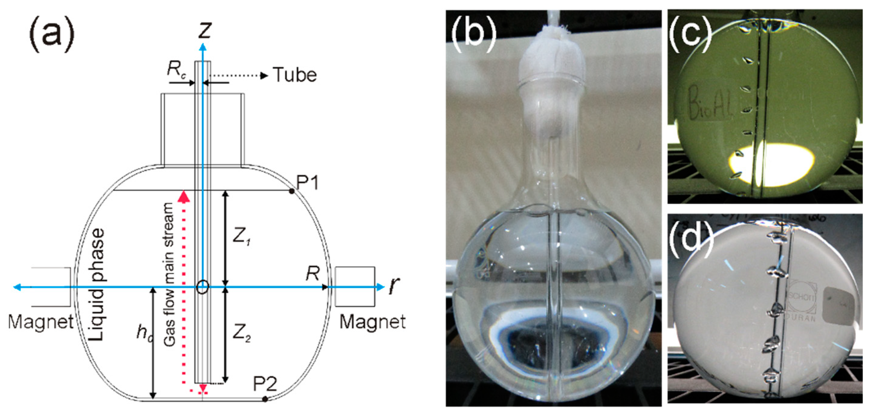
2.1. General Description

Air is introduced near the bottom of a glass flask though a thin tube resulting in bubbles (Figure 1). Bubbles exhibit buoyancy, inducing fluid circulation in the medium. Consequently, there are two flows to consider: air as gas and water as a liquid phase. One possible problem statement for the multiphase flow case is using two sets of N-S equations, accounting for the two flows and described by the continuity and momentum balance. A simplified formulation is possible when the following assumptions can be undertaken: the air density is much lower than the liquid density (the ratio of air and water density is ~0.001 for 20   ° C < T < 40   ° C ), the balance between drag and pressure forces determines the motion of bubbles arising from air inflow in the flask relative to liquid, and the pressure is valid for the two phases. Thus, the momentum conservation and continuity equation are expressed by Equations (1) and (2), where the subscript l stands for liquid and g for gas.

2.2. Problem Statement

The general problem is described by the volume-averaged incompressible, transient N-S equations involving two phases, liquid and gas. In compact form, it can be expressed by Equation (1), where u l = ( u l , v l , w l ) is the liquid phase velocity with components u l ,   v l , and w l . The pressure, dynamic viscosity of the liquid medium, density of the liquid medium, and gravitational acceleration are denoted as p , μ l , ρ l , and g . The last two terms at the right side of Equation (1) stand for the gravitational force and an extra external force to be described in Section 2.1, due to the presence of a permanent magnet. The continuity equation is expressed by Equation (2). The quantities Φ l and Φ g are the liquid and gas phase volume fractions, respectively, for which Φ l + Φ g = 1 .
Φ l ρ l u l t + Φ l ρ l ( u l · ) u l = p + Φ l μ l 2 u l + f g + f m
t ( Φ l ρ l + Φ g ρ g ) + · ( Φ l ρ l u l + Φ g ρ g u g ) = 0
Developing the N-S equation in cylindrical coordinates leads to equations for the radial ( r ), circumferential ( θ ), and axial ( z ) components. Thus, Equation (3) corresponds to r , Equation (4) to θ , and Equation (5) to z -components. In general, the dynamic viscosity ( μ ) is related to the kinematic viscosity ( ν ) as μ = ρ ν . The total external volume force is denoted as f = ( f r , f θ , f z ) = f g + f m , where the gravitational volume force is written as f g = Φ l ρ l g e ^ z .
Φ l ρ l u l t + u u l r + v r u l θ v l 2 r + w u l z = p r + Φ l μ l [ r ( 1 r ( r u l ) r ) + 1 r 2 2 u l θ 2 2 r 2 v θ + 2 u l z 2 ] + f r
Φ l ρ l v l t + u v l r + v l r v l θ + u v l r + w v l z = 1 r p θ + Φ l μ l [ r ( 1 r ( r v l ) r ) + 1 r 2 2 v l θ 2 + 2 r 2 u l θ + 2 v l z 2 ] + f θ
Φ l ρ l w l t + u w l r + v r w l θ + w l w l z = p z + Φ l μ l [ 1 r r ( r w l r ) + 1 r 2 2 w l θ 2 + 2 w l z 2 ] + f z

External Applied Magnetic Field

When an external magnetic field is applied, the general treatment of the fluid flow requires the consideration of charge carriers in the medium. Ionic species will be transported by the fluid flow, which are subjected to an SMF. The induced current due to the external B leads to the extra force of the form expressed in Equation (12), whose components need to be included in Equation (1). To determine the regime under which the interaction between the magnetic flux density B and the medium occurs, the magnetic Reynolds number ( R e m ) is introduced. It is defined in Equation (6), quantifying the ratio of advection to diffusion of B , where λ = ( μ 0 σ ) 1 is the magnetic diffusivity, μ 0 the magnetic permeability of vacuum, and σ is the fluid conductivity. For R e m 1 , a diffusion regime dominates, meaning that B -field lines are determined only by BC and not the fluid flow. Conversely, for R e m 1 , an advection regime governs, meaning that B -field lines follow the fluid.
R e m = U L λ
Considering the R e m 1 case, let E 0 , J 0 , and B 0 be the fields when u l = 0 , and let e , j, and b be the infinitesimal perturbation in E , J , and B , which are produced due to the velocity u l transporting ionic species. These considerations lead to the following coupled equations, noting that this work is constrained to SMFs, i.e., × E 0 = B 0 / t = 0 . Since E 0 is irrotational, it can be expressed as E 0 =   V . The extra contribution u l × b in Equation (8) was not considered. From Equation (7), it can be shown that | e | / L   ~   | b | / t . In addition, | b | ~ | B 0 | R e m [32], so e   ~   U | B 0 | R e m . Therefore, e can be neglected in Equation (8), which, in combination with Equation (7), results in the current J 1 in Equation (10). If there are no external electric fields applied, J 0 = 0 , leading to Equation (11). The form of this current reveals that, under the condition of R e m 1 , B influences the velocity field u l ; however, there is little influence of u l on B . The final form of the Lorentz force is expressed in Equation (12) [33].
× e = b / t
j = σ ( e + u l × B 0 )
J 0 = σ   E 0
J 1 = j + J 0 =   σ (   V +   u l × B 0 )
J = σ ( u l × B 0 )
f m = J × B 0

2.3. Solution Strategy

This work focuses on the case where two components of u l are zero and the z -component of the liquid phase velocity is r -dependent as well as t -dependent. Thus, w l = w l ( r , t ) and u l = w l ( r , t ) e z . This consideration is based on experimental observation (Section 3) and numerical simulations [34,35]. The medium temperature is fixed ( T is constant). The external imposed field is assumed to be homogeneous and expressed as B 0 = B 0 e ^ r , according to the location indicated in Figure 1, with B 0 a real positive constant. In addition, the low R e m applies. Using Equations (11) and (12), the current and the Lorentz force become J ( r , t ) = σ B 0 w l ( r , t ) e ^ θ and f m ( r , t ) = σ B 0 2 w l ( r , t ) e ^ z . The pressure is expressed as p ( z ) = ϕ l ρ l g z , leading to p / z = ϕ l ρ l g , and the expression p / z Φ l ρ l g in Equation (5) is considered to be ~0. This formulation allows for a time-dependent study.

2.3.1. Velocity for the Liquid Phase

Replacing the liquid phase velocity, current, and force in Equations (3)–(5) results in Equation (13), a unique equation in which the kinematic ( ν l ) viscosity, the liquid volume fraction ( ϕ l ), the fluid density ( ρ l ), and the magnetic flux density B 0 appear as constants.
w l ( r , t ) t = ν l 2 w l ( r , t ) z 2 + ν l 1 r w l ( r , t ) r σ ϕ l ρ l B 0 2 w l ( r , t )
Expressing the liquid phase velocity as w l ( r , t ) = F ( r ) G ( t ) and computing its partial derivatives to be introduced in Equation (13), w l / t = F G ˙ , w l / r = G F and 2 w l / r 2 = G F . This process leads to Equation (14).
F G ˙ = ν l G F + ν l 1 r G F σ ϕ l ρ l B 0 2 F G
All terms in Equation (14) can be multiplied by 1 / ( F G ) . In addition, the proportionality factor η is introduced. Thus, Equation (15) can be solved by separation of variables.
G ˙ G = ν l F F + ν l 1 r F F σ ϕ l ρ l B 0 2 = η 2
The solution for the time-dependent function G is direct, resulting in Equation (16), where A is a real constant.
G ( t ) = A e η 2 t
Rearranging Equation (15), one obtains Equation (17).
r 2 F + r F + ( η 2 ν l σ ϕ l μ l B 0 2 ) r 2 F = 0
Defining β 2 =   (   η 2 / ν l σ / ( ϕ l μ l ) B 0 2 ) , the solution to Equation (17) can be found in terms of the Bessel functions J 0 and Y 0 , where J 0 is the Bessel function of the first kind, and Y 0 is the Bessel function of second kind, with C 1 and C 2 as constants to be found (Equation (18)).
F ( r ) = C 1 J 0 ( β   r ) + C 2 Y 0 ( β   r )
Considering J 0 ( β   r ) and Y 0 ( β   r ) when r 0 , the constant accompanying Y 0 is chosen to be zero as Y 0 diverges, leading to Equation (19), where C 1 = C is a real constant. The z -component of the velocity is expressed in Equation (20).
F ( r ) = C 1 J 0 ( β   r )
w l ( r , t ) = C J 0 ( β   r ) e   η 2 t
Setting the boundary condition w ( R , t ) = 0 leads to J 0 ( β   R ) = 0 , meaning that β k   R = γ k , where the γ k values are the zeros of J 0 for k = 1 ,   2 ,   3 . It follows that β k 2   R 2 = γ k 2 ; thus, R 2 (   η 2 k / ν σ B 0 2 / ( ϕ l μ ) ) = γ k 2 . It is noticed that β k 2 is always positive as γ k 2 > 0 holds. Solving for   η 2 k , one obtains Equation (21), where the terms at the right side of the equation are associated to viscous and magnetic damping, respectively.
η 2 k = ν l R 2 ( γ k 2 + R 2 σ B 0 2 ϕ l μ ) = ν l ( β k 2 + σ B 0 2 ϕ l μ )
Setting the initial condition w ( r , 0 ) = W 0 leads to Equation (22), which is based on the orthogonality properties of Bessel functions [36,37].
w l ( r , t ) = 2 W 0 k = 1 J 0 ( β k   r ) β k R J 1 ( β k R ) e η k 2 t

2.3.2. Power Dissipation

An equation accounting for power dissipation via the Joule effect has been obtained [38]. This process gives rise to an increase in thermal energy and the corresponding fall in kinetic energy. In this case, volume fraction ϕ l and ϕ g must be incorporated. Revisiting the inviscid equation [39], Equation (23) considers the volume fraction of the liquid. The term at the left side in Equation (23) is the material derivative D / D t = d / d t + ( u · ) u , with u the velocity.
D D t ( Φ l ρ l u l ) = p + J × B 0
Multiplied by u l (the fluid velocity), in the sense of a dot product, Equation (23) leads to Equation (24).
D D t ( Φ l ρ l u l 2 2 ) = ( J × B 0 ) · u l · ( p u l )
Rearranging terms allows us to write Equation (24) as follows.
D D t ( Φ l ρ l u l 2 2 ) = J · ( u l × B 0 ) · ( p u l )
Using Equation (11) in the form of u l × B 0 = J / σ in Equation (25) and integrating over the entire volume leads to Equation (26). The volume integral of ρ l u l 2 / 2 is the global kinetic energy ( Ξ ).
D D t V ρ l u l 2 2 d V = D D t Ξ = 1 σ Φ l J 2 d V
The kinetic energy can be approximated by solving Equation (27), where l is the characteristic length scale for the flow (parallel to the magnetic field), and l m i n is the smallest eddy size in a turbulent flow. The solution is expressed in Equation (28) [40]. This equation anticipates that, provided l m i n and l maintain the same order, the flow will be annihilated on a time scale τ . The dissipation is subject to the constraint that neither the creation nor the destruction of linear momentum is possible. This phenomenology has been treated in [41], where the discussion is centered in the properties of fluids moving in a uniform magnetic field, showing that the component parallel to the magnetic field is conserved while the normal components decay exponentially.
D D t Ξ = ( l m i n l ) 2 D t τ
Ξ ( t ) = Ξ 0 e ( l m i n l ) 2 t τ
Denoting P , the power dissipation via the Joule effect, as P = J 2 d V / ( σ Φ l ) and using J = σ B 0 w l ( r ) e ^ θ in Equation (28) (Section 2.3), the magnitude of the power dissipation can be found via Equation (29), meaning that the higher the conductivity, the higher the volume fraction of the liquid. Moreover, the higher the fluid velocity is, the higher the magnitude of the power dissipation through the Joule effect becomes. The volume can be expressed in terms of the generic r -coordinate, i.e., V = V ( r ) , so the volume element d V is r -dependent.
| P ( t ) | = σ B 0 2 Φ l V ( r ) w l ( r , t ) 2 d V
To use Equation (29), the domain corresponding to the portion of the flask where the fluid is circulating and the power is dissipated must be found. It can be obtained by defining the total volume V as the volume of a sphere of radius r ( V 0 = 4 π r 3 / 3 ) minus the volume of the top ( V 1 ) and bottom ( V 2 ) cap, defined by the water level and the geometry at the bottom of the flask, and minus the volume of the part of cylinder inside the flask ( V 3 ) though which air is introduced. Thus, V = V 0 ( V 1 + V 2 + V 3 ) , and the volume element d V can be expressed in terms of the r -coordinate. It can be demonstrated that d V = [ 4 π r 2 π ( h 1 2 + h 2 2 ) 2 π l r ] d r with h 1 = R Z 1 and h 2 = R h 0 , where Z 0 is the distance measured from the origin of the reference system to the top water level, and h 0 is the depth measured from the origin of the reference system to the bottom of the flask (see Figure 1). The length of the cylinder inside the flask has a length l = Z 1 + Z 2 and an external radius R c . The power dissipation is rewritten in Equation (30), which depends on the function describing the velocity of the liquid phase.
| P ( t ) | = σ B 0 2 Φ l ( 4 π 0 R w l ( r , t ) 2 r 2 d r π h 1 2 0 ( R 2 Z 1 2 ) 1 / 2 w l ( r , t ) 2 d r π h 2 2 0 ( R 2 h 0 2 ) 1 / 2 w l ( r , t ) 2 d r          2 π l 0 R c w l ( r , t ) 2 r   d r )

3. Materials and Methods

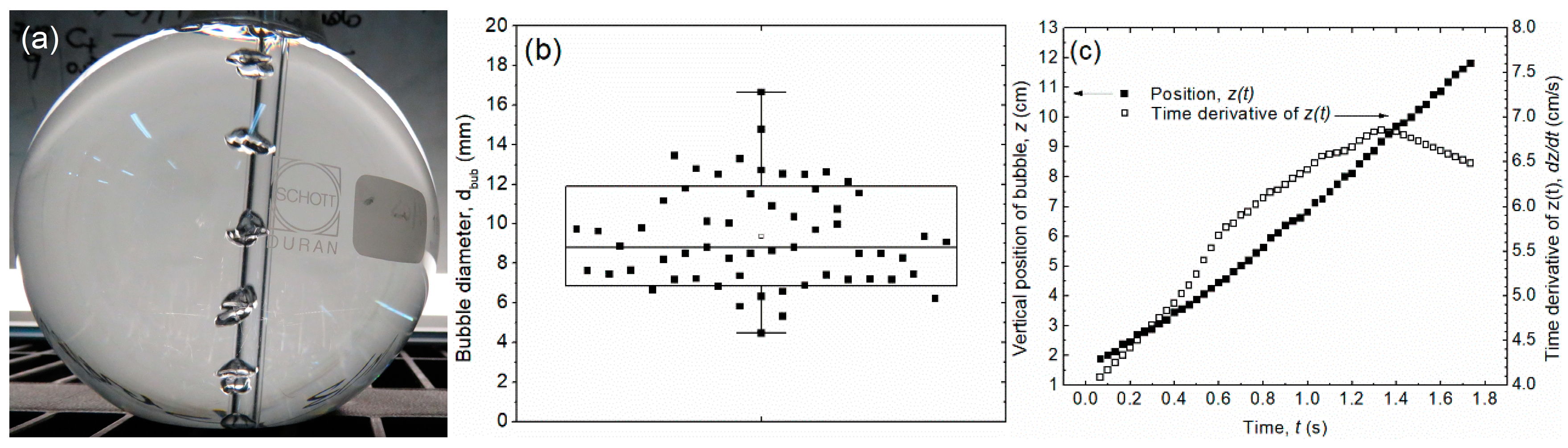
3.1. Setup 1: Bubbles

To determine bubbles’ diameter and their speed, a setup consisting of 4 different flasks filled with fresh water was mounted. For each flask, air was introduced by a tube, which resulted in bubbles, as Figure 2a shows. Photographs and video in slow motion mode were taken for each individual flask, as bubbles were rising. The bubble diameter was obtained, as the dimensions of the flask were known, and distances were thus related to pixels (see Appendix A), whereas the vertical component of the bubble velocity was computed by processing video frames with PhysMo Video Motion Analysis software determining the bubble position as a function of time (Videos can be found in the Supplemental Materials).
According to the measurements of bubble diameter d i (with i , the i -th measured diameter) and using ϕ g = i = 1 n d i 3 / ( 6 R 2 L ) [42], the gas volume fraction becomes ϕ g = 0.022   ± 0.001, meaning that ϕ l = 0.978   ± 0.001. An expression, Equation (31), accounting for the motion of bubbles in vertical tubes of arbitrary cross sections was investigated in [43]. It requires the perimeter Π = 2 π R 0 defined by the tube internal radius R 0 . This equation can be used to determine a representative value for the bubble vertical velocity. By choosing values for the tube as R 0 = 2 mm and the measures of the flat-bottom flask as l = Z 0 + h 0 with h 0 = R cos [ arctan ( W / D ) ] , W = 60 mm, and D = 2 R = 131 mm, the magnitude of the vertical bubble velocity becomes U b = 7 cm/s (compare with the experimental value in the right axis of Figure 2c).
U b = ( 8 π ) 1 / 2 g Π

3.2. Setup 2: Cultures

3.2.1. Biological Material and Culture Conditions

Two microalgae species were cultured, Scenedesmus obliquus (S. obliquus) and Nannochloropsis gaditana (N. gaditana). The culture medium for S. obliquus was the bold basal medium (BBM) [44,45], prepared from fresh water. The medium for N. gaditana was a modified f/2 [46], prepared from sea water. In this work, BBM is denoted as Medium 1, and f/2 as Medium 2. The experiment was performed under phototroph conditions using fluorescent lamps, which provide an intensity of 120 μmolm−2s−1, at 23 °C. The cultures were prepared in flasks of 1000 mL with constant air inflow through a tube (see Figure 3). Main characteristics of Species 1 and 2 are summarized in the following:
  • Species 1 is a freshwater microalga belonging to the Chlorophyceae class. It is immobile and forms aligned colonies. It is mainly characterized by the absence of a rigid cellular wall, which is made of polysaccharides. The cell is included in a thin and elastic plasma membrane in a mucilaginous envelope [47]. It also has a great biotechnological interest due to the high production of antioxidant compounds such as lutein [48].
  • Species 2 is a marine microalga belonging to the Eustigmatophyceae class. It does not exhibit flagella. Its cell wall is smooth, allowing a greater thickness and resistance. Its main characteristics are a rapid growth and large accumulation of polyunsaturated fatty acids (PUFAs) [49,50].

3.2.2. Exposure to External Static Magnetic Fields

Cultures were exposed to SMFs, implemented in an array of 4 neodymium magnets, each one providing 5000 G and forming a ring. This intensity was measured with an AC/DC magnetic meter PCE-MFM 3000. The magnets were placed using two different magnet configurations: (i) all north (N) poles pointing the center; (ii) all south (S) poles pointing the center of the flask. In addition, the application of SMFs was implemented in the following way. The culture in the exponential growth phase was exposed to SMFs for 1 h every day for 5 days. Accordingly, the effects of SMFs on the cultures were measured every 24 h, for 5 days. To evaluate results, cultures were prepared in triplicate, comparing the 3 samples exposed to SMFs for a given configuration (N or S) with a control sample without exposure to SMFs. See Table 1.

3.2.3. Physicochemical Parameters

To determine the physicochemical parameters such as pH, temperature, salinity, and dissolved oxygen (DO), the multiparameter probe HI 98194 (Hanna instruments) was used. For this purpose, an aliquot of 50 mL was taken from both types of cultures, the control and the treated samples. Data were recorded for 5 days every 24 h. The temperature for Medium 1 and 2 was maintained at 20 °C with a standard deviation below 2 °C, over the whole period. Medium 1 had a 7% lower pH over time compared with Medium 2. Regarding the electrical conductivity, Medium 1 exhibited σ = 0.09 ± 0.1 S/m, whereas the measurement for Medium 2 was σ = 4.3 ± 0.3 S/m. The salinity of water corresponding to Medium 1 was 0.5 ± 0.1 psu. In the case of Medium 2, this value was 27.7 ± 2 psu. The concentration of DO in Medium 1 was higher than in Medium 2 with a value of 6.4 ± 0.3 mg/L compared to 5.1 ± 0.2 mg/L. Table 2 summarizes the values for numerical evaluation.

3.2.4. Enzymatic Activity

For the determination of the enzymatic activity of superoxide dismutase (SOD) and catalase (CAT), 10 mg of lyophilized sample of each microalga was used. The cell break was performed in a mortar with liquid nitrogen and glass beads. The homogenization was performed with 2 mL of extraction buffer (K2HPO4-KH2PO4) KH2PO4, 50 mM, pH 7.0, containing Triton X-100 (0.01% v/v) [53]. Subsequently, the homogenate was centrifuged at 13,000 G at 4 °C for 15 min [54]. Protein quantification was performed according to the Bradford method [55]. The extract was immediately used to quantify the activity of antioxidant enzymes.
The enzymatic activity was measured for both microalgae in terms of SOD based on the photochemical reduction of Nitro blue tetrazolium chloride (NBT) described by [54,56] and modified. The catalase activity was evaluated through spectrophotometry by the disappearance of hydrogen peroxide according to [57]. The biological characterization presented in Section 4.3. was subjected to an analysis of variance (ANOVA) with a confidence of 95%, using the Minitab 17 software.

3.2.5. Carotenoid Quantification

The high-performance liquid chromatography (UHPLC) method used for the quantitative identification of carotenoids present in both microalgae species was based on the protocol described by [58]. The separation and chromatographic analysis were performed on a DIONEX ULTIMATE 3000 chromatograph with a diode array detector, connected to an ORBITRAP Q EXACTIVE FOCUS (Thermo Scientific). The results were analyzed using Thermo Xcalibur Sequence Setup software.

4. Results and Discussion

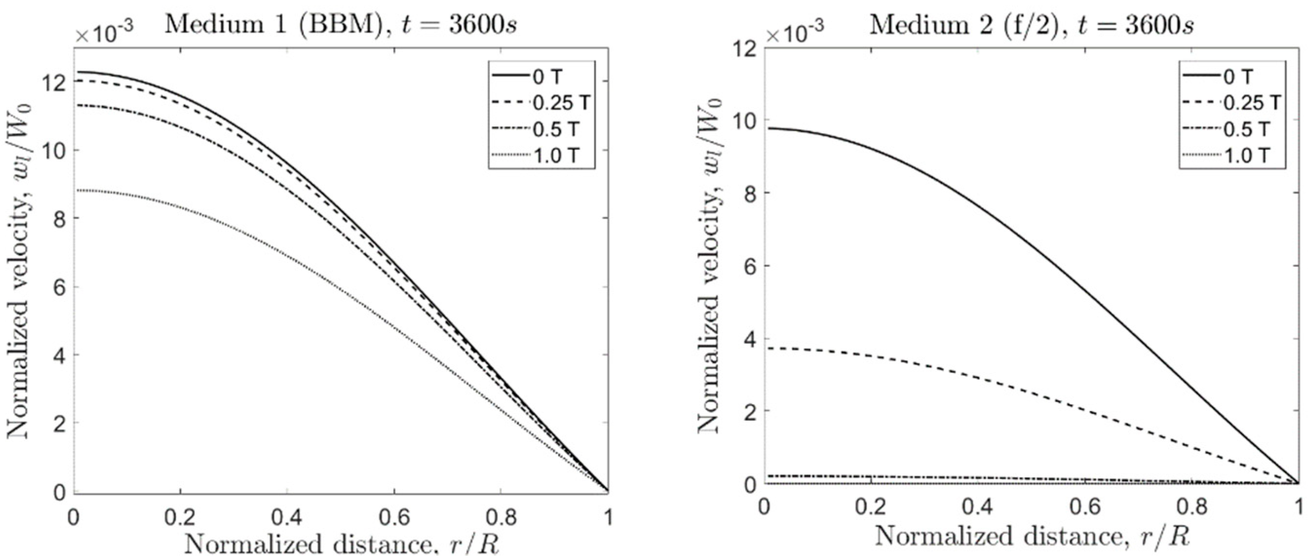
4.1. Liquid Velocity for Different Media with Varying B 0

The evaluation of Equation (24) using parameters for Medium 1 (BBM) and Medium 2 (f/2) led to the direct comparison of the impact of different values for the magnetic flux density B 0 at different times in terms of the velocity for the liquid phase. The chosen B 0 values correspond to 0 T (no applied external magnetic field), 0.25 T (close to the practical value obtained in the laboratory), 0.5 T (the datasheet value of N33 grade Nd magnets), and 1 T (close to the maximal possible value for permanent magnets). Likewise, the evaluation was performed at 10 s, 450 s (7.5 min), 900 s (15 min), and 3600 s (1 h) (Figure 4).

4.1.1. Medium 1

At the initial stage ( t = 10 s), the normalized velocity ( w l / W 0 ) in Medium 1 was independent of B 0 . At t = 450 s, w l / W 0 decreases ~20% from the original value, not showing a great dependency of the magnetic flux density. Only for B 0 = 1 T, the w l / W 0 value was slightly lower than the no-field condition (4.1% lower). For longer times (at t = 900 s, 1800 s, and 3600 s), the w l / W 0 ratio became more affected by B 0 . At the latest evaluated time ( 3600 s), the normalized velocity decreased 28.3% at 1 T with respect to the no-field condition.

4.1.2. Medium 2

Conversely, the normalized velocity w l / W 0 showed the dependency of the magnetic flux density already at the initial stage ( t = 10 s), where for B 0 = 1 T, the ratio w l / W 0 decreased by 4.2% with respect to the no-field condition. For longer times, the w l / W 0 value in Medium 2 decreased approximately by the same amount as in Medium 1 for the no-field condition. However, comparing at equal times, the normalized velocity decreased faster compared to Medium 1 with increasing B 0 . For instance, at t = 450 s, the w l / W 0 value in Medium 2 dropped by 11.4% for B 0 = 0.25 T, 38.3% for B 0 = 0.5 T, and 85.5% for B 0 = 1 T (absolute differences). In Medium 1, the w l / W 0 ratio varied less than 5%, even for B 0 = 1 T at t = 450 s. This situation was repeated for 900 s and t = 1800 s. In Medium 2, the decrease in w l / W 0 was much more pronounced for increasing B 0 values compared to the reduction of the w l / W 0 value in Medium 1.

4.2. Power Dissipation

The power dissipation was numerically evaluated using the velocity of the liquid phase (Equation (24)) in Equation (30) and the values found in Table 2 as well as the geometrical parameters indicated in the experimental procedure section. To investigate the effects of B 0 on the response time for the power dissipation in Medium 1 and 2, the same initial value of the fluid velocity W 0 was considered for both media. The numerical evaluation shows that the magnitude of P decreases exponentially with time, as expressed by Equation (32), where τ P corresponds to the time constant, i.e., the time for which P has reduced by a factor of 0.6321. This form is linked to Equation (30), where the kinetic energy is expressed as an exponential function. Thus, Figure 5a,b show the normalized power dissipation as a function of time (the insets depict the time in logarithmic scale). The integration was performed between 0 and 3600 s. Figure 5c shows the computed time constants as a function of the magnetic flux density for Medium 1 and Medium 2. The information provided is summarized in Table 3 and Table 4.
| P ( t ) | = P 0 e t / τ P
Table 3 and Table 4 show the impact of the magnetic flux density on the time constant of the power dissipation within Medium 1 and Medium 2, respectively. While the power dissipation in Medium 2 is 4 orders of magnitude larger than in Medium 1 and increases with the applied external magnetic flux density, the time constant decreases with B 0 for both media. Conversely, the time constant for Medium 1 remains nearly constant, decreasing at a rate of 17.8 s/T, whereas the time constant for Medium 2 decreases at a rate of 449 s/T. It was observed that for low B 0 values, power dissipation in Medium 1 is faster than in Medium 2. On the contrary, for high B 0 values, dissipation in Medium 2 becomes faster. The latter means that there is a specific B 0 value at which the power dissipation in Medium 1 and 2 occurs with the same time constant. According to Figure 5c, this condition is found when B 0 ~ 0.5 T, leading to τ P ~ 235 s.

4.3. Effects at Biological Level: ROS

The enzymatic activity in terms of the superoxide dismutase (SOD) was measured after magnetic field exposure and shown in Figure 6a for species 1 and in Figure 6b for species 2. For Species 1 (S. obliquus), the application of SMFs resulted in 26 and 50% less SOD activity relative to the control values for the north and south configurations, respectively. On the contrary, in the case of Species 2 (N. Gaditana), SOD increased significantly with the SMF treatment reaching a maximum of 1.22 mUmg−1 with the north and 1.593 mUmg−1 with the south configuration, meaning significant relative differences of, respectively, 78 and 115% above their control values. In terms of the catalase (CAT) in Figure 7, Species 1 showed 14 and 7.6% less CAD activity compared to the control values for the north and south configurations, respectively. Conversely, Species 2 experimented with changes under SMFs as the CAT levels increased up to 0.13 mUmg−1 with the north and 0.13 mUmg−1 with the south configuration, meaning, respectively, relative differences of 29 and 23% with respect to their control conditions.
The quantification of metabolites of interest was measured after 96 h of SMF exposure. Figure 8A shows a slight decrease in the production of violaxanthin and lutein with respect to the control (<1%). Figure 8B shows that the abundance of violaxanthin increased by 40.9% compared to the control.
The results obtained in terms of the enzymatic activity show a clear difference between both microalgae species. In the case of Species 2, SOD increases significantly with respect to the control in both magnet configurations. This behavior can be associated to the oxidative stress that SMFs are causing to the cell culture [59]. Medium 2, being ~50 times more conductive than Medium 1, could promote a more effective electron transfer and allowing for a more pronounced ROS formation. In addition, a very important aspect is the structure of the cell. Since it has a rigid wall, it becomes less susceptible to the damage caused by ions, which are driven by magnetic field gradients. The antioxidant defense machinery counteracts the damage by activating antioxidant enzymes such as SOD first and then the non-enzymatic antioxidants such as pigments. The analysis of carotenoids after 96 h of SMF exposure shows a clear increase in violaxanthin with respect to the control, revealing the action of the defense of the cell against ROS oxidative stress [56,60].
On the contrary, in the case of Species 1, there is a significant inhibition of SOD with respect to the control. To explain the behavior of the enzyme for these cells, we can hypothesize several points. (i) SODs are metalloproteins that catalyze the dismutation of O2 to H2O2 and O2 [53,61,62]. Depending on the transition metal found in its active site, SODs can be categorized into three types: Cu/Zn-SOD, Mn-SOD, and Fe-SOD. They are found mainly in cytosol, chloroplasts, and mitochondria [63]. Therefore, the malfunction of the enzyme in this process could be because metal ions present in the active site are being affected by the SMF avoiding the enzyme-substrate assembly and thereby inhibiting the functioning of SOD. (ii) Another aspect to consider is that, when some ROSs such as H2O2 are found in large intracellular concentrations, it can irreversibly inhibit the enzyme [64].

5. Conclusions

The effects of SMFs on cell cultures were studied by means of evaluating solutions of N-S equations of a bubbly flow coupled with the magnetic field. The time-dependent solution is based on the low magnetic Reynolds number approximation. Properties of water such as conductivity, viscosity, and density as well as a varying magnitude of magnetic flux density ( B 0 ) were taken into consideration with a single equation relating these quantities. This solution was used to calculate the power dissipation via the Joule effect ( P ), which was related to an experiment with cell cultures. Thus, to compare the results obtained from the numerical evaluation with a real case, an experiment was conducted, consisting of a glass flask filled with water with nutrients for a cell culture and surrounded by an array of permanent magnets. Air was introduced though a tube to produce bubbles, which in turn, due to buoyancy, generated fluid circulation. Two microalga species were cultured under these conditions: Scenedesmus obliquus in Medium 1 and Nannochloropsis gaditana in Medium 2. They were exposed for 1 h every day, for 5 days. It was shown that the dissipated power P increased with B 0 , being 4 orders of magnitude higher in Medium 2 than in Medium 1. However, the time constant for the dissipation depends on B 0 , being almost constant for Medium 1 and decreasing at a rate of 449 s/T for Medium 2. For low B 0 values, P drops faster in Medium 1 than in Medium 2, whereas for a high B 0 , dissipation in Medium 2 is enhanced. In response to the external perturbation due to the magnetic field, Medium 2, having a higher electrical conductivity (4.3 S/m vs. 0.09 S/m), led to a higher response against free radicals quantified in terms of the production of the antioxidant enzymes superoxide dismutase (SOD) and catalase (CAT). A relative difference of 78% with the north and 115% with the south configuration compared to control values was obtained for SOD. In terms of CAT, relative differences of 29% with the north and 23% with the south configuration compared to the control condition were determined. The analysis of the time constant for Species 1 suggests the need for longer exposure times in relation to Species 2 to observe differences at the antioxidant production level. In fact, the response for Species 1 can be interpreted as inhibitory, since there was up to 50% less SOD and 14% less CAD activity relative to the control values.

Supplementary Materials

The following are available online at https://www.mdpi.com/2076-3417/10/2/531/s1. A zip file has been uploaded containing Matlab files (*.mlx) to compute velocity and dissipated power (version R2019b), photographs and videos of rising air bubbles.

Author Contributions

Conceptualization, P.F., G.S., and C.M.-O.; Data curation, P.F. and G.S.; Formal analysis, C.M.-O.; Funding acquisition, A.M. and M.Z.; Investigation, G.S. and C.M.-O.; Methodology, P.F., G.S., and C.M.-O.; Project administration, A.M. and M.Z.; Resources, M.Z.; Software, P.F. and S.R.; Supervision, P.F. and C.M.-O.; Visualization, P.F.; Writing–original draft, P.F.; Writing–review & editing, P.F. and C.M.-O. All authors have read and agreed to the published version of the manuscript

Funding

This research was funded by CONICYT/FONDEF/IDEA, grant number ID15I10487, and in part by the Programa Semilleros de Investigación—“Caracterización de una línea base para el análisis y determinación de los componentes celulares”—and by the Fondo para el desarrollo en investigación científica y/o tecnológica de actividades de titulación de pregrado 2018—“Producción de metabolitos de alto valor económico mediante la exposición a un campo magnético estático tipo continuo y tipo pulso en las microalgas Scenedesmus obliquus y Nannochloropsis gaditana.”

Acknowledgments

We thank Gino Mondaca and Jorge Rabanal-Arabach for the scientific discussion.

Conflicts of Interest

The authors declare no conflict of interest.

Appendix A

The mathematical solution of a bubbly flow [29] is associated with an experimental setup, which is described in the following (Figure A1). A flat bottom glass flask filled with a biological medium, consisting of water with nutrients, was surrounded by an array of permanent magnets. Air was introduced near the bottom inside the flask through a thin tube. Consequently, bubbles were created, which, due to buoyancy, led to water circulation. A step-by-step solution was provided, where the main equations used were Equations (22) and (30).
Figure A1. (a) Flat bottom flask with the following geometrical measures: R c = 5.5 mm, l = Z 1 + Z 2 with h 0 = R cos [ arctan ( W / D ) ] , W = 60 mm, and D = 2 R = 131 mm. For calculations, the coordinates of P1 and P2 are ( R 1 ,   Z 1 ) and ( R 2 , h 0 ) . (b) Flat bottom flask before injecting bubbles. (c,d) Two flasks to collect photographs and videos of the rising bubbles.
Applsci 10 00531 g0a1
The axial component of the liquid phase velocity is denoted as w l ( r , t ) showing the dependence of the radial component and time. This velocity is expressed in terms of the Bessel function of the first kind of order 0 ( J 0 ) and order 1 ( J 1 ), where β k = γ k / R and the values of γ k are the zeros of J 0 for k = 1 , 2 , 3 [37]. The zeros were extracted from [65]. According to Equation (22), w l is affected by the radius of the flask R , water conductivity σ , density ρ l , dynamic and kinematic viscosity μ l and ν l , respectively, and the liquid phase volume fraction Φ l , as well as the magnitude of the external magnetic flux density B 0 . The term in the exponential term is η 2 k = ν l { γ k 2 / R 2 + σ B 0 2 / ( ϕ l μ l ) } and W 0 is the initial value w l .
The power dissipation experimented via the Joule effect is denoted as P with the general form P = J 2 d V / ( σ Φ l ) , where J is the vector form of the induced current in the medium. It was found that J = σ B 0 w l ( r ) e ^ θ , where e ^ θ is the unit vector of the circumferential component. Replacing the induced current density in the power equation leads to P ( t ) = σ B 0 2 / Φ l V ( r ) w l ( r , t ) 2 d V . By expressing the volume V in terms of the generic r -coordinate, i.e., V = V ( r ) , the volume element d V was obtained as a function of r ; thus, P can be evaluated numerically, using geometrical and input parameters. The missing geometrical parameters in Equation (30) to describe are h 1 = R Z 1 and h 2 = R h 0 , where Z 1 is the distance measured from the origin of the reference system to the top water level, and h 0 is the depth measured from the origin of the reference system to the bottom of the flask (Figure A1a). The length of the cylinder inside the flask has a length l = Z 1 + Z 2 and a radius R c . Code files are attached.
The following step after modeling the experiment was to collect information regarding the bubbly flow. Four flat bottom glass flasks were filled with fresh water, and air was injected through a tube. Bubbles were obtained as depicted in Figure A1. Based on the images, it was possible to perform measurements of the bubble diameter d i (with i , the i -th measured diameter) and the gas phase volume fraction as ϕ g = i = 1 n d i 3 / ( 6 R 2 L ) [42].
Photographs were taken for each individual flask as bubbles were rising, as shown in Figure A1b–d. To obtain the bubble diameter, two points were defined, considering that the flask diameter d is known. Thus, the equivalence for d in pixels ( d = 131 mm = 1960 px) was found, leading to the calculation of the scale (14.9623 px/mm) and the measurement of the bubble diameter. In addition, bubbles were filmed in slow mode. The frames were processed with PhysMo Video Motion Analysis software to determine the whole profile of the vertical bubble velocity as a function of time. Two points were defined for which the distance between them was known. The origin was placed at a location where bubbles arise. The time base was 29.97 fps (frames per second), which corresponds to the slow camera configuration. Finally, the position for each bubble must be allocated at each frame. A summary of input parameters to evaluate Equations (22) and (30) is shown in Table 2.
Equation (1) was evaluated with magnetic flux density: B 0 values from 1 to 0 T, i.e., B 0 ranging from 10,000 to 0 G, which apply to permanent magnets. The algorithm to compute the z-component of the velocity W z = w l ( r , t ) / W 0 is shown in Figure A2, in which, B 0 , r _ d , and t stand for the reduced zero β n = γ k / R , the flux density B 0 , the axial spatial coordinate r = r d , and time, respectively. The superscripts k, i, and p were used to index the reduced zeros, radius, and magnetic flux density values, respectively. The sum over the index k was stored in the variable X, which at the end of the iteration becomes W z . Objects in bold correspond to a matrix or vector; otherwise they are scalars.
Figure A2. Block diagram describing the algorithm for computing W z = w l ( r , t ) / W 0 .
Applsci 10 00531 g0a2
The algorithm is subdivided into three parts.
(1) Variable Initialization
  • Definition of variables to be used: r _ d for the axial spatial coordinate r = r _ d , ranging from 0 to R, B0 for the values of the magnetic flux density (B0), B for the zeros of the Bessel function of the first kind (J0), and t for the time values at which the velocity is evaluated.
  • Assignment of geometrical and medium parameters.
(2) Velocity Calculation
The algorithm returns a W z matrix of dimensions of length of r _ d times length of B 0 . Firstly, initial values are loaded, namely, r _ d , B 0 , and t . Variables k, i, and p are initialized ([k, i, p, d = 0]). In the following, Xk is assigned as a function that depends on Bk, r_di, B0p, and td. The superscripts represent a counter in a nested iterating loop. The lower level loop allows for establishing at which point convergence is obtained, i.e., |Xk−Xk−1|→ 0. If such a condition is fulfilled, the Xk at the k iteration is saved in Wzi,k,d; otherwise, the k is incremented and X is evaluated at the new Bk+1 value. Next, at the second loop, i represents the pointer at the flask radius vector, r _ d . This loop ends when the radius reaches its maximum value. The third loop is used to handle the columns of the final matrix. Different values of magnetic flux density are evaluated until B 0 reaches its maximum. Finally, the fourth loop is related to the time, t. It ends the iteration when its maximum is reached. A three-dimensional matrix is obtained, with dimensions of the length of r _ d times length of B 0 times length of t .
(3) Power Calculation
The portion of the flask geometry where the fluid is circulating and power is dissipated can be obtained by considering the volume of a sphere and subtracting the region above the water level (upper cap), the region below the bottom of the flask (lower cap), and the cylinder. Thus, the volume is divided into four domains, which are defined according to the r and z coordinates: the maximum radius (r_d) at z = 0 , the upper radius corresponding to the water level ( R 1 ) at z = Z 1 , the lower radius found at the bottom of the flask ( R 2 ) at z = h 0 , and the cylinder radius within the flask ( R c ) for Z 1 z Z 2 , representing the tube that introduces air. According to the defined regions, the dissipated power is computed based on the four terms at the right side of Equation (2). Thus, | P ( t ) | results from calculating the dissipation within the region of a sphere of radius r (int_1) and subtracting the last three terms, associated to the upper cap (int_2), lower cap (int_3), and the cylinder (int_c).
(4) Using the Algorithm in MATLAB
As an example, we attached a simplified code in MATLAB language, which can compute the axial component of the liquid phase velocity and power dissipation. The variables and geometric parameters are loaded. In this example, k runs from 0 to 150. The axial coordinate ( r = r _ d ) runs from 0 to R = 65.5 mm with steps of 1 mm (rows are generated in such a way that they later represent the vertical axis in the final plot). The magnetic flux density is defined for B0 from 0 to 1 T, with steps of 0.25 T (each resulting column represents a curve in the final plot). For the sake of simplicity, only eight timestamps are presented, and the plot of the velocity is computed for t = 3600 s.
To understand the sequence, define the cycles as k-, i-, p- and t-loop for the iterations that calculate Wz as a function of the zeros of the Bessel function, the r-coordinate, the magnetic flux density, and time, respectively. While the p-loop runs for each t-value, the i-loop goes for each p-value, and the k-loops iterates for each i-value. The variables for t(d), B0(p), and r_d(i) are loaded. In the following, the script solves a sum for Bessel functions until k reaches 150 iterations (at this point, Xk has already converged). The result is stored in a row of the Wzi,p,d matrix. Subsequently, i is incremented (i = i + 1), starting a new k loop. Once r _ d reaches its maximum, it is time for the following upper level loop to start, i.e., the p-loop. This loop finishes when the maximum possible value for B0 is reached. At this point, a matrix of 66 × 7 is obtained. Finally, the d-loop starts, finishing at the 8th run. A matrix of size 66 × 7 × 8 is returned from the whole iterations.
To calculate the power, Wz is integrated between the four geometric limits inside the flask, i.e., between 0 and R, R1, R2, and Rc. Each integral creates a matrix of 1 × 7 × 8. Afterwards, the model to calculate the power is solved, returning a matrix of 7 × 7 × 8.

References

  1. Nadkarni, R.; Barkley, S.; Fradin, C. A comparison of methods to measure the magnetic moment of magnetotactic bacteria through analysis of their trajectories in external magnetic fields. PLoS ONE 2013, 8, 64. [Google Scholar] [CrossRef] [Green Version]
  2. Günther, A.; Einwich, A.; Sjulstok, E.; Feederle, R.; Bolte, P.; Koch, K.W.; Solov′yov, I.A.; Mouritsen, H. Double-Cone Localization and Seasonal Expression Pattern Suggest a Role in Magnetoreception for European Robin Cryptochrome 4. Curr. Biol. 2018, 28, 211–223. [Google Scholar] [CrossRef] [Green Version]
  3. Tsai, H.F.; Cheng, J.Y.; Chang, H.F.; Yamamoto, T.; Shen, A.Q. Uniform electric field generation in circular multi-well culture plates using polymeric inserts. Sci. Rep. 2016, 6, 1–11. [Google Scholar] [CrossRef] [Green Version]
  4. Durmus, N.G.; Tekin, H.C.; Guven, S.; Sridhar, K.; Arslan Yildiz, A.; Calibasi, G.; Ghiran, I.; Davis, R.W.; Steinmetz, L.M.; Demirci, U. Magnetic levitation of single cells. Proc. Natl. Acad. Sci. USA 2015, 112, E3661–E3668. [Google Scholar] [CrossRef] [Green Version]
  5. Winkleman, A.; Gudiksen, K.L.; Ryan, D.; Whitesides, G.M.; Greenfield, D.; Prentiss, M. A magnetic trap for living cells suspended in a paramagnetic buffer. Appl. Phys. Lett. 2004, 85, 2411–2413. [Google Scholar] [CrossRef] [Green Version]
  6. Bhalla, N.; Sathish, S.; Sinha, A.; Shen, A.Q. Large-Scale Nanophotonic Structures for Long-Term Monitoring of Cell Proliferation. Adv. Biosyst. 2018, 2, 1–7. [Google Scholar] [CrossRef]
  7. Ghodbane, S.; Lahbib, A.; Sakly, M.; Abdelmelek, H. Bioeffects of Static Magnetic Fields: Oxidative Stress, Genotoxic Effects, and Cancer Studies. Biommed. Res. Int. 2013, 2013, 2987. [Google Scholar] [CrossRef] [Green Version]
  8. Steiner, U.E.; Ulrich, T. Magnetic Field Effects in Chemical Kinetics and Related Phenomena. Chem. Rev. 1989, 89, 51–147. [Google Scholar]
  9. Albuquerque, W.W.C.; Costa, R.M.P.B.; de Salazar e Fernandes, T.; Porto, A.L.F. Evidences of the static magnetic field influence on cellular systems. Prog. Biophys. Mol. Biol. 2016, 121, 16–28. [Google Scholar] [CrossRef]
  10. Asada, K. The Water-Water Cycle in Chloroplasts: Scavenging of Active Oxygens and Dissipation of Excess Photons. Annu. Rev. Plant Physiol Plant Mol. Biol. 1999, 50, 601–639. [Google Scholar] [CrossRef]
  11. Kowaltowski, A.J.; de Souza-Pinto, N.C.; Castilho, R.F.; Vercesi, A.E. Mitochondria and reactive oxygen species. Free Radic. Biol. Med. 2009, 47, 333–343. [Google Scholar] [CrossRef]
  12. Gill, S.S.; Tuteja, N. Reactive oxygen species and antioxidant machinery in abiotic stress tolerance in crop plants. Plant Physiol. Biochem. 2010, 48, 909–930. [Google Scholar] [CrossRef]
  13. Birben, E.; Sahiner, U.M.; Sackesen, C.; Erzurum, S.; Kalayci, O. Oxidative stress and antioxidant defense. World Allergy Organ. J. 2012, 5, 9–19. [Google Scholar] [CrossRef] [Green Version]
  14. Pinto, E.; Sigaud-kutner, T.C.S.; Leitao, M.A.S.; Okamoto, O.K.; Morse, D.; Colepicolo, P. Heavy metal-induced oxidative stress in algae. J. Phycol. 2003, 39, 1008–1018. [Google Scholar] [CrossRef]
  15. Valavanidis, A.; Vlahogianni, T.; Dassenakis, M.; Scoullos, M. Molecular biomarkers of oxidative stress in aquatic organisms in relation to toxic environmental pollutants. Ecotoxicol. Environ. Saf. 2006, 64, 178–189. [Google Scholar] [CrossRef]
  16. Beckman, J.S.; Carson, M.; Smith, C.D.; Koppenol, W.H. ALS, SOD and peroxynitrite. Nature 1993, 364, 584. [Google Scholar] [CrossRef]
  17. Lobo, V.; Patil, A.; Phatak, A.; Chandra, N. Free radicals, antioxidants and functional foods: Impact on human health. Pharmacogn. Rev. 2010, 4, 118–126. [Google Scholar] [CrossRef] [Green Version]
  18. Halliwell, B.; Gutteridge, J.M. Oxygen toxicity, oxygen radicals, transition metals and disease. Biochem. J. 1984, 219, 1–14. [Google Scholar] [CrossRef]
  19. Guo, Y.-Z.; Yin, D.-C.; Cao, H.-L.; Shi, J.-Y.; Zhang, C.-Y.; Liu, Y.-M.; Huang, H.-H.; Liu, Y.; Wang, Y.; Guo, W.-H.; et al. Evaporation Rate of Water as a Function of a Magnetic Field and Field Gradient. Int. J. Mol. Sci. 2012, 13, 16916–16928. [Google Scholar] [CrossRef] [Green Version]
  20. Toledo, E.J.L.; Ramalho, T.C.; Magriotis, Z.M. Influence of magnetic field on physical-chemical properties of the liquid water: Insights from experimental and theoretical models. J. Mol. Struct. 2008, 888, 409–415. [Google Scholar] [CrossRef]
  21. Cai, R.; Yang, H.; He, J.; Zhu, W. The effects of magnetic fields on water molecular hydrogen bonds. J. Mol. Struct. 2009, 938, 15–19. [Google Scholar] [CrossRef]
  22. Xantheas, S.S. Cooperativity and hydrogen bonding network in water clusters. Chem. Phys. 2000, 258, 225–231. [Google Scholar] [CrossRef]
  23. Chang, K.-T.; Weng, C.-I. The effect of an external magnetic field on the structure of liquid water using molecular dynamics simulation. J. Appl. Phys. 2006, 100, 043917. [Google Scholar] [CrossRef] [Green Version]
  24. Fujimura, Y.; Iino, M. The surface tension of water under high magnetic fields. J. Appl. Phys. 2008, 103, 128. [Google Scholar] [CrossRef]
  25. Holysz, L.; Szczes, A.; Chibowski, E. Effects of a static magnetic field on water and electrolyte solutions. J. Colloid Interface Sci. 2007, 316, 996–1002. [Google Scholar] [CrossRef]
  26. Noriyuki, H.; Yasuhiro, I.; Hiromichi, U.; Jun, N.; Koichi, K. Magnetic Field Effect on the Kinetics of Oxygen Dissolution into Water. Mater. Trans. JIM 2000, 41, 976–980. [Google Scholar] [CrossRef] [Green Version]
  27. Sommerfeld, M. Particles in Flows; Springer International Publishing: Cham, Switzerland, 2017. [Google Scholar] [CrossRef]
  28. Lea, J.F.; Nickens, H.V.; Wells, M.R. Gas Well Deliquification; Gulf Professional Publishing: Woburn, MA, USA, 2008. [Google Scholar] [CrossRef]
  29. Sokolichin, A.; Eigenberger, G.; Lapin, A. Simulation of Buoyancy Driven Bubbly Flow: Established Simplifications and Open Questions. AIChE J. 2004, 50, 24–45. [Google Scholar] [CrossRef]
  30. Ishii, M.; Hibiki, T. Thermo-Fluid Dynamics of Two-Phase Flow; Springer: Berlin, Germany, 2006. [Google Scholar] [CrossRef]
  31. Yeoh, G.H.; Tu, J. Computational Techniques for Multiphase Flows; Butterworth-Heinemann: Oxford, UK, 2010. [Google Scholar] [CrossRef]
  32. Knaepen, B.; Moreau, R. Magnetohydrodynamic Turbulence at Low Magnetic Reynolds Number. Annu. Rev. Fluid Mech. 2008, 40, 25–45. [Google Scholar] [CrossRef]
  33. Davidson, P.A. An Introduction to Magnetohydrodynamics; Cambridge University Press: Cambridge, UK, 2001. [Google Scholar]
  34. Kuzmin, D.; Haario, H.; Turek, S. Finite Element Simulation of Turbulent Bubbly Flows in Gas-Liquid Reactors; Univ. Dortmund, Fachbereich Mathematik: Dortmund, Germany, 2005. [Google Scholar]
  35. Schwarz, M.P.; Turner, W.J. Applicability of the standard k-ε turbulence model to gas-stirred baths. Appl. Math. Model. 1988, 12, 273–279. [Google Scholar] [CrossRef]
  36. Bocci, A.; Scarpello, G.M.; Ritelli, D. Unsteady Roto-Translational Viscous Flow: Analytical Solution to Navier-Stokes Equations in Cylindrical Geometry. J Geom. Symmetry Phys. 2018, 48, 1–21. [Google Scholar] [CrossRef]
  37. Koshlyakov, N.S.; Smirnov, M.M.; Gliner, E.B. Differential Equations of Mathematical Physics; North-Holland Publishing Company: Amsterdam, The Netherlands, 1964. [Google Scholar]
  38. Moreau, R. Magnetohydrodynamics; Springer-Science+Business Media, B.V.: Dordrecht, The Netherlands, 1990. [Google Scholar]
  39. Clift, R.; Grace, J.R.; Weber, M.E. Bubbles, Drops and Particles; Academic Press, INC.: New York, NY, USA, 1979; Volume 5. [Google Scholar] [CrossRef]
  40. Davidson, P.A. Magnetohydrodynamics in materials processing. Annu. Rev. Fluid Mech. 1999, 31, 273–300. [Google Scholar] [CrossRef]
  41. Davidson, P.A. The role of angular momentum in the magnetic damping of turbulence. J. Fluid Mech. 1997, 336, 123–150. [Google Scholar] [CrossRef]
  42. Vinnett, L.; Ledezma, T.; Alvarez-Silva, M.; Waters, K. Gas holdup estimation in flotation machines using image techniques and superficial gas velocity. Miner. Eng. 2016, 96–97, 26–32. [Google Scholar] [CrossRef]
  43. Clanet, C.; Héraud, P.; Searby, G. On the motion of bubbles in vertical tubes of arbitrary cross-sections: Some complements to the Dumitrescu-Taylor problem. J. Fluid Mech. 2004, 519, 359–376. [Google Scholar] [CrossRef] [Green Version]
  44. Bold, H.C. The Morphology of Chlamydomonas chlamydogama, Sp. Nov. Bull. Torrey Bot. Club 1949, 76, 101. [Google Scholar] [CrossRef]
  45. Bischoff, H.W.; Bold, H.C. Some Soil Algae from Enchanted Rock and Related Algal Species; University of Texas: Austin, TX, USA, 1963. [Google Scholar]
  46. Guillard, R.R.; Ryther, J.H. Studies of marine planktonic diatoms. I. Cyclotella nana Hustedt, and Detonula confervacea (cleve) Gran. Can. J. Microbiol. 1962, 8, 229–239. [Google Scholar] [CrossRef]
  47. Hoek, C.; Mann, D.G.; Jahns, H.M. Algae: An Introduction to Phycology; Cambridge University Press: Cambridge, UK, 1995. [Google Scholar]
  48. Fan, H.; Jin, M.; Wang, H.; Xu, Q.; Xu, L.; Wang, C.; Du, S.; Liu, H. Effect of differently methyl-substituted ionic liquids on Scenedesmus obliquus growth, photosynthesis, respiration, and ultrastructure. Environ. Pollut. 2019, 250, 155–165. [Google Scholar] [CrossRef]
  49. Lubián, L.M. Nannochloropsis gaditana sp. nov, una nueva Eusiigmatophyceae marina. Lazaroa 1982, 4, 287–293. [Google Scholar]
  50. Cancela, A.; Pérez, L.; Febrero, A.; Sánchez, A.; Salgueiro, J.L.; Ortiz, L. Exploitation of Nannochloropsis gaditana biomass for biodiesel and pellet production. Renew. Energy 2019, 133, 725–730. [Google Scholar] [CrossRef]
  51. Lide, D.R. CRC Handbook of Chemistry and Physics; CRC Press: Boca Raton, FL, USA, 2005. [Google Scholar] [CrossRef]
  52. 26th ITTC Specialist Committee on Uncertainty Analysis. ITTC Recommended Procedures, “Fresh Water and Seawater Procedure,” International Towing Tank Conference. Available online: https://ittc.info/media/3363/ittc_ua.pdf (accessed on 10 January 2020).
  53. Janknegt, P.J.; Rijstenbil, J.W.; van de Poll, W.H.; Gechev, T.S.; Buma, A.G.J. A comparison of quantitative and qualitative superoxide dismutase assays for application to low temperature microalgae. J. Photochem. Photobiol. B Biol. 2007, 87, 218–226. [Google Scholar] [CrossRef] [Green Version]
  54. Cartes, P.; McManus, M.; Wulff-Zottele, C.; Leung, S.; Gutiérrez-Moraga, A.; Mora, M.L. Differential superoxide dismutase expression in ryegrass cultivars in response to short term aluminium stress. Plant Soil 2012, 350, 353–363. [Google Scholar] [CrossRef]
  55. Bradford, M.M. A rapid and sensitive method for the quantitation of microgram quantities of protein utilizing the principle of protein-dye binding. Anal. Biochem. 1976, 72, 248–254. [Google Scholar] [CrossRef]
  56. Donahue, J.L.; Okpodu, C.M.; Cramer, C.L.; Grabau, E.A.; Alscher, R.G. Responses of Antioxidants to Paraquat in Pea Leaves (Relationships to Resistance). Plant Physiol. 1997, 113, 249–257. [Google Scholar] [CrossRef] [PubMed] [Green Version]
  57. Pinhero, R.G.; Rao, M.V.; Paliyath, G.; Murr, D.P.; Fletcher, R.A. Changes in Activities of Antioxidant Enzymes and Their Relationship to Genetic and Paclobutrazol-Induced Chilling Tolerance of Maize Seedlings. Plant Physiol. 1997, 114, 695–704. [Google Scholar] [CrossRef] [PubMed] [Green Version]
  58. Fu, W.; Magnúsdóttir, M.; Brynjólfson, S.; Palsson, B.; Paglia, G. UPLC-UV-MSE analysis for quantification and identification of major carotenoid and chlorophyll species in algae. Anal. Bioanal. Chem. 2012, 404, 3145–3154. [Google Scholar] [CrossRef] [PubMed]
  59. Lozano, P.; Trombini, C.; Crespo, E.; Blasco, J.; Moreno-Garrido, I. ROI-scavenging enzyme activities as toxicity biomarkers in three species of marine microalgae exposed to model contaminants (copper, Irgarol and atrazine). Ecotoxicol. Environ. Saf. 2014, 104, 294–301. [Google Scholar] [CrossRef] [Green Version]
  60. Rao, A.R.; Sarada, R.; Baskaran, V.; Ravishankar, G.A. Antioxidant activity of Botryococcus braunii extract elucidated in vitro models. J. Agric. Food Chem. 2006, 54, 4593–4599. [Google Scholar] [CrossRef]
  61. McCord, J.M.; Fridovich, I. Superoxide dismutase: The first twenty years (1968–1988). Free Radic. Biol. Med. 1988, 5, 363–369. [Google Scholar] [CrossRef]
  62. Janknegt, P.J.; De Graaff, C.M.; Van De Poll, W.H.; Visser, R.J.W.; Helbling, E.W.; Buma, A.G.J. Antioxidative responses of two marine microalgae during acclimation to static and fluctuating natural uv radiation. Photochem. Photobiol. 2009, 85, 1336–1345. [Google Scholar] [CrossRef]
  63. Raha, S.; Robinson, B.H. Mitochondria, oxygen free radicals, disease and ageing. Trends Biochem. Sci. 2000, 25, 502–508. [Google Scholar] [CrossRef]
  64. Halliwell, B.; Gutteridge, J.M.C. Free Radicals in Biology and Medicine, 5th ed.; OUP: Oxford, UK, 2015. [Google Scholar]
  65. Beattie, C.L. Table of First 700 Zeros of Bessel Functions—Jl(x) and J’l(x). Bell Syst. Tech. J. 1958, 37, 689–697. [Google Scholar] [CrossRef]
Figure 1. Sketch of the geometry where air bubbles arise from the bottom of the tube (gas inlet position in red, pointing to the ground), inducing fluid circulation. The main stream of the gas flow is depicted by the dotted red line. The gas outlet is specified upwards from the water level. A permanent magnet is drawn at the right side of the flask. The origin of the reference system is shown with the O letter. Coordinates of P1 and P2 are ( R 1 ,   Z 1 ) and ( R 2 , h 0 ) are used for calculations.
Applsci 10 00531 g001
Figure 2. (a) Photograph of bubbles arising from the bottom of the flask. (b) Bubble diameter measurements. The bubble diameter is 9.7 ± 3.6 mm. (c) Average curves for the vertical position of bubbles and the time derivative of the bubble velocity in the z-direction. The mean value of the velocity magnitude is 6.1 ± 0.1 cm/s, with a maximum of ~6.9 cm/s.
Applsci 10 00531 g002
Figure 3. Glass flasks with the cultures inside, surrounded by an array of permanent magnets.
Applsci 10 00531 g003
Figure 4. Axial component of the fluid velocity for Medium 1 and Medium 2 for different magnetic flux densities and times.
Applsci 10 00531 g004aApplsci 10 00531 g004b
Figure 5. Normalized power dissipation P / P 0 in Medium 1 (a) and Medium 2 (b) as a function of the time constant τ P for different B 0 values. (c) Time constant τ P as a function of the magnetic flux density B 0 for Medium 1 and 2.
Applsci 10 00531 g005
Figure 6. Superoxide dismutase activity. (A) North and (B) south magnet configurations for Species 1. (C) North and (D) south magnet configuration for Species 2. The * symbol stands for statistical significance p < 0.005 with 95% confidence.
Applsci 10 00531 g006
Figure 7. Catalase activity. (A) North and (B) south configurations for Species 1. (C) North and (D) south configuration for Species 2. The * symbol stands for statistical significance p < 0.005 with 95% confidence.
Applsci 10 00531 g007
Figure 8. Quantification of metabolites of interest. (A) shows the abundance of violaxanthin and lutein for Species 1; while (B) corresponds to the abundance of violaxanthin for Species 2.
Applsci 10 00531 g008
Table 1. Description of the groups. The magnet configurations apply to Medium 1 and Medium 2.
GroupMeaningDescription
1CControlNo magnetic field applied
2SSouthAll south poles oriented to the center of the flask
3NNorthAll north poles oriented to the center of the flask
Table 2. Values used for numerical evaluations. The conductivity, dynamic viscosity, and density correspond to 20 °C and sea level conditions. For the magnetic flux density, B 0 values from 1 T to 0 T were used, which apply to permanent magnets.
ValueMedium 1: (BBM)Medium 2: (f/2)Comment
Volume fraction, liquid, ϕ l 0.9780.978Measured, in Section 3.1.
Volume fraction, gas, ϕ g 0.0220.022Measured, in Section 3.1.
Density, ρ l (kg/m3)998.21024.8Fresh and sea water [51,52]
Dynamic viscosity, μ l (Pa s)0.0010020.001077Fresh and sea water [52]
Kinematic viscosity, ν l (m2/s)1.0038 × 10−61.05094 × 10−6Fresh and sea water [52]
Conductivity, σ (S/m)0.094.3Measured, in Section 3.2.2
Table 3. Summary for the magnitude of the power dissipation, time constant, and the corresponding coefficient of determination for different magnetic flux density values applied to Medium 1.
Flux   Density ,   B 0   ( T ) Normalized   P , P ( t = 0 ) / P 0 Power ,   P ( 0 )   ( W )   at   W 0 = 10   cm / s Time   Constant ,   τ P   ( s ) Coefficient of Determination
0.1250.01561.3 × 10−8242.10.97891
0.250.06255.3 × 10−8241.50.97897
0.3750.14061.2 × 10−7239.80.97907
0.50.252.1 × 10−7238.10.97920
0.750.56254.7 × 10−7233.10.99958
118.5 × 10−7226.80.98008
Table 4. Summary for the magnitude of the power dissipation, time constant, and the corresponding coefficient of determination for different magnetic flux density values applied to Medium 2.
Flux   Density ,   B 0   ( T ) Normalized   P , P ( t = 0 ) / P 0 Power ,   P ( 0 ) ( W )   at   W 0 = 10   cm / s Time   Constant ,   τ P   ( s ) Coefficient of Determination
0.1250.01563.5 × 10−4387.60.99864
0.250.06251.4 × 10−3339.00.99898
0.3750.14063.1 × 10−3280.10.99928
0.50.255.0 × 10−3223.20.99943
0.750.56251.3 × 10−2139.10.99941
112.2 × 10−289.80.99937

