Article

Rigorous Connectionist Models to Predict Carbon Dioxide Solubility in Various Ionic Liquids

by
Hocine Ouaer
1,
Amir Hossein Hosseini
2,
Menad Nait Amar
3,
Mohamed El Amine Ben Seghier
4,5,
Mohammed Abdelfetah Ghriga
1,6,
Narjes Nabipour
7,*,
Pål Østebø Andersen
8,9,
Amir Mosavi
10,11,12,13 and
Shahaboddin Shamshirband
14,15,*
1
Laboratoire Génie Physique des Hydrocarbures, Faculté des Hydrocarbures et de la Chimie, Université M’Hamed Bougara de Boumerdes, Avenue de l’Indépendance, Boumerdes 35000, Algeria
2
Petroleum Department, Semnan University, Semnan 3513119111, Iran
3
Département Etudes Thermodynamiques, Division Laboratoires, Sonatrach, Boumerdes 35000, Algeria
4
Division of Computational Mathematics and Engineering, Institute for Computational Science, Ton Duc Thang University, Ho Chi Minh City 729000, Vietnam
5
Faculty of Civil Engineering, Ton Duc Thang University, Ho Chi Minh City 729000, Vietnam
6
Institut des Sciences Analytiques et de Physico-chimie pour l’Environnement et les Matériaux, IPREM, UMR 5254, CNRS Université de Pau et des Pays de l’Adour/E2S, 2 avenue P. Angot, Technopôle Hélioparc, 64000 Pau, France
7
Institute of Research and Development, Duy Tan University, Da Nang 550000, Vietnam
8
Department of Energy Resources, University of Stavanger, 4036 Stavanger, Norway
9
The National IOR Centre of Norway, University of Stavanger, 4036 Stavanger, Norway
10
Institute of Structural Mechanics, Bauhaus University Weimar, D-99423 Weimar, Germany
11
Institute of Automation, Kalman Kando Faculty of Electrical Engineering, Obuda University, 1034 Budapest, Hungary
12
Faculty of Health, Queensland University of Technology, 130 Victoria Park Road, Brisbane City, QLD 4059, Australia
13
School of the Built Environment, Oxford Brookes University, Oxford OX3 0BP, UK
14
Department for Management of Science and Technology Development, Ton Duc Thang University, Ho Chi Minh City, Vietnam
15
Faculty of Information Technology, Ton Duc Thang University, Ho Chi Minh City, Vietnam
*
Authors to whom correspondence should be addressed.
Appl. Sci. 2020, 10(1), 304; https://doi.org/10.3390/app10010304
Submission received: 16 November 2019 / Revised: 8 December 2019 / Accepted: 23 December 2019 / Published: 31 December 2019
(This article belongs to the Section Environmental Sciences)

Abstract

:
Estimating the solubility of carbon dioxide in ionic liquids, using reliable models, is of paramount importance from both environmental and economic points of view. In this regard, the current research aims at evaluating the performance of two data-driven techniques, namely multilayer perceptron (MLP) and gene expression programming (GEP), for predicting the solubility of carbon dioxide (CO2) in ionic liquids (ILs) as the function of pressure, temperature, and four thermodynamical parameters of the ionic liquid. To develop the above techniques, 744 experimental data points derived from the literature including 13 ILs were used (80% of the points for training and 20% for validation). Two backpropagation-based methods, namely Levenberg–Marquardt (LM) and Bayesian Regularization (BR), were applied to optimize the MLP algorithm. Various statistical and graphical assessments were applied to check the credibility of the developed techniques. The results were then compared with those calculated using Peng–Robinson (PR) or Soave–Redlich–Kwong (SRK) equations of state (EoS). The highest coefficient of determination (R2 = 0.9965) and the lowest root mean square error (RMSE = 0.0116) were recorded for the MLP-LMA model on the full dataset (with a negligible difference to the MLP-BR model). The comparison of results from this model with the vastly applied thermodynamic equation of state models revealed slightly better performance, but the EoS approaches also performed well with R2 from 0.984 up to 0.996. Lastly, the newly established correlation based on the GEP model exhibited very satisfactory results with overall values of R2 = 0.9896 and RMSE = 0.0201.

1. Introduction

The natural gas produced from the subterranean gas fields and subsequently transported through pipelines should meet certain specifications such as environmental and safety standards as well as those of sale gas sectors. The products destined for sale should be free of undesirable contaminants, e.g., carbon dioxide (CO2) and hydrogen sulfide (H2S), which are both toxic and unfriendly from an environmental point of view. For instance, CO2 is considered the main contributor to global warming and climate change. Several treatments are employed to remove acidic gases from natural gas. The most famous are the alkanolamine-based treatment operations [1,2,3]. This technique was firstly introduced for carbon dioxide removal in 1991 [4,5]. The used alkanolamines are organic compounds, such as monoethanolamine (MEA), diethanolamine (DEA), and triethanolamine (TEA). By far, MEA was the most preferred alkanolamine compared to DEA and TEA because of its reactivity, low molecular weight, and lower required circulation to maintain a given amine to acid-gas mole ratio.
The gas–liquid absorption in amine-based solvents is an efficient process in gas sweetening. Nevertheless, some imperfections have been observed, such as the creation of corrosive byproducts due to the amine degradation, water transfer to the gas stream during the desorption stage, and loss of the feedstock (amine), making the treatment operations expensive [6,7,8,9,10]. As an alternative, a new class of non-aqueous and environmentally friendly innovating fluids, known as ionic liquids (ILs), has emerged. ILs have many industrial applications such as catalysis for clean technology [11] and the removal of contaminants from refinery feedstock [12]. Furthermore, Ion Engineering Company is intended to use the know-how of ionic liquids for industrial-scale sweetening of natural gas and flue gas CO2 separation [13,14], as stated by Hasib-ur-Rahman et al. [15].
Ionic liquids are molten salts, which are liquid (non-volatile) at room temperature. They are comprised exclusively of positively and negatively charged ions. Due to their bulky and asymmetrical cation structure, ILs have a low affinity to constitute crystals [16]. Manipulation of the cation and/or anion allows designing ILs adaptable to any particular application requirements [17]. Moreover, ILs are a perfect medium for acid gas solubilization over wide ranges of temperature and pressure. Thus, great attention was paid to evaluate the performance of ILs as a gas-cleaning agent in gas refinery plants [10]. The only and the most discussed disadvantage related to the use of ILs is their high viscosity, but it can be bypassed as the viscosity can be regulated over a reasonable range of about <50 cP to >10,000 cP by selecting an adequate mixture of cation and anion [15].
In the past few years, many experimental studies were conducted to estimate the solubility of acid gases in ILs [1,6,8,10,18,19], especially the carbon dioxide solubility [20,21,22,23,24]. The obtained results confirmed the ILs to be very efficient in carbon dioxide removal. Unfortunately, the experimental studies require many laboratory tests, which are expensive, difficult, tedious, and time-consuming. As an alternative strategy, the solubility of acid gases in ILs has been modeled using thermodynamical laws and the equation of state (EoS). The thermodynamic laws used for modeling the solubility of acid gases in ILs can be divided into four groups that include cubic equations, quantum mechanics-based methods, activity coefficient methods, and statistical mechanics-based molecular approaches [25]. The most used models are the Peng–Robinson equation of state (EoS), the generic Van der Waals EoS, the generalized Redlich–Kwong cubic EoS, the law and extended law of Henry, and the equation of Krichevsky–Kasarnovsky [8,26,27,28,29,30,31,32]. It was noticed that the models describe well the systems at low and moderate pressures [33], however, the equations of state suffer from many weaknesses. The equation of state can be reliable only for an individual system and not for more interestingly, multiple systems. They require various adjustable parameters, which should be optimized based on real data within a particular and limited range of thermodynamic conditions. Consequently, developing more general and powerful models to predict the solubility of acid gases, especially carbon dioxide, in ILs is of paramount importance.
Recently, many soft computing methods have been applied to model gas solubility and phase equilibrium. One of these methods is the artificial neural network (ANN), which represents an important embranchment computational intelligence method that can be used without any pre-assumption of the input–output relationship [34,35]. Multilayer perceptron (MLP), radial basis function network (RBF), multi-layer feed-forward network, and gene expression programming (GEP) are the general categories of ANN. Fuzzy logic (FL) is also one of the computational intelligence methods, which can model complicated nonlinear relations [36]. Likewise, the support vector machine (SVM) proposed by Vapnik was shown to be a very performant smart model [37]. Several researchers have used these smart models in the petroleum industry and to predict the solubility of acid gases in ILs. Baghban et al. [36] have predicted CO2 solubility in the presence of various ILs using MLP and Adaptive Neuro-Fuzzy Inference System (ANFIS). Amedi et al. [38] have used MLP, RBF, and ANFIS to predict H2S solubility in the presence of various ILs. Otherwise, in 2017, Rostami et al. [39] have applied the GEP method to model CO2 solubility in crude oil during carbon dioxide enhanced oil recovery.
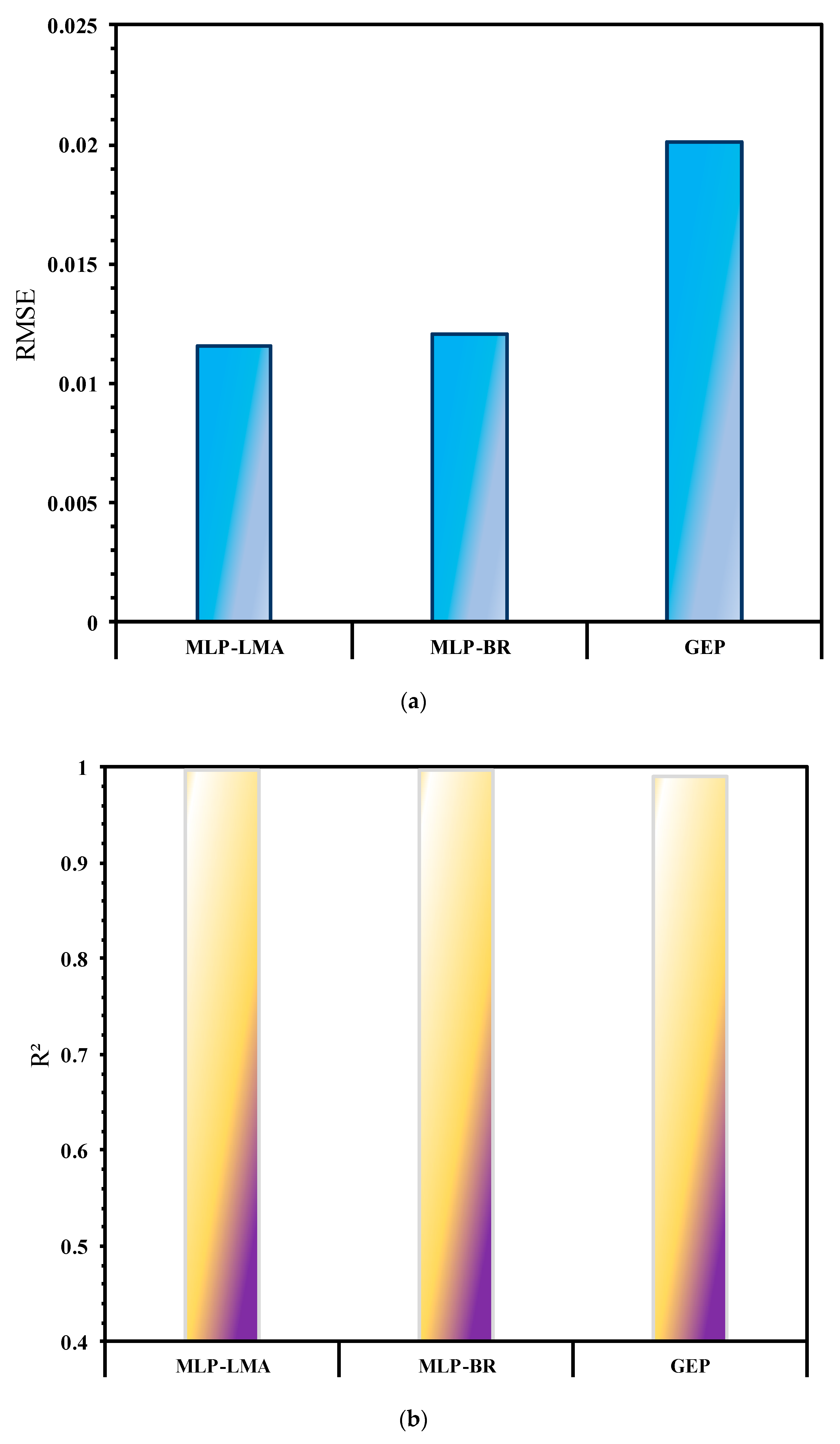
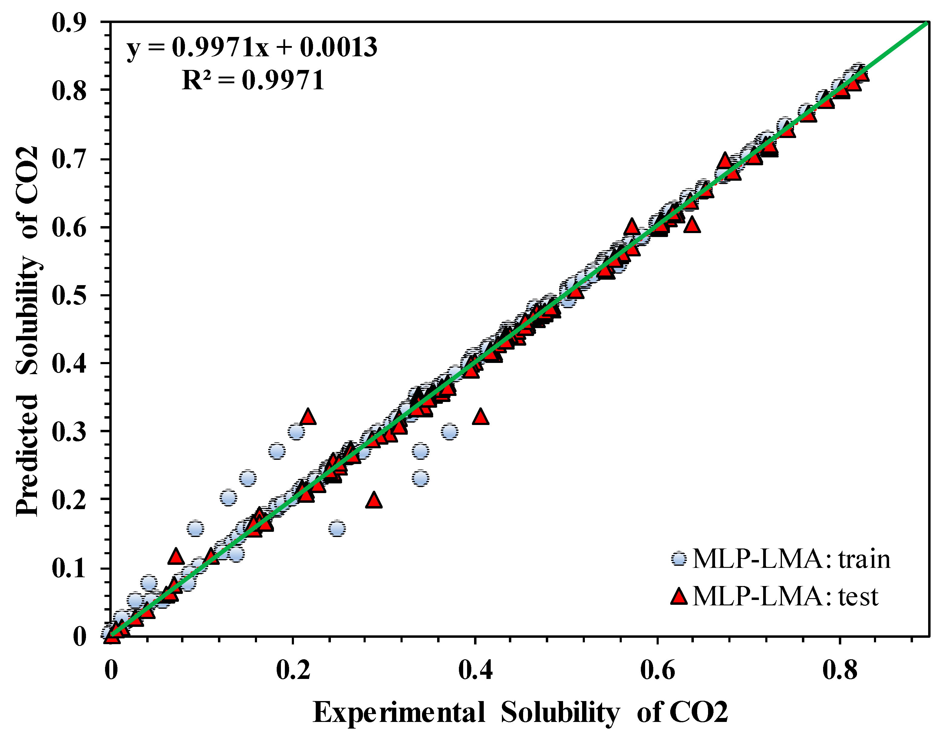
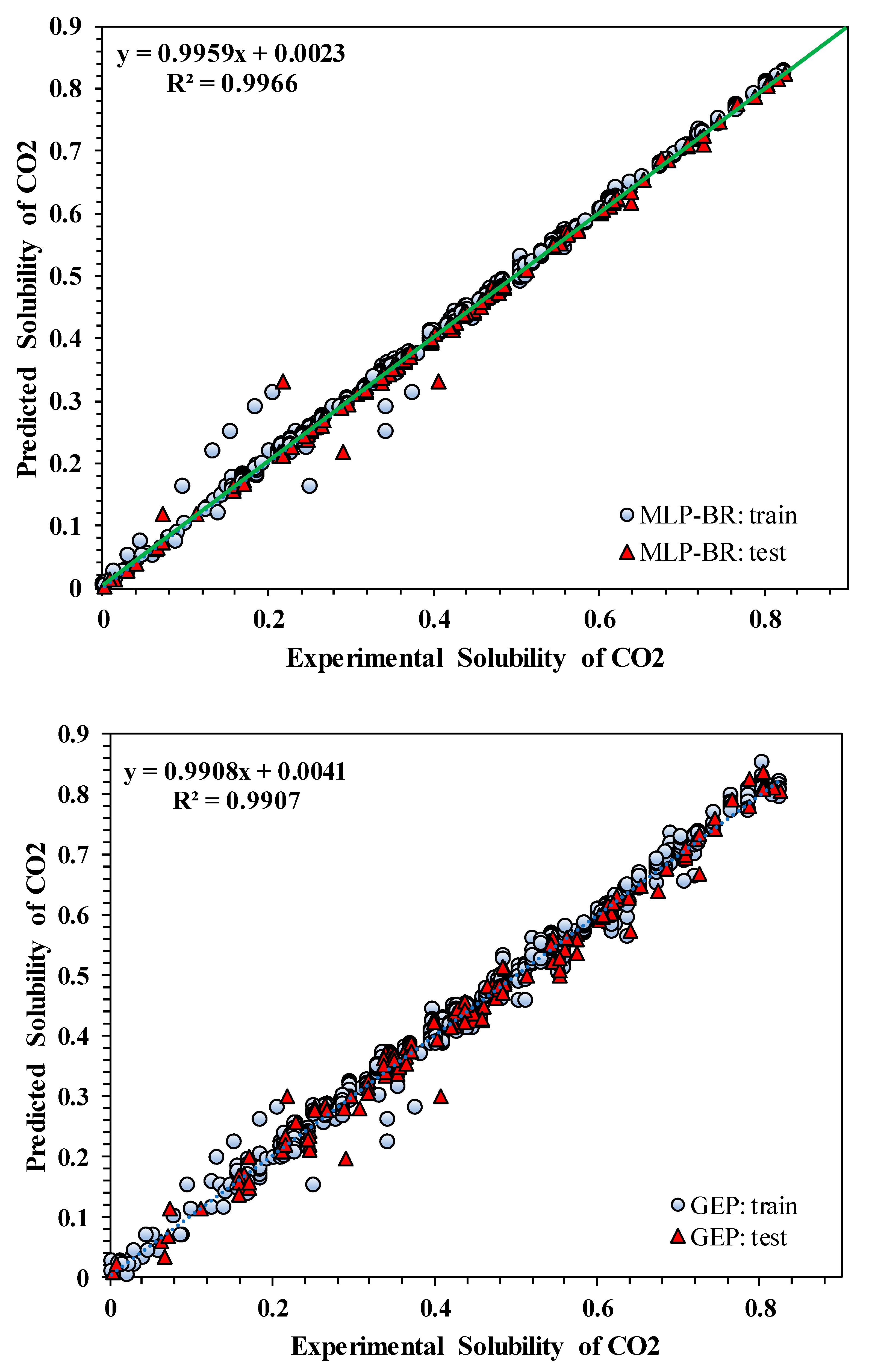
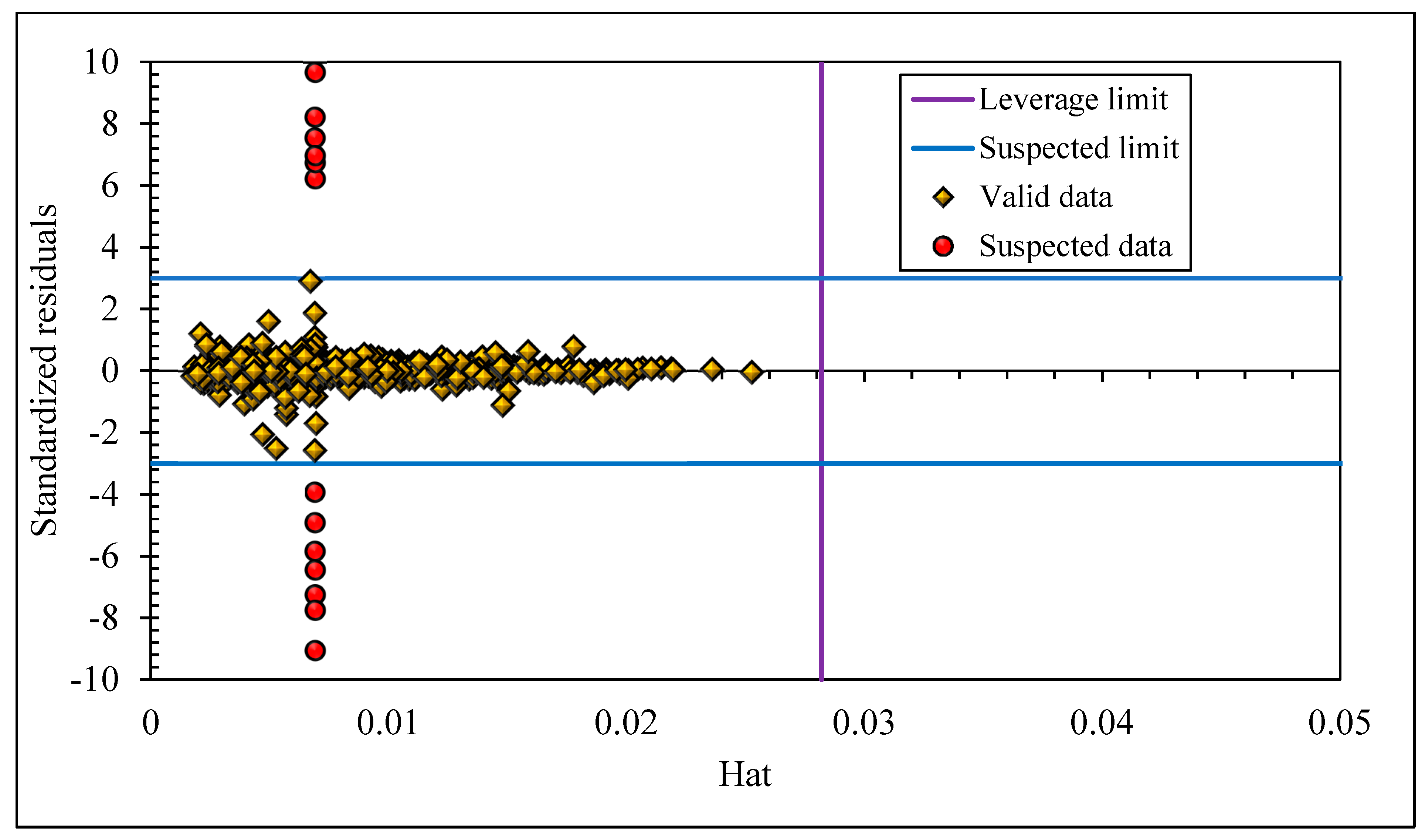
The current work aims at developing highly robust and easy-to-use machine learning models that can be applied for forecasting the solubility of CO2 in 13 different ionic liquids at different temperature and pressure conditions. Two rigorous connectionist techniques, namely multilayer perceptron (MLP), and gene expression programming (GEP) are applied on a set of experimental data that was gathered from different literature sources [40,41,42,43,44]. The MLP method was optimized using either Levenberg–Marquardt (LMA) or Bayesian Regularization (BR) techniques. The results obtained using three methods (MLP-LMA, MLP-BR, GEP) are then compared with results calculated using thermodynamic models based on Peng–Robinson (PR) and Soave–Redlich–Kwong (SRK) equation of states. Statistical indicators, including the determination coefficient (R2) and Root Mean Square Error (RMSE), are used to evaluate the accuracy of the methods, in addition to graphical assessments using cross plots and bar plots. In the end, outliers detection is performed to test and analyze the validity of the best-developed model and quantify the doubtful experimental points from the database. It is worth noting that the two backpropagation-based learning algorithms (LMA and BR) that were employed in the training process of MLP, alongside the explicit correlations established to predict the CO2 solubility in ILs, make the current work different from previously published works in the literature.
This paper is constructed as follows; Section 2 depicts the data used in the study and the input and output parameters in the models. Section 3 describes in detail the rigorous connectionist models and optimization techniques. An overview of the PR and SRK equations of state is presented in Section 4. In Section 5, the results are presented and discussed, and in Section 6, the conclusions of the study are summarized.

2. Data Collection and Preparation

In order to develop reliable models, it was crucial to use a large number of experimental data points representing a variety of conditions. In the current work, 744 experimental data points for carbon dioxide solubility in 13 different ILs (36 to 80 points for each IL) were collected from the literature [40,41,42,43,44]. Table 1 presents the references from where the data were gathered and the observed range of experimental measurements. The dissolved mole fraction (termed x ) of CO2 in each IL was the parameter we wished to match and predict based on the corresponding input of temperature T, pressure P, and the given IL. To represent the IL, we specified the thermodynamic properties of the IL, including molecular weight (Mw), critical temperature (Tc), critical pressure (Pc), and acentric factor (w), as summarized in Table 2. These 6 input parameters were hence used for predicting the dissolved mole fraction x of CO2. All the 744 experimental data points were randomly divided into a training data set (80% of the database) and a test data set (20% of the database).

3. Modeling Techniques

3.1. Multilayer Perceptron (MLP)

Artificial neural network (ANN) is one of the well-known machine learning tools, which exhibits reliable ability for recognizing and identifying relationships between input and output parameters in complex systems [45]. The conception and the mathematical formulation of an ANN model were inspired by the human brain and its strategy for processing information. Multilayer perceptron (MLP) is one of the most applied types of ANN for modeling purposes.
An MLP model includes three kinds of layers, an input layer: From which the inputs enter into the model. The i th input parameter of the model is noted z i .
One or more hidden layers: Their role is to transform the inputs into a higher feature in order to capture the non-linearity of the system. This mechanism is done by means of the activation functions. Tansig and logsig are among the frequently applied transfer functions and they are defined as follows:
Logsig :   g ( z ) = 1 e z + 1
Tansig :   g ( z ) = e z e z e z + e z
An output layer: The outputs of the model are returned from this layer. Pureline is generally considered the transfer function for this layer.
Pureline :   f ( z ) = z
If the total number of hidden layers is considered to be M , the input layer is defined as layer 0. Suppose that the number of neurons in the hidden layer m is N m , m = 1 ,   2 ,   ,   M . Considered w i j m the weight of the linkage between the j th neuron of the m 1 th hidden layer and i th neuron of the m th hidden layer, and b i m the bias term of ith neuron of the m th hidden layer. Hence, the output ( y ¯ i m ) of i th neuron of the m th hidden layer can be determined using the following equation:
y ¯ i m = f ( j = 1 N m 1 w i j m · y ¯ i m 1 + b i m )
y ¯ i 0 = z i ,   i = 1 ,   ,   N z ,   N z = N 0
Each of the above-mentioned layers includes neurons. The number of neurons in the input and output layers corresponds to the number of input and output parameters of the system, respectively. The number of hidden layers and their neurons depends on the complexity of the system. Generally, one hidden layer is sufficient to model systems having moderate complexity, while more than one hidden layer is recommended for highly complex systems. The trial and error method is usually applied for the proper determination of the number of hidden layers and their numbers of neurons.
The training phase of an MLP model consists of determining appropriate values for the weights and bias terms that result in the minimization of the difference between the experimental data (measured dissolved CO2 mole fraction) and the predictions of the model (calculated CO2 mole fraction as a function of the input parameters). Backpropagation learning techniques were applied for the training of the MLP model, namely the Bayesian Regularization (BR) and Levenberg–Marquardt (LM) algorithms. More details about these two algorithms can be found in prior published works [46,47,48].

3.2. Gene Expression Programming (GEP)

In spite of computer-based artificial intelligent models, based genetic calculations, such as genetic programming (GP) can construct formulas, which have high precision. It has been demonstrated that GP can be more accurate than traditional empirical models. Furthermore, models developed by genetic calculations and simulators and software systems are easy to use [49].
Using correction and development of the GP method [50] led to a more relevant version, which was GEP [51]. Indeed, the latter removed the found weaknesses in GP, i.e., the big number of possible programs that can be built by the algorithm and the high sensitivity to small changes in fitness of the created solution. In general, the GEP [51] had 2 significant parts: The chromosome and the symbolic expression trees (ETs). The chromosome encoded the potential solutions, and after that, these solutions were converted to the particular applicant solution named ET [52,53,54]. Reliable ETs continuously were reproduced by unlimited genetic conversions because of the conversion method of the structural organization of the chromosome to the ET [52]. In fact, the unique genes’ placements in the GEP method produced impressive development of the solutions leading to encryption of any downside [55]. Preceding researches recognized that the speed of convergence in the GEP scheme was much more than the GP scheme [53,54].
The chromosome included unchanging factors and variables as terminals and predetermined functions with equal length in one or more genes [52]. By the user, the constants were produced by the GEP in a specific range, however, the functions and variables were the input information. Each gene consisted of a tail, which comprised terminals and also a head that contained constants and variables in the role of terminals and functions [52]. The given value of the gene’s head is taken into account as an input of the GEP method, and the value of gene’s tail (t) is given by the following equation:
t = h(r − 1) + 1
with t denotes the length of the tail, h is the length of the head, and r is the number of arguments of the function with the most arguments.
The essential stages of the GEP method are illustrated in Figure 1. These steps can be elucidated briefly as follows: Firstly, a generation of chromosomes of an initial population was created randomly. In a second step, the chromosomes were expressed with ET, and their fitness was computed. Then, the individuals were selected to perform reproduction based on their fitness values. This reproduction created offspring with fresh signs. The same procedure was followed by individuals of the resulted generation, i.e., genomes expression, selection, and reproduction with adjustment. The stages expressed above were repeated until reaching the stopping criteria. More explanation of the GEP technique can be found in the literature [51,55].
In the current work, the mathematical expression used to predict the CO2 solubility in ILs was generated in the following form: x C O 2   =   f ( T ,   P ,   T c ,   I L ,   P c ,   I L   a n d   w I L ) .

3.3. Techniques Evaluation

Statistical indicators alongside the graphical techniques were used to assess the performance and robustness of the proposed models. The statistical indicators include root mean square error (RMSE) and the coefficient of determination (R2), which is defined mathematically as follows:
R M S E = 1 n i = 1 n ( x i   e x p x i   p r e d ) 2
R 2 = 1 i = 1 n ( x i   e x p x i   p r e d ) 2 i = 1 n ( x i   e x p x ¯ i   p r e d ) 2
The credibility of the developed models was tested using the leverage statistical approach. In this approach, the standardized residuals, which refer to the difference between the predicted results and the experimental points, were presented versus the statistical Hat matrix leverage values; this graph is called the Williams plot. The Hat can be calculated using the Hat matrix of the following form [56,57]:
H = X ( X t X ) 1 X t
where X is an (k × d) matrix, k and d represent the dimension and the data points number, respectively, and Xt denotes the X transpose matrix. The limit leverage value (H*) depicted on the Williams plot with a purple line is a constant calculated as 3(d + 1)/k. The selection of data points is in the range of ± 3 of the standard deviation from the mean, where the cut-off value of 3 ensures covering 99% of normally distributed data. The validity of the developed model and the credibility of the predictions were conditioned by the values of data points, which must be situated in the range of 0 ≤ H ≤ H* and −3 ≤ R ≤ 3.

4. Equations of State for Modeling the Solubility of Acid Gases

Many equations of state have been used by researchers to model the solubility of acid gases in ILs. Two of the most widely used EoS are the Soave–Redlich–Kwong (SRK) and the Peng–Robinson (PR) EoS, which are defined with Equations (10) and (15), respectively [35]. The results of these two EoS are used to contrast those obtained by using the proposed models.
Noting that the calculation of solubility using EoS is related to the calculation of the mole fraction, the equations below express how to determine the mole fraction.
Soave–Redlich–Kwong (SRK) EoS:
P = R T v b a ( T ) v ( v + b )
where T, P, v, and R indicate the temperature, pressure, molar volume, and gas constant respectively, and a and b represent the EoS variables.
For computing the variables, a and b in the case of mixtures, the classic van der Waals one-fluid rules of mixing is used [58]:
a = i = 1 N j = 1 N x i x j a i a j ( 1 K i j ( T ) ) ;   b = i = 1 N x i b i
with x i and x j denote the mole fractions of components i and j, and N indicates the number of the mixture’s components. The parameter K i j ( T ) is a parameter of binary interaction, that enlarges the molecular interactions between molecules i and j. For pure materials, the parameters can be computed as follows:
a i ( T ) = 0.42747 R 2 T c , i 2 P c , i α i ( T R )
b i = 0.08664 R T c , i P c , i
α i ( T R ) = [ 1 + ( 0.480 + 1.574 w i 0.176 w i 2 ) ( 1 T R i ) ] 2
with T R i = T T c i , denotes the reduced temperature. We note that the above description is valid for a system of arbitrarily many components. In our system, it was assumed that we had two components where CO2 was one and the IL the other.
Peng–Robinson (PR) EoS:
P = R T v b a ( T ) v ( v + b ) + b ( v b )
with:
a i ( T ) = 0.457235 R 2 T c , i 2 P c , i [ 1 + ( 0.37464 + 1.54226 w i 0.26992 w i 2 ) ( 1 T R i ) ] 2
b i = 0.077796 R T c , i P c , i
For mixtures, the parameters a and b are determined using the same formulas as in SRK EoS. The parameter of binary interaction ( K i j ) is the only adjustable parameter for both EoS, SRK, and PR. This parameter is determined using a genetic algorithm (GA) with the next objective function [58]:
f = i = 1 N ( x s o l u t e e x p x s o l u t e c a l x s o l u t e e x p ) 2
with x s o l u t e e x p and x s o l u t e c a l indicate the experimental and EoS-calculated mole fractions of the solute respectively.

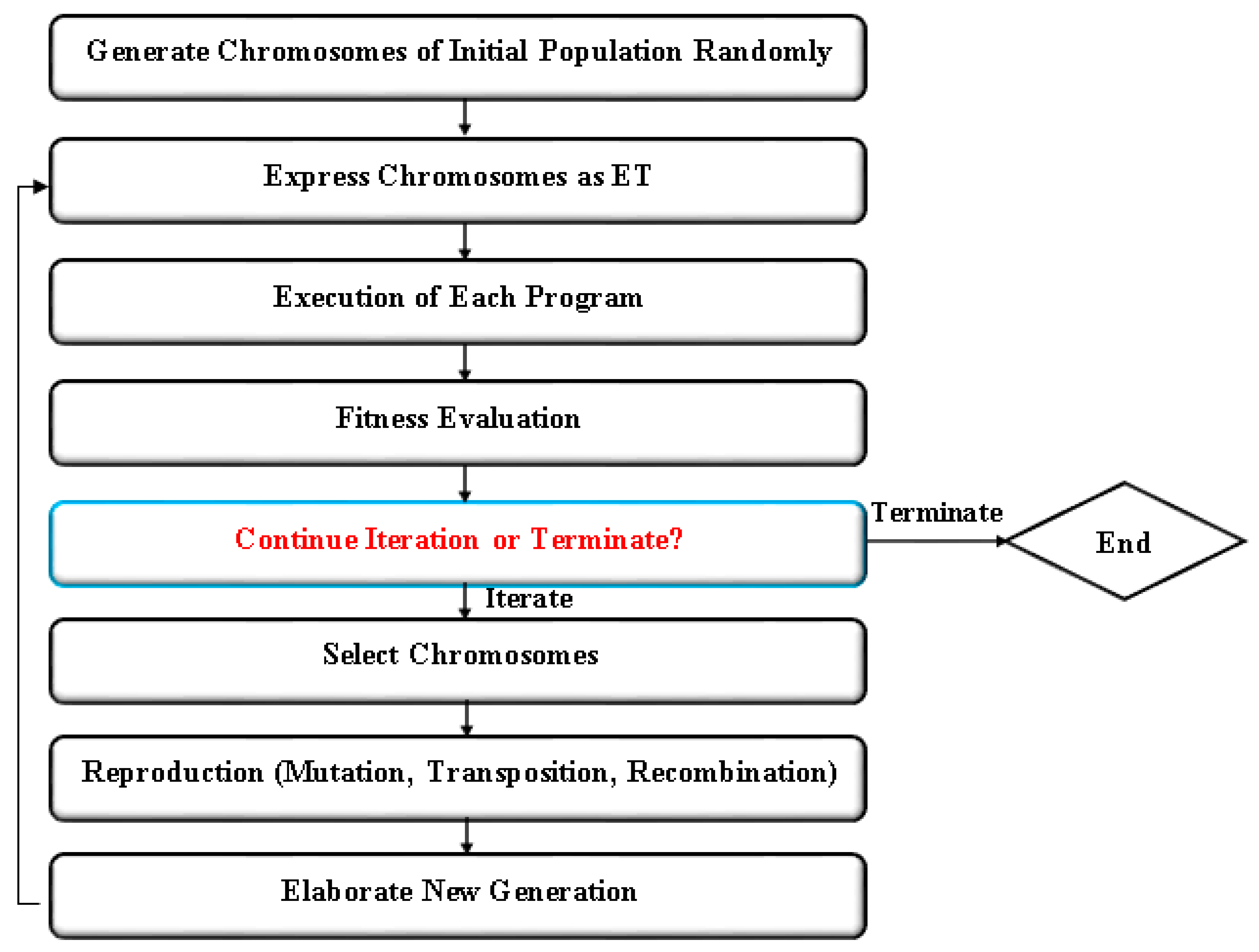
5. Computational Procedure

For the training phase, the mean square error (MSE) was used as the assessment criterion, which is defined mathematically as follows:
M S E = 1 n ( x i e x p x i p r e ) 2 n
where x stands for mole fraction of CO2, e x p and p r e d indicate the experimental and the predicted values, respectively, and n represents the number of samples. The model tuning parameters giving the lowest MSE on the training set were considered the choice for the trained model.
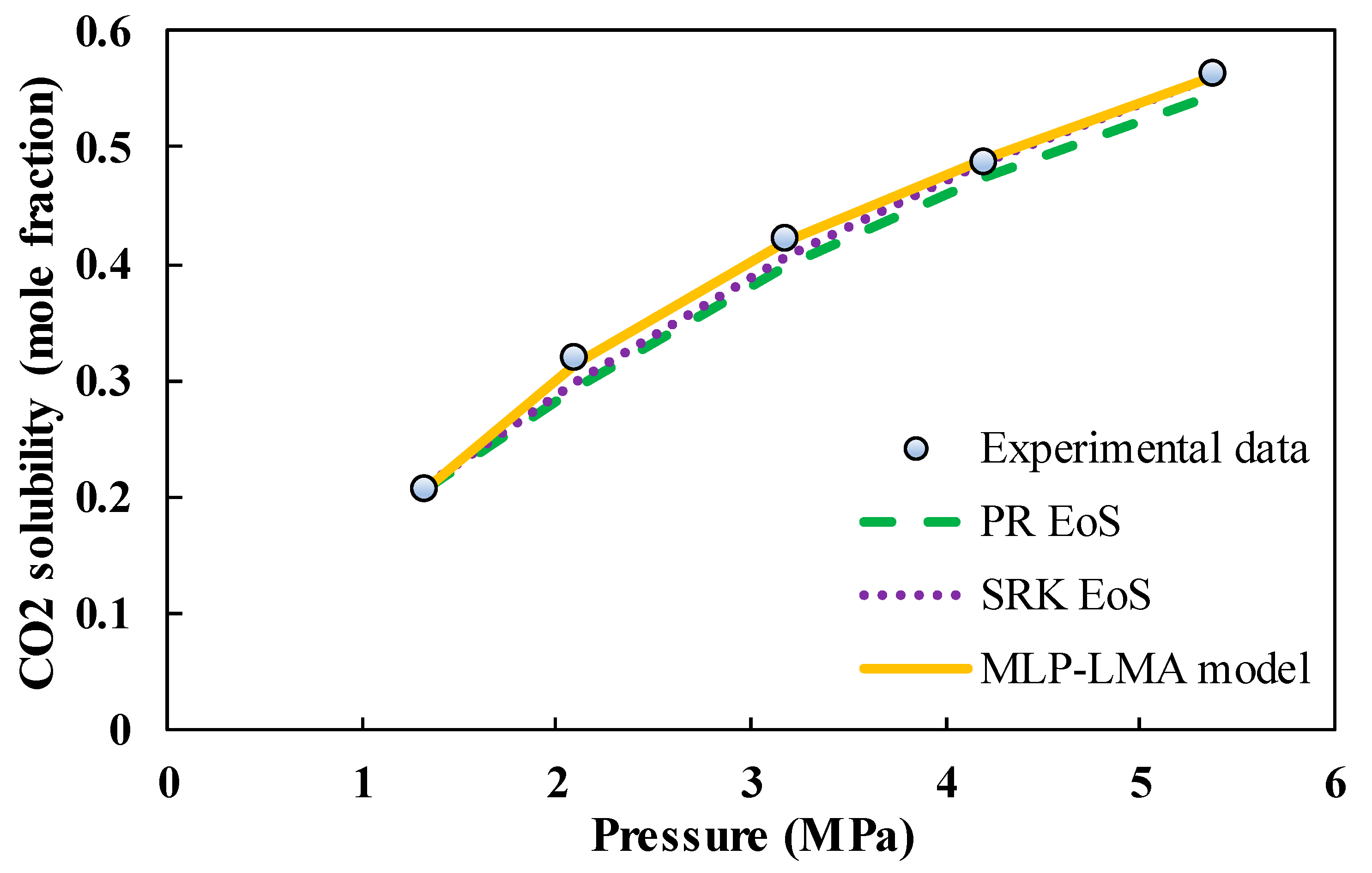
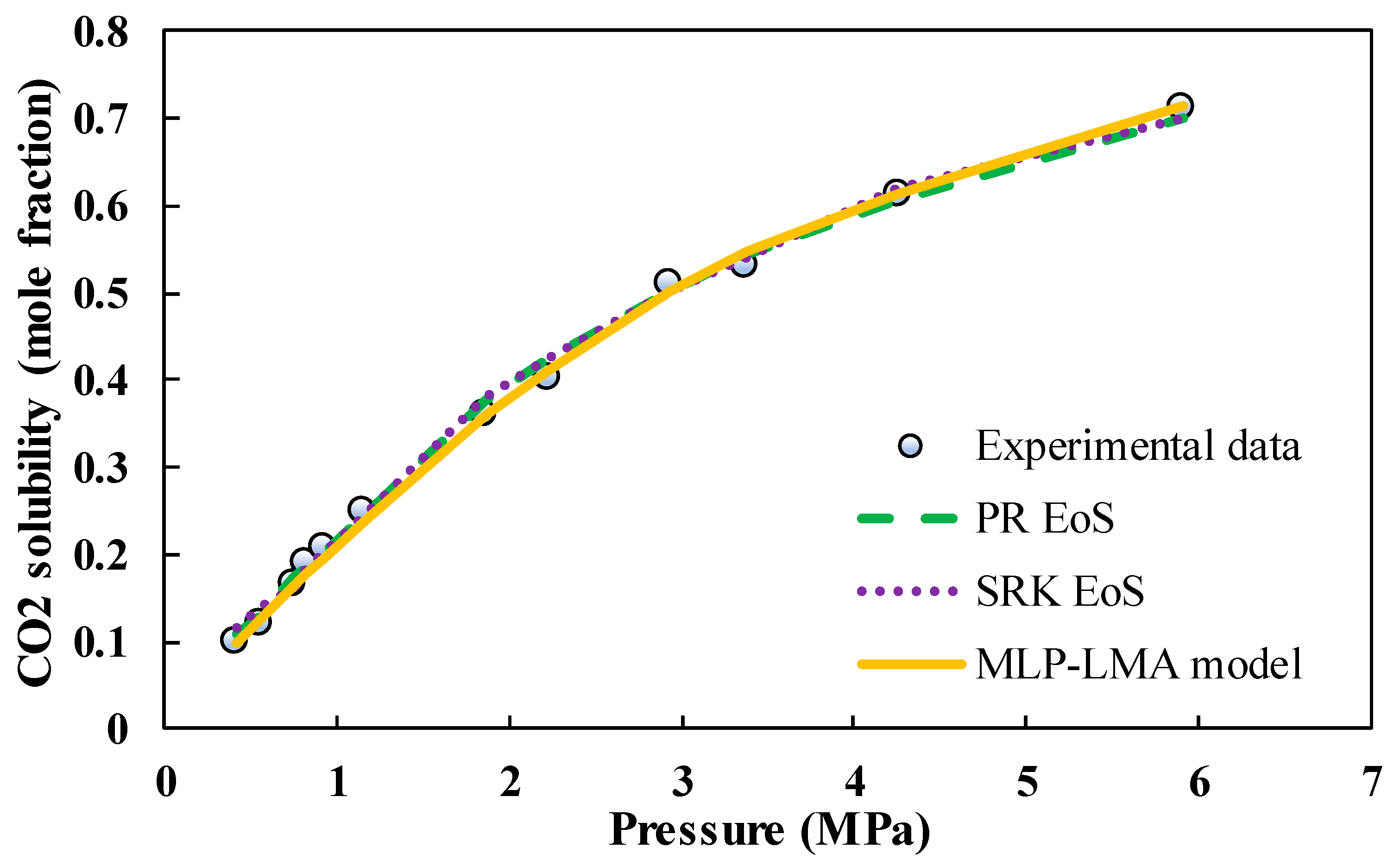
For the modeling task using MLP, the data points were normalized between −1 and 1. To select appropriate topologies for the MLP approach, trial and error were used. The obtained models were designated MLP-LMA, and MLP-BR, respectively, and both included 3 hidden layers with 11, 11, and 9 neurons, respectively. The suitable activation functions in all the hidden layers and for the output layer were Tansig and Pureline, respectively.

6. Results and Discussion

To obtain an accurate and trustworthy expression, the calculation procedure reported in Section 3.2 has been followed. Thus, taking into account the series of five independent parameters ( T ,   P ,   T c ,   P c ,   w ) , the GEP-based model makes the mathematical based correlation for the dependent parameter x C O 2 as follows:
x = 0.0001011 × A 1 + A 2 tanh ( P ) A 3 P + A 4 × ln ( P ) + 10 6 × M w 2 × A 5 + A 6 × P c 3 + A 7 × T c + A 8
where P (MPa) and P c (MPa) are pressure and critical pressure, respectively, M w (Kg/Kmole) is the molecular weight, T c (K) indicates the critical temperature and A 1 , A 2 , A 3 …… and A 8 are expressed as below:
A 1 = P c × w + P × ( P c + w + P )
A 2 = 3.362 0.1832 × T
A 3 = 0.4802 + 0.08072 × T M w + 0.03085 × T + 5.14 × 10 6 × M w × P × ln ( T )
A 4 = 0.3091 tanh ( P c ) 0.4344 P c 3 0.002638 × exp ( P c )
A 5 = 4.047 5.481 × 10 3 × M w
A 6 = 2.33 × 10 5 × T c × tanh ( M w ) 0.0004489 × P c 3
A 7 = 4.047 × 10 6 0.000305 × w A 8 = 5.213 × 10 7 × P 3 0.146 × P c + 0.5632 × w + 0.04124 × exp ( T M w ) 0.2381 × ln ( tanh ( P ) ) 0.339

6.1. Performance Evaluation

Table 3 summarizes the statistical parameters (RMSE and R2) of the three proposed models in predicting CO2 solubility for training, test, and overall data. The graphical representation of the overall RMSE and R2 through bar plots, as shown in Figure 2. This graphical comparison allows an alternative visualization for the performance of the different models. A concise view of the figure shows that the values of RMSE and R2 were closest to 0 and 1, respectively, pointing out that the models were more credible and qualified for the forecast.
Form a deep comparative standing point of view, Table 3 and Figure 2 show that the reliability of the developed models took the following order: MLP-LMA > MLP-BR > GEP. The MLP model optimized using LMA had the highest R2 coefficients and the lowest RMSE values for both the training and overall data, followed by the MLP-BR model. On the other hand, very satisfactory performances and high predictions potential of the GEP model were asserted by the values reported in Table 3 for training, test, and overall data.
Cross plots in Figure 3 were used to compare the models’ predictions against the experimental data further. In these plots, the predicted values using the three methods were represented versus the previously established experimental data for the solubility of CO2 in ILs. The criterion of precision for the different models in typical cross plots can be indicated by the compressed gathering of data points cloud nearby the 45° line, otherwise, all points falling on the unit slope would correspond to a perfect model. The accumulation of data cloud nearby the 45° line was attributed to the elevated value of R2 close to the unit and to the low value of RMSE near zero.
It can be observed in Figure 3, that the MLP-LMA, MLP-BR, and GEP models exhibited distributions of predictions near the unit slope line for both training and test datasets, confirming their high accuracy in estimating the solubility of CO2 in the considered ionic liquids.

6.2. Comparison with PR and SRK EoS Results

The results obtained by the MLP-LMA model were compared with values calculated using thermodynamic models based on PR and SRK EoS.
Table 4 and Table 5 provide the CO2 solubility and thermodynamic properties respectively. Furthermore, Table 6 summarizes a comparison, where the RMSEs and R2 of the best-proposed model, i.e., MLP-LMA, and PR and SRK EoS were mentioned. To perform this comparison, two samples of ILs that had not been included in the training phase of the intelligent models were considered. These samples included [bmim][Tf2N] and [bmim][PF6] ILs. Further description is given in Table 4 and Table 5. All three models (MLP-LMA, and the PR and SRK EoS) gave accurate descriptions with R 2 above 0.98. For the two ILs, the MLP-LMA model had a higher coefficient of determination and lower RMSE compared to the PR and SRK EoS, in the following order of reliability: MLP-LMA > SRK > PR in the case of [bmim][PF6], and MLP-LMA > PR > SRK in the case of [bmim][Tf2N].
Figure 4 and Figure 5 exhibited the comparison performed between PR and SRK EoS and the MLP-LMA model, and at the same time, the evolution of CO2 solubility with pressure in the two ILs at a constant temperature. As it is clear in the figures, the solubility of CO2 increased with the increase in pressure for the two investigated ILs. Henry’s law can explain this phenomenon, which supposes that the gas solubility throughout a liquid is directly a function of the gas pressure above the solution’s surface [28]. The increase in pressure forces gas molecules into the solution, thus the number of gas molecules dissolved raises. It can also be seen from the figures that the solubility values predicted by the MLP-LMA model are in good agreement with the experimental data, whereas those established using the EoS differs slightly.

6.3. Outlier Detection

A Williams plot of the MLP-LMA model is depicted in Figure 6. It can be seen from the figure that the majority of data points are situated in the range of −3 ≤ R ≤ 3 and 0 ≤ H ≤ 0.03, which validated and verified the implemented MLP-LMA model statistically, where 13 points are considered suspect. In summary, the leverage approach states that the developed model is reliable and can be used with high accuracy to predict CO2 solubility in ILs.

7. Conclusions

In the current paper, based on different experimental data gathered from the literature, MLP-LMA, GEP, PR, and SRK EoS methods were successfully used to predict carbon dioxide solubility in 13 various ionic liquids under the (298.15–373.15 K) temperature and (0.01–100.12 MPa) pressure range. Multilayer perceptron optimized with two back-propagation algorithms, viz. LMA and BR, and a reliable white-box technique, namely GEP, were the applied data-driven methods. The various statistical indicators obtained in this study showed that MLP optimized with LMA was the most advantageous paradigm, which can be used with high precision to predict the CO2 solubility in ILs for natural gas sweetening and purification process, which may be of great interest for experts and gas engineers. Furthermore, the established correlation using the GEP-based model was reliable and gave good results. Finally, the comparison made between the MLP-LMA model and PR and SRK EoS demonstrated the high performance of the proposed model against the cubic EoS.

Author Contributions

Data curation, H.O., N.N., and A.M.; formal analysis, H.O., P.Ø.A., and A.M.; funding acquisition, A.M.; investigation, A.H.H., M.E.A.B.S., P.Ø.A., and S.S.; methodology, A.H.H. and M.E.A.B.S.; project administration, M.N.A., M.A.G., and N.N.; resources, M.N.A., M.A.G., and N.N.; software, M.N.A., M.A.G., and N.N.; supervision, S.S.; writing—original draft, H.O.; writing—review and editing, P.Ø.A. and A.M. All authors have read and agreed to the published version of the manuscript.

Funding

We acknowledge the financial support of this work by the Hungarian State and the European Union under the EFOP-3.6.1-16-2016-00010 project.

Acknowledgments

We acknowledge the support of the German Research Foundation (DFG) and the Bauhaus-Universität Weimar within the Open-Access Publishing Programme. Furthermore, we acknowledge the Research Council of Norway and the industry partners, ConocoPhillips Skandinavia AS, Aker BP ASA, Vår Energi AS, Equinor ASA, Neptune Energy Norge AS, Lundin Norway AS, Halliburton AS, Schlumberger Norge AS, and Wintershall DEA, of The National IOR Centre of Norway for support.

Conflicts of Interest

The authors declare no conflict of interest.

Abbreviations and Symbols

ANNArtificial neural network
BRBayesian Regularization
CO2Carbon dioxide
dData points number
DEADiethanolamine
EoSEquations of state
ETsExpression trees
e x p Experimental
FLFuzzy logic
GEPGene expression programming
GPGenetic programming
H Hat matrix
H2SHydrogen sulfide
H*Limit Leverage value
ILsIonic liquids
LMLevenberg–Marquardt
MEAMonoethanolamine
MLPMultilayer perceptron
MSEMean square error
MwMolecular weight (kg/kmole)
kDimension
n Number of samples
PcCritical pressure (MPa)
p r e d Predicted
PRPeng–Robinson
RMSERoot mean square error
R2Coefficient of determination
SRKSoave–Redlich–Kwong
SVMSupport vector machine
tGene’s tail
TcCritical temperature (K)
TEATriethanolamine
wAcentric factor
x Mole fraction of CO2
X(k × d) matrix
XtX transpose matrix

References

  1. Taib, M.M.; Murugesan, T. Solubilities of CO2 in aqueous solutions of ionic liquids (ILs) and monoethanolamine (MEA) at pressures from 100 to 1600 kPa. Chem. Eng. J. 2012, 181, 56–62. [Google Scholar] [CrossRef]
  2. Kidnay, A.J.; Parrish, W.R.; McCartney, D.G. Fundamentals of Natural Gas Processing; CRC Press: Boca Raton, FL, USA, 2011. [Google Scholar]
  3. Astaria, G.; Savage, D.W.; Bisio, A. Gas Treating with Chemical Solvents; John Wiley: New York, NY, USA, 1983. [Google Scholar]
  4. Romeo, L.M.; Bolea, I.; Escosa, J.M. Integration of power plant and amine scrubbing to reduce CO2 capture costs. Appl. Therm. Eng. 2008, 28, 1039–1046. [Google Scholar] [CrossRef]
  5. Mulukutla, T.; Obuskovic, G.; Sirkar, K.K. Novel scrubbing system for post-combustion CO2 capture and recovery: Experimental studies. J. Membr. Sci. 2014, 471, 16–26. [Google Scholar] [CrossRef]
  6. Jalili, A.H.; Rahmati-Rostami, M.; Ghotbi, C.; Hosseini-Jenab, M.; Ahmadi, A.N. Solubility of H2S in ionic liquids [bmim][PF6], [bmim][BF4], and [bmim][Tf2N]. J. Chem. Eng. Data 2009, 54, 1844–1849. [Google Scholar] [CrossRef]
  7. Shiflett, M.B.; Yokozeki, A. Separation of CO2 and H2S using room-temperature ionic liquid [bmim][PF6]. Fluid Phase Equilib. 2010, 294, 105–113. [Google Scholar] [CrossRef]
  8. Sakhaeinia, H.; Taghikhani, V.; Jalili, A.H.; Mehdizadeh, A.; Safekordi, A.A. Solubility of H2S in 1-(2-hydroxyethyl)-3-methylimidazolium ionic liquids with different anions. Fluid Phase Equilib. 2010, 298, 303–309. [Google Scholar] [CrossRef]
  9. Sánchez, L.G.; Meindersma, G.; De Haan, A. Solvent properties of functionalized ionic liquids for CO2 absorption. Chem. Eng. Res. Des. 2007, 85, 31–39. [Google Scholar] [CrossRef] [Green Version]
  10. Safavi, M.; Ghotbi, C.; Taghikhani, V.; Jalili, A.H.; Mehdizadeh, A. Study of the solubility of CO2, H2S and their mixture in the ionic liquid 1-octyl-3-methylimidazolium hexafluorophosphate: Experimental and modelling. J. Chem. Thermodyn. 2013, 65, 220–232. [Google Scholar] [CrossRef]
  11. Han, D.; Tian, M.; Park, D.-W.; Choi, D.K. Application of ionic liquids as mobile phase additives and surface-bonded stationary phase in liquid chromatography. Korean J. Chem. Eng. 2009, 26, 1353–1358. [Google Scholar] [CrossRef]
  12. Martínez-Paloua, R.; Luqueb, R. Applications of Ionic liquids in contaminants removal from Refinery Feedstocks: An industrial perspective. Energy Environ. Sci. 2014, 7, 2414–2447. [Google Scholar] [CrossRef]
  13. Bemani, A.; Baghban, A.; Shamshirband, S.; Mosavi, A.; Csiba, P.; Varkonyi-Koczy, A.R. Applying ANN, ANFIS, and LSSVM Models for Estimation of Acid Solvent Solubility in Supercritical CO2. arXiv 2019, arXiv:1912.05612. [Google Scholar] [CrossRef]
  14. Shamshirband, S.; Hadipoor, M.; Baghban, A.; Mosavi, A.; Bukor, J.; Várkonyi-Kóczy, A.R. Developing an ANFIS-PSO Model to Predict Mercury Emissions in Combustion Flue Gases. Mathematics 2019, 7, 965. [Google Scholar]
  15. Hasib-ur-Rahman, M.; Siaj, M.; Larachi, F. Ionic liquids for CO2 capture—Development and progress. Chem. Eng. Process. 2010, 49, 313–322. [Google Scholar] [CrossRef]
  16. Bara, J.E. Potential for hydrogen sulfide removal using ionic liquid solvents. In Green Solvents II; Springer: Berlin/Heidelberg, Germany, 2012; pp. 155–167. [Google Scholar]
  17. Davis, H.; James, J. Task-specific ionic liquids. Chem. Lett. 2004, 33, 1072–1077. [Google Scholar] [CrossRef]
  18. Akhmetshina, A.I.; Petukhov, A.N.; Gumerova, O.R.; Vorotyntsev, A.V.; Nyuchev, A.V.; Vorotyntsev, I.V. Solubility of H2S and CO2 in imidazolium-based ionic liquids with bis (2-ethylhexyl) sulfosuccinate anion. J. Chem. Thermodyn. 2019, 130, 173–182. [Google Scholar] [CrossRef]
  19. Jalili, A.H.; Mehrabi, M.; Zoghi, A.T.; Shokouhi, M.; Taheri, S.A. Solubility of carbon dioxide and hydrogen sulfide in the ionic liquid 1-butyl-3-methylimidazolium trifluoromethanesulfonate. Fluid Phase Equilib. 2017, 453, 1–12. [Google Scholar] [CrossRef]
  20. Yokozeki, A.; Shiflett, M.B.; Junk, C.P.; Grieco, L.M.; Foo, T. Physical and chemical absorptions of carbon dioxide in room-temperature ionic liquids. J. Phys. Chem. B 2008, 112, 16654–16663. [Google Scholar] [CrossRef]
  21. Kurnia, K.; Harris, F.; Wilfred, C.; Mutalib, M.A.; Murugesan, T. Thermodynamic properties of CO2 absorption in hydroxyl ammonium ionic liquids at pressures of (100–1600) kPa. J. Chem. Thermodyn. 2009, 41, 1069–1073. [Google Scholar] [CrossRef]
  22. Carvalho, P.J.; Álvarez, V.H.; Schröder, B.; Gil, A.M.; Marrucho, I.M.; Aznar, M.; Santos, L.M.; Coutinho, J.A. Specific solvation interactions of CO2 on acetate and trifluoroacetate imidazolium based ionic liquids at high pressures. J. Phys. Chem. B 2009, 113, 6803–6812. [Google Scholar] [CrossRef]
  23. Shin, E.-K.; Lee, B.-C. High-pressure phase behavior of carbon dioxide with ionic liquids: 1-alkyl-3-methylimidazolium trifluoromethanesulfonate. J. Chem. Eng. Data 2008, 53, 2728–2734. [Google Scholar] [CrossRef]
  24. Yuan, X.; Zhang, S.; Liu, J.; Lu, X. Solubilities of CO2 in hydroxyl ammonium ionic liquids at elevated pressures. Fluid Phase Equilib. 2007, 257, 195–200. [Google Scholar] [CrossRef]
  25. Vega, L.F.; Vilaseca, O.; Llovell, F.; Andreu, J.S. Modeling ionic liquids and the solubility of gases in them: Recent advances and perspectives. Fluid Phase Equilib. 2010, 294, 15–30. [Google Scholar] [CrossRef]
  26. Rahmati-Rostami, M.; Ghotbi, C.; Hosseini-Jenab, M.; Ahmadi, A.N.; Jalili, A.H. Solubility of H2S in ionic liquids [hmim][PF6], [hmim][BF4], and [hmim][Tf2N]. J. Chem. Thermodyn. 2009, 41, 1052–1055. [Google Scholar] [CrossRef]
  27. Shokouhi, M.; Adibi, M.; Jalili, A.H.; Hosseini-Jenab, M.; Mehdizadeh, A. Solubility and diffusion of H2S and CO2 in the ionic liquid 1-(2-hydroxyethyl)-3-methylimidazolium tetrafluoroborate. J. Chem. Eng. Data 2009, 55, 1663–1668. [Google Scholar] [CrossRef]
  28. Jalili, A.H.; Mehdizadeh, A.; Shokouhi, M.; Ahmadi, A.N.; Hosseini-Jenab, M.; Fateminassab, F. Solubility and diffusion of CO2 and H2S in the ionic liquid 1-ethyl-3-methylimidazolium ethylsulfate. J. Chem. Thermodyn. 2010, 42, 1298–1303. [Google Scholar] [CrossRef]
  29. Jou, F.-Y.; Mather, A.E. Solubility of hydrogen sulfide in [bmim][PF 6]. Int. J. Thermophys. 2007, 28, 490. [Google Scholar] [CrossRef]
  30. Yokozeki, A.; Shiflett, M.B. Gas solubilities in ionic liquids using a generic van der Waals equation of state. J. Supercrit. Fluids 2010, 55, 846–851. [Google Scholar] [CrossRef]
  31. Zhang, S.; Chen, Y.; Ren, R.X.-F.; Zhang, Y.; Zhang, J.; Zhang, X. Solubility of CO2 in sulfonate ionic liquids at high pressure. J. Chem. Eng. Data 2005, 50, 230–233. [Google Scholar] [CrossRef]
  32. Kim, Y.; Jang, J.; Lim, B.; Kang, J.W.; Lee, C. Solubility of mixed gases containing carbon dioxide in ionic liquids: Measurements and predictions. Fluid Phase Equilib. 2007, 256, 70–74. [Google Scholar] [CrossRef]
  33. Al-fnaish, H.; Lue, L. Modelling the solubility of H2S and CO2 in ionic liquids using PC-SAFT equation of state. Fluid Phase Equilib. 2017, 450, 30–41. [Google Scholar] [CrossRef] [Green Version]
  34. Cybenko, G. Approximation by superpositions of a sigmoidal function. Math. Control Signals Syst. 1989, 2, 303–314. [Google Scholar] [CrossRef]
  35. Ahmadi, M.A.; Ebadi, M.; Hosseini, S.M. Prediction breakthrough time of water coning in the fractured reservoirs by implementing low parameter support vector machine approach. Fuel 2014, 117, 579–589. [Google Scholar] [CrossRef]
  36. Baghban, A.; Ahmadi, M.A.; Shahraki, B.H. Prediction carbon dioxide solubility in presence of various ionic liquids using computational intelligence approaches. J. Supercrit. Fluids 2015, 98, 50–64. [Google Scholar] [CrossRef]
  37. Vapnik, V.; Vapnik, V. Statistical Learning Theory; Wiley: New York, NY, USA, 1998. [Google Scholar]
  38. Amedi, H.R.; Baghban, A.; Ahmadi, M.A. Evolving machine learning models to predict hydrogen sulfide solubility in the presence of various ionic liquids. J. Mol. Liquids 2016, 216, 411–422. [Google Scholar] [CrossRef]
  39. Rostami, A.; Arabloo, M.; Kamari, A.; Mohammadi, A.H. Modeling of CO2 solubility in crude oil during carbon dioxide enhanced oil recovery using gene expression programming. Fuel 2017, 210, 768–782. [Google Scholar] [CrossRef]
  40. Kim, S.A.; Yim, J.-H.; Lim, J.S. High-pressure phase behavior of binary mixtures containing methylpyrrolidinium derivative ionic liquids and carbon dioxide. Fluid Phase Equilib. 2012, 332, 28–34. [Google Scholar] [CrossRef]
  41. Tagiuri, A.; Sumon, K.Z.; Henni, A. Solubility of carbon dioxide in three [Tf2N] ionic liquids. Fluid Phase Equilib. 2014, 380, 39–47. [Google Scholar] [CrossRef]
  42. Yim, J.-H.; Lim, J.S. CO2 solubility measurement in 1-hexyl-3-methylimidazolium ([HMIM]) cation based ionic liquids. Fluid Phase Equilib. 2013, 352, 67–74. [Google Scholar] [CrossRef]
  43. Kim, J.E.; Kim, H.J.; Lim, J.S. Solubility of CO2 in ionic liquids containing cyanide anions: [c2mim][SCN], [c2mim][N(CN)2], [C2mim][C(CN)3]. Fluid Phase Equilib. 2014, 367, 151–158. [Google Scholar] [CrossRef]
  44. Yim, J.-H.; Song, H.N.; Yoo, K.-P.; Lim, J.S. Measurement of CO2 solubility in ionic liquids: [BMP][Tf2N] and [BMP][MeSO4] by measuring bubble-point pressure. J. Chem. Eng. Data 2011, 56, 1197–1203. [Google Scholar] [CrossRef]
  45. Hemmati-Sarapardeh, A.; Ameli, F.; Varamesh, A.; Shamshirband, S.; Mohammadi, A.H.; Dabir, B. Toward generalized models for estimating molecular weights and acentric factors of pure chemical compounds. Int. J. hydrog. Energy 2018, 43, 2699–2717. [Google Scholar] [CrossRef]
  46. Hemmati-Sarapardeh, A.; Varamesh, A.; Husein, M.M.; Karan, K. On the evaluation of the viscosity of nanofluid systems: Modeling and data assessment. Renew. Sustain. Energy Rev. 2018, 81, 313–329. [Google Scholar] [CrossRef]
  47. Menad, N.A.; Hemmati-Sarapardeh, A.; Varamesh, A.; Shamshirband, S. Predicting solubility of CO2 in brine by advanced machine learning systems: Application to carbon capture and sequestration. J. CO2 Util. 2019, 33, 83–95. [Google Scholar] [CrossRef]
  48. Menad, N.A.; Noureddine, Z.; Hemmati-Sarapardeh, A.; Shamshirband, S. Modeling temperature-based oil-water relative permeability by integrating advanced intelligent models with grey wolf optimization: Application to thermal enhanced oil recovery processes. Fuel 2019, 242, 649–663. [Google Scholar] [CrossRef]
  49. Fathinasab, M.; Ayatollahi, S.; Hemmati-Sarapardeh, A. A rigorous approach to predict nitrogen-crude oil minimum miscibility pressure of pure and nitrogen mixtures. Fluid Phase Equilib. 2015, 399, 30–39. [Google Scholar] [CrossRef]
  50. Koza, J.R.; Koza, J.R. Genetic Programming: On the Programming of Computers by Means of Natural Selection; MIT Press: Cambridge, MA, USA, 1992; Volume 1. [Google Scholar]
  51. Ferreira, C. Gene expression programming: A new adaptive algorithm for solving problems. Complex Syst. 2019, 3, 183–199. [Google Scholar]
  52. Teodorescu, L.; Sherwood, D. High energy physics event selection with gene expression programming. Comput. Phys. Commun. 2008, 178, 409–419. [Google Scholar] [CrossRef]
  53. Rostami, A.; Ebadi, H. Toward gene expression programming for accurate prognostication of the critical oil flow rate through the choke: Correlation development. Asia-Pac. J. Chem. Eng. 2017, 12, 884–893. [Google Scholar] [CrossRef]
  54. Rostami, A.; Shokrollahi, A. Accurate prediction of water dewpoint temperature in natural gas dehydrators using gene expression programming approach. J. Mol. Liquids 2017, 243, 196–204. [Google Scholar] [CrossRef]
  55. Ferreira, C. Gene Expression Programming: Mathematical Modeling by an Artificial Intelligence; Springer: Berlin/Heidelberg, Germany, 2006; Volume 21. [Google Scholar]
  56. Kamari, A.; Safiri, A.; Mohammadi, A.H. Compositional model for estimating asphaltene precipitation conditions in live reservoir oil systems. J. Dispers. Sci. Technol. 2015, 36, 301–309. [Google Scholar] [CrossRef]
  57. Jaworska, J.; Nikolova-Jeliazkova, N.; Aldenberg, T. QSAR applicability domain estimation by projection of the training set in descriptor space: A review. Altern. Lab. Anim. 2005, 33, 445–459. [Google Scholar] [CrossRef]
  58. Haghbakhsh, R.; Soleymani, H.; Raeissi, S. A simple correlation to predict high pressure solubility of carbon dioxide in 27 commonly used ionic liquids. J. Supercrit. Fluids 2013, 77, 158–166. [Google Scholar] [CrossRef]
  59. Aki, S.N.; Mellein, B.R.; Saurer, E.M.; Brennecke, J.F. High-pressure phase behavior of carbon dioxide with imidazolium-based ionic liquids. J. Phys. Chem. B 2004, 108, 20355–20365. [Google Scholar] [CrossRef]
  60. Anthony, J.L.; Anderson, J.L.; Maginn, E.J.; Brennecke, J.F. Anion effects on gas solubility in ionic liquids. J. Phys. Chem. B 2005, 109, 6366–6374. [Google Scholar] [CrossRef] [PubMed] [Green Version]
Figure 1. Flowchart of gene expression programming (GEP) algorithm procedure.
Applsci 10 00304 g001
Figure 2. Performance comparison on the overall dataset for the proposed models: (a) Root mean square error (RMSE), and (b) R2.
Applsci 10 00304 g002
Figure 3. Cross plots of the proposed predictive models.
Applsci 10 00304 g003aApplsci 10 00304 g003b
Figure 4. Comparison of Peng–Robinson (PR) and Soave–Redlich–Kwong equations of state (SRK EoS), and MLP-LMA model for prediction of CO2 solubility in [bmim][PF6] at T = 298.15 K.
Applsci 10 00304 g004
Figure 5. Comparison of PR and SRK EoS, and MLP-LMA model for prediction of CO2 solubility in [bmim][Tf2N] at T = 298.15 K.
Applsci 10 00304 g005
Figure 6. Williams plot of the MLP-LMA model.
Applsci 10 00304 g006
Table 1. Ranges of observed temperature, pressure, and CO2 solubility measurements of the ionic liquids used in this study.
No.Ionic LiquidTemperature Range (K)Pressure Range (MPa)CO2 Solubility Range (Mole Fraction)No. of Data PointsReferences
1[C3mpy][Tf2N]303.15–373.150.52–47.10.186–0.78756[40]
2[bmmim][tf2N]298.15–343.150.01–1.90.002–0.38236[41]
3[P(5)mpyrr][Tf2N]298.150.01–1.90.002–0.40636[41]
4[HMIM][Tf2N]303.15–373.150.42–45.280.165–0.82464[42]
5[HMIM][TfO]303.15–373.151.42–100.120.267–0.81664[42]
6[HMIM][BF4]303.15–373.151.2–41.690.212–0.62248[42]
7[HMIM][MeSO4]303.15–373.150.87–50.140.158–0.60248[42]
8[HMIM][PF6]303.15–373.150.3–55.630.216–0.69148[42]
9[C2mim][SCN]303.15–373.151.3–95.340.169–0.47472[43]
10[C2mim][N(CN)2]303.15–373.150.88–96.20.171–0.58580[43]
11[C2mim][C(CN)3]303.15–373.150.59–88.290.17–0.50380[43]
12[BMP][Tf2N]303.15–373.150.68–62.770.2276–0.802972[44]
13[BMP][MeSO4]303.15–373.153.07–97.30.2871–0.604940[44]
Table 2. Thermodynamic properties of ionic liquids (ILs) used in this study.
No.Ionic LiquidMw (kg/kmole)Tc (K)Pc (MPa)Acentric Factor w (-)References
1[C3mpy][Tf2N]408.381196.862.67490.2753[40]
2[bmmim][tf2N]433.41255.82.0310.3193[41]
3[P(5)mpyrr][Tf2N]436.41221.91.8280.2603[41]
4[HMIM][Tf2N]447.921292.782.38880.3893[42]
5[HMIM][TfO]316.341055.62.49540.489[42]
6[HMIM][BF4]278.371110.842.96110.4899[42]
7[HMIM][MeSO4]254.08716.611.79410.6589[42]
8[HMIM][PF6]312.24759.161.54990.9385[42]
9[C2mim][SCN]169.251013.632.2260.3931[43]
10[C2mim][N(CN)2]177.21998.962.91080.7661[43]
11[C2mim][C(CN)3]201.231149.262.45910.8509[43]
12[BMP][Tf2N]422.411209.162.480.32[44]
13[BMP][MeSO4]253.361023.743.090.42[44]
Table 3. Statistical parameters of the proposed models in predicting CO2 solubility.
Training DataTest DataOverall
RMSER2RMSER2RMSER2
MLP-LMA0.01070.99710.01500.99410.01160.9965
MLP-BR0.01170.99660.01380.99510.01210.9963
GEP0.01920.99070.02380.98540.02010.9896
Table 4. Ranges of temperature, pressure, and CO2 solubility in [bmim][Tf2N] and [bmim][PF6] ILs.
No.Ionic LiquidT (K)P (MPa)x CO2References
1[bmim][PF6]298.151.33–5.370.2054–0.5604[59]
2[bmim][Tf2N]298.150.42−5.910.0973−0.7117[60]
Table 5. Thermodynamic properties of [bmim][TF2N] and [bmim][PF6] ILs.
No.Ionic LiquidMw (g/mole)Tc (K)Pc (MPa)wReferences
1[bmim][PF6]284.18708.91.730.7553[59]
2[bmim][Tf2N]419.361265.02.760.2656[60]
Table 6. Comparison of R2 and RMSE of EoS and the best proposed model.
ILsPR EoSSRK EoSMLP-LMA Model
R2RMSER2RMSER2RMSE
[bmim][PF6]0.98420.01580.99310.01040.99940.0030
[bmim][Tf2N]0.99600.01250.99510.01380.99800.0088

