On the Road: Route Proposal from Radar Self-Supervised by Fuzzy LiDAR Traversability


1
Brasenose College, University of Oxford, Oxford OX1 4AJ, UK
2
Oxford Robotics Institute, University of Oxford, Oxford OX2 6NN, UK
*
Authors to whom correspondence should be addressed.
AI 2020, 1(4), 558-585; https://doi.org/10.3390/ai1040033
Submission received: 23 October 2020
/
Revised: 19 November 2020
/
Accepted: 27 November 2020
/
Published: 2 December 2020
(This article belongs to the Section AI in Autonomous Systems)
Abstract
:Simple Summary
This paper uses a fuzzy logic ruleset to automatically label the traversability of the world as sensed by a LiDAR in order to learn a Deep Neural Network (DNN) model of drivable routes from radar alone.
Abstract
This is motivated by a requirement for robust, autonomy-enabling scene understanding in unknown environments. In the method proposed in this paper, discriminative machine-learning approaches are applied to infer traversability and predict routes from Frequency-Modulated Contunuous-Wave (FMCV) radar frames. Firstly, using geometric features extracted from LiDAR point clouds as inputs to a fuzzy-logic rule set, traversability pseudo-labels are assigned to radar frames from which weak supervision is applied to learn traversability from radar. Secondly, routes through the scanned environment can be predicted after they are learned from the odometry traces arising from traversals demonstrated by the autonomous vehicle (AV). In conjunction, therefore, a model pretrained for traversability prediction is used to enhance the performance of the route proposal architecture. Experiments are conducted on the most extensive radar-focused urban autonomy dataset available to the community. Our key finding is that joint learning of traversability and demonstrated routes lends itself best to a model which understands where the vehicle should feasibly drive. We show that the traversability characteristics can be recovered satisfactorily, so that this recovered representation can be used in optimal path planning, and that an end-to-end formulation including both traversability feature extraction and routes learned by expert demonstration recovers smooth, drivable paths that are comprehensive in their coverage of the underlying road network. We conclude that the proposed system will find use in enabling mapless vehicle autonomy in extreme environments.
1. Introduction
As we move towards higher levels of vehicle autonomy, the need for sensors robust to a diverse range of environmental conditions has driven increased interest in radar. To achieve “mapless” autonomy—to reduce the dependency of autonomous vehicles on high resolution maps—it is necessary for vehicles to have an understanding of traversability to facilitate robust path planning in novel environments.
Both LiDARs and cameras operate within a narrow frequency band in the electromagnetic spectrum (905 to 1550 for LiDAR sensors and 400 to 700 for cameras). Consequently, the performance of both sensors is limited by the poor material penetration and solar interference characteristics of this frequency range, leading to failure when used in bright conditions or in the presence of rain or snow. Frequency-Modulated Continuous-Wave (FMCW) radar operates in the range of 2 to 12.5 [1], allowing for increased material penetration and negligible solar interference. This allows for negligible attenuation in the presence of rain or snow [2]. However, millimatre-wave (MMW) radiation suffers from increased beam divergence and reflection—making radar data notoriously difficult to work with. Furthermore, a deterministic mapping from two dimensional radar data to three dimensional geometry does not exist. As such, deterministic models of traversability are difficult to formulate from radar data alone.
The core problems motivating this work are:
- The requirement for robust exteroceptive sensing which enables autonomy of mobile platforms in previously unvisited environments, and
- The difficulty of labelling in the radar domain, even by human experts.
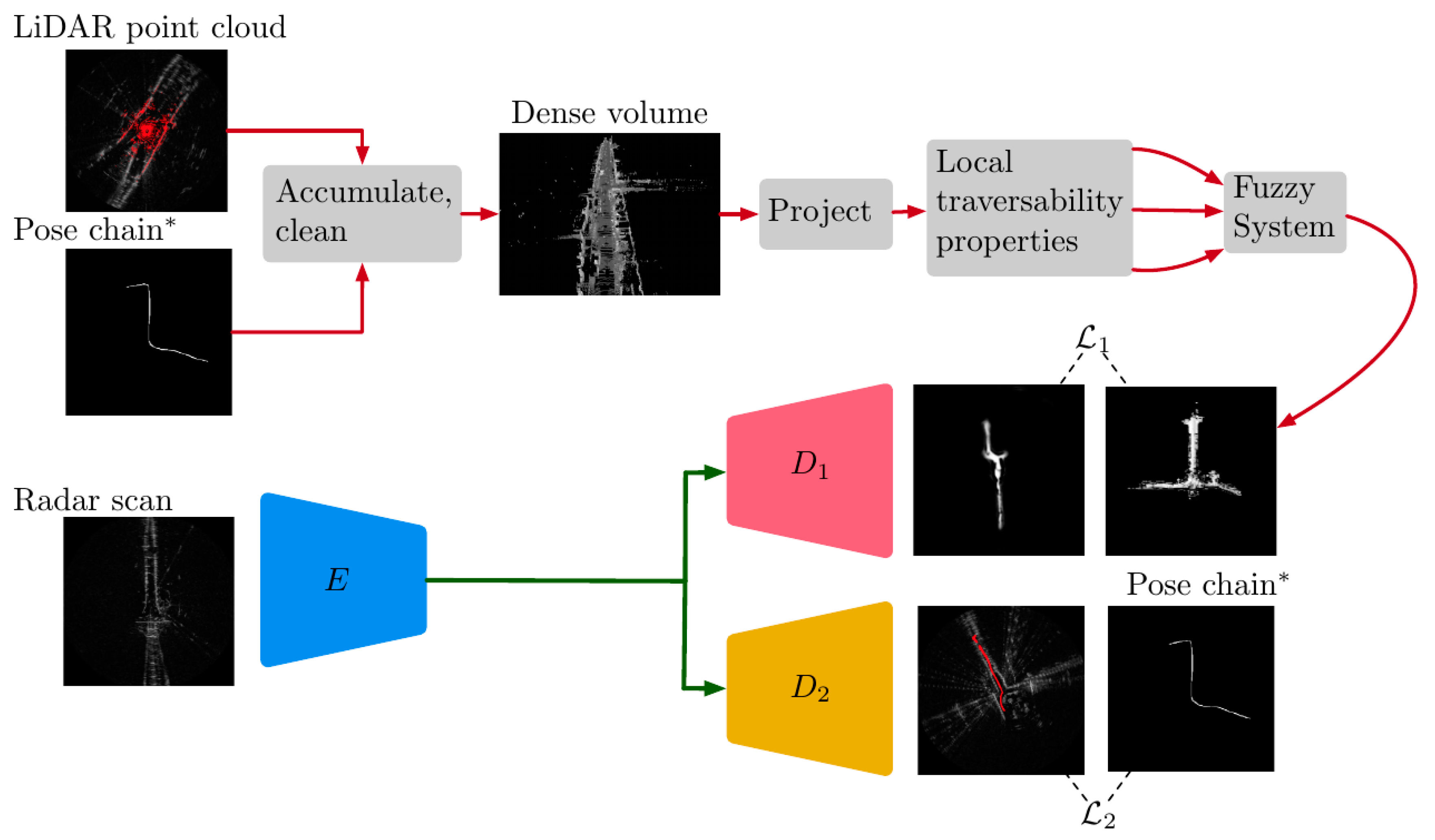
In this paper, we develop several Neural Networt (NN) models and self-supervised learning frameworks to model this problem. Figure 1 illustrates the learned radar model proposed in this paper.
In Section 3 we learn the subtle features in radar that govern traversability (illustrated output of in Figure 1). The proposed method capitalises on radar for robust traversability estimation while avoiding infeasible manual labelling of radar scans by using LiDAR for weak supervision. With this approach, we present a network that can predict continuous traversability maps over a range of 100 using radar alone We demonstrate the use of traversability maps for path proposals in map-less environments through the computation of maximally traversable routes with the graph search algorithm.
In Section 4 path proposal directly from radar frames is learned using an optimised radar odometry ego-motion estimation as ground truth (illustrated output of in Figure 1). Again, we learn this model via weak supervision using recorded ego-motion and applied to route prediction, without the need for arduous manual labelling. We force the feature extractor to learn traversable routes by incorporating the demonstrated ego-motion in a multi-task decoding architecture alongside the traversability maps of Section 3.
The principle contributions of this work are:
- A rules-based system for encoding LiDAR measurements as traversable for an autonomous vehicle (AV),
- An automatic labelling procedure for the radar domain,
- Several learned models which effectively model traversability directly from radar, and
- A joint model which is trained considering traversabile routes which have also been demonstrated by the survey platform.
The rest of this paper is organised as follows. Section 2 places the contribution in the literature. Section 3 describes a self-supervised labelling technique and Neural Network (NN) architecture for learning traversability of the surveyed environment from radar. Section 4 describes a self-supervised labelling technique and NN architecture for learning from radar routes which are demonstrated by the survey vehicle and are also sensed as traversable. Section 5 details our experimental philosophy which is used in Section 6 to analyse and discuss the efficacy of the various proposed models. Section 7 summarises the contribution and Section 8 suggests further avenues for investigation.
2. Related Work
We discuss in this section related literature in the fields of radar signal processing, traversability analysis, and route prediction.
Consider, however, as a broad sweep of the available prior work, that state-of-the-art systems using hundreds of hours of driving data to train models which can understand where a vehicle must drive are well developed in the camera domain, such as for [3], and more recently in [4]. The most relevant radar system available currently is that of [5], which is shown only to segment grassy areas from gravel areas—with traversability being dictated by the designers rather than understood by the algorithm through geometry as in this work.
2.1. Navigation and Scene Understanding from Radar
Frequency-Modulated Continuous-Wave (FMCW) radar is receiving increased attention for exploitation in autonomous applications, including for problems related to SLAM [6,7,8,9] as well as scene understanding tasks such as object detection [10], and segmentation [11]. This increasing popularity is evident in several urban autonomy datasets with a radar focus [12,13].
Cross-modal systems [14,15,16] incorporating inertial and satellite measurements, among others, are also being explored. In this work, however, we focus on endowing radar itself with autonomy-enabling scene understanding capabilities.
Most similar to our work is the inverse sensor model presented in [17], in which style transfer networks are used to model—along with a measure of uncertainty—the occupancy of a grid world as sensed by the radar by mapping radar returns to the statistics of the LiDAR measurement (namely mean and variance in height) collected at the same time. While the representation learned in [17] could also, as in our work, be used downstream for planning where to drive, our system is different from [17] in that we map radar returns to several other geometric features which are intuitively related to the drivability of the environment (surfaces, obstacles, etc) around the autonomous vehicle (AV) and in the further inclusion of a route prediction pipeline direclty in the network.
2.2. Traversability Analysis
There are several recent applications of traversability analysis with cameras [18], 3D LiDAR scanners [19,20], and RGB-D sensors [21].
In grid-based traversability analysis, the surroundings are discretised into cells and the traversability of each cell is evaluated through a set of geometric parameters that model the ground [22,23,24]. Such representations are popular due to their suitability to graph-based route planning algorithms, but use a binary classification and so fail to provide the more detailed and informative representation of continuous scores.
Appearance-based traversability analysis methods based on vision sensors use material classification techniques to incorporate predicted material properties in traversability analysis [25]. Other visual appearance-based work learns traversability using proprioceptive sensor modalities (sensors that acquire information internal to the system) for labelling [26,27]. While appearance-based approaches provide richer information of material properties compared to geometric approaches, their performance is heavily dependent upon lighting conditions and they are more susceptible to erroneous traversability results and false positives [28].
Several investigations improved the reliability of appearance features by combining them with geometric features in hybrid schemes via a data fusion framework [29,30,31]. The requirement of multiple sensor modalities at run time increases the cost of hybrid systems and requires an additional data fusion step.
2.3. Route Prediction
There is extensive literature on route proposal using graph search algorithms on grid representations of the environment derived from exteroceptive sensors, including the likes of Dijkstra [32] and A* [33].
Other popular approaches for real time applications, notably Potential field methods [34] and Rapidly exploring random trees [35] do not require mapping of the environment but still require an exteroceptive sensor with depth information.
More recent literature includes path proposal derived from monocular vision sensors, either by image processing techniques [36,37,38]—which often perform poorly in suboptimal conditions—or, more recently, by semantic segmentation using deep learning [3].
In comparison, path proposal based on radar is in its infancy, despite its advantages over both LiDAR and vision. Early work in this area includes [5], where an approach is presented for learning permissible paths in radar using audio data for weak supervision.
3. Learned Traversability From Radar
This section is concerned with the prediction of traversability maps using a learned radar appearance-based methodology derived from geometric features extracted from a supervisory LiDAR signal. As the core idea for representing traversability is presented in Section 3.2, we keep the discussion in Section 3.1 free of notation. In essence, this section describes the red training data preparation paths illustrated in Figure 1.
3.1. Training Data Generation
Here we describe how the data stream from a pair of LiDAR sensors is collected and pre-processed as a “traversability volume” (Dense volume in Figure 1) before conversion into 2D traversability maps using the geometric interpretation of traversability which will follow in Section 3.2. In this way, data labelling is automated, allowing for the production of training data at large scale. Before describing this self-supervised labelling procedure, however, we first briefly list in Section 3.1.1, Section 3.1.2, Section 3.1.3, Section 3.1.4 and Section 3.1.5 some considerations that must be made in preprocessing the point clouds measured by the pair of LiDARs in order to yield a high quality supervisory signal for the radar model which will be learned in Section 3.3. Section 3.1.1, Section 3.1.2 and Section 3.1.3 are the first accumulation steps and in particular are methods which are implemented with UNIX timestamps and odometry (c.f. Section 5) alone (albeit with a view to better point cloud construction). Section 3.1.4 and Section 3.1.5 in contrast, operate directly on the LiDAR returns which have been accumulated around the position of the test vehicle through the steps described in Section 3.1.1, Section 3.1.2 and Section 3.1.3.
3.1.1. Pose-Chain Accumulation of a Dense Point Cloud
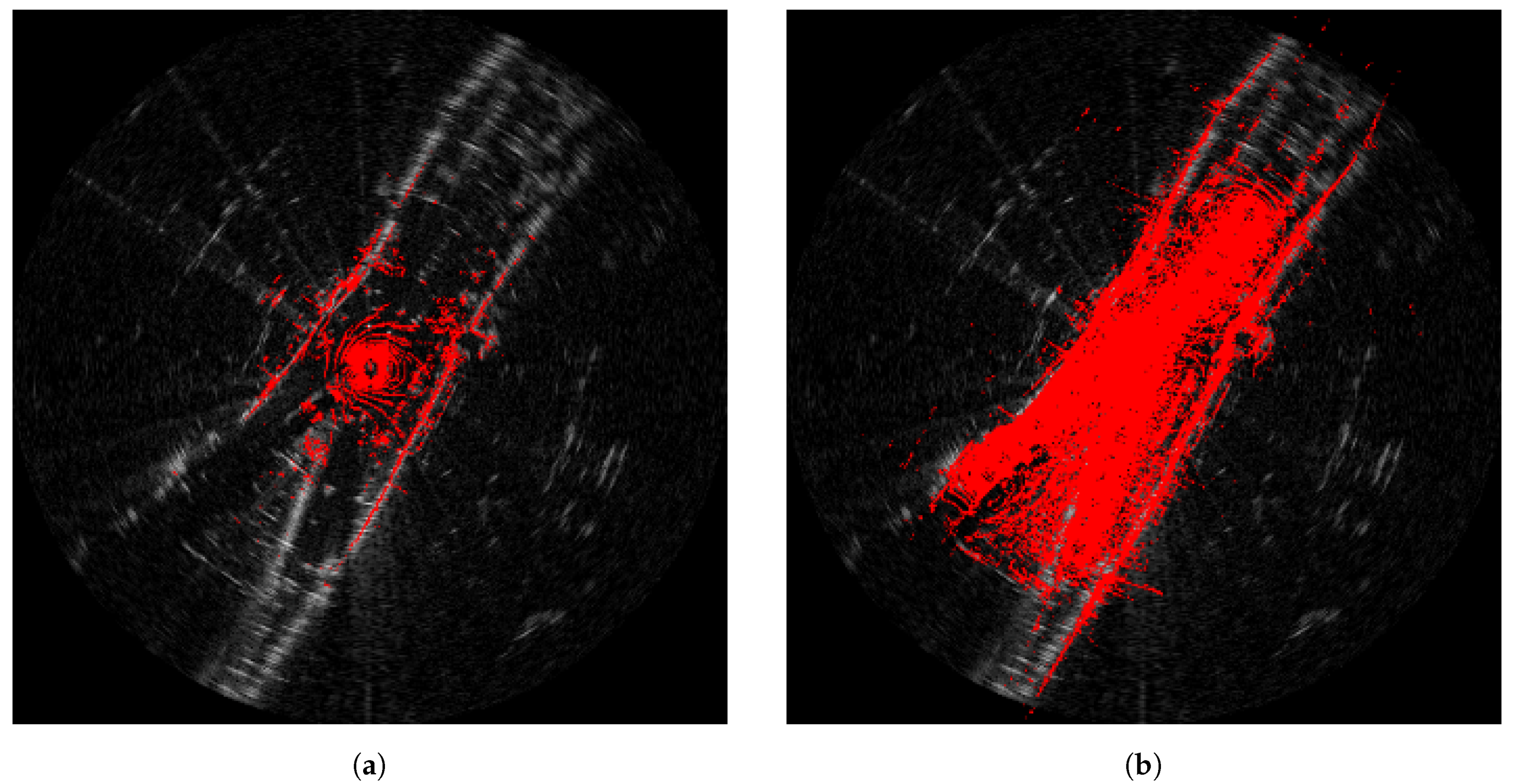
The LiDAR scanning behaviour results in sparse point clouds. Furthermore, the Frequency- Modulated Continuous-Wave (FMCW) radar range far exceeds the feasible range of LiDAR. To address these issues, a dense point cloud is accumulated along a pose-chain constructed with the ego-motion of the test vehicle. Figure 2 illustrates the benefits of a spatial accumulation (in metric space, around the instantaneous pose of the vehicle) in comparison to a single LiDAR scan—providing a richer and denser representation of the environment, as well as covering a larger area.
3.1.2. Spatial Downsampling of the Accumulated Dense Point Cloud
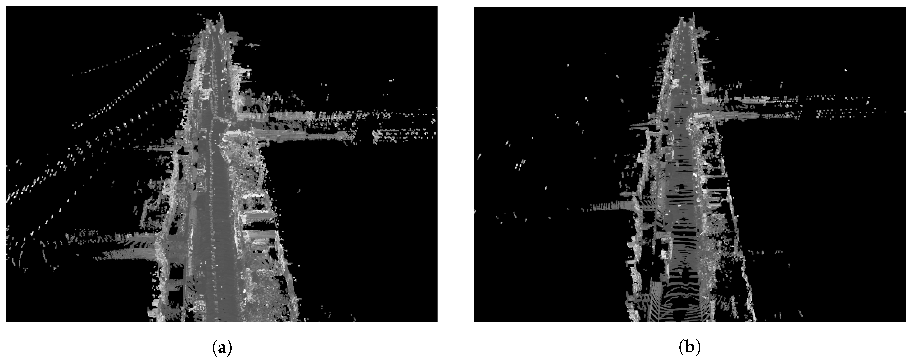
As LiDARs typically operate with a rapid scan rate, this step is taken to offset the computational cost of processing large numbers of point clouds which are accumulated as per Section 3.1.1 above during the (relatively) low scan time of the Frequency-Modulated Continuous-Wave (FMCW) radar. Oversampling also introduces more erroneous data into the accumulated dense point cloud, and leads to greater numbers of duplicated dynamic obstacles. Here, spatial downsampling is applied in order to remove all LiDAR scans occurring within a thresholded distance of the previous can. A value of 10 is found to perform well, with larger values leading to unsatisfactorily sparse dense accumulated point clouds, and smaller values being too computationally expensive to process in the steps which are described below. Figure 3 illustrates the benefits of downsampling the LiDAR timestamps in this way.
3.1.3. Selectively Pruning the Dense Accumulated Point Cloud
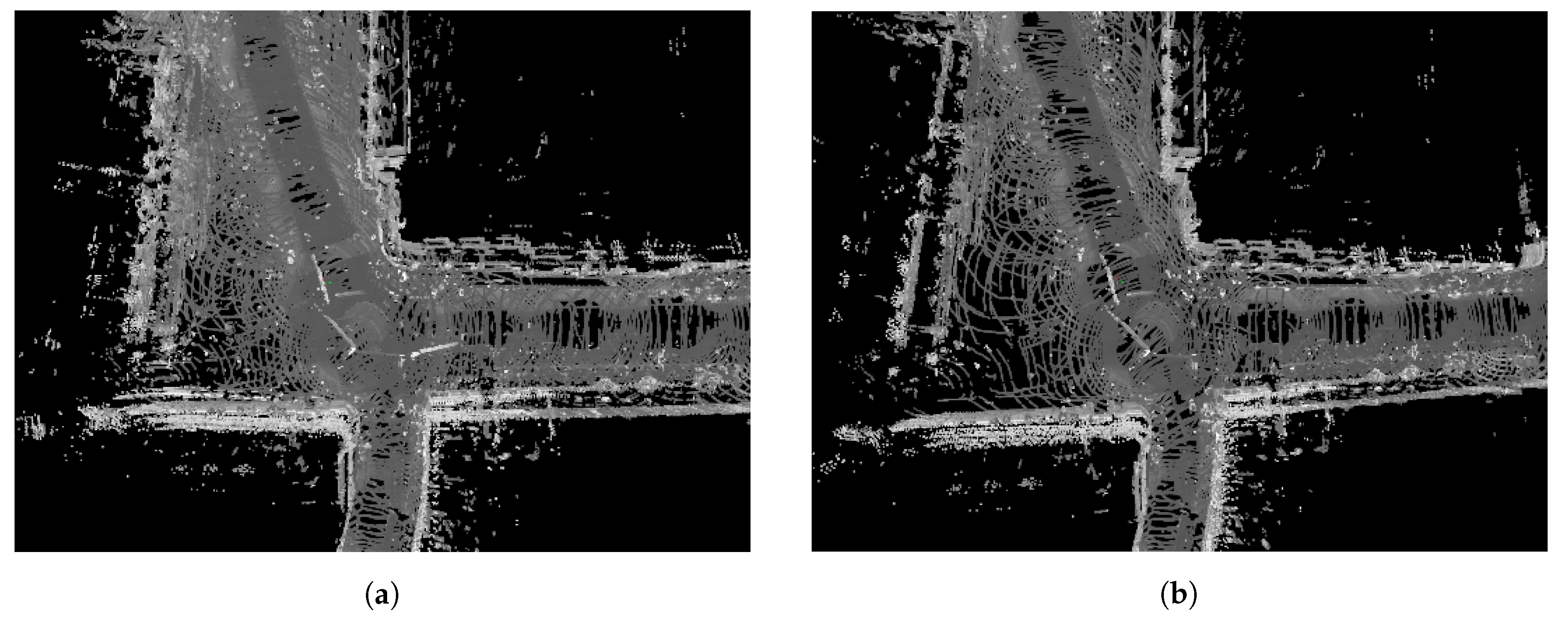
Performing multiple traversals of the same area can lead to problems. Firstly, when the ego-motion returns to the same stretch of road, the resulting point clouds show poor alignment with those from the initial traversal due to drift. Secondly, different obstacles are likely present at different times of traversal, leading to the superposition of false phantom obstacles with the obstacles present at the time of capture of the radar scan. To remedy this problem, “pruned” scans are selectively removed from the accumulated point cloud. Pruned scans are defined as those for which there is at least one other scan within a threshold distance away. The threshold is chosen to be less than the linear motion threshold of Section 3.1.2 above to ensure any poses satisfying the condition are from different traversals of the area. For every pair of scans at distances no more than this thresholded distance in an accumulated dense point cloud (calculated at low cost using k-d trees), the scan collected at a time closest to the query scan time is selected as the surviving scan. With this method, it is ensured that no area of the environment is sampled more than once and the point clouds sampled closest in time to the radar scan are preserved, helping to minimise the impact of any environmental time variance. For this work a value of was found to give good performance. Figure 4 shows the benefits of pruning the dense accumulated point cloud in this way.
3.1.4. Segmentation-Based ICP for Registering Multiple Traversals
Due to the compression of 3D information into a 2D plane by the nature of the radar scan formation process, no roll or pitch information accompanies the odometry transformations which are taken from the dataset to be detailed in Section 5.2) and which are used as in Section 3.1.1, Section 3.1.2 and Section 3.1.3 above. As a result, the accumulated point clouds exhibit a degree of misalignment that would corrupt any computation of traversability (c.f. Section 3.2 below).
An iterative closest point (ICP) algorithm is therefore used to better align the point clouds before further processing, providing a local least squares optimal alignment. The impact of standard iterative closest point (ICP) registration is presented in Figure 5, where alignment of the road is much improved. However, standard (ICP) of this kind implicitly assumes that point clouds which are neighbours in time are also neighbours in space. This assumption breaks down when using traversals collected upon revisiting the area, as is true in our case.
A more robust segmentation-based algorithm is therefore used. Figure 6 illustrates the benefits of this approach. Here, the method can be briefly described as segmenting point clouds into associated traversals (e.g., first visit, second visit, etc) and registering each segment to an “origin” segment which is taken in this work without loss of generality to be the first visit.
3.1.5. Removal Of Duplicate Dynamic Obstacles
Dynamic obstacles undergo transformations between consecutive LiDAR scans, so appear at different poses for each point cloud in the dense accumulated point cloud. Consequently, duplicate dynamic obstacles appear at regular intervals in the point clouds. The voxel-based approach from [39] is applied to remove duplicate dynamic obstacles. Their algorithm segments dynamic and static obstacles in LiDAR point clouds using the following steps:
- Ground plane fitting and Ground vs. obstacle segmentation using three point random sample consensus (RANSAC). An outlier ratio is determined experimentally as 0.46—taking an average over 10 randomly selected point clouds and a conservative number of 50 trials is used to ensure convergence.
- Voxelisation of obstacle point clouds. Each point cloud in the obstacle point cloud set is voxelised with a fine voxel side length of .
- Static vs. Dynamic segmentation. An occupancy grid representing the number of points in each voxel is constructed. The contents of all static voxels are combined with those points in the ground plane to yield a point cloud containing only static obstacles.
This voxel-based approach provides another advantage, acting as a spatio-temporal filter that removes any erroneous data points that are not wide-baseline visible.
Figure 7 illustrates the benefits of this step.
3.2. Traversability Labelling
In an intuitive and qualitative sense, the definition of traversability is clear: traversable terrain may be traversed by a mobile robot but untraversable terrain may not. In this sense, a segmentation task for terrain traversability using a binary score is a well defined problem. Nevertheless, a crisp distinction between what is traversable and what is not is less representative for what the autonomous vehicle (AV) will experience in a real-world deployment—plenty of surfaces are driveable, but not ideally so—and a continuous traversability score can lead to more robust and effective path-planning policies, enabling more flexible operation. In this light, previous works [5,17] have used generative models to recover categorical representations of traversability from radar scans; this work, in contrast, aims to relax this assumption by directly regressing a continuous-valued traversability score. However, the extension to continuous traversability scores is less clear.
In this section, we process the dense accumulated point cloud which is constructed in Section 3.1 above with several geometric proxies (c.f. Section 3.2.1) for traversability. These are combined in a fuzzy-logic ruleset (c.f. Section 3.2.2) to produce a single scalar “traversability” quantity. Applying this ruleset over the radar sensing horizon produces labels (c.f. Section 3.2.3) which are thereafter used in Section 3.3 to train a model which estimates traversability from radar alone.
3.2.1. Geometric Traversability Quantities
Considering a localised region (e.g., a small-to-medium 3D region in space) in the point cloud which is densely accumulated as per Section 3.1, three metrics (Local traversability properties in Figure 1) of geometry well proven in the literature [22,23,40] as appropriate to representing traversability numerically, namely:
- gradient,
- roughness, and
- maximum height variation.
The local gradient, or more precisely the local maximum directional derivative, captures low frequency oscillations in the terrain, while higher frequencies are represented by the roughness measure. The maximum height range characterises any discontinuities in the terrain which are especially indicative of obstacles.
Before defining these quantities, consider that the definition of a LiDAR bin shall be used interchangeably with that for radar: a discretised cell on the x-y plane containing all returns from a projected volume of space.
Local Gradient
To obtain the gradient of a bin , a plane is fitted to its component LiDAR points via least squares regression and its maximum directional derivative calculated. The linear system is formed for a offset normalised plane where each row is such that and . Since the number of points in a bin is typically greater than the number of degrees of freedom of rotation, this is an over-determined system which may be solved using the left psuedo-inverse
After solving for the normal, the maximum directional derivative may be found. The directional derivative of z is defined as , where is a unit vector in a specified direction. By definition, the direction which maximises the directional derivative is that of the gradient vector , leading to the equation
where represents an infinitesimally small displacement in the x-y plane.
Local Roughness
Knowledge of the ground plane offset and normal is sufficient to compute the roughness of a bin, defined as the variance of the distance of points to the ground plane. Assigning as the distance of point to a plane with normal and offset d, distances may be evaluated using the equation
For efficient computation, the numerator of 3 is recast as where resulting in distance vector .
Local Maximum Height Variation
The local maximum height variation
is evaluated as the range of point positions in the vertical axis.
3.2.2. Fuzzy Logic Data Fusion
With three metrics for terrain geometry as defined in Section 3.2.1 above, we now fuse them into a single measure of traversability (Fuzzy System in Figure 1). Performing this step in a mathematically rigorous manner is not straightforward, and relies on assumptions about both the importance of each metric and its scale. Fuzzy logic provides a suitable framework for handling such problems, allowing a well defined and clear translation of system knowledge to input-output behaviour, and has seen use in many branches of engineering, from control theory [41] to medical decision making [42], and multi-sensor data fusion [43].
Here we describe the fuzzy system we propose to encode the geometric quantities related to traversability as discussed above.
Fuzzy Sets
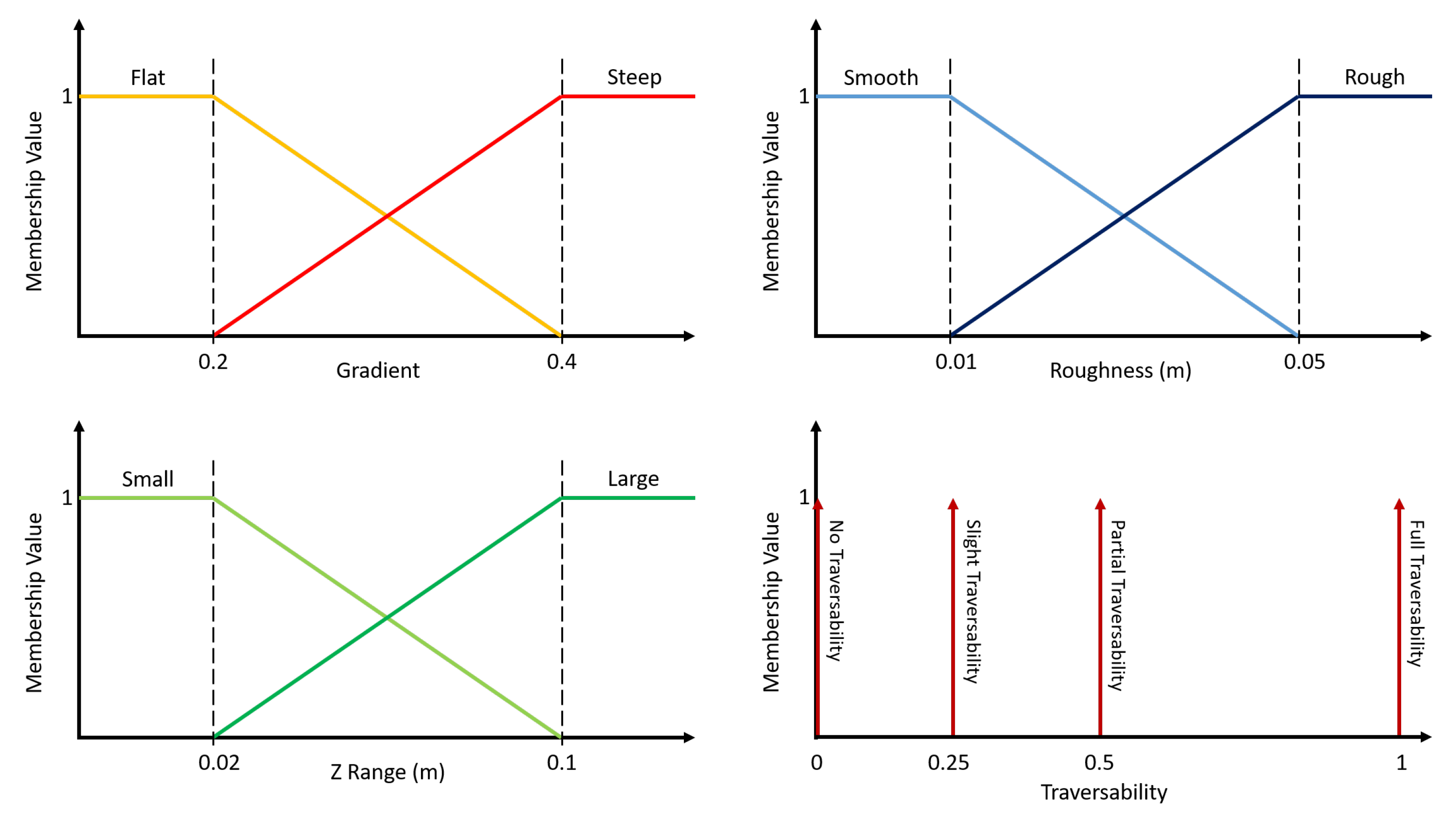
All gradients up to 0.2 are defined as flat and all gradients above 0.4 are defined as steep, corresponding to angles of 11 and 22 respectively. All bin roughness measures up to are considered smooth and all those above as rought. All height ranges up to as small and above as large. Delta function membership functions are assigned to the traversability output sets to simplify the later step of defuzzification. The resulting membership functions are represented graphically in Figure 8 (top left and right, bottom left).
Membership Value
A rule base is required to map each combination of input set instances to output set membership values. The maximum number of rules scales poorly with the number of metrics as well as with the number of sets per metric. Therefore, we propose and use the membership value in the bottom right of Figure 8. The approach that any undesirable set instance results in Partial Traversability, and any two results in No Traversability is taken. The rule IF Steep AND Rough AND Small THEN Slight Traversability is the only exception, where a small height variation indicates a lack of obstacles despite being steep and rough, suggesting some degree of traversability. In doing so, it is imposed that height range has the most influence on traversability due to the implication of obstacles.
3.2.3. Traversability Labels
Here, we finish the description of the self-supervised automatic labelling procedure by describing specific parameterisation used in calculating the geometric quantities as per Section 3.2.1 on the dense point cloud accumulated as per Section 3.1 above.
Voxelisation
For a reliable measure of the maximum directional derivative using least squares, it is necessary to use larger bin sizes to smooth out the effects of sensor noise and registration inaccuracies. In contrast, for good obstacle localisation by the height range metric smaller voxels are desired, so voxelisation with different voxel dimensions is performed for each metric. Larger voxels of side length are used to compute the gradient metric and roughness and smaller voxels of side length are used to compute the height range metrics. The outputs of this step are three matrices representing gradients, roughnesses and height ranges, of (square) dimensions 135, 135, and 270 respectively. It is therefore necessary to upscale the gradient and roughness arrays by a factor of 2 for consistency with the resolution of the height range array.
Data Fusion
With representations of all three metrics, fuzzy logic data fusion (c.f. Section 3.2.2) can be performed on each bin in turn to produce traversability maps of dimension (see Examples below). The scale of the traversability maps do not correspond to that of radar, due to a difference in the distance represented by each bin, analogous to use of a different unit of distance. The multiplicative factor required to scale the traversability maps to correspond to radar is determined using the bin sizes of radar and LiDAR. The Cartesian Frequency-Modulated Continuous-Wave (FMCW) radar scans are configured with a bin size of , whereas the traversability maps are configured for a maximum range of 150 with 135 bins resulting in a bin size of . Consequently, a scaling of 12 is applied to the traversability maps for agreement with radar.
Examples
Consider examples of the output of this traversability labelling pipeline in two different types of typical urban scene. In Figure 9, a sample of traversability labels are presented for radar scans containing junctions and in Figure 10, traversability maps containing large open areas are presented. The output of the Fuzzy System in Figure 1 also shows a traversability label example.
3.3. Single-Task Traversability Network
Here we describe the first of the proposed learned models in this paper, which is trained to predict online the measure of traversability defined in Section 3.2 from the radar measurement.
3.3.1. Neural Network Architecture
The U-Net convolutional neural network (CNN) architecture [44] is used as the base architecture for this and the models which follow in later sections (c.f. Section 4). This model corresponds to the encoder-decoder path shown in Figure 1 which is formed by (blue and red).
The intuition behind U-Net is the capture of features with high semantic meaning—but low resolution—using the encoder and their enrichment with high resolution features through skip connections. The same intuition is applied to traversability prediction; encoding contextual information about terrain traversability into a compressed representation then upsampling to achieve a sharp traversability map.
3.3.2. Learned Objective
In the application of this work, traversability scores of floating point form are required and as such a sigmoid layer is appended at the decoder output to constrain all outputs to lie in the range . The loss (c.f. Figure 1) is thus computed as the mean squared error (MSE) between the prepared labels and predicted traversability scores over the radar grid as shown in Figure 1. To learn this objective we use stochastic gradient descent (SGD) with momentum.
3.3.3. Data Augmentation
In urban environments, there is a strong correlation between the orientation of the test vehicle and the orientation of the road. Roads are designed to be traversed in either of two directions. However, it is less common for a vehicle to be orthogonal to the direction of travel—a situation usually only arising at junctions. As a consequence, there is a bias in the dataset we train and test on (c.f. Section 5.2) for traversable regions to extend vertically down the centre of the radar scan, representing the forward and backward directions in the radar coordinate system. The traversability model should generalise well to different directions and thus provide a direction-invariant response to input radar scans. To help remove this bias, a random rotation in the range is applied to each Cartesian radar scan and its associated traversability label during training. This step also reduces the correlation between radar scans which are near in space, so network training better adheres to the assumption of independent identically distributed data that is implicit during optimisation of the Neural Network (NN).
3.3.4. Training Configuration
To satisfy VRAM constraints, a small batch size of two is used with a low learning rate of 0.0015 to help ensure convergence on a local minimum.
4. Learned Route Proposals From Radar
In this section we use the ego-motion of the test vehicle to learn the driving behaviour of humans. This is developed for the first time in this work for the radar domain in a manner similar to that applied in [3] for visual cameras.
4.1. Training Data Generation
The ground truth odometry from the Oxford Radar Robotcar Dataset (c.f. Section 5.2 below) is used to produce a Cartesian mask of of the same dimensions as the radar scan where all radar bins that fall within the recorded route are labelled with 1 and all those that did not are labelled 0. In this manner, large quantities of training data are generated that capture expert human driving knowledge without the need for manual labelling. The rest of this section provides the necessary details for implementation of this simply described labelling procedure.
4.1.1. Pose Chain Construction
In a manner similar to that of Section 3.1.1, we accumulate all timestamps visited by the test vehicle within a range of the centre of the radar scan. Since only the most likely route should be proposed, a temporal search of the available odometry timestamps is applied (rather than the spatial search applied in Section 3.1.1). In doing so, we collect timestamps from a single traversal only.
To ensure consistency between labels, a distance constraint is placed on the position of poses. Only poses lying within 130 of the origin pose—as measured along the route—are kept, thus supervising the network (c.f. Section 4.2 below) to propose routes of consistent length. Routes of length 130 traverse a significant proportion of the radar scan, helping to make maximum use of the large radar sensing horizon available (about 165 ).
4.1.2. Spline Interpolation
Spline interpolation is performed between the poses collected along the pose chain as per Section 4.1.1. A linear interpolating spline is used to model the motion of the vehicle and, in doing so, allow the computation of a function that describes the motion of the vehicle.
In this manner, the set of discrete poses are mapped to a continuous route through the area measured by the radar scan. Here, s denotes cumulative distance travelled from the first (origin) pose and is the position vector of the vehicle. Since the route taken by the test vehicle may present as any arbitrary curve in the -plane, it is necessary to express the interpolating spline as a function of vehicle displacement, s.
Therefore, two separate splines are fitted to the x and y components of ego-motion with respect to a third variable, allowing arbitrary paths in the x-y plane. The vehicle displacements are calculated as the cumulative sum of the root of squared x and y coordinate differences, according to
where is initialised to 0. A dense set of vehicle positions is then retrieved by interpolating points with a linear spline. A linear spine is a suitable choice for this dense set due to the low computational cost of linear interpolation compared to the quadratic or cubic spline counterparts, while still providing a path which appears smooth to the eye.
For consistency between routes of different length, the cumulative displacement is normalised by the total cumulative sum of all relative poses, resulting in a route function of the form .
4.1.3. Pixelwise Segmentation of the Moving Vehicle Wheelbase
In the final stage of the route labelling pipeline, a radar mask is produced from the function , whereby all bins intersected by the route are labelled with a value of 1 and all others 0. The resulting mask contains a route segment of only one bin width, which would provide a weak supervision signal and not accurately represent the dimensions (wheelbase) of the test vehicle. Stated alternatively, the route corresponds only to the positions of the Frequency-Modulated Continuous-Wave (FMCW) radar sensor itself, analogous to treating the car as a zero dimensional point. This is corrected for by labelling all bins within a neighbourhood of the route bins with a value of 1, increasing the apparent width of the route segment to , inline with the track width of typical vehicles.
4.1.4. Route Labels
A sample of route labels generated by the proposed labelling algorithm are presented in Figure 11 and Figure 12 for scenes encountered by the test vehicle featuring junctions and open areas, respectively. Please note that these route labels are of the same resolution as the traversability labels described above and shown in Figure 9 and Figure 10 as well as the radar scans themselves, which is important in the final architecture to be discussed later in Section 4.2. Note also that learning route proposals in the fashion proposed in this section makes no account for whether the route traced out in the radar scan is traversable. This is to say, the labelled radar scan only represents the environment as measured at one instant along the route, and it is possible that the labels pass through objects or sensor artefacts. We address this in Section 4.2 by forcing the encoder to learn demonstrated routes which are also traversable.
4.2. Multi-Task Traversable Route Prediction Network
In this section, we detail the application of the labelling pipeline described in Section 4.1.4 to the training of a Neural Network (NN) for route proposal. In this way, a weak supervision approach is used to learn the driving behaviour of humans.
However, this route prediction network is initialised with parameters obtained from the the traversability prediction to provide a better initialisation state for training. The intuition here is that drivable routes are by definition traversable. Since Neural Network (NN) are highly non-linear, providing a better initialisation state is expected to allow convergence on a lower and better performing local minimum, while biasing the network to avoid obstacles and select high traversability routes. Specifically, the learned radar features that encode route viability are expected to have a strong dependency on those features which encode traversability.
4.2.1. Neural Network Architecture
As before (c.f. Section 3.3.1), the U-Net architecture is applied to this task. This model corresponds to the encoder-decoder path shown in Figure 1 which is formed by (blue and orange). As with Section 3.3, a sigmoid output layer is added to the output of the network decoder to ensure output bin values in the range , representing confidences in the proposed route.
4.2.2. Learned Objective
Since route proposal is a segmentation task, the loss function (c.f. Figure 1) is a summation of the loss and soft dice loss functions. A disadvantage of binary cross-entropy (BCE) is that it takes an average of values calculated for each voxel, making it susceptible to the level of class-imbalance seen in Figure 11 and Figure 12. Indeed, the proposed route should be based on the features in the radar scan rather than just a leaned prior distribution of route voxels, so this is undesirable. For example, the loss could be decreased simply by reducing the number of voxels segmented in the route set, regardless of the features in the radar scan where they lie. In addition, since loss is computed voxel-wise, cross entropy fails to capture the relationships between voxels.
These disadvantages are often mitigated using a weighting scheme to scale the loss associated with distinct ground truth classes differently, compensating for the effects of class-imbalance. However, the soft dice loss provides a measure of overlap between sets which is particularly important for the accurate prediction of segment boundaries [45]. This loss captures important global information missed by binary cross-entropy (BCE). In this way, the dice coefficient is robust to class-imbalance because it considers the ratio of the total number of correctly predicted route voxels to the total number of route voxels – a measure normalised by class incidence.
The loss (c.f. Figure 1) therefore considers both local and global similarity.
In Section 6 we consider training networks which include just the single encoder-decoder path with (demonstrated routes alone) as well as both encoder-decoder paths with and (traversability labels and demonstrated routes) and show that the latter approach is superior.
4.2.3. Data Augmentation
Due to the bias of road orientation discussed in Section 3.3.3, a random rotation in the range is applied to each item in the training data. The position of the vehicle on the road during this step must also be considered, since any rotation of the radar scan and route mask pair greater in magnitude than will result in an apparent change in vehicle position relative to the road. In the United Kingdom (UK) (c.f. Section 5.2 for a description of the dataset) vehicles are required to drive on the left side of the road. This rule of the road should be observed during data augmentation. This is not the case for a random rotation, where any rotation greater than in magnitude transforms the route mask to the right side of the road. This is addressed by reflecting both the radar scan and route mask about the x axis after any rotation greater in magnitude than . This transforms the route mask back onto the left side of the road, ensuring consistency in the route masks.
4.2.4. Training Configuration
Stochastic gradient descent (SGD) is used to optimise using a batch size of 2 and a low learning rate of 0.0015.
The network is presented with Cartesian radar frames of dimension and route masks of equal dimension, representing a downsampling of three times from the raw radar scan resolution to satisfy graphics processing unit (GPU) VRAM constraints, as described in Section 3.3.
5. Experimental Setup
The experiments are performed using data collected from the Oxford RobotCar platform [46] which is equipped as described in the recently released Oxford Radar RobotCar Dataset [12].
5.1. Sensor Suite
Our data collection platform is pictured in Figure 13a.
A CTS350-X Navtech Frequency-Modulated Continuous-Wave (FMCW) scanning radar operating at 76 to 77 with a beam-width of is used. It offers a full 360 field-of-view (FOV). Range is discretised into 3768 bins, providing a resolution of at each of 400 azimuth angles about an axis perpendicular to the ground—representing an angular resolution of 2. Scans are performed at a sampling frequency of 4 .
In contrast, a Velodyne HDL-32E 3D LiDAR provides a sampling frequency of 20 with a horizontal field-of-view (FOV) of 360 and a vertical field-of-view (FOV) of . The point clouds are constructed using 32 stacked laser planes and achieve a maximum range of 100 compared to 165 for radar.
5.2. Dataset
Here we describe the dataset used to train and evaluate our system.
5.2.1. Ground Truth Odometry
For preparing the pose chain along which the dense accumulated point cloud is constructed and preprocessed (c.f. Section 3.1.1, Section 3.1.2 and Section 3.1.3), we use the ground truth odometry described in [12] which is computed by a global optimisation using Global Positioning System (GPS), robust Visual Odometry (VO), and visual loop closures.
5.2.2. Dataset Splits
The Oxford Radar Robot Dataset [12] is partitioned according to Figure 13b, which represents relative proportions of training, validation and test data of 88%, 5%, and 7% respectively. In doing so, one of the approximately 9 trajectories in the Oxford city centre was divided into three distinct portions: train, valid, and test. Figure 13b shows the Global Positioning System (GPS) trace of the trajectory. The test split was specifically selected as the vehicle traverses a portion of the route in the opposite direction and exhibits interesting junctions. The valid split selected was quite simple, consisting of two straight periods of driving separated by a right turn, and was used for automatic selection of the checkpoints deployed for testing on the test split (c.f. Section 5.3 below).
5.3. Model Selection
We describe here some aspects of the training of each of the three proposed models.
5.3.1. Traversability Model
Consider the first model deployed: the traversability model of Section 3. Training was run for a total of 26 epochs over which the loss is evaluated over the valid partition of the dataset. This validation loss is seen to level off after epoch 15, though fluctuations—attributed to the small batch size—do remain. Epoch 22 is selected for the traversability model because it minimises the loss on the validation set.
5.3.2. Traversable Route Prediction Model
Consider the second model deployed: the traversable route prediciton model of Section 4. Training was run for a total of 86 epochs. The validation loss is minimised at epoch 59, after which it increases due to over-fitting of the training data. Consequently, the network state at epoch 59 is selected for the combined model.
5.4. Compute Hardware
Our system is fairly lightweight, capable of average frame rates of (including all memory transfer and data parsing overheads) on an Nvidia RTX 2060 graphics processing unit (GPU), allowing for potential real-time applications.
6. Results and Discussion
This section describes the observed performance of the two models described in Section 3 and Section 4 in the experimental setup described in Section 5.
6.1. Traversability Predictions
Here we evaluate the facility of our learned feature extraction at retrieving information from radar scans regarding the traversability of the scanned environment.
A sample of traversability maps inferred for radar scans in the test portion of the dataset (c.f. Section 5.2) using this first network with weights equal to those at the chosen epoch (c.f. Section 5.3) are presented in Figure 14 and Figure 15, representing cases which are challenging due to radar artefacts and unusual road layout respectively.
6.1.1. Sensor Artefacts
In Figure 14, repeated reflections of the millimetre-wave (MMW) radiation result in duplicate roads running parallel to the real road in the radar scans, presenting a challenge for this traversability prediction network. In Figure 14a,d we observe that the traversable area of the sensed environment does not extend out to the duplicate road boundaries manifested by this sensor artefact. In Figure 14b,e the street is narrower than in Figure 14a,d, which the radar-to-traversability model has no problem understanding. This is an indication that the network has not learned to yield a fixed size area around the centre of the scan (the vehicle location) as traversable. In Figure 14c,f, even though not visible to the human eye in the radar scan, a wide open area (top right of the frames) is understood to be traversable.
6.1.2. Unusual Road Layout
In Figure 15, the radar frames captured near to the roundabout suffer from occlusion but the traversability labels are not affected—at least insofar as they are useful for local environment perception. Comparing Figure 15a,d against Figure 15b,e or Figure 15c,f, it is clear that the “occlusion” effect is caused by something in the top-right (in the frame of reference of Figure 15a,d) of the turn that the vehicle is navigating.
6.1.3. Traversability Planning
The utility of the radar traversability predictions may be further evaluated by the optimally traversable routes they imply. Indeed, the traversability map data representation is equivalent to a vertex-weighted graph, so it is suitable for the application of graph search algorithms for path planning. The performance of A* route planning for several challenging radar frames is therefore presented in Figure 16—indicating the utility of the traversability maps learned by this first model. However, any route inferred from the predicted traversability maps should satisfy the motion constraints of the vehicle and influenced by obstacles—for example, by showing some degree of smoothness. In this sense, the planned paths shown in Figure 16 are slightly jagged, and would not be suitable without smoothing for direct use in controlling the motion of an autonomous vehicle (AV). Section 6.2 shows smoother inferred paths which are learned end-to-end as per Section 4.
6.2. Traversable Route Prediction
A sample of path proposals evaluated for radar scans in the test partition of the dataset is presented in Figure 17 and Figure 18.
Generally, the paths inferred by this multi-tasking network configuration (c.f. Section 4) are smoother and broader than those shown for the single-task network configuration (c.f. Section 3), as compared to the A* search results discussed in Section 6.1 and shown in Figure 16 above. The routes show a high degree of smoothness and reliably navigate around obstacles. Most importantly, as compared to Figure 16, we are able through the joint network configuration to predict several likely paths for the autonomous vehicle (AV) to take, rather than only the maximally traversable.
The model deployed in Figure 17 was trained only using route labels (c.f. in the learned objectives of Section 4.2.2). The model deployed in Figure 18—in contrast—was trained using traversability maps as well as route labels (c.f. and in the learned objectives of Section 4.2.2).
In Figure 18a as compared to Figure 17a, the proposed vehicle track stays consistently wide. We see similar performance in Figure 18b as compared to Figure 17b—suggesting that straight urban canyons are equally easily to understand by and as compared to alone. In Figure 18e as compared to Figure 17e, gaps in the proposed routes are not as evident. In Figure 18d as compared to Figure 18d, both options for the next manoeuvre are complete—or more perfectly understood by the model as traversable and potential paths.
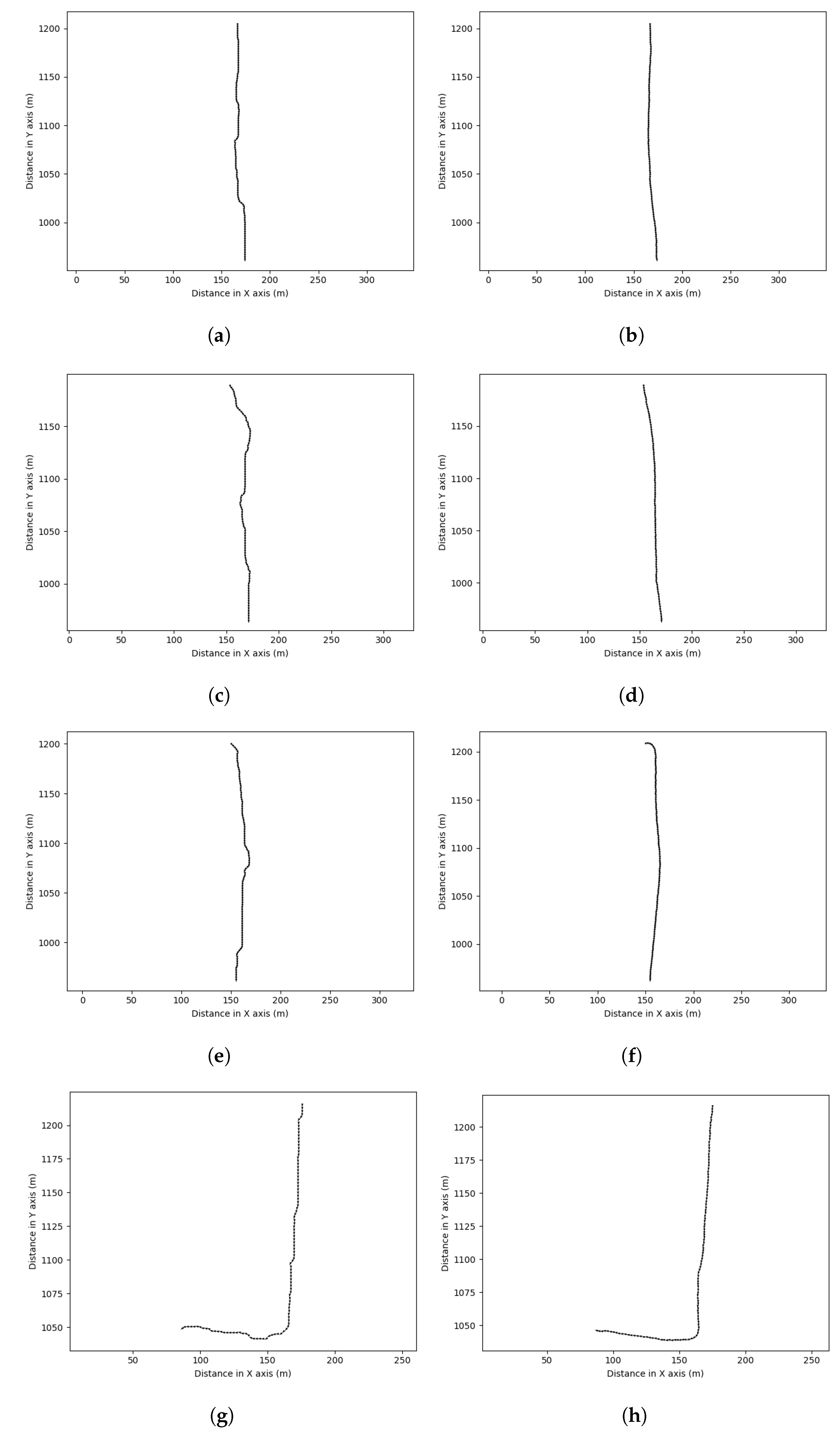
Consider Figure 19; here, each frame shows a planed route for the vehicle to follow. The left examples are the result of an A* search in the inferred traversability map. The A* search is performed in the pixel space of this traversability map. For comparison, therefore, and to format the inferred routes from the combined architecture (e.g., Figure 18), we apply a thinning technique – specifically the Medial Axis Transform (MAT) [47]—to reduce the proposed routes to a pixel width. A pruning process is applied to the thinned route to remove unwanted spurs. Specifically, the longest path through the skeleton is evaluated and all other branches are removed. The proposed routes are suggested by the network natively, whereas A* requires a start and goal location. For fair comparison, therefore, the A* search was initiated and terminated at the endpoints of the thinning procedure described above. What is found is that the proposed routes learned by including vehicle demonstration (c.f. Section 4) are qualitatively smoother and more suitable for the feasible kinematics of the vehicle (i.e., the jittering orientation changes and small lateral jumps are not an ideal aspect of the A* plans).
Lastly, routes are proposed at an average rate of (including all memory transfer and data parsing overheads) making them suitable for real-time applications.
7. Conclusions
In this work, an appearance-based radar traversability methodology was introduced and shown to infer traversability maps that are robust to occlusion and artefacts while exceeding the range of existing vision and LiDAR methodologies. The computation of maximally traversable routes through the application of graph search algorithms on inferred traversabilty maps was shown to be a robust method of path planning over long ranges. Furthermore, a weak supervision approach using LiDAR traversability labels generated via a geometric traversability analysis has been shown to be a robust and scalable means to train radar appearance methodologies without the requirement for manual labelling. In an extension to traversability analysis, an end-to-end radar path proposal system was presented and shown to propose paths that reliably navigate around obstacles. The final form of the system we propose employs joint learning by the encoder of features which can be decoded for both traversability of the scene as sensed by the radar as well as feasible routes demonstrated by the survey vehicle. The proposed system is shown to predict smooth, feasible routes in various typical urban driving scenes. We expect that the proposed system will have utility in enabling autonomy in previously unvisited environments (as it is “mapless”) which are challenged by extreme weather and lighting conditions.
8. Future Work
In the future, post-processing methods exist which could improve the performance of the labels provided, notably spatio-temporal filtering using the predictions of neighbouring radar frames.
Author Contributions
Conceptualization, M.B., M.G., D.D.M. and P.N.; methodology, M.B., M.G., D.D.M.; software, M.B.; validation, M.B.; formal analysis, M.B.; investigation, M.B.; resources, P.N.; data curation, M.G.; writing—original draft preparation, M.B. and M.G.; writing—review and editing, M.B., M.G. and D.D.M.; visualization, M.B.; supervision, M.G., D.D.M. and P.N.; project administration, P.N.; funding acquisition, P.N. All authors have read and agreed to the published version of the manuscript.
Funding
This project is supported by the Assuring Autonomy International Programme, a partnership between Lloyd’s Register Foundation and the University of York and UK EPSRC Programme Grant EP/M019918/1.
Acknowledgments
The authors would like to thank their partners at Navtech Radar Ltd.
Conflicts of Interest
The authors declare no conflict of interest.
References
- Piotrowsky, L.; Jaeschke, T.; Kueppers, S.; Siska, J.; Pohl, N. Enabling high accuracy distance measurements with FMCW radar sensors. IEEE Trans. Microw. Theory Tech. 2019, 67, 5360–5371. [Google Scholar] [CrossRef]
- Brooker, G.; Hennessey, R.; Bishop, M.; Lobsey, C.; Durrant-Whyte, H.; Birch, D. High-resolution millimeter- wave radar systems for visualization of unstructured outdoor environments. J. Field Robot. 2006, 23, 891–912. [Google Scholar] [CrossRef]
- Barnes, D.; Maddern, W.; Posner, I. Find Your Own Way: Weakly-Supervised Segmentation of Path Proposals for Urban Autonomy. arXiv 2016, arXiv:cs.RO/1610.01238. [Google Scholar]
- Sun, Y.; Zuo, W.; Liu, M. See the Future: A Semantic Segmentation Network Predicting Ego-Vehicle Trajectory With a Single Monocular Camera. IEEE Robot. Autom. Lett. 2020, 5, 3066–3073. [Google Scholar] [CrossRef]
- Williams, D.; De Martini, D.; Gadd, M.; Marchegiani, L.; Newman, P. Keep off the Grass: Permissible Driving Routes from Radar with Weak Audio Supervision. In Proceedings of the IEEE Intelligent Transportation Systems Conference (ITSC), Rhodes, Greece, 20–23 September 2020. [Google Scholar]
- Cen, S.H.; Newman, P. Precise ego-motion estimation with millimeter-wave radar under diverse and challenging conditions. In Proceedings of the 2018 IEEE International Conference on Robotics and Automation (ICRA), Brisbane, Australia, 21–25 May 2018; pp. 1–8. [Google Scholar]
- Barnes, D.; Weston, R.; Posner, I. Masking by moving: Learning distraction-free radar odometry from pose information. arXiv 2019, arXiv:1909.03752. [Google Scholar]
- Barnes, D.; Posner, I. Under the radar: Learning to predict robust keypoints for odometry estimation and metric localisation in radar. arXiv 2020, arXiv:2001.10789. [Google Scholar]
- Park, Y.S.; Shin, Y.S.; Kim, A. PhaRaO: Direct Radar Odometry using Phase Correlation. In Proceedings of the IEEE International Conference on Robotics and Automation (ICRA), Paris, France, 31 May–31 August 2020. [Google Scholar]
- Sheeny, M.; Wallace, A.; Wang, S. 300 GHz Radar Object Recognition based on Deep Neural Networks and Transfer Learning. arXiv 2019, arXiv:1912.03157. [Google Scholar] [CrossRef]
- Kaul, P.; De Martini, D.; Gadd, M.; Newman, P. RSS-Net: Weakly-Supervised Multi-Class Semantic Segmentation with FMCW Radar. In Proceedings of the IEEE Intelligent Vehicles Symposium (IV), Las Vegas, NV, USA, 23–26 June 2020. [Google Scholar]
- Barnes, D.; Gadd, M.; Murcutt, P.; Newman, P.; Posner, I. The Oxford Radar RobotCar Dataset: A Radar Extension to the Oxford RobotCar Dataset. In Proceedings of the IEEE International Conference on Robotics and Automation (ICRA), Paris, France, 31 May–31 August 2020. [Google Scholar]
- Kim, G.; Park, Y.S.; Cho, Y.; Jeong, J.; Kim, A. Mulran: Multimodal range dataset for urban place recognition. In Proceedings of the IEEE International Conference on Robotics and Automation (ICRA), Paris, France, 31 May–31 August 2020. [Google Scholar]
- Iannucci, P.A.; Narula, L.; Humphreys, T.E. Cross-Modal Localization: Using automotive radar for absolute geolocation within a map produced with visible-light imagery. In Proceedings of the 2020 IEEE/ION Position, Location and Navigation Symposium (PLANS), Portland, OR, USA, 20–23 April 2020; pp. 285–296. [Google Scholar]
- Narula, L.; Iannucci, P.A.; Humphreys, T.E. All-Weather sub-50-cm Radar-Inertial Positioning. arXiv 2020, arXiv:2009.04814. [Google Scholar]
- Tang, T.Y.; De Martini, D.; Barnes, D.; Newman, P. RSL-Net: Localising in Satellite Images From a Radar on the Ground. IEEE Robot. Autom. Lett. 2020, 5, 1087–1094. [Google Scholar] [CrossRef] [Green Version]
- Weston, R.; Cen, S.; Newman, P.; Posner, I. Probably unknown: Deep inverse sensor modelling radar. In Proceedings of the 2019 International Conference on Robotics and Automation (ICRA), Montreal, QC, Canada, 20–24 May 2019; pp. 5446–5452. [Google Scholar]
- Bekhti, M.A.; Kobayashi, Y. Regressed Terrain Traversability Cost for Autonomous Navigation Based on Image Textures. Appl. Sci. 2020, 10, 1195. [Google Scholar] [CrossRef] [Green Version]
- Zhang, K.; Yang, Y.; Fu, M.; Wang, M. Traversability assessment and trajectory planning of unmanned ground vehicles with suspension systems on rough terrain. Sensors 2019, 19, 4372. [Google Scholar] [CrossRef] [Green Version]
- Martínez, J.L.; Morán, M.; Morales, J.; Robles, A.; Sánchez, M. Supervised Learning of Natural-Terrain Traversability with Synthetic 3D Laser Scans. Appl. Sci. 2020, 10, 1140. [Google Scholar] [CrossRef] [Green Version]
- Yang, K.; Wang, K.; Cheng, R.; Hu, W.; Huang, X.; Bai, J. Detecting traversable area and water hazards for the visually impaired with a pRGB-D sensor. Sensors 2017, 17, 1890. [Google Scholar] [CrossRef] [Green Version]
- Langer, D.; Rosenblatt, J.K.; Hebert, M. A behavior-based system for off-road navigation. IEEE Trans. Robot. Autom. 1994, 10, 776–783. [Google Scholar] [CrossRef] [Green Version]
- Gennery, D.B. Traversability Analysis and Path Planning for a Planetary Rover. Auton. Robot. 1999, 6, 131–146. [Google Scholar] [CrossRef]
- Ye, C. Navigating a Mobile Robot by a Traversability Field Histogram. IEEE Trans. Syst. Man Cybern. Part B (Cybern.) 2007, 37, 361–372. [Google Scholar] [CrossRef]
- Angelova, A.; Matthies, L.; Helmick, D.; Perona, P. Learning and Prediction of Slip from Visual Information: Research Articles. J. Field Robot. 2007, 24, 205–231. [Google Scholar] [CrossRef]
- Helmick, D.; Angelova, A.; Matthies, L. Terrain Adaptive Navigation for Planetary Rovers. J. Field Robot. 2009, 26, 391–410. [Google Scholar] [CrossRef] [Green Version]
- Howard, A.; Turmon, M.; Matthies, L.; Tang, B.; Angelova, A.; Mjolsness, E. Towards learned traversability for robot navigation: From underfoot to the far field. J. Field Robot. 2006, 23, 1005–1017. [Google Scholar] [CrossRef]
- Papadakis, P. Terrain traversability analysis methods for unmanned ground vehicles: A survey. Eng. Appl. Artif. Intell. 2013, 26, 1373–1385. [Google Scholar] [CrossRef] [Green Version]
- Sock, J.; Kim, J.; Min, J.; Kwak, K. Probabilistic traversability map generation using 3D-LIDAR and camera. In Proceedings of the 2016 IEEE International Conference on Robotics and Automation (ICRA), Stockholm, Sweden, 16–21 May 2016; pp. 5631–5637. [Google Scholar]
- Lu, L.; Ordonez, C.; Collins, E.G.; DuPont, E.M. Terrain surface classification for autonomous ground vehicles using a 2D laser stripe-based structured light sensor. In Proceedings of the 2009 IEEE/RSJ International Conference on Intelligent Robots and Systems, St. Louis, MO, USA, 10–15 October 2009; pp. 2174–2181. [Google Scholar]
- Schilling, F.; Chen, X.; Folkesson, J.; Jensfelt, P. Geometric and visual terrain classification for autonomous mobile navigation. In Proceedings of the 2017 IEEE/RSJ International Conference on Intelligent Robots and Systems (IROS), Vancouver, BC, Canada, 24–28 September 2017; pp. 2678–2684. [Google Scholar]
- Dijkstra, E.W. A note on two problems in connexion with graphs. Numer. Math. 1959, 1, 269–271. [Google Scholar] [CrossRef] [Green Version]
- Hart, P.E.; Nilsson, N.J.; Raphael, B. A Formal Basis for the Heuristic Determination of Minimum Cost Paths. IEEE Trans. Syst. Sci. Cybern. 1968, 4, 100–107. [Google Scholar] [CrossRef]
- Khatib, O. Real-time obstacle avoidance for manipulators and mobile robots. In Proceedings of the 1985 IEEE International Conference on Robotics and Automation, St. Louis, MO, USA, 25–28 March 1985; Volume 2, pp. 500–505. [Google Scholar]
- Lavalle, S. Rapidly-Exploring Random Trees: A New Tool for Path Planning. Research Report 9811. 1998. Available online: http://msl.cs.illinois.edu/~lavalle/papers/Lav98c.pdf (accessed on 2 December 2020).
- Zhan, Q.; Huang, S.; Wu, J. Automatic Navigation for A Mobile Robot with Monocular Vision. In Proceedings of the 2008 IEEE Conference on Robotics, Automation and Mechatronics, Chengdu, China, 21–24 September 2008; pp. 1005–1010. [Google Scholar]
- Álvarez, J.M.; López, A.M.; Baldrich, R. Shadow resistant road segmentation from a mobile monocular system. In Proceedings of the Iberian Conference on Pattern Recognition and Image Analysis, Girona, Spain, 6–8 June 2007; pp. 9–16. [Google Scholar]
- Yamaguchi, K.; Watanabe, A.; Naito, T.; Ninomiya, Y. Road region estimation using a sequence of monocular images. In Proceedings of the 19th International Conference on Pattern Recognition, Tampa, FL, USA, 8–11 December 2008; pp. 1–4. [Google Scholar]
- Asvadi, A.; Premebida, C.; Peixoto, P.; Nunes, U. 3D Lidar-based Static and Moving Obstacle Detection in Driving Environments: An approach based on voxels and multi-region ground planes. Robot. Auton. Syst. 2016, 83. [Google Scholar] [CrossRef]
- Joho, D.; Stachniss, C.; Pfaff, P.; Burgard, W. Autonomous Exploration for 3D Map Learning. In Autonome Mobile Systeme 2007; Berns, K., Luksch, T., Eds.; Springer: Berlin/Heidelberg, Germany, 2007; pp. 22–28. [Google Scholar]
- Lee, C.C. Fuzzy logic in control systems: Fuzzy logic controller. I. IEEE Trans. Syst. Man Cybern. 1990, 20, 404–418. [Google Scholar] [CrossRef] [Green Version]
- Iakovidis, D.K.; Papageorgiou, E. Intuitionistic Fuzzy Cognitive Maps for Medical Decision Making. IEEE Trans. Inf. Technol. Biomed. 2011, 15, 100–107. [Google Scholar] [CrossRef]
- Stover, J.A.; Hall, D.L.; Gibson, R.E. A fuzzy-logic architecture for autonomous multisensor data fusion. IEEE Trans. Ind. Electron. 1996, 43, 403–410. [Google Scholar] [CrossRef]
- Ronneberger, O.; Fischer, P.; Brox, T. U-Net: Convolutional Networks for Biomedical Image Segmentation. arXiv 2015, arXiv:cs.CV/1505.04597. [Google Scholar]
- Bertels, J.; Robben, D.; Vandermeulen, D.; Suetens, P. Optimization with soft Dice can lead to a volumetric bias. In Proceedings of the International MICCAI Brainlesion Workshop, Shenzhen, China, 17 October 2019. [Google Scholar]
- Maddern, W.; Pascoe, G.; Linegar, C.; Newman, P. 1 Year, 1000km: The Oxford RobotCar Dataset. Int. J. Robot. Res. (IJRR) 2017, 36, 3–15. [Google Scholar] [CrossRef]
- Lam, L.; Lee, S.W.; Suen, C.Y. Thinning methodologies-a comprehensive survey. IEEE Trans. Pattern Anal. Mach. Intell. 1992, 14, 869–885. [Google Scholar] [CrossRef] [Green Version]
Figure 1.
Overview of our system, as described in Section 3 and Section 4. Data used for training the various models are shown top, with red lines indicating preparation of the labels. Various encoder-decoder paths bottom represent the various models proposed in this work, where ultimately in Section 4 we learn both loss objectives illustrated.

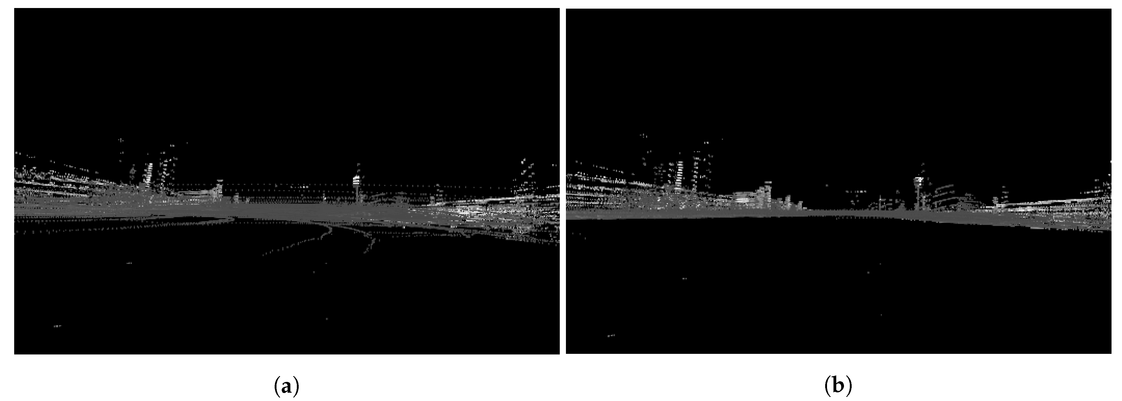
Figure 2.
Comparison of the effective range of LiDAR accumulation in a (b) spatial region as described
in Section 3.1.1, compared to a single LiDAR scan (a). In (b), data are not just accumulated in a temporal window around the current radar capture time. Rather, the initial set of LiDAR scans (before downsampling and pruning, etc.) which are fed into the automatic labelling method of Section 3.2 are taken at every pose within a certain range of the vehicle (centre of the scan) in an effort to populate the entire radar sensing horizon with sparse LiDAR measurements. We use multiple traversals of the environment to generalise the learning procedure to the lifetime of operation of the survey vehicle and maximise the capture overlap of LiDAR and radar. Some procedures for cleaning up of this dense accumulated point cloud are required and are dealt with in Section 3.1.2, Section 3.1.3, Section 3.1.4 and Section 3.1.5. In this example, a (b)
spatial accumulation fills out the radar scan more satisfactorily than a (a) temporal accumulation.

Figure 3.
A comparison of the accumulated point clouds (a) before and (b) after spatial downsampling as described in Section 3.1.2. Basically, a new LiDAR scan is added to the accumulated dense point cloud every time the vehicle moves 10m from its last location. As a result, a sparser and less erroneous point cloud is produced. This step is primarily aimed at mitigating extreme density of points for calculating traversability (c.f. Section 3.2) while still maintaining the extended LiDAR sensing horizon (out to the radar horizon) as per Section 3.1.1.

Figure 4.
Comparison of an accumulated point cloud (a) before and (b) after the removal of repeated traversals as described in Section 3.1.3. The intuition behind this step is that natural environments, particularly those in an urban setting, are time variant. Different obstacles are likely present at different times of traversal, leading to the superposition of false phantom obstacles with the obstacles present at the time of capture of the radar scan. Both of the above effects mean any computed traversability labels (c.f. Section 3.2) will be a poor representation of the environment as seen by the radar scan and thus provide poor supervision. In this example, the vertical road segment becomes sparser and better aligned.

Figure 5.
A cross-section of road in a LiDAR point cloud (a) before and (b) after standard iterative closest point (ICP) refinement as described in Section 3.1.4. A GPU-accelerated iterative closest point (ICP) algorithm is used in this work, which is modified to include a maximum correspondence distance threshold. Only the Neural Network (NN) points with relative displacements less than this threshold proceed to the singular value decomposition (SVD) step used to evaluate the least squares optimal rigid body transformation. The resulting registration is more robust to partial overlap of point clouds. Rather than applying iterative closest point (ICP) to point clouds of full density, random sampling of a subset of 15,000 points is applied to both the source and destination point clouds to reduce the computational load. Figure 6 describes an improved segmentation-based iterative closest point (ICP) which completes our implementation of this step of the accumulation of the dense point cloud in the radar scanning horizon.

Figure 6.
A comparison of the output of the traversability labelling pipeline with the (a) naïve registration approach and the (b) segmentation based approach as described in Section 3.1.4. This approach handles the registration of each traversal separately by identifying where each registered segment joins all other segments via a spatial nearest neighbour search. Segment boundaries are imposed anywhere the displacement between timestamp-consecutive poses is greater than a threshold value. A value of 15mis found to work well for this threshold. In this example, the segmentation-based approach shows superior performance at junctions.

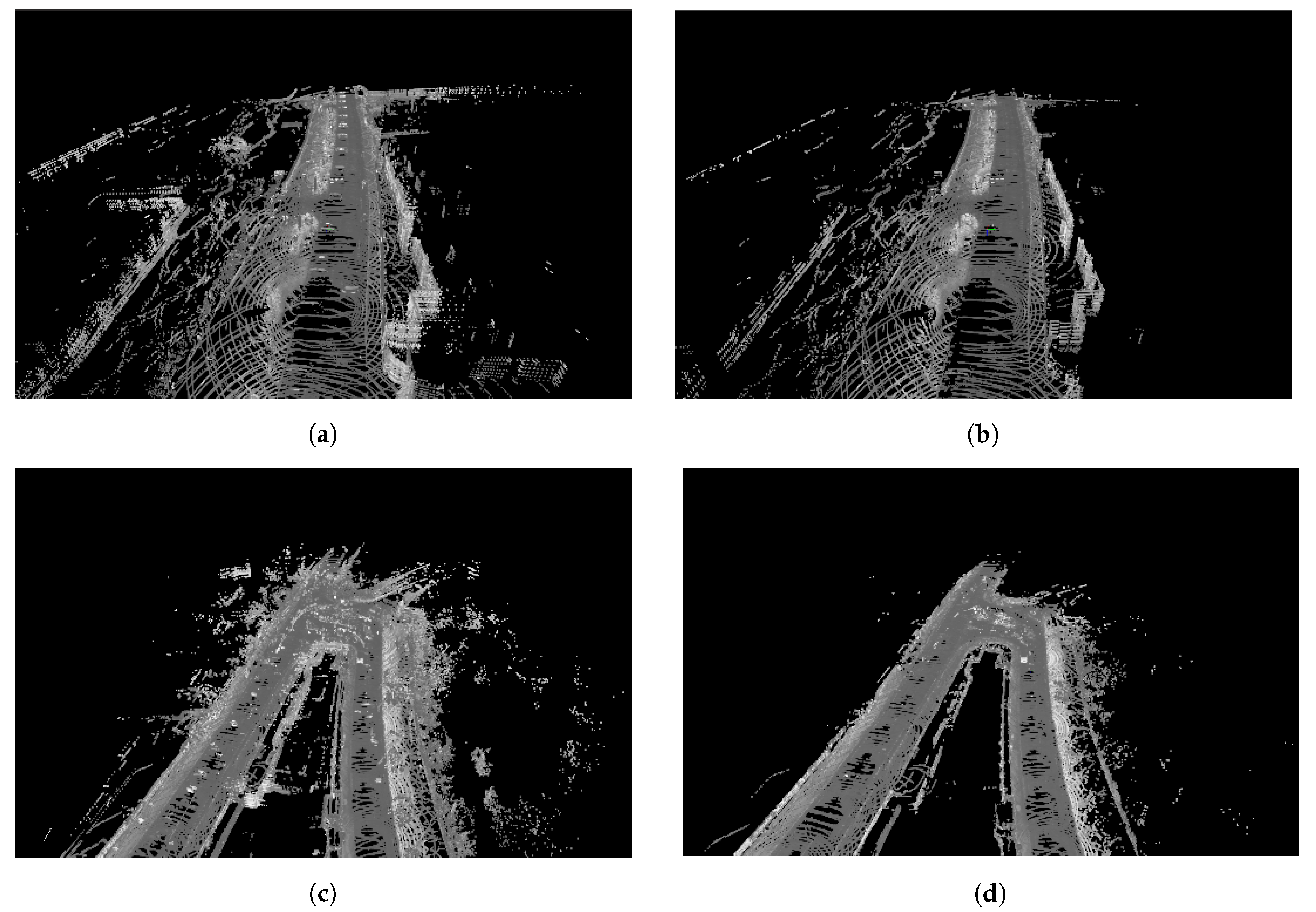
Figure 7.
A comparison of accumulated LiDAR point clouds (a,c) before (left) and (b,d) after (right) removal of duplicate dynamic obstacles from a dense point cloud accumulated over examples take from (a,c) straight and (b,d) curved road sections. In both cases duplicate cars are removed from the road and there is a reduction in erroneous points.

Figure 8.
Membership functions for fuzzy sets that describe gradient, roughness, height range and traversability.
Figure 8.
Membership functions for fuzzy sets that describe gradient, roughness, height range and traversability.

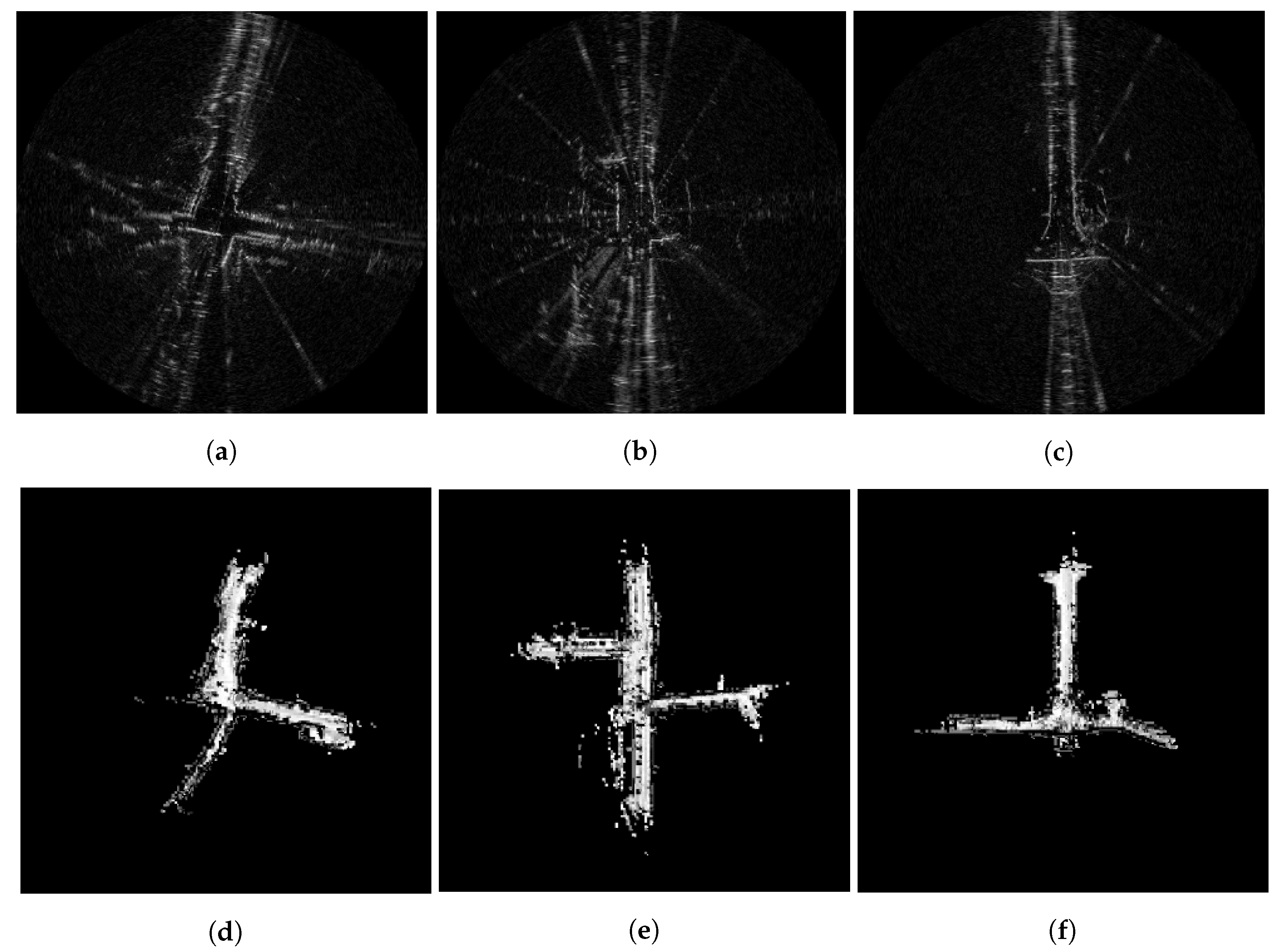
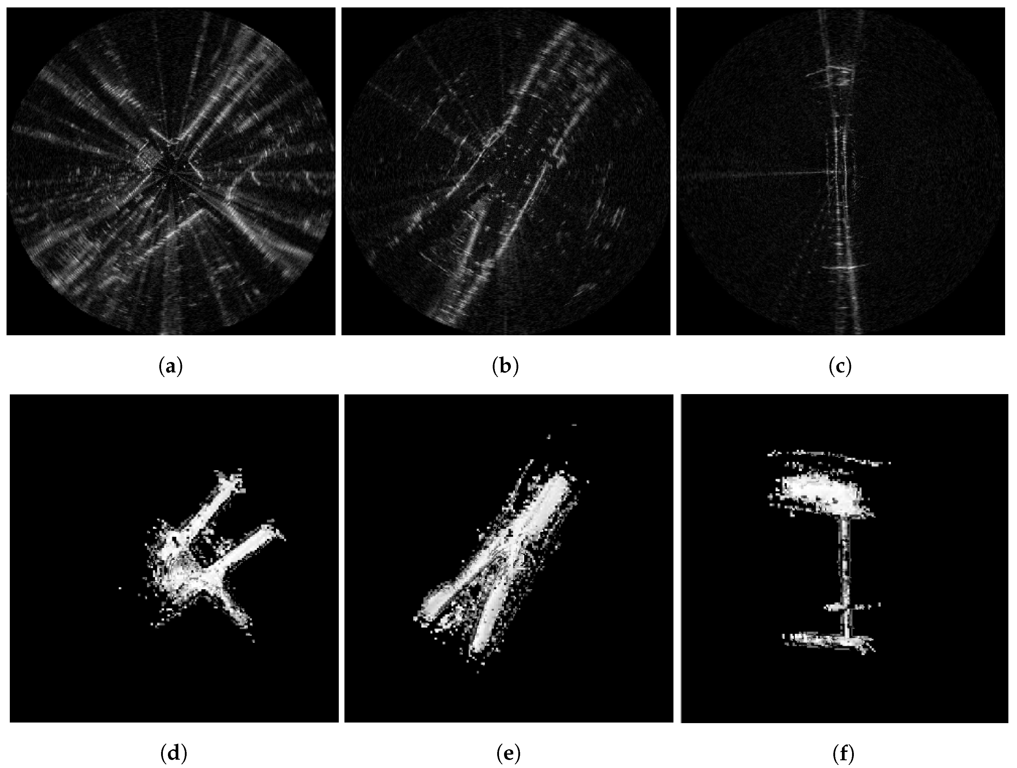
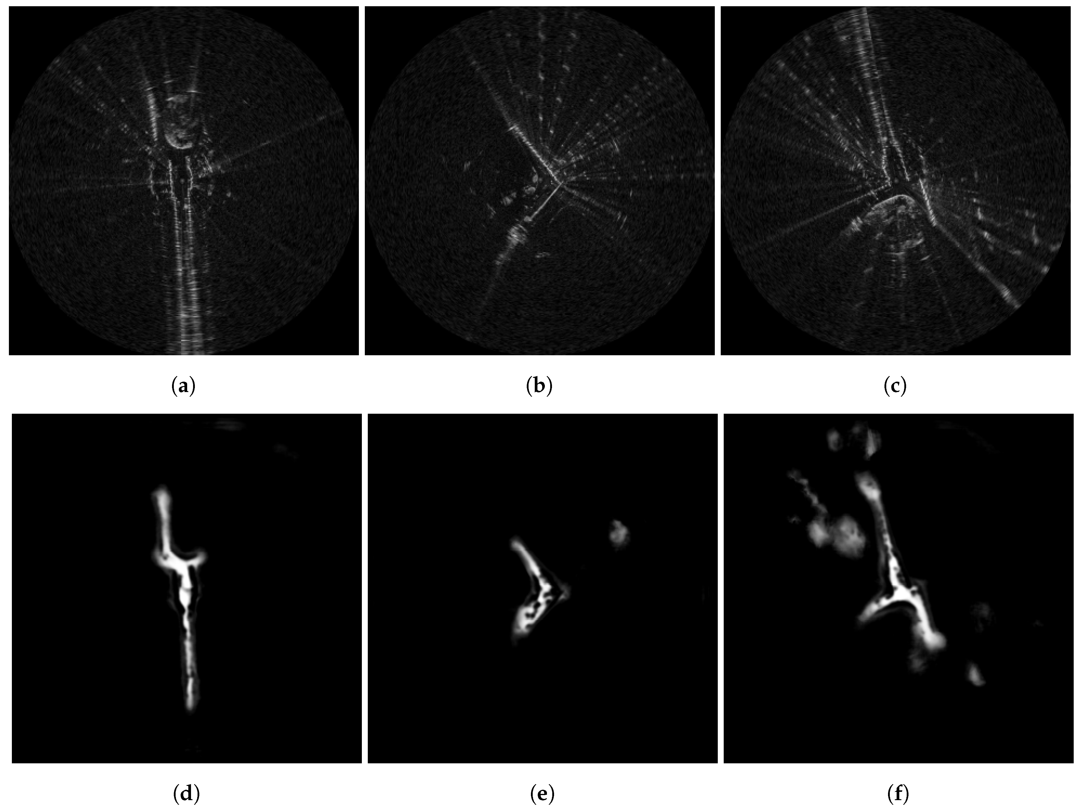
Figure 9.
Radar scans (top) and corresponding traversability labels (bottom) captured and computed in three places where the road layout features junctions. In the left example (a,d), the autonomous vehicle (AV) survey vehicle travels south-to-north along the vertically running stretch of road and sparse LiDAR measurements are accumulated along the resulting pose chain. In the middle example (b,e), the two east-to-west junctions are visited at later times and the pose chain consists of loop closures which allow the LiDAR measurements from later times to feature in the current volume. In the right example (c,f), however, there is never any revisit to the south road section. As such, no LiDAR points are accumulated there.

Figure 10.
Radar scans (a–c) and corresponding traversability labels (d–f) captured and computed in three places featuring mixed urban canyon and open areas. Notice in these examples that radar sensory artefacts (e.g., the radiating saturation lines left, speckle noise middle, and duplicate south-to-north road boundary) are not featured in the dense accumulated point cloud. We thus expect the Neural Network (NN) model in Section 3.3 to learn a characterisation of the radar scan which is more intelligent than simply applying thresholds on the power (dB) return. The results shown in our first tested model (c.f. Section 6.1) confirm this.

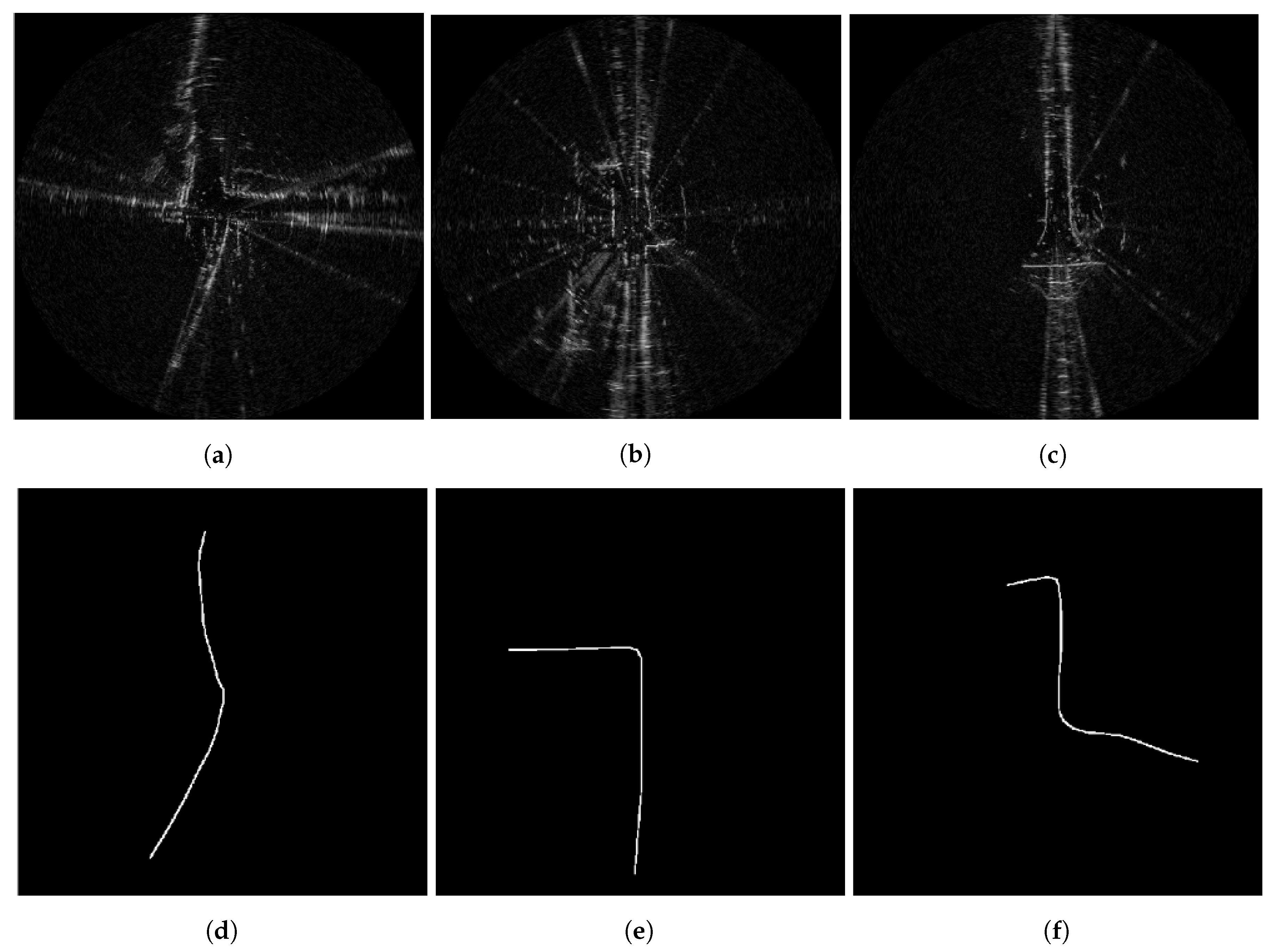
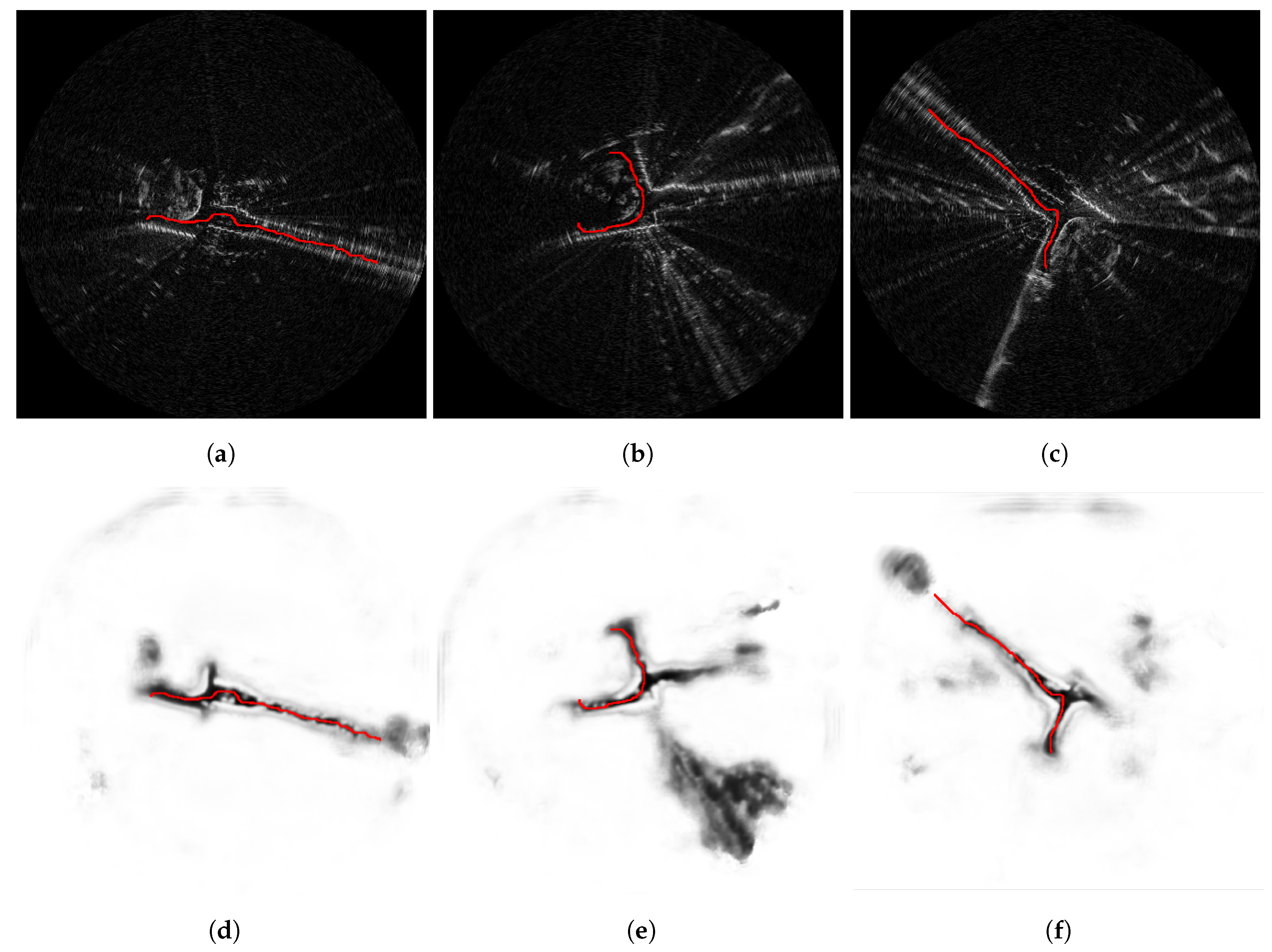
Figure 11.
Radar scans and corresponding route labels at junctions, prepared as per Section 4.1. In (a,d), the vehicle veers left while travelling south-to-north. In (b,e), the vehicle takes a left turn while travelling north. In (c,f), the vehicle takes a right turn shortly after taking a left turn. All of these driving behaviours (and others) are possible in various scenes typically sensed by the radar at long range, and we expect that the Neural Network (NN) model designed in Section 4.2 below will generalise beyond simply learning the demonstrations shown to it during training. We indicate this experimentally in Section 6.2.

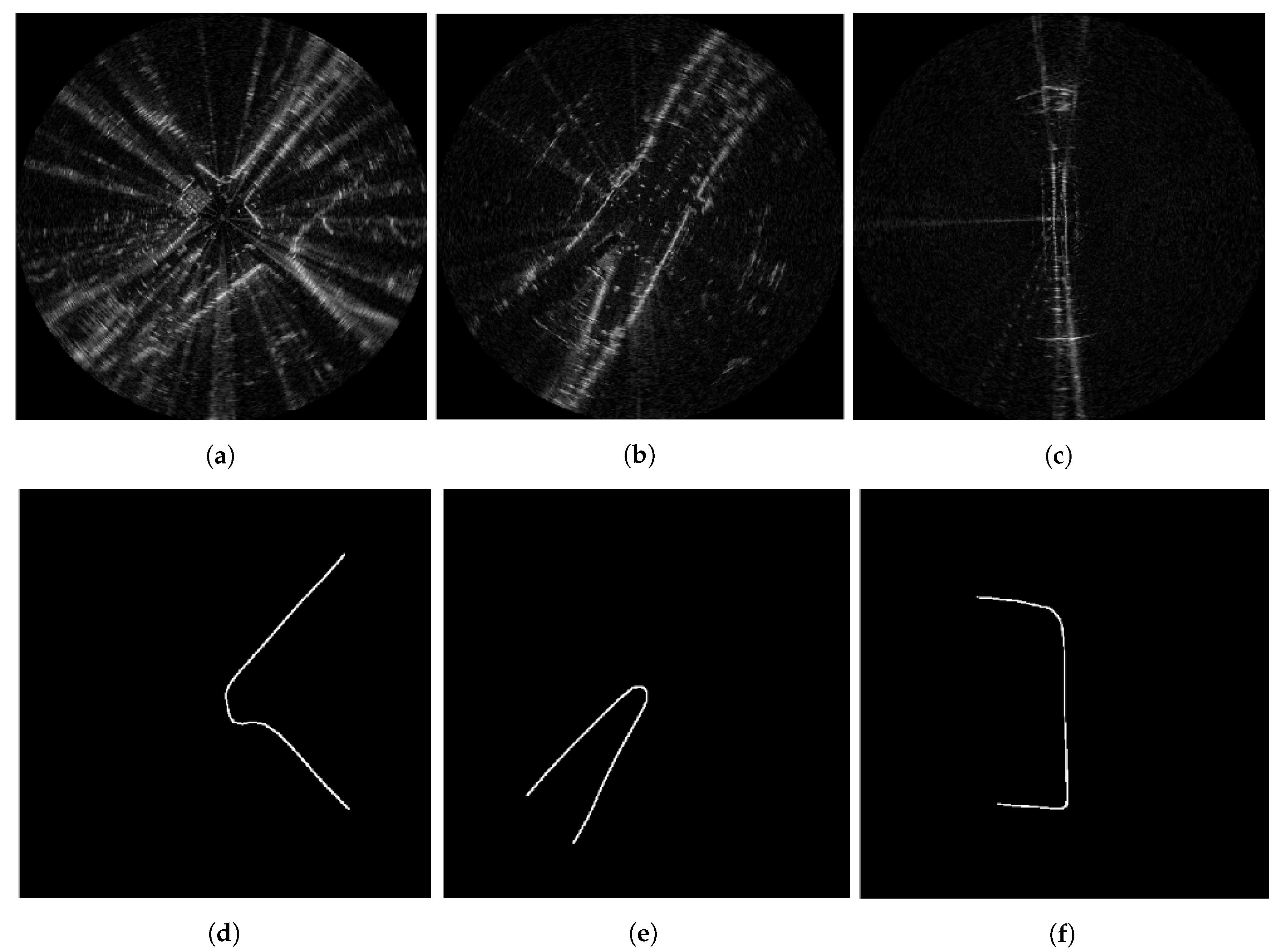
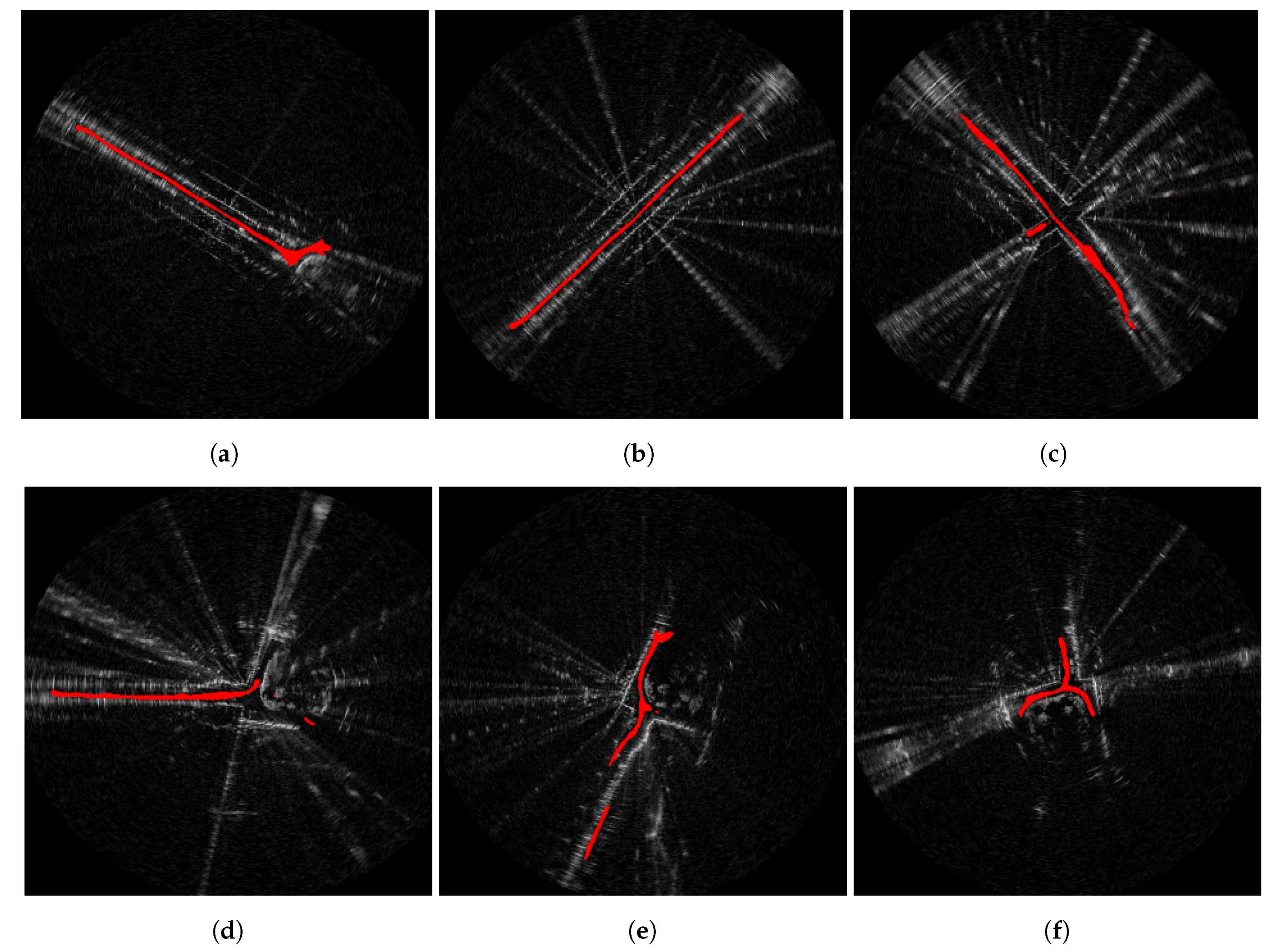
Figure 12.
Radar scans and corresponding route labels where open areas are present, prepared as per Section 4.1. In (a,d), the test vehicle travels from one narrow street (south-east) to another narrow street (north-east) via an open area. In (b,e), the vehicle travels around an open area only. In (c,f), the vehicle travels from one open area (south) to another open area (north) via a narrow street.

Figure 13.
(a) The autonomous-capable Nissan Leaf data collection platform as equipped in Section 5.1 for the dataset described in Section 5.2 and (b) the 10km route driven in the Oxford Radar Robotcar Dataset. The route is partitioned into training, validation and test data. These are coloured as blue, red, and purple respectively.

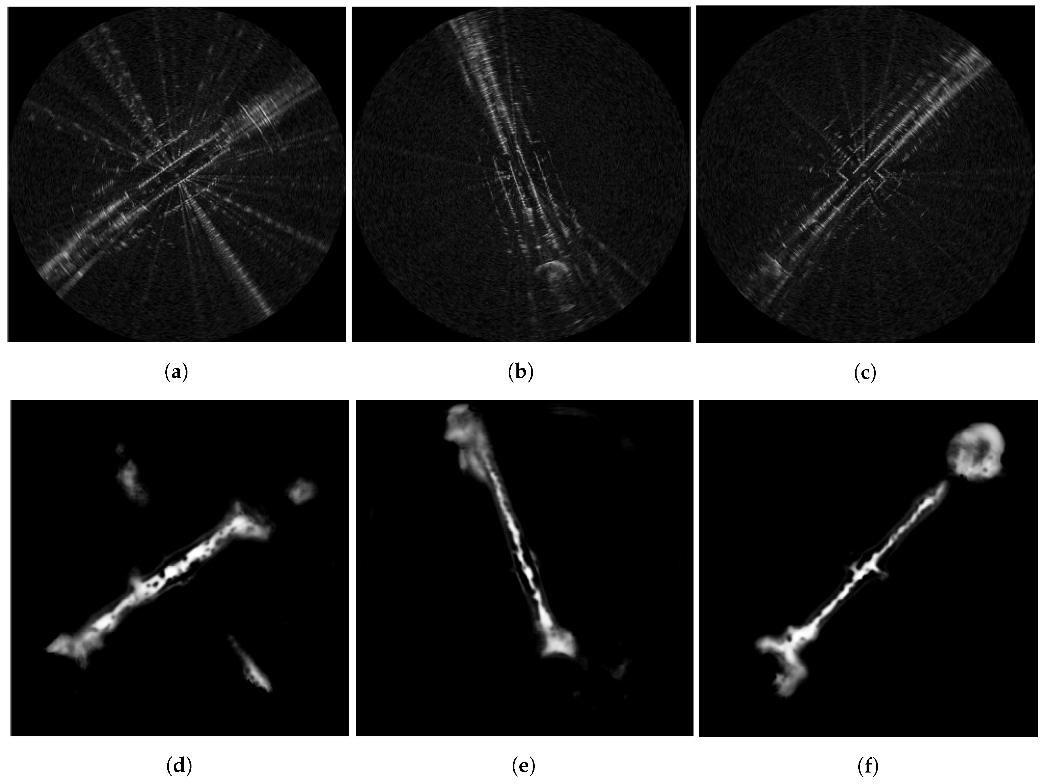
Figure 14.
Traversability predictions on straight road segments in the presence of radar artefacts as described in Section 6.1. In (a,d), saturation lines (radiating from the vehile location at the centre of the scans). In (b,e), ringing effects cause the appearance of duplicate roads. In (c,f), occlusion effects obscure the perception of the environment (top right open area). All of these effects present no significant issue to the traversability model.

Figure 15.
Traversability predictions for radar scans in a challenging urban environment as described in Section 6.1. These radar scans are taken in close proximity to one another, as the vehicle turns in a tight circle. Large areas of the radar scans are occluded by an elevated central roundabout, resulting in unusual road geometry. In (a,d), the vehicle approaches the turn. Here, the urban canyon behind the vehicle is understood by the model to be traversable, as is the way (left) into the turn. In (b,e), the vehicle is mid-way around the turn. Here, the road ahead and behind of the vehicle is entirely made up of turn, which is understood to be traversable. The model no longer sees the urban canyon due to the occlusion of the central feature. In (c,f), the vehicle is exiting the turn and reentering a straight urban canyon. Here, the model understands that the urban canyon as well as the original turn around the central feature are traversable.

Figure 16.
A sample of maximally traversable routes evaluated using the A* graph search algorithm. (a–c) show the optimally traversable routes (red) projected onto the corresponding FMCW radar scans. (d–f) represent the vertex weighted graphs which are computed from the inferred traversability maps and on which the minimum cost routes between the start and destination points are projected. The routes evaluated using the A* algorithm are found to be robust for a wide range of radar scans in the test data, including those with significant artefacts present. They reliably navigate around obstacles while exhibiting paths that are direct, implying good performance from the traversability prediction network. The smoothness of the inferred paths leaves something to be desired; however, an issue which is resolved by the multi-task learned model in Section 6.2.

Figure 17.
A sample of route proposal cases for straight road segments (top row) and junctions (bottom row). The model deployed here was trained only using route labels (c.f. in the learned objectives of Section 4.2.2). In (a), the vehicle track width of 1.4m is not totally maintained by the model—see Figure 18 for an improvement to this. In (b), no turns off of the current route are perceived or proposed. The situation in (c), in contrast, is understood by the model as feasible to continue driving straight or turn left off of the current route. In (d), a slight left past a non-traversable feature is yielded as the traversable route. In (e), there are some gaps in the traversable route proposed by the network. These drop-outs in predictions are resolved in Figure 18. In (f), the model understands that a left or right turn after the current path terminates is feasible. Please see Section 6.2 for further discussion.

Figure 18.
A sample of routes proposed for several different urban settings. The model deployed here was trained using traversability maps as well as route labels (c.f. and in the learned objectives of Section 4.2.2). The proposed routes are seen to outperform those presented in Figure 17. As compared to Figure 18a, the proposed vehicle track of (a), is more consistent in width. In (a,e) an obstacle ahead of the vehicles trajectory is understood to be non-traversable, and routes to the left or right of this feature are proposed. In (b), the vehicle drives along a narrow urban canyon, and no turns off of this route are seen as possible. In (c), the model admits for a left or right turn at the end of a narrow urban canyon. In (d), the model understands that a right turn off of the current path is feasible. In (f), the vehicle is circumnavigating a walled off park, and the turn out of this urban feature is not yet visible. Please see Section 6.2 for further discussion.

Figure 19.
Examples of planned routes through various environments. Left (a,c,e,g) are shown the plans generated by A* planning through the traversability map. Right (b,d,f,h) are shown the plans generated by Medial Axis Transform (MAT) or “skeletonization” of the routes inferred by the model trained using traversability maps and route labels in conjunction. In all cases, the routes yielded by the A* approach do not exhibit the same level of “smoothness” as those shown right, which better reflect the kinematic capabilities of the vehicle.

Publisher’s Note: MDPI stays neutral with regard to jurisdictional claims in published maps and institutional affiliations. |
© 2020 by the authors. Licensee MDPI, Basel, Switzerland. This article is an open access article distributed under the terms and conditions of the Creative Commons Attribution (CC BY) license (http://creativecommons.org/licenses/by/4.0/).
Share and Cite
MDPI and ACS Style
Broome, M.; Gadd, M.; De Martini, D.; Newman, P. On the Road: Route Proposal from Radar Self-Supervised by Fuzzy LiDAR Traversability. AI 2020, 1, 558-585. https://doi.org/10.3390/ai1040033
AMA Style
Broome M, Gadd M, De Martini D, Newman P. On the Road: Route Proposal from Radar Self-Supervised by Fuzzy LiDAR Traversability. AI. 2020; 1(4):558-585. https://doi.org/10.3390/ai1040033
Chicago/Turabian StyleBroome, Michael, Matthew Gadd, Daniele De Martini, and Paul Newman. 2020. "On the Road: Route Proposal from Radar Self-Supervised by Fuzzy LiDAR Traversability" AI 1, no. 4: 558-585. https://doi.org/10.3390/ai1040033