Mapping Cropland Intensification in Ecuador through Spectral Analysis of MODIS NDVI Time Series

Abstract

Multiple cropping systems constitute an essential agricultural practice that will ensure food security within the increasing demand of basic cereals as a consequence of global population growth and climate change effects. In this regard, there is a need to develop new methodologies to adequately monitor cropland intensification. The main objective of this research was to assess cropland intensification by means of spectral analysis of MODIS NDVI time series in a high cloudiness tropical area such as Ecuador. A surface of 89,225 ha of the main staple crops in this country, which are rice and maize crops, was monitored to assess the evolution of the number of crop cycles. The 20-year period of NDVI time series was used to calculate the periodograms across four subperiods (2001–2005, 2006–2010, 2011–2015, 2016–2020). The maximum ordinate value of each periodogram was used as an indicator of the number of growing crop cycles per year identifying single-, double-, and triple-cropping systems in each subperiod. Cropland intensification was assessed by comparing the cropping system between the subperiods. Results reveal that more than half of the studied croplands experienced changes in the cropping systems, and 40% showed positive trends in terms of the number of growing crop cycles, being principally located near the main rivers where irrigation facilitates crop development during the dry season. Therefore, the area under single cropping decreased from over 60,000 ha in the first subperiod to less than 50,000 ha in the last two subperiods. The cropland surface subjected to multi-cropping practices increased during the second decade of the study period, with a double-cropping system being more widely used than growing three crops per year, reaching surfaces of 24,400 ha and 10,450 ha in the last subperiod, respectively. The robust results obtained in this research show the great potential of the periodogram approach for the discrimination of cropping systems and for mapping intensification areas in tropical regions where dealing with noisy remote sensing time series as a consequence of high cloudiness is a great challenge.

1. Introduction

In the current context of climate change and food scarcity, agricultural intensification by growing two or more crops per year in the same field [1] is a common practice to increase crop yield. Production of rice and maize, the cereals most cultivated around the world, has experienced an increment of approximately 2.5% and 21.8% during the last decade, with an estimated global harvested area of 164 and 201 million hectares in 2020, respectively [2]. This positive trend of food consumption, along with climate change effects on crop productivity, is increasing food insecurity [3]. It is expected that an increase of 70–110% in food production will be necessary to feed approximately 9 billion people by 2050, which means reaching about 3 billion tons of annual cereal production [4,5,6]. In this context, the United Nations General Assembly formulated the second Sustainable Development Goal (SDG) as part of the Agenda 2030 with the aim to reach zero hunger while maintaining agricultural and environmental sustainability [7].

The intensification and expansion of agricultural areas are the two main strategies to cope with the lack of grain yield [7,8]. Farmland expansion is limited in many regions by environmental factors, so that the intensification of existing agricultural areas arises as a suitable practice to mitigate food scarcity frequently with serious environmental consequences, such as water scarcity, soil contamination, increase in greenhouse gases emissions, or biodiversity loss [9,10,11,12]. Multiple cropping practices show considerable spatial and temporal variability at a global scale depending mainly on socioeconomic and climate factors and being especially widespread across tropical areas [13,14,15,16]. From 2000 to 2010, most of the North American and European countries showed a stable cropland area with a moderate cropland intensification whereas the most prominent intensification was found in China, India, and in tropical areas of southeast Asia, west Africa (e.g., Ghana and Liberia), and South America [17], probably due to the improvement of technology during this decade. Specifically in Ecuador, the intensification process has been a relevant measure to increase productivity by developing new irrigation infrastructures [18].

To assist decision-makers in assessing production and formulating appropriate agricultural policies that achieve a balance between agricultural intensification and environmental conservation, it is necessary to develop operational methodologies to provide spatial and temporal information about multiple cropping practices. Traditionally, the most used methods for collecting information about the estimation of cropland areas and cropping intensity have been agricultural census statistics together with land surveys. However, these approaches are time-consuming, expensive, and do not provide the information in a timely manner [13,19].

In the last decades, remote sensing techniques have been demonstrated to be an effective tool for monitoring agricultural areas, providing periodic information about Earth’s surface at different time scales. The Group on Earth Observations Global Agricultural Monitoring Initiative [20] encourages the development of new methodologies using remote sensing data to continue improving crop monitoring, contributing to market transparency and food security, specifically those that can be applied across different environments to monitor staple crops such as rice and maize [21]. The use of vegetation indices from moderate resolution imaging spectroradiometer (MODIS) has proved to be effective for crop monitoring at large scales [22,23,24,25,26] because of the combination of moderate spatial resolution, high temporal frequency, and length of the time series [27,28,29,30,31,32].

The phenological evolution of crops makes it possible to map cultivated fields and assess cultivation intensity by evaluating the number of annual peaks in vegetation indices time series. For instance, Estel et al. [33] derived single- and double-cropping maps in Europe by counting the number of NDVI peaks using TIMESAT based on the amplitude ratio between the primary and the secondary peaks. Ding et al. [34] identified a bimodal pattern in China establishing a NDVI minimum threshold value and a time lapse of two months between two consecutive peaks. Sakamoto et al. [32] and Kontgis, Schneider, and Ozdogan [35] identified the number of rice crops per year in Mekong basin by the local maximal points of EVI higher than 0.4. In addition, Guo et al. [7] and Liu et al. [36] used the NDVI annual peaks with values higher than 0.5 as part of their methodology to identify a double-cropping system.

However, in tropical areas, these methodologies are limited where the cloud coverage is extremely frequent and precipitation very high. In these regions, the amount of noise in the vegetation indexes time series makes it difficult to extract significant information content when applying phenometric methods in which threshold values need to be set [37,38]. Thus, this approach strongly depends on time series filtering being difficult to quantitatively evaluate the best algorithm for every phase of crop growth [27], affecting the results depending on the algorithm used [39].

Statistical time series analysis, based on the entire time series, makes it possible to diminish the impact of the noise in the time series and enhance the relevant information to quantitatively assess cropland dynamics not using specific threshold values. Particularly, the spectral analysis makes it possible to decompose a time series into sinusoidal components and explain the periodicity patterns existing in the data [40,41]. This methodology is highly appropriate to explain vegetation dynamics [42] because of the significance of their seasonal component.

The availability of earth observation (EO) time series provides an excellent opportunity to apply this approach, making it possible to quantitatively elucidate intra and interannual vegetation dynamics enriched by the consistency provided by the spatial component [43,44,45]. In this context, Azzali and Menenti [46] used the fast Fourier transform (FFT) to represent vegetation phenology based on the AVHRR NDVI ten-year time series. In this work, they were able to map homogeneous land units in terms of leaf phenology based on amplitude and phase images. Other authors have used spectral analysis to uncover vegetation cycles in natural vegetation and crops [47,48,49]. Mingwei et al. [50] and Canisius et al. [51] identified double-cropping systems through a Fourier analysis based on MODIS and NOAA NDVI time series, respectively.

In spite of the promising results, this methodology is not frequently used in EO, maybe because of the difficulty to represent periodicities in the spatial domain (territory). In this context, the periodogram is an operational tool that allows us to quantitatively estimate the proportion of variability explained by each of the cycles with respect to the total amount of variability in the time series [41,52]. This makes it possible to map intra-annual and pluri-annual cycles based on the percentage of variability accounted for by each of the time series periodicities. Huesca et al. [53] used information from the periodogram parameters to estimate the seasonality of fire risk in three bioclimatic regions in Spain. Based on periodogram ordinates, Recuero et al. [54] generated maps of NDVI amplitude as well as the number of intra-annual cycles and their stability from AVHRR NDVI 35-year time series at a global level. As the length of the time series increases, the reliability of spectral analysis also improves [42], providing parameters with higher significance. Our hypothesis is that it is possible to assess land use changes throughout long time periods by assessing differences between subperiods based on their dynamics.

The aim of this study is to assess and map the evolution of cropping intensity (number of crops per year) throughout the period 2001–2020 in four 5-year subperiods in the tropical region of Ecuador. Specifically, we propose to use periodogram analysis of NDVI time series to determine the number of intra-annual crop growth cycles within each 5-year period in the study area, dealing with the high noise content of the time series.

2. Materials and Methods

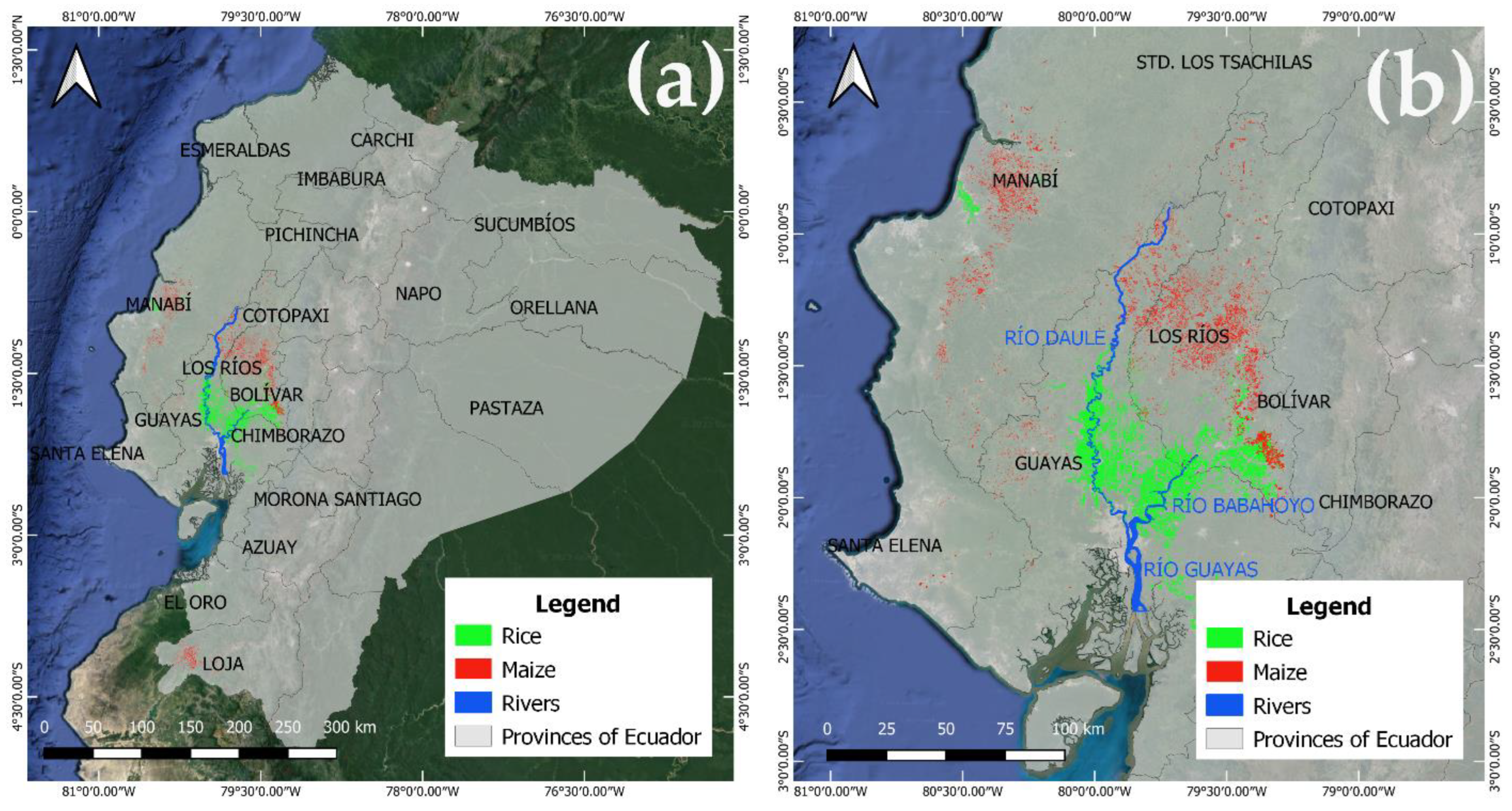
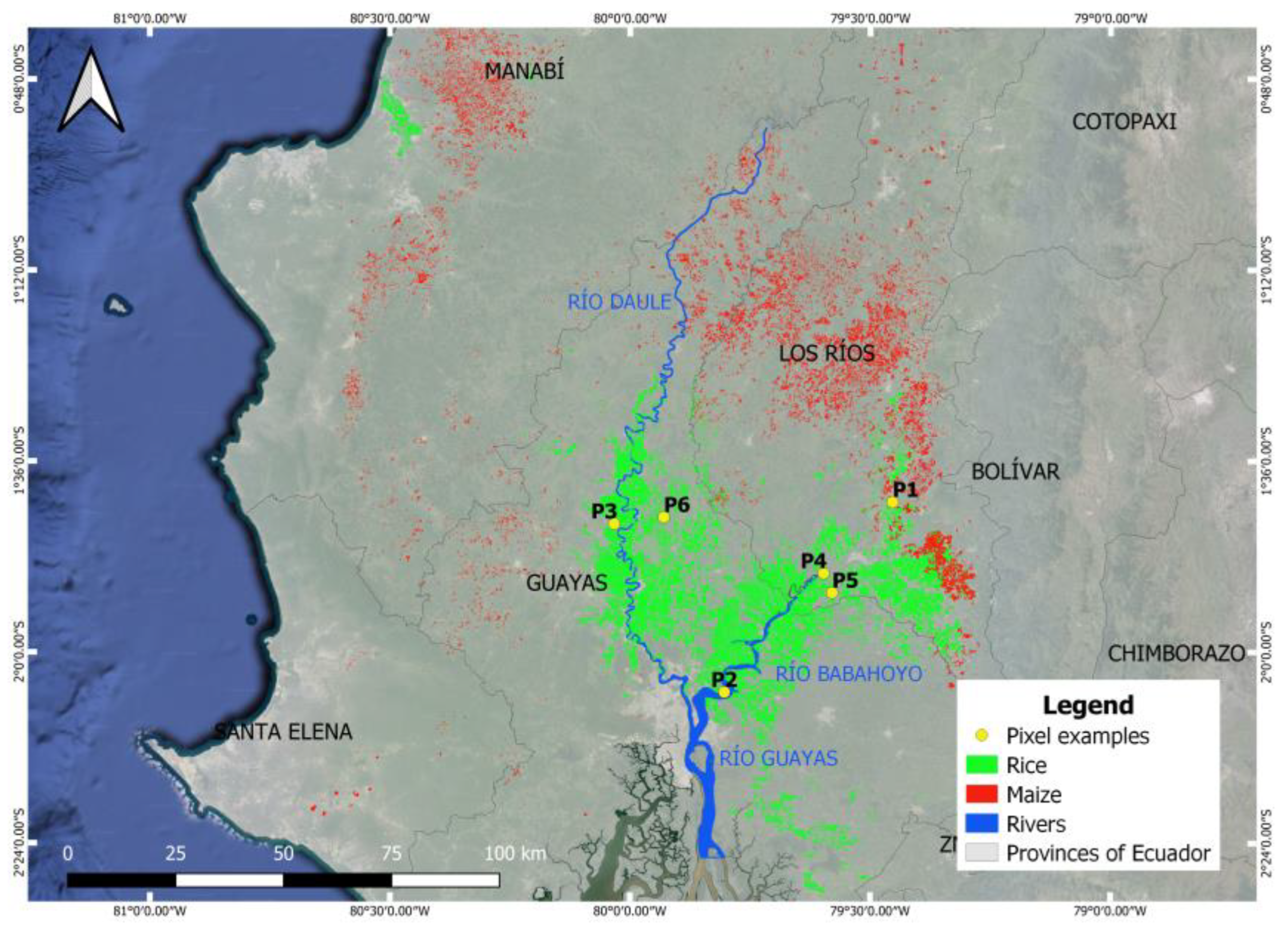
2.1. Study Area

The study area includes rice and maize cultivated areas in mainland Ecuador, a country located in northwestern South America, bordered to the north by Colombia, to the east and south by Peru, and to the west by the Pacific Ocean. They constitute the main staple crops cultivated in this region, occupying approximately 479,420 ha, 21% of the areas destined for agricultural use [55]. These crops are mainly cultivated in the provinces of Guayas, Los Rios, Manabi, and Santa Elena in the Midwest part of the country (Table 1). Their spatial distribution for 2020 can be seen in Figure 1, where rice and maize are displayed in green and red, respectively. These crops constitute the main staple food for the population of Ecuador, which experienced an increment of approximately 38% since 2001, reaching 17.6 million people in 2020 [2].

According to the Köppen climate classification, the climate in these areas is tropical with a dry season (Aw) between June and November. The mean annual temperature ranges between 20 °C and 26 °C and the mean annual precipitation from 1200 mm and 2000 mm [56,57]. This region is characterized by high cloudiness with a mean annual of 7 oktas on a scale ranging from 1 (minimum cloudiness) to 8 (maximum cloudiness) [58]. Daule and Babahoyo rivers cross the study area, increasing water availability for growing. crops.

Figure 1. Location of mainland Ecuador (a) and zoom to the rice and maize cultivated areas in mainland Ecuador in 2020 represented in green and red, respectively (b).

Figure 1. Location of mainland Ecuador (a) and zoom to the rice and maize cultivated areas in mainland Ecuador in 2020 represented in green and red, respectively (b).

Table 1. The provinces with the largest harvested area (ha) and production (t) in 2020 in Ecuador [59].

Rice			Maize
Province	Harvested Surface (ha)	Production (t)	Province	Harvested Surface (ha)	Production (t)
Guayas	216,853	1,123,754	Los Ríos	101,258	588,091
Los Ríos	76,733	344,946	Manabí	78,388	379,858
Manabí	6,747	32,527	Santa Elena	4,646	23,305

Table 1. The provinces with the largest harvested area (ha) and production (t) in 2020 in Ecuador [59].

Rice			Maize
Province	Harvested Surface (ha)	Production (t)	Province	Harvested Surface (ha)	Production (t)
Guayas	216,853	1,123,754	Los Ríos	101,258	588,091
Los Ríos	76,733	344,946	Manabí	78,388	379,858
Manabí	6,747	32,527	Santa Elena	4,646	23,305

2.2. Data Sources

2.2.1. Remote Sensing Data

MODIS data were chosen because of the daily frequency of the Earth observations, which allows us to deal with the high cloudiness in tropical areas such as Ecuador. In addition, the availability of more than 20 years of observations provides robustness to the results.

The MODIS MOD09A1 version 6 product [60], which consists of 8-day composites at 500 m spatial resolution, was acquired for the period 2001–2020 from the NASA website (https://lpdaac.usgs.gov, accessed on 12 September 2022) and reprojected to UTM zone 17. This dataset, with a total of 920 images, contains information in seven spectral bands centered at 450 nm (blue), 555 nm (green), 645 nm (red), 860 nm (NIR), 1240 nm (SWIR1), 1640 nm (SWIR2), and 2130 nm (SWIR3).

2.2.2. Estimations of Sown Surfaces

The estimations of sown surfaces of rice and yellow dent maize for the periods 2014–2015 and 2019–2020 were provided in shapefile format by the Ministry of Agriculture and Livestock of Ecuador (MAG, from the acronym in Spanish) [59] and were considered as representative for the third and the fourth subperiods. This information was used to extract pixels with at least 80% cultivation of one of these crops, resulting in a total of 3569 pixels, equivalent to 89,225 hectares, which represents approximately 20% of the cropland area dedicated to growing these two crops.

These data consist of yearly information about the sown surface during three monitoring periods for rice: December–March, April–July, and August–November and during two periods for maize, which are December–May and June–November (

Table 2. Number and duration of the phenological cycles of rice and maize.

Crop	Months
	Dec.	Jan.	Feb.	Mar.	Apr.	May	Jun.	Jul.	Aug.	Sep.	Oct.	Nov.
Rice
Maize

). Farmers usually sow these cereals in the rainy season, that is, between December and May. Thus, 25–30% of the total sown area with rice occurs during the first period, 45–50% during the second period, and 30% in the third period [59]. Farmers rarely sow a third time [61]. Regarding to maize, 80% of the sown surface occurs in the first period and 20% during the second period [59]. Most of the crops sown during the dry period are subjected to irrigation systems, flood irrigation when cultivating rice, and sprinkler irrigation for maize crops. The use of a different irrigation system, combined with the lack of legal obligation to perform crop rotations, makes it challenging to implement crop rotation using rice and maize alternatively. However, maize–soy crop rotation has been observed in some areas [59].

The methodology that MAG employs to develop this cartography is processing and visual interpretation of high-resolution satellite imagery (e.g., Sentinel-2, RapidEye, PlanetScope, Landsat-8 and 9) with the support of field data and orthophotos among other ancillary information [59].

2.3. NDVI Time Series Generation

The 20-year normalized difference vegetation index (NDVI) time series was calculated from red (${\mathsf{\rho }}_{\mathrm{R}\mathrm{E}\mathrm{D}}$) and near-infrared (${\mathsf{\rho }}_{\mathrm{N}\mathrm{I}\mathrm{R}}$) surface reflectance time series as follows [62]:

$$\mathrm{N}\mathrm{D}\mathrm{V}\mathrm{I}=\frac{{\mathsf{\rho }}_{\mathrm{N}\mathrm{I}\mathrm{R}}-{\mathsf{\rho }}_{\mathrm{R}\mathrm{E}\mathrm{D}}}{{\mathsf{\rho }}_{\mathrm{N}\mathrm{I}\mathrm{R}}+{\mathsf{\rho }}_{\mathrm{R}\mathrm{E}\mathrm{D}}}$$

(1)

where ${\mathsf{\rho }}_{\mathrm{R}\mathrm{E}\mathrm{D}}$ and ${\mathsf{\rho }}_{\mathrm{N}\mathrm{I}\mathrm{R}}$ are the reflectance values at red and near-infrared spectral bands, respectively.

The NDVI time series consists of 920 values (i.e., 46 observations per year). These time series were divided into four equal subperiods with 230 observations each: (1) 2001–2005; (2) 2006–2010; (3) 2011–2015; and (4) 2016–2020.

NDVI time series for the entire period and subperiods were filtered in order to remove possible outliers due to high cloudiness. These abnormal values were identified as values falling outside the threshold of the mean plus/minus twice the standard deviation within a three-day observation period window. These values were replaced by the mean of the previous and subsequent observations. Then, a Savitzky–Golay filter [63] was applied to smooth the NDVI time series using the R package “prospectr” with a nine-date window and a degree of the smoothing polynomial of 2 [64].

2.4. Statistical Time Series Analysis

The assessment of NDVI time series seasonality was carried out by means of the periodogram, which allows us to identify the most relevant periodic components [41]. Periodogram is based on the classical mathematical theory of Fourier series in which the signal is decomposed into a series of sine and cosine waves at different frequencies called Fourier frequencies (f_i). Thus, the Fourier transform decomposition of the series X_t is shown in Equation (2) [65]:

$$X_t=a_0+\sum _{i=1}^m[a_i·\cos \left(2\pi f_{i}t\right)+b_i·\sin \left(2\pi f_{i}t\right)]+e_t$$

(2)

where

• X_t are the equally spaced time series data;
• t is the time subscript, t = 1, 2, …, n;
• n is the number of observations in the time series;
• a_i and b_i are the Fourier coefficients; I = 1, 2, …, m;
• m is the number of frequencies: m = n/2 if n is even; m = (n − 1)/2 if n is odd;
• f_i is the i-th Fourier frequency: f_i = i/n;
• a₀ is the mean term: a₀ = $\overline{x }$;

e_t: error term.

The importance of each frequency (f_i) for explaining the variance of time series is measured by the periodogram ordinate at that specific frequency (Equation (3)).

$$I\left(f_i\right)=\frac{n}{2}·({a_i}^2+{b_i}^2)$$

(3)

The periodogram is plotted as I(f_i) versus f_i for i = 1, 2, …, n/2 or (n − 1)/2 for time series with even and odd numbers of observations, respectively. NDVI periodograms for each subperiod have 115 frequencies (or periods). The most important periodicities are related to high values of I(f_i), indicating more variance explained by the frequency fi in the time series oscillation.

Before performing the Fourier decomposition, the series mean for all series was subtracted. This procedure prevents the distorting of a large first periodogram ordinate over the periodogram low frequencies [66] and can contribute to leakage reduction.

A rectangular window with constant weights was used to smooth the periodogram of the series (see Lags and Spectral windows in Jenkins and Watts, 1968, page 244 [67]) considering the criteria of resolution, stability, leakage, and smoothing proposed by Bloomfield (2000) [41].

In order to test the leakage effect, a pre-whitening procedure was performed by computing the first differences in a large subset of the series. Pre-whitening reduces the risk of leakage and allows the use of a more stable estimate with lower resolution [41]. The results show that the periodograms of the pre-whitened series are approximately the same as the periodograms of the series multiplied by |G(f)|², the power transfer function of the pre-whitening filter [41]. For this reason, the original series periodograms were used in this research.

The NDVI time series have a temporal frequency of 46 observations per year since the MOD09A1 imagery is made up of 8-day composites. Consequently, in the assessment of the main cropping system within a certain period, the most relevant periodic components are annual, 6 months, and 4 months (i.e., one, two, and three annual crop cycles) measured by the periodogram’s ordinate at periods 46, 23, and 15.3, respectively. The first two periodicities are integers, multiple of the number of observations (n = 230), while the third one, 15.3 is not. Therefore, it is expected to have some leakage problems from the third but not from the first two.

The Fisher’s kappa (FK) test [68] was used to evaluate the seasonality significance. The null hypothesis for this test is that time series is white noise, that is, a sequence of independent and random observations with zero mean. The considered critical value for rejecting the null hypothesis was 7.5 at the 5% significance level and for 115 ordinates. Spectral analysis was computed at series level by means of the Proc Spectra procedure of the SAS software (SAS 9.4 Software, SAS Institute Inc., Cary, NC, USA), whereas at image level (pixel), the R package “Genecycle” [69] was used for calculations over georeferenced images.

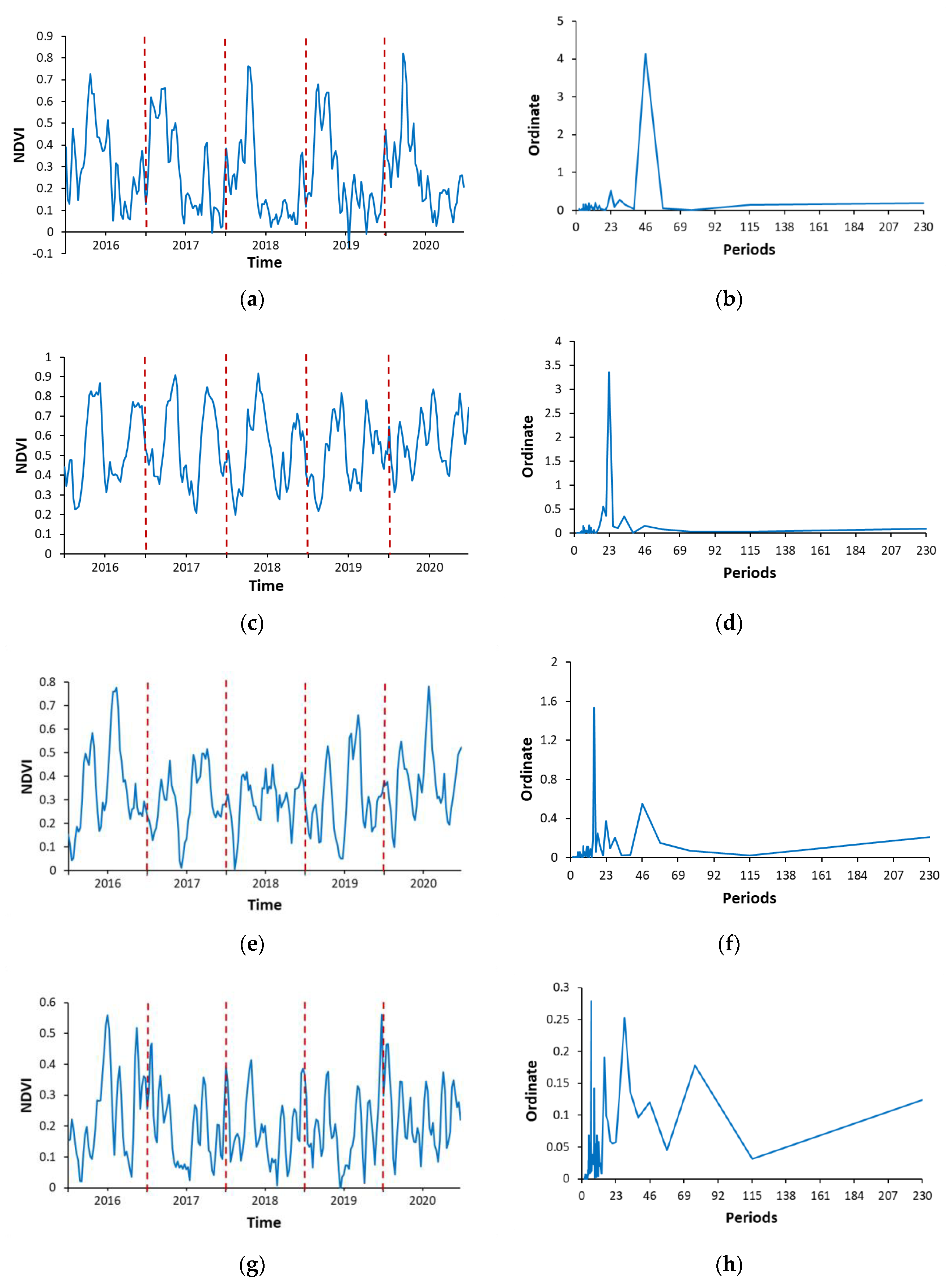
2.5. Determination of Cropping Intensity Based on NDVI Spectral Analysis

The dominant cropping system used within each subperiod was assessed according to the maximum ordinate of the periodogram. Therefore, single-, double-, and triple- cropping intensities were identified when the maximum ordinate is reached at the 46, 23, and 15.3 periods, respectively. Croplands with an undefined cropping pattern were found when the maximum occurs at a different period.

There are several important considerations about the characteristics of the NDVI time series in the study area that must be considered when evaluating periodicities by means of spectral analysis, because they may increase the uncertainty:

• NDVI time series with high noise content as a consequence of adverse climatic conditions with the presence of very dense clouds;
• The crop duration may be not exact each year making the identification of one, two, and three seasonal cycles more difficult;
• The changes in the cropping intensities within a certain subperiod may not allow the identification of the main pattern in this part of the study period.

Considering the cropland sown one, two, and three times, we calculated the equivalent sown surface by multiplying each surface pixel by one, two, and three, respectively.

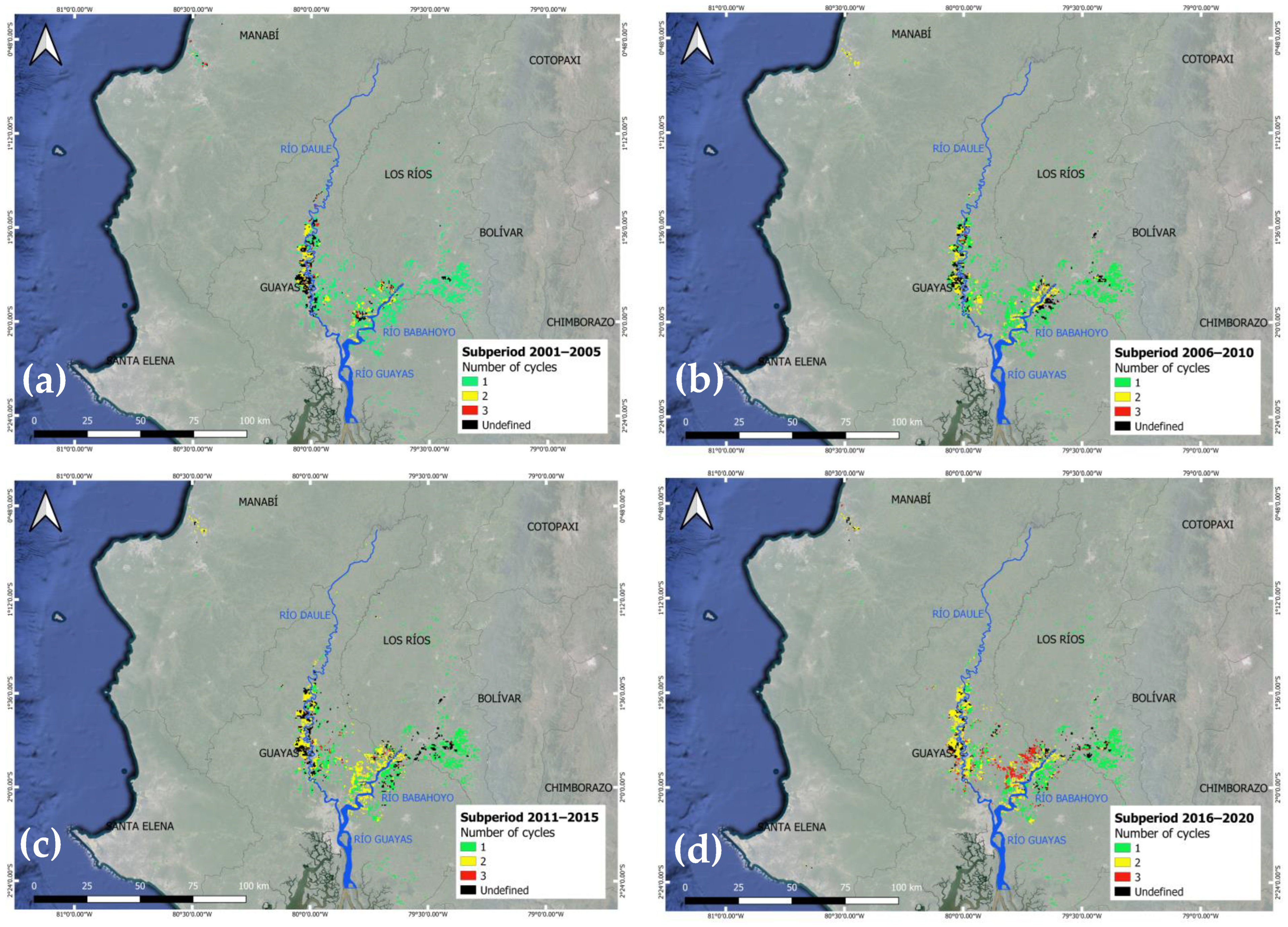
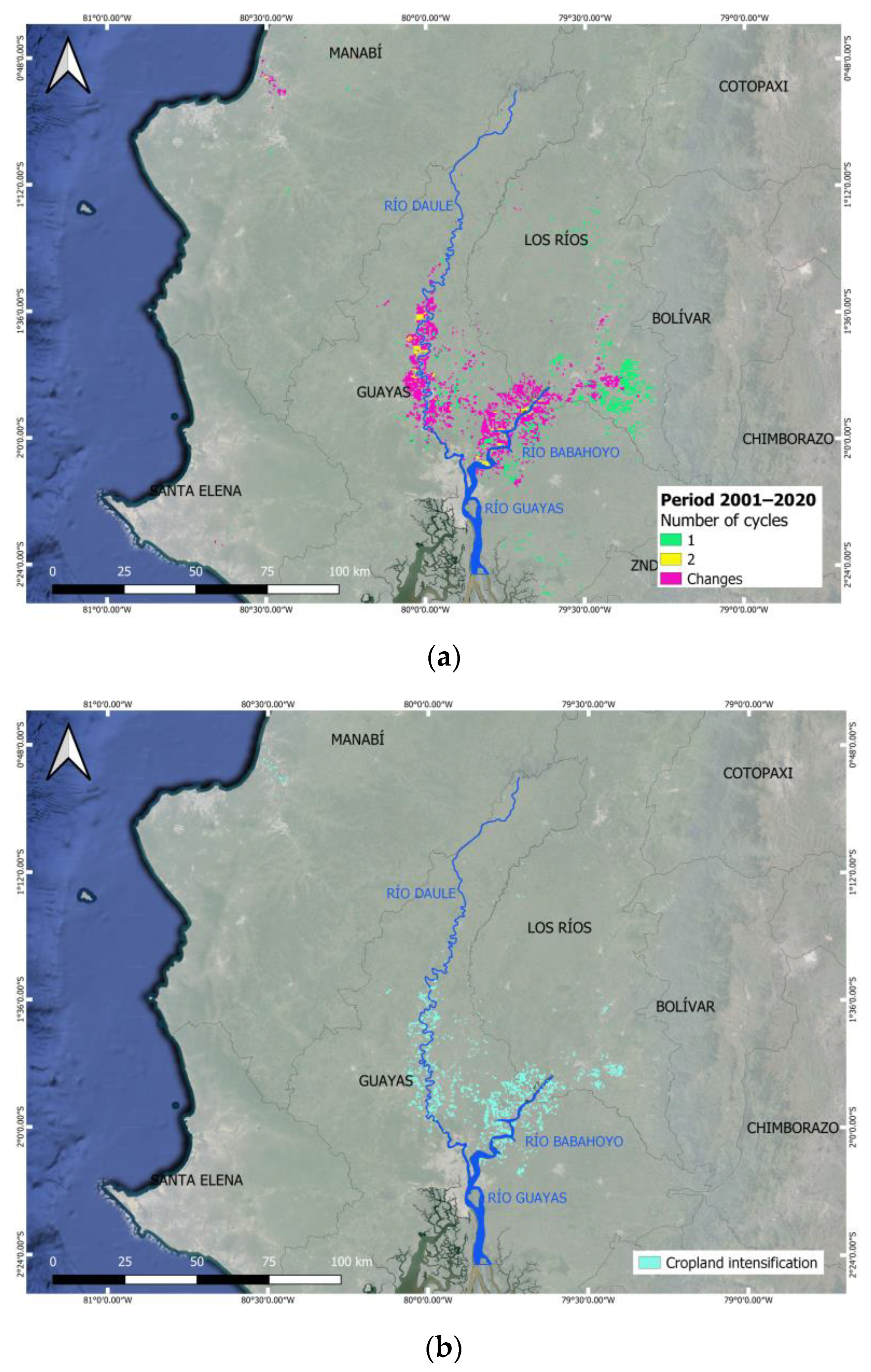
2.6. Assessment of Crop Intensification

The cropping intensity was compared between the subperiods in order to identify areas with a constant or variable number of crop growth cycles, that is, with one, two, and three NDVI seasonal cycles. Finally, in order to find increasing or decreasing trends at pixel level within the areas with different cropping intensities, linear regression models were used. The frequencies at the maximum ordinates were used as input assuming that lower frequencies mean a lower number of cycles. Thus, positive slopes mean that the number of intra-annual cycles increases across subperiods and vice versa. Several pixel examples with low noise content (high FK values) were selected to illustrate the main different crop dynamics found across the study area, some of them with a constant unimodal or bimodal cropping intensity and others with an increasing trend in the number of crop growth cycles.

2.7. Validation of the Cropping System Classification with MAG Information

The cropping systems found with the periodogram approach could be validated only with the MAG information in the last subperiod (2016–2020) due to the lack of field data during the entire study period. For this purpose, pixels with at least 80% of their surface with a dominant single-, double-, or triple-cropping system during the 5-year subperiod were selected, that is, cultivated one, two, or three times every year in at least four out of the five years. Rice and maize were treated separately to facilitate the interpretation. Therefore, a total number of 756 pixels were selected, among them, 662 and 72 correspond to a dominant single-cropping of rice and maize, respectively, and 22 to a dominant double-cropping of rice. According to the MAG information, there were no pixels with a dominant triple-cropping or undefined pattern in either of the two crop types.

3. Results

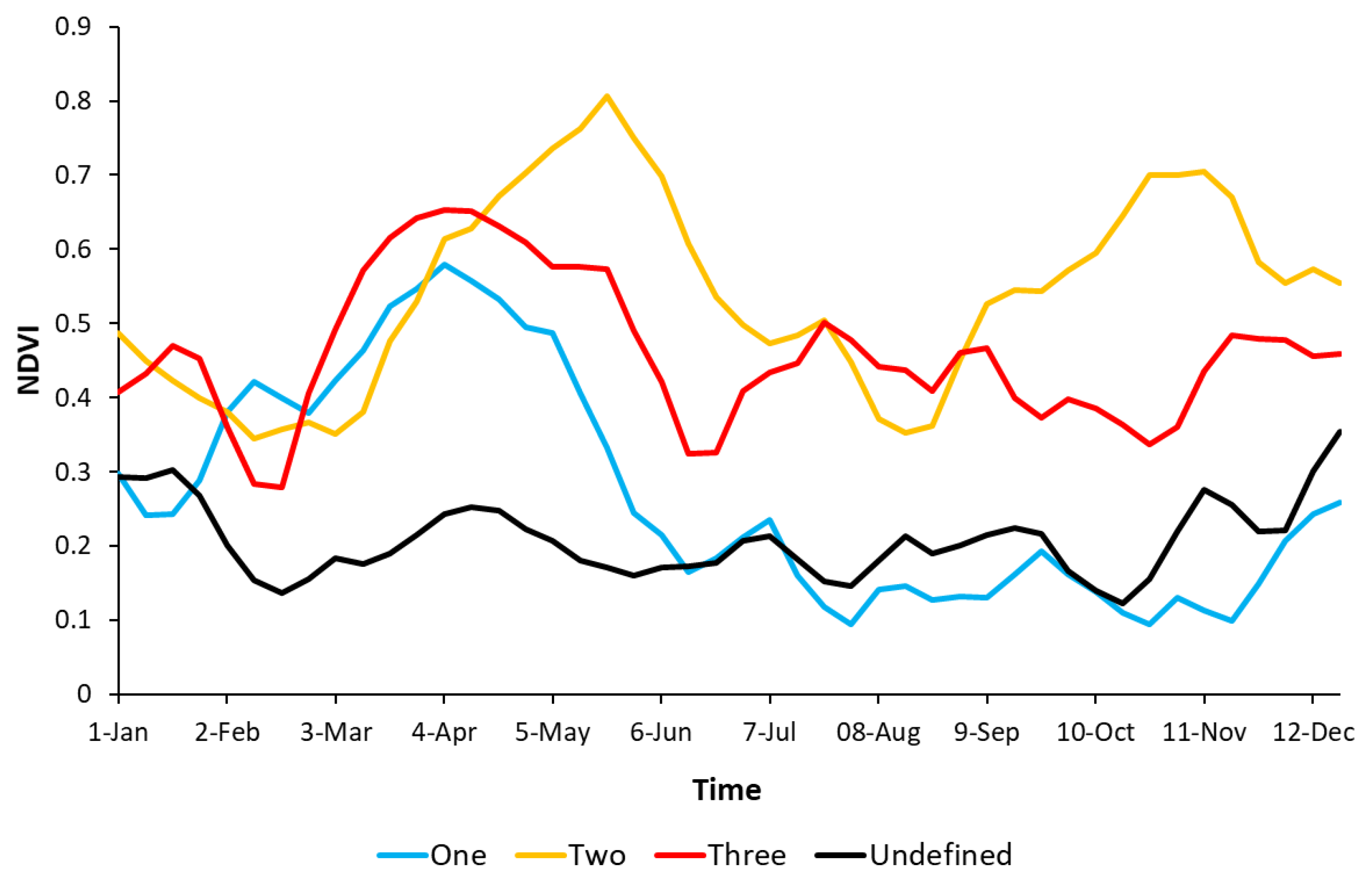
3.1. NDVI Mean Seasonal Cycle

Figure 2 shows several examples of the NDVI mean seasonal cycle for the subperiod 2016–2020 representative of each cropping system. Single-cropping in cyan shows one intra-annual cycle reaching the maximum value in April. Double-cropping in yellow shows two cycles per year with maxima in May and November in which NDVI values are higher than 0.7. Triple-cropping in red shows three seasonal cycles per year reaching the maxima in April, July, and November. NDVI average year does not show any relevant seasonal cycle when there is not a clear cropping system (black).

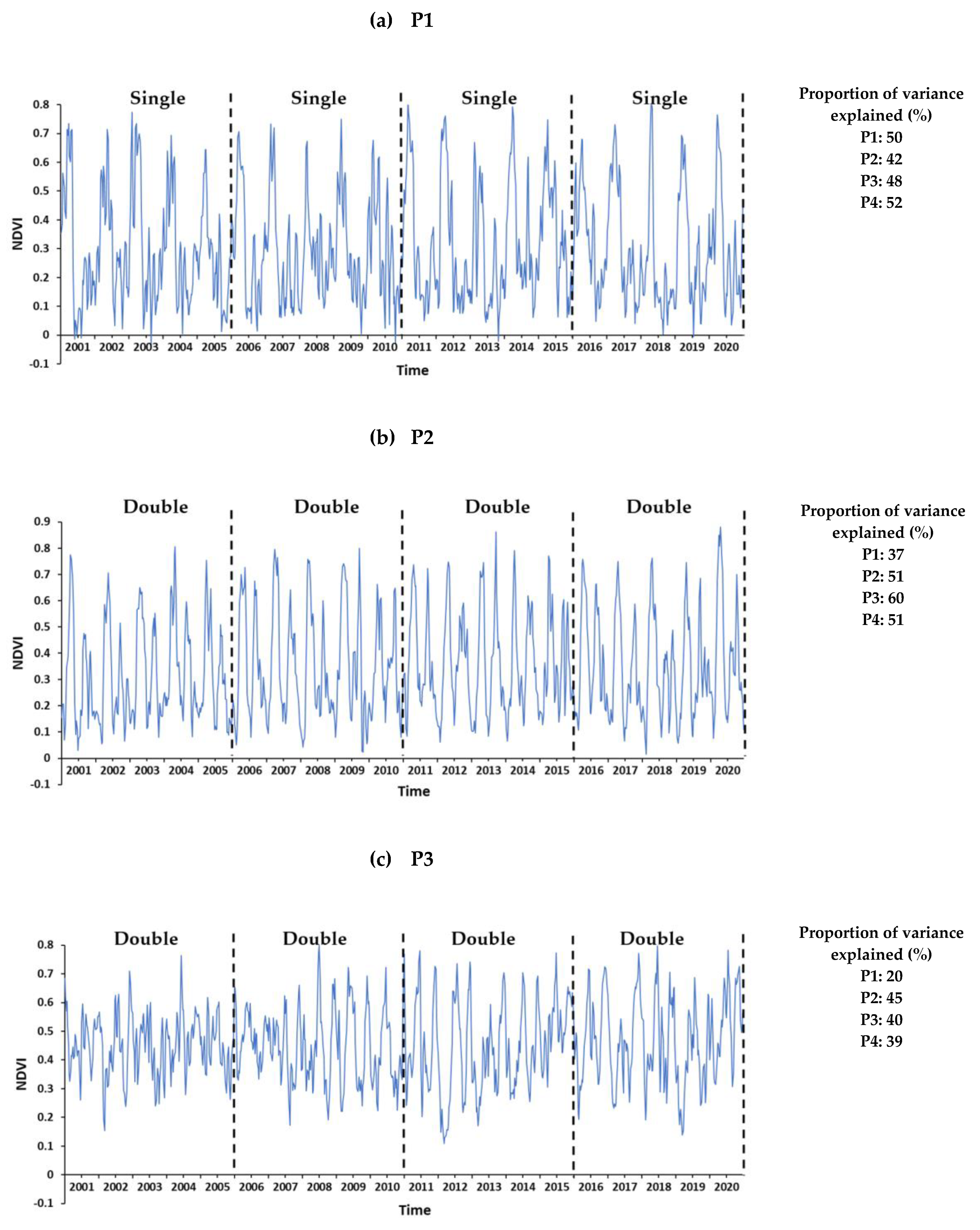
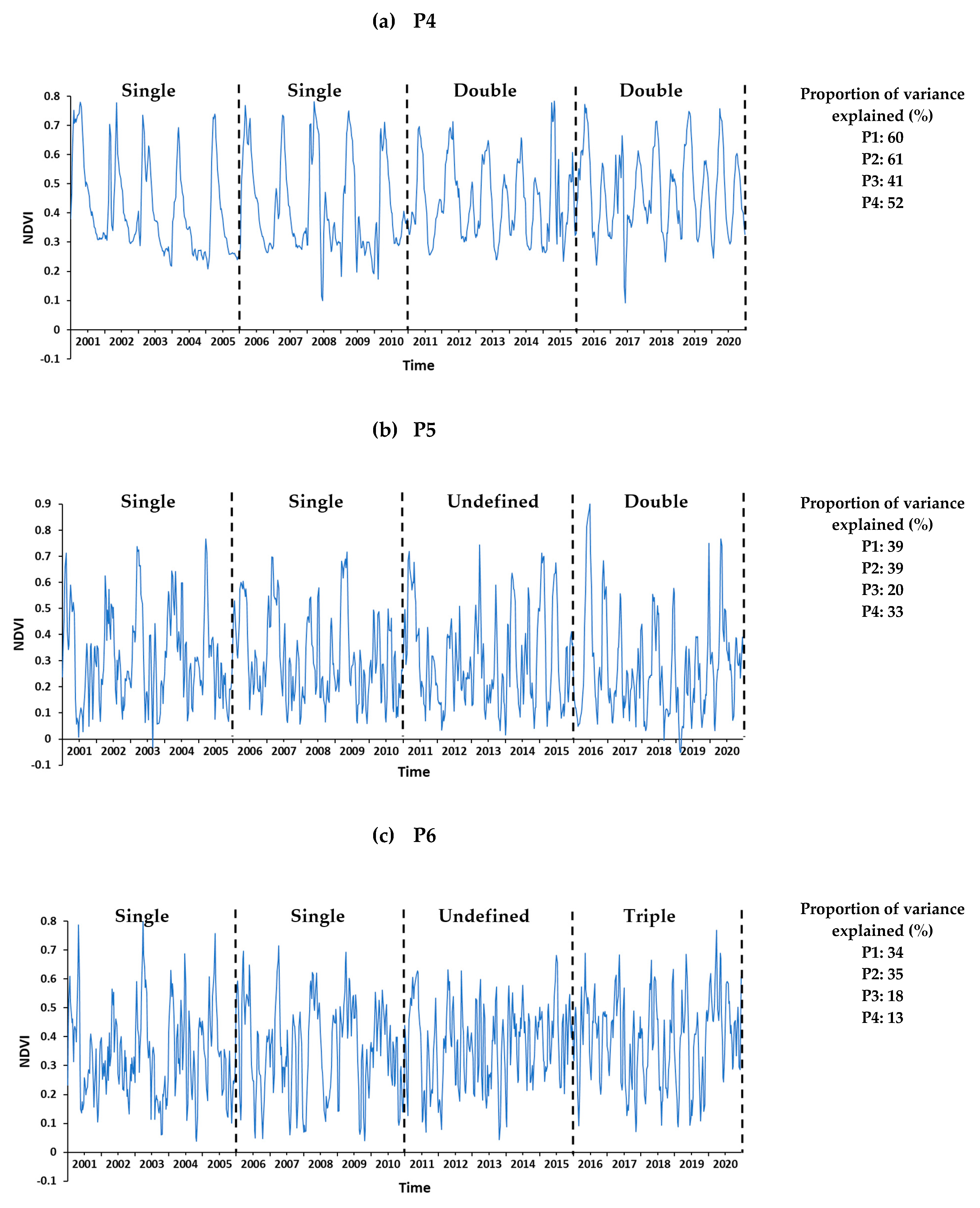
3.2. Time Series Seasonality Patterns and Cropping Systems

Figure 3 shows several examples of NDVI time series (a) and periodograms (b) for the subperiod 2016–2020 and for the different cropping systems. Croplands with a dominant single-, double-, and triple-cropping system within this subperiod show the maximum ordinate of the NDVI periodogram at periods 46, 23, and 15.3 respectively. Croplands with a maximum ordinate at a different period presented an unclear seasonal pattern during the whole subperiod.

Less than one percent of the cropland pixels show white noise series according to the Fisher kappa (FK) test in at least one subperiod, and were removed from the analysis. Particularly,

Table 3. Significance of NDVI time series periodicity for selected pixels prototypical with different number of intra-annual cycles per year (c/y).

Cropping Pattern		Period		Maximum Ordinate	Sum of All Ordinates	Ratio M.O./ΣP	FK Test
	46	23	15.3
	1 c/y	2 c/y	3 c/y	M.O.	ΣP	(%)
Single	4.1450	0.5200	0.1250	1st col.	8.1268	51.00	58.14
Double	0.1559	3.3660	0.0451	2nd col.	7.0348	47.85	54.55
Triple	0.5558	0.3758	1.5387	3rd col.	5.0635	30.39	34.65
Undefined	0.1201	0.0573	0.1905	0.2528	3.2001	7.90	9.92

M.O.: Maximum ordinate, ΣP: Sum of all periodogram ordinates. Periods 46, 23, and 15.3 corresponds to 1, 2, and 3 cycles per year, respectively.

shows a summary of spectral analysis statistics for the 5-year NDVI time series examples of cropland pixels with different seasonal patterns shown in Figure 3. Single-, double-, and triple-cropping patterns show high values of FK and a high proportion of variance explained of NDVI series in the periods 46, 23, and 15.3, respectively, indicating that their periodic components are highly significant within the subperiod 2016–2020. Conversely, the cropland pixel with an undefined pattern shows a lower FK value and near to the critical value due to the low variance of the time series by the highest ordinate value at a period different from 46, 23, and 15.3.

Figure 4 shows the spatial distribution of the cropping systems for the different subperiods 2001–2005 (a), 2006–2010 (b), 2011–2015 (c), and 2016–2020 (d). Areas with one, two, and three crop growth cycles are displayed in green, yellow, and red, respectively. Areas with an undefined seasonality are colored in black. Double- and triple-cropping systems are mainly located in the surroundings areas of Daule and Babahoyo rivers, whereas croplands with one seasonal cycle can be found in areas further away from these watercourses.

Table 4. Surfaces with single-, double-, triple-, and undefined cropping systems across the different subperiods as well as the equivalent sown surfaces considering single-, double-, and triple-cropping systems. Values are in hectares (ha).

Subperiods	Cropping System
	Single	Double	Triple	Undefined	Equivalent Sown Surface
2001–2005	67,350	9625	1925	10,325	92,375
2006–2010	62,975	15,025	600	10,625	94,825
2011–2015	47,450	25,475	1,725	14,575	103,575
2016–2020	46,025	24,400	10,450	8350	126,175

summarizes the surface occupied by each cropping system across the four subperiods. The surface with single-cropping decreased from more than 60,000 ha in the first subperiod to less than 50,000 ha in the last two subperiods. In contrast, areas with double-cropping increased by around 10,000 ha since the third subperiod, and areas with triple-cropping multiplied by more than six from the third to the fourth subperiod, reaching more than 10,000 ha. Finally, areas with an undefined cropping pattern decreased by approximately 40% from the third to the last subperiod, reaching an extent lower than 8500 ha. Therefore, the equivalent sown surface considering single-, double-, and triple-cropping systems increased by 36.6% from the first to the last subperiod, which is an increment of 33,800 ha.

Figure 5a shows the spatial distribution of rice and maize areas with a constant and variable cropping system throughout the period 2001–2020, which constitutes around 40% and 60% of the study area, respectively. Therefore, croplands with one and two seasonal cycles across all the subperiods are colored in green and yellow, respectively. Areas with changes in the number of crop growth cycles are displayed in magenta. The single-cropping system is the most widespread, remaining constant at approximately 37.1%, mainly located in the furthest areas from the watercourses. In contrast, cropland surfaces with a constant double-cropping system in all subperiods constitute only 3.8% and are mainly situated close to the rivers. There is no surface with a constant triple-cropping system across all the subperiods. Figure 6a,b show time series of croplands with constant single- and double-cropping, respectively. In all subperiods, the variance explained by periods 46 and 23 is high and similar in all subperiods. Figure 6c shows also double-cropping for all the years, but with a clear difference from the end of the first subperiod, with the higher variance explained in the last subperiods.

Most of the surface near the rivers experienced seasonal changes in terms of the number of crop growth cycles. Approximately 70% of this area showed an increase, leading to cropland intensification (Figure 5b), while the remaining 30% exhibited a decreasing trend. Less than one percent of the surface did not show any trend. In addition, approximately 32% of the study area showed an undefined cropping system in at least one subperiod, whereas less than one percent presented this pattern in the 20-year study period.

Figure 7 depicts several examples of NDVI time series of cropland pixels that experienced changes in the cropping system. The variance of the series is explained by the highest ordinate within each 5-year periodogram and shown on the right. Particularly, Figure 7a,b show the most widely extended change from single- to double-cropping. In this case, the moment of the change determines the absence of a clear cropping pattern within the subperiod. For this reason, in Figure 7a, a dominant pattern could be identified in each subperiod whereas in Figure 7b, the third period was labeled as undefined. Figure 7c also shows an increase in the number of crop cycles from single- to triple-cropping systems. The location of the cropland pixels shown in Figure 6 and Figure 7 is presented in Figure 8.

Table 5. Comparison at pixel level between the cropping systems classification for the subperiod 2016–2020 with the periodogram approach and the MAG information using pure pixels of rice and maize.

		Reference
		Rice		Maize
		Single	Double	Single	Total
Classification	Single	341	4	72	417
	Double	115	11	0	126
	Triple	153	0	0	153
	Undefined	53	7	0	60
	Total	662	22	72	756

shows the comparison of the cropping system found in the subperiod 2016–2020 using the periodogram and the MAG information corresponding to pure pixels of rice and maize. The global accuracy is 56.06%. Approximately half of the rice pixels with a dominant single- or double-cropping according to MAG data were correctly classified using the periodogram approach. Most of the rice single-cropping pixels were misclassified as double- or triple-cropping whereas double-cropping pixels were mainly misclassified as undefined and single-cropping. No errors were found in maize pixels with one annual crop growth cycle.

These 756 selected pixels used for the comparison with MAG data were evaluated with more detail during the entire 20-year period. Considering only the correctly classified pixels, around 44% of the pixels labeled as rice and 96% of those labeled as maize in the last subperiod exhibited single-cropping consistently from 2001 to 2020. However, for rice pixels that displayed double-cropping in the last subperiod, only 27% maintained this pattern throughout the four subperiods. Misclassified pixels exhibited different temporal behavior. Out of the rice single-cropping instances that were mistakenly classified as double-cropping, around 38% exhibited a dominant double-cropping system for at least three subperiods. The remaining 62% of the area predominantly followed the single-cropping system. All rice double-cropping pixels wrongly classified as single-cropping presented only one crop cycle in at least three-quarters of the study period. Pixels misclassified as triple-cropping showed a high variable temporal behavior. None of the pixels showed a constant triple-cropping during the 20-year period, most of them presented this pattern in the last subperiod, whereas single-cropping is the main pattern in the previous ones. Only 10% of the pixels misclassified as an undefined cropping system class show this pattern in at least three-quarters of the whole study period.

4. Discussion

The spectral analysis of MODIS NDVI time series allowed the assessment of crop intensity by identifying changes in the number of crop growth cycles per year in rice and maize areas of Ecuador in spite of the high amount of noise of the NDVI time series. These changes, mainly driven by climatic, economic, and technical factors, showed a significant spatial coherence.

During the period 2001–2020, approximately 60% of the study area showed changes in the cropping patterns, mostly due to an increase in cropping intensity. Single-cropping was the system most widely used mainly in areas far from the rivers where there is no water available for irrigation and crops depend exclusively on precipitation to satisfy their growth requirements. However, multiple cropping practices have become more common during the last decade with the consequent intensification, especially near the Daule and Babahoyo rivers where irrigation during the dry season is possible (Figure 4, Table 4). In addition to water availability from rivers, another possible reason may be the improvements in technology during the last decades that are fostering intensification across other tropical countries around the world such as Brazil or Indonesia [17,70]. This intensification process can be seen at pixel level in Figure 7, which shows the NDVI time series of a cropland pixel with single-cropping practices in the first decade and multiple cropping practices in the second one. The multiple cropping system most widely used was double-cropping while triple-cropping was still rare [61], although in the last subperiod (2016–2020), a remarkable increase in this cropping system was observed (Table 4).

Crop intensification results were consistent with the 16% increment of production values of maize and rice fields in Ecuador through the study period reported by the National Institute of Statistics and Censuses of Ecuador (INEC) (

Table 6. Average of sown surface (ha) and production (t) as well as the yield (t/ha) of maize and rice in Ecuador per subperiod. Data from the National Institute of Statistics and Censuses of Ecuador (INEC) [55]. Only Guayas, Los Ríos, and Manabí provinces were considered.

Period	Sown Surface (ha)	Production (t)	Yield (t/ha)
2001–2005	591,228	2,009,168	3.4
2006–2010	569,214	2,048,705	3.6
2011–2015	624,820	2,434,365	3.9
2016–2020	601,244	2,340,035	3.9

) [55]. However, our results show much higher increments in sown surface (36.6%) compared to the 1.7% increase reported by INEC. The increase in yield values documented by INEC (14.7%) may be due to the underestimation of the real sown surface.

According to the FK test, most of the filtered time series contained enough information content to assess NDVI seasonality, hence, only less than one percent were white noise and were removed from the analysis. However, the validation of the cropping system maps with the MAG estimations of sown surfaces resulted in a moderate global accuracy of approximately 56%. This number may have a high level of uncertainty driven by several factors that are described below.

There was a limitation in the availability and reliability of information to validate the results. The validation was accomplished using only information from the last subperiod (2016–2020) because of the lack of MAG information prior to 2014, reducing the number of rice and maize pure pixels available for validation. In addition, the MAG validation data were obtained by visual interpretation of high-resolution satellite imagery with limited use of field information so that a certain level of uncertainty must be expected.

Cropland pixels with an undefined number of crop cycles per year represent approximately an average of 12% of the study area per subperiod. The existence of different cropping systems within each 5-year period due to the change in cropping management practices may result in an undefined pattern or a decrease in the proportion of the variance explained of the time series by the dominant period (i.e., 46, 23, or 15.3). For instance, Figure 7b shows an NDVI time series of a cropland pixel with an undefined cropping system in the third period, when there is a change from single- to double-cropping, which results in a mixture of patterns with a 20% of variance explained by the dominant period against values higher than 30% in the other subperiods. In addition, the high noise content in the NDVI time series because of persistent cloudiness in the region may result in the appearance of an undefined pattern but seems not to be the most important reason, because only one percent of pixels within this class show this pattern during all the subperiods.

Although it would be expected that the implantation of irrigation systems would lead to a permanent change from one crop cycle to two, there are other factors that may have an influence on the number of crop growth cycles and, therefore, on the significance of the dominant periodicity. Figure 9 shows the annual evolution of the sown and harvested surfaces (ha) as well as yield (t/ha) for rice and maize in Ecuador. While yield values show a sustained increasing trend indicating a steady intensification process, the sown and harvested surfaces show a significant inter-annual variability that may be caused by the variations in the number of crop growth cycles. In this regard, climatic or economic factors determine farmers’ decisions and crop development. For instance, the severe drought in 2011 [71,72] resulted in a strong decrease in the sown and harvested surfaces but only a slight reduction in yield values. A remarkable event was also the decrease in grain prices in 2017 in Ecuador [73], which may have forced farmers not to cultivate their fields due to the lack of rentability with the consequently average yield reduction in that year.

Another fact that may increase uncertainty is the variable sowing and harvest dates, and, consequently, the duration of the crop growth is not exact every year, affecting the NDVI periodicity and making the detection of the number of crop cycles difficult. In this regard, rice areas with 2.5 and 2.6 crop growth cycles in a year were found and classified as undefined. The presence of weeds can also impact the NDVI signal; however, their influence is restricted by the application of herbicides before cultivation and their limited growth during the dry periods. Finally, the existence of small fields with high heterogeneity in cropping systems makes it complicated to define patterns at pixel level since they have almost 25 ha and surpass by far the common size of a single field in the study area, which ranges between 1 and 10 ha [74]. This is a common problem when working with moderate spatial resolution images as MODIS data [75,76].

In tropical areas, the development of new techniques for assessing vegetation dynamics under cloudy conditions is necessary [77,78]. In this sense, the periodogram approach used in this study has shown to be useful in tropical areas because it considers the whole observations of the time series to extract relevant phenological information, being more noise-independent and not dealing with specific phenological dates. Therefore, the periodogram approach has two main advantages. Firstly, its simplicity and high operability; the identification of the maximum ordinate of the NDVI periodogram enables the mapping of croplands with single, double, and triple intensities without the need of setting vegetation index threshold values as in other studies [32,34,36]. Secondly, it is not highly dependent on the filtering method selected for smoothing time series as the phenometric approach [39]. In addition, splitting the 20-year time series into subperiods provided relevant information to evaluate crop intensification when calculating their respective periodograms. If the periodogram was calculated using the entire time series, lower FK values and a reduced proportion of the variance explained of the series in the dominant period would be expected in areas subjected to crop intensification due to the mixture of cropping patterns. Therefore, considering subperiods was more informative than working with the complete time series.

Nowadays, assessing agricultural areas in the tropics with optical remote sensing data is still challenging. In this sense, the periodogram approach using NDVI time series has demonstrated a high capability to map agricultural intensification in Ecuador dealing with a noisy time series. In spite of the moderate validation results, this information is crucial for decision-makers to develop agricultural policies that ensure food security while maintaining sustainable practices [7]. Monitoring areas with multiple cropping practices could help to reduce the negative effects of intensification [9,10,11,12], especially in the tropics, where during the last decades these practices have experienced an increasing trend [17,70].

In the near future, it will be possible to reduce the uncertainty of agricultural intensification with the availability of longer time series at higher spatial resolution such as those provided by Sentinel-2 satellites [12,36]. More detailed and updated information will be accessible for public authorities and citizens helping them to make decisions and be aware of global change and food security.

5. Conclusions

In this research, the spectral analysis of a 20-year MODIS NDVI time series has demonstrated a high capability to map cropland intensification in Ecuador during the period 2001–2020 by comparing the number of crop growth cycles per year between four subperiods. The criteria based on the maximum ordinate of NDVI periodogram at the periods 46, 23, and 15.3 enabled the identification of croplands with single-, double-, and triple-cropping, respectively.

Approximately 60% of the rice and maize areas suffered changes in the cropping systems and 70% of this surface showed an increase in cropping intensity, being mainly distributed near water bodies where irrigation is possible during the dry season. Single-cropping is the most widely used practice especially during the first decade, experiencing a decrease of more than ten thousand hectares across the study period. In contrast, area under multi-cropping systems increased during the second decade, with growing two crops per year being more extended than triple cropping.

The use of the long MODIS time series with highly frequent observations enabled the mapping of cropping intensities with high spatial coherence in spite of the moderate spatial resolution of imagery and noisy time series. Therefore, this simple and high operative methodology could be easily applied worldwide across different environmental conditions, probably obtaining more accurate results when working with series with a lower noise content. This work opens the door to further studies using other vegetation indices time series as well as higher resolution imagery, being highly useful in developing countries and tropical areas with high cloudiness.

References

1. Liu, L.; Xu, X.; Zhuang, D.; Chen, X.; Li, S. Changes in the Potential Multiple Cropping System in Response to Climate Change in China from 1960–2010. PLoS ONE 2013, 8, e80990. [Google Scholar] [CrossRef]
2. FAO. FAOSTAT. Available online: https://www.fao.org/faostat/en/#home (accessed on 2 December 2022).
3. Battude, M.; Al Bitar, A.; Morin, D.; Cros, J.; Huc, M.; Marais Sicre, C.; Le Dantec, V.; Demarez, V. Estimating Maize Biomass and Yield over Large Areas Using High Spatial and Temporal Resolution Sentinel-2 like Remote Sensing Data. Remote Sens. Environ. 2016, 184, 668–681. [Google Scholar] [CrossRef]
4. FAO’s Director-General on How to Feed the World in 2050. Popul. Dev. Rev. 2009, 35, 837–839. [CrossRef]
5. Godfray, H.C.J.; Beddington, J.R.; Crute, I.R.; Haddad, L.; Lawrence, D.; Muir, J.F.; Pretty, J.; Robinson, S.; Thomas, S.M.; Toulmin, C. Food Security: The Challenge of Feeding 9 Billion People. Science 2010, 327, 812–818. [Google Scholar] [CrossRef]
6. Tilman, D.; Balzer, C.; Hill, J.; Befort, B.L. Global Food Demand and the Sustainable Intensification of Agriculture. Proc. Natl. Acad. Sci. USA 2011, 108, 20260–20264. [Google Scholar] [CrossRef] [PubMed]
7. Guo, Y.; Xia, H.; Pan, L.; Zhao, X.; Li, R. Mapping the Northern Limit of Double Cropping Using a Phenology-Based Algorithm and Google Earth Engine. Remote Sens. 2022, 14, 1004. [Google Scholar] [CrossRef]
8. Yan, H.; Liu, F.; Qin, Y.; Niu, Z.; Doughty, R.; Xiao, X. Tracking the Spatio-Temporal Change of Cropping Intensity in China during 2000–2015. Environ. Res. Lett. 2019, 14, 035008. [Google Scholar] [CrossRef]
9. Clark, M.; Tilman, D. Comparative Analysis of Environmental Impacts of Agricultural Production Systems, Agricultural Input Efficiency, and Food Choice Comparative Analysis of Environmental Impacts of Agricultural Production Systems, Agricultural Input Efficiency, and Food. Environ. Res. Lett. 2017, 12, 064016. [Google Scholar] [CrossRef]
10. Weller, S.; Janz, B.; Jörg, L.; Kraus, D.; Racela, H.S.U.; Wassmann, R.; Butterbach-Bahl, K.; Kiese, R. Greenhouse Gas Emissions and Global Warming Potential of Traditional and Diversified Tropical Rice Rotation Systems. Glob. Chang. Biol. 2016, 22, 432–448. [Google Scholar] [CrossRef]
11. Zabel, F.; Delzeit, R.; Schneider, J.M.; Seppelt, R.; Mauser, W.; Václavík, T. Global Impacts of Future Cropland Expansion and Intensification on Agricultural Markets and Biodiversity. Nat. Commun. 2019, 10, 2844. [Google Scholar] [CrossRef] [PubMed]
12. He, Y.; Dong, J.; Liao, X.; Sun, L.; Wang, Z.; You, N.; Li, Z.; Fu, P. Examining Rice Distribution and Cropping Intensity in a Mixed Single- and Double-Cropping Region in South China Using All Available Sentinel 1/2 Images. Int. J. Appl. Earth Obs. Geoinf. 2021, 101, 102351. [Google Scholar] [CrossRef]
13. Biradar, C.M.; Xiao, X. Quantifying the Area and Spatial Distribution of Double- and Triple-Cropping Croplands in India with Multi-Temporal MODIS Imagery in 2005. Int. J. Remote Sens. 2011, 32, 367–386. [Google Scholar] [CrossRef]
14. Gray, J.; Friedl, M.; Frolking, S.; Ramankutty, N.; Nelson, A.; Gumma, M.K. Mapping Asian Cropping Intensity with MODIS. IEEE J. Sel. Top. Appl. Earth Obs. Remote Sens. 2014, 7, 3373–3379. [Google Scholar] [CrossRef]
15. Han, J.; Zhang, Z.; Luo, Y.; Cao, J.; Zhang, L.; Zhuang, H.; Cheng, F.; Zhang, J.; Tao, F. Annual Paddy Rice Planting Area and Cropping Intensity Datasets and Their Dynamics in the Asian Monsoon Region from 2000 to 2020. Agric. Syst. 2022, 200, 103437. [Google Scholar] [CrossRef]
16. Peng, D.; Huete, A.R.; Huang, J.; Wang, F.; Sun, H. Detection and Estimation of Mixed Paddy Rice Cropping Patterns with MODIS Data. Int. J. Appl. Earth Obs. Geoinf. 2011, 13, 13–23. [Google Scholar] [CrossRef]
17. Hu, Q.; Xiang, M.; Chen, D.; Zhou, J.; Wu, W.; Song, Q. Global Cropland Intensification Surpassed Expansion between 2000 and 2010: A Spatio-Temporal Analysis Based on GlobeLand30. Sci. Total Environ. 2020, 746, 141035. [Google Scholar] [CrossRef]
18. Ministerio del Ambiente, Agua y Transición Ecológica (MAATE). Plan Nacional de Riego y Drenaje 2021–2026. Resumen Ejecutivo; MAATE: Quito, Ecuador, 2022. [Google Scholar]
19. Mosleh, M.K.; Hassan, Q.K. Development of a Remote Sensing-Based “Boro” Rice Mapping System. Remote Sens. 2014, 6, 1938. [Google Scholar] [CrossRef]
20. GEOGLAM Group on Earth Observations Global Agricultural Monitoring Initiative. Available online: https://earthobservations.org/geoglam.php# (accessed on 19 December 2022).
21. Boschetti, M.; Busetto, L.; Manfron, G.; Laborte, A.; Asilo, S.; Pazhanivelan, S.; Nelson, A. PhenoRice: A Method for Automatic Extraction of Spatio-Temporal Information on Rice Crops Using Satellite Data Time Series. Remote Sens. Environ. 2017, 194, 347–365. [Google Scholar] [CrossRef]
22. Gumma, M.K.; Nelson, A.; Thenkebail, P.S.; Singh, A.N. Mapping Rice Areas of South Asia Using MODIS Multitemporal Data. J. Appl. Remote Sens. 2011, 5, 053547. [Google Scholar] [CrossRef]
23. Mishra, B.; Busetto, L.; Boschetti, M.; Laborte, A.; Nelson, A. RICA: A Rice Crop Calendar for Asia Based on MODIS Multi Year Data. Int. J. Appl. Earth Obs. Geoinf. 2021, 103, 102471. [Google Scholar] [CrossRef]
24. Wang, Y.; Zang, S.; Tian, Y. Mapping Paddy Rice with the Random Forest Algorithm Using MODIS and SMAP Time Series. Chaos Solitons Fractals 2020, 140, 110116. [Google Scholar] [CrossRef]
25. Johnson, D.M.; Rosales, A.; Mueller, R.; Reynolds, C.; Frantz, R.; Anyamba, A.; Pak, E.; Tucker, C. USA Crop Yield Estimation with MODIS NDVI: Are Remotely Sensed Models Better than Simple Trend Analyses? Remote Sens. 2021, 13, 4227. [Google Scholar] [CrossRef]
26. Jabal, Z.K.; Khayyun, T.S.; Alwan, I.A. Impact of Climate Change on Crops Productivity Using MODIS-NDVI Time Series. Civ. Eng. J. 2022, 8, 1136–1156. [Google Scholar] [CrossRef]
27. Guan, X.; Huang, C.; Liu, G.; Meng, X.; Liu, Q. Mapping Rice Cropping Systems in Vietnam Using an NDVI-Based Time-Series Similarity Measurement Based on DTW Distance. Remote Sens. 2016, 8, 19. [Google Scholar] [CrossRef]
28. Liu, L.; Huang, J.; Xiong, Q.; Zhang, H.; Song, P.; Huang, Y.; Dou, Y.; Wang, X. Optimal MODIS Data Processing for Accurate Multi-Year Paddy Rice Area Mapping in China. GIsci Remote Sens. 2020, 57, 687–703. [Google Scholar] [CrossRef]
29. Luintel, N.; Ma, W.; Ma, Y.; Wang, B.; Xu, J.; Dawadi, B.; Mishra, B. Tracking the Dynamics of Paddy Rice Cultivation Practice through MODIS Time Series and PhenoRice Algorithm. Agric. For. Meteorol. 2021, 307, 108538. [Google Scholar] [CrossRef]
30. Lunetta, R.S.; Shao, Y.; Ediriwickrema, J.; Lyon, J.G. Monitoring Agricultural Cropping Patterns across the Laurentian Great Lakes Basin Using MODIS-NDVI Data. Int. J. Appl. Earth Obs. Geoinf. 2010, 12, 81–88. [Google Scholar] [CrossRef]
31. Zhang, G.; Xiao, X.; Dong, J.; Kou, W.; Jin, C.; Qin, Y.; Zhou, Y.; Wang, J.; Menarguez, M.A.; Biradar, C. Mapping Paddy Rice Planting Areas through Time Series Analysis of MODIS Land Surface Temperature and Vegetation Index Data. ISPRS J. Photogramm. Remote Sens. 2015, 106, 157–171. [Google Scholar] [CrossRef] [PubMed]
32. Sakamoto, T.; van Nguyen, N.; Ohno, H.; Ishitsuka, N.; Yokozawa, M. Spatio-Temporal Distribution of Rice Phenology and Cropping Systems in the Mekong Delta with Special Reference to the Seasonal Water Flow of the Mekong and Bassac Rivers. Remote Sens. Environ. 2006, 100, 1–16. [Google Scholar] [CrossRef]
33. Estel, S.; Kuemmerle, T.; Levers, C.; Baumann, M.; Hostert, P. Mapping Cropland-Use Intensity across Europe Using MODIS NDVI Time Series. Environ. Res. Lett. 2016, 11, 024015. [Google Scholar] [CrossRef]
34. Ding, M.; Chen, Q.; Xiao, X.; Xin, L.; Zhang, G.; Li, L. Variation in Cropping Intensity in Northern China from 1982 to 2012 Based on GIMMS-NDVI Data. Sustainability 2016, 8, 1123. [Google Scholar] [CrossRef]
35. Kontgis, C.; Schneider, A.; Ozdogan, M. Mapping Rice Paddy Extent and Intensification in the Vietnamese Mekong River Delta with Dense Time Stacks of Landsat Data. Remote Sens. Environ. 2015, 169, 255–269. [Google Scholar] [CrossRef]
36. Liu, L.; Xiao, X.; Qin, Y.; Wang, J.; Xu, X.; Hu, Y.; Qiao, Z. Mapping Cropping Intensity in China Using Time Series Landsat and Sentinel-2 Images and Google Earth Engine. Remote Sens. Environ. 2020, 239, 111624. [Google Scholar] [CrossRef]
37. Gao, F.; Zhang, X. Mapping Crop Phenology in Near Real-Time Using Satellite Remote Sensing: Challenges and Opportunities. J. Remote Sens. 2021, 2021, 8379391. [Google Scholar] [CrossRef]
38. Ganguly, S.; Friedl, M.A.; Tan, B.; Zhang, X.; Verma, M. Land Surface Phenology from MODIS: Characterization of the Collection 5 Global Land Cover Dynamics Product. Remote Sens. Environ. 2010, 114, 1805–1816. [Google Scholar] [CrossRef]
39. Chen, C.-F. Mapping Double-Cropped Irrigated Rice Fields in Taiwan Using Time-Series Satellite Pour I’Observation de La Terre Data. J. Appl. Remote Sens. 2011, 5, 053528. [Google Scholar] [CrossRef]
40. Hamilton, J.D. Time Series Analysis; Princeton University Press: Princeton, NJ, USA, 1994; ISBN 0-691-04289-6. [Google Scholar]
41. Bloomfield, P. Fourier Analysis of Time Series: An Introduction, 2nd ed.; John Wiley & Sons: New York, NY, USA, 2000; ISBN 0-471-88948-2. [Google Scholar]
42. Bush, E.R.; Abernethy, K.A.; Jeffery, K.; Tutin, C.; White, L.; Dimoto, E.; Dikangadissi, J.T.; Jump, A.S.; Bunnefeld, N. Fourier Analysis to Detect Phenological Cycles Using Long-Term Tropical Field Data and Simulations. Methods Ecol. Evol. 2017, 8, 530–540. [Google Scholar] [CrossRef]
43. Menenti, M.; Azzali, S.; Verhoef, W.; van Swol, R. Mapping Agroecological Zones and Time Lag in Vegetation Growth by Means of Fourier Analysis of Time Series of NDVI Images. Adv. Space Res. 1993, 13, 233–237. [Google Scholar] [CrossRef]
44. Olsson, L.; Eklundh, L. Fourier Series for Analysis of Temporal Sequences of Satellite Sensor Imagery. Int. J. Remote Sens. 1994, 15, 3735–3741. [Google Scholar] [CrossRef]
45. Andres, L.; Salas, W.A.; Skole, D. Fourier Analysis of Multi-Temporal AVHRR Data Applied to a Land Cover Classification. Int. J. Remote Sens. 1994, 15, 1115–1121. [Google Scholar] [CrossRef]
46. Azzali, S.; Menenti, M. Mapping Vegetation-Soil-Climate Complexes in Southern Africa Using Temporal Fourier Analysis of NOAA-AVHRR NDVI Data. Int. J. Remote Sens. 2000, 21, 973–996. [Google Scholar] [CrossRef]
47. Jakubauskas, M.E.; Legates, D.R. Harmonic Analysis of Time-Series AVHRR NDVI Data for Characterizing US Great Plains Land Use/Land Cover. Int. Arch. Photogramm. Remote Sens. 2000, 33, 384–389. [Google Scholar]
48. Jakubauskas, M.E.; Legates, D.R.; Kastens, J.H. Harmonic Analysis of Time-Series AVHRR NDVI Data. Photogramm. Eng. Remote Sens. 2001, 67, 461–470. [Google Scholar]
49. Jakubauskas, M.E.; Legates, D.R.; Kastens, J.H. Crop Identification Using Harmonic Analysis of Time-Series AVHRR NDVI Data. Comput. Electron. Agric. 2002, 37, 127–139. [Google Scholar] [CrossRef]
50. Mingwei, Z.; Qingbo, Z.; Zhongxin, C.; Jia, L.; Yong, Z.; Chongfa, C. Crop Discrimination in Northern China with Double Cropping Systems Using Fourier Analysis of Time-Series MODIS Data. Int. J. Appl. Earth Obs. Geoinf. 2008, 10, 476–485. [Google Scholar] [CrossRef]
51. Canisius, F.; Turral, H.; Molden, D. Fourier Analysis of Historical NOAA Time Series Data to Estimate Bimodal Agriculture. Int. J. Remote Sens. 2007, 28, 5503–5522. [Google Scholar] [CrossRef]
52. Schuster, A. On the Investigation of Hidden Periodicities with Application to a Supposed 26 Day Period of Meteorological Phenomena. J. Geophys. Res. 1898, 3, 13–41. [Google Scholar] [CrossRef]
53. Huesca, M.; Litago, J.; Palacios-Orueta, A.; Montes, F.; Sebastián-López, A.; Escribano, P. Assessment of Forest Fire Seasonality Using MODIS Fire Potential: A Time Series Approach. Agric. Meteorol. 2009, 149, 1946–1955. [Google Scholar] [CrossRef]
54. Recuero, L.; Litago, J.; Pinzón, J.E.; Huesca, M.; Moyano, M.C.; Palacios-Orueta, A. Mapping Periodic Patterns of Global Vegetation Based on Spectral Analysis of NDVI Time Series. Remote Sens. 2019, 11, 2497. [Google Scholar] [CrossRef]
55. INEC Instituto Nacional de Estadística y Censos de Ecuador. Available online: https://www.ecuadorencifras.gob.ec/institucional/home/ (accessed on 23 January 2023).
56. Beck, H.E.; Zimmermann, N.E.; McVicar, T.R.; Vergopolan, N.; Berg, A.; Wood, E.F. Present and Future Köppen-Geiger Climate Classification Maps at 1-Km Resolution. Sci. Data 2018, 5, 180214. [Google Scholar] [CrossRef]
57. Kottek, M.; Grieser, J.; Beck, C.; Rudolf, B.; Rubel, F. World Map of the Köppen-Geiger Climate Classification Updated. Meteorol. Z. 2006, 15, 259–263. [Google Scholar] [CrossRef] [PubMed]
58. Muñoz-Salcedo, M.; Peci-López, F.; Táboas, F. An Empirical Correction Model for Remote Sensing Data of Global Horizontal Irradiance in High-Cloudiness-Index Locations. Remote Sens. 2022, 14, 5496. [Google Scholar] [CrossRef]
59. MAG Geoportal Del Agro Ecuatoriano. Ministerio de Agricultura y Ganadería, Gobierno de La República de Ecuador. Available online: http://geoportal.agricultura.gob.ec/geonetwork/srv/spa/catalog.search#/home (accessed on 10 January 2022).
60. Vermote, E. MOD09A1 MODIS/Terra Surface Reflectance 8-Day L3 Global 500m SIN Grid V006; NASA EOSDIS Land Processes Distributed Active Archive Center: Sioux Falls, SD, USA, 2015. [Google Scholar] [CrossRef]
61. Zambrano, C.E.; Andrade Arias, M.S.; Carreño Rodríguez, W.V. Factores Que Inciden En La Productividad Del Cultivo de Arroz En La Provincia de Los Ríos. Univ. Y Soc. 2019, 11, 270–277. [Google Scholar]
62. Tucker, C.J. Red and Photographic Infrared Linear Combinations for Monitoring Vegetation. Remote Sens. Environ. 1979, 8, 127–150. [Google Scholar] [CrossRef]
63. Abraham, S.; Golay, M.J.E. Smoothing and Differentiation of Data by Simplified Least Squares Procedures. Anal. Chem. 1964, 36, 1627–1639. [Google Scholar] [CrossRef]
64. Zhang, T.T.; Qi, J.G.; Gao, Y.; Ouyang, Z.T.; Zeng, S.L.; Zhao, B. Detecting Soil Salinity with MODIS Time Series VI Data. Ecol. Indic. 2015, 52, 480–489. [Google Scholar] [CrossRef]
65. Box, G.E.; Jenkins, G.M.; Reinsel, G.C. Time Series Analysis: Forecasting and Control, 3rd ed.; Prentice Hall: Englewood Cliffs, NJ, USA, 1994; ISBN 0-13-060774-6. [Google Scholar]
66. SAS Institute Inc. SAS/ETS® User’s Guide, Versión 8; SAS Institute Inc.: Cary, NC, USA, 1999. [Google Scholar]
67. Jenkins, G.M.; Watts, D.G. Spectral Analysis and Its Applications; Holden-Day Inc.: San Francisco, CA, USA, 1968. [Google Scholar]
68. Fuller, W.A. Introduction to Statistical Time Series; John Wiley and Sons: New York, NY, USA, 1976. [Google Scholar]
69. Ahdesmaki, M.; Fokianos, K.; Strimmer, K. GeneCycle: Identification of Periodically Expressed Genes 2015. Available online: https://cran.r-project.org/web/packages/GeneCycle/index.html (accessed on 26 September 2022).
70. Pires, G.F.; Abrahão, G.M.; Brumatti, L.M.; Oliveira, L.J.C.; Costa, M.H.; Liddicoat, S.; Kato, E.; Ladle, R.J. Increased Climate Risk in Brazilian Double Cropping Agriculture Systems: Implications for Land Use in Northern Brazil. Agric. Meteorol. 2016, 228–229, 286–298. [Google Scholar] [CrossRef]
71. El Universo. Ecuador Declara en Emergencia a Seis Provincias Por Sequía. Available online: https://www.eluniverso.com/2011/04/02/1/1447/ecuador-declara-emergencia-seis-provincias-sequia.html/ (accessed on 7 February 2023).
72. BBC. Ecuador Declara la Emergencia por Sequía en Seis Provincias. Available online: https://www.bbc.com/mundo/ultimas_noticias/2011/04/110402_ultnot_ecuador_sequia_emergencia_lr (accessed on 7 February 2023).
73. El Universo. Arroceros Lidian Con Bajos Precios Por Mayor Cosecha y Contrabando. Available online: https://www.eluniverso.com/noticias/2017/01/28/nota/6018754/arroceros-lidian-bajos-precios-mayor-cosecha-contrabando/ (accessed on 8 February 2023).
74. Cobos Mora, F.; Gómez Villalva, J.; Moran, E.H.; Medina Litardo, R. Sostenibilidad Del Cultivo de Arroz (Orysa sativa L.) En La Zona de Daule, Provincia Del Guayas, Ecuador. J. Sci. Res. 2020, 5, 1–16. [Google Scholar] [CrossRef]
75. Xiao, X.; Boles, S.; Liu, J.; Zhuang, D.; Frolking, S.; Li, C.; Salas, W.; Moore, B. Mapping Paddy Rice Agriculture in Southern China Using Multi-Temporal MODIS Images. Remote Sens. Environ. 2005, 95, 480–492. [Google Scholar] [CrossRef]
76. Chen, Y.; Lu, D.; Moran, E.; Batistella, M.; Dutra, L.V.; Sanches, I.D.A.; da Silva, R.F.B.; Huang, J.; Luiz, A.J.B.; de Oliveira, M.A.F. Mapping Croplands, Cropping Patterns, and Crop Types Using MODIS Time-Series Data. Int. J. Appl. Earth Obs. Geoinf. 2018, 69, 133–147. [Google Scholar] [CrossRef]
77. Eberhardt, I.D.R.; Schultz, B.; Rizzi, R.; Sanches, I.D.A.; Formaggio, A.R.; Atzberger, C.; Mello, M.P.; Immitzer, M.; Trabaquini, K.; Foschiera, W.; et al. Cloud Cover Assessment for Operational Crop Monitoring Systems in Tropical Areas. Remote Sens. 2016, 8, 219. [Google Scholar] [CrossRef]
78. Prudente, V.H.R.; Martins, V.S.; Vieira, D.C.; de Fe Silva, N.R.; Adami, M.; Sanches, I.D.A. Limitations of Cloud Cover for Optical Remote Sensing of Agricultural Areas across South America. Remote Sens. Appl. 2020, 20, 100414. [Google Scholar] [CrossRef]
Figure 2. Mean NDVI seasonal cycles for the 2016–2020 period. Croplands with one, two, and three seasonal cycles are displayed in cyan, orange, and red. Unclear seasonality in black.
Agronomy 13 02329 g002
Figure 3. Examples of NDVI time series (left) and their periodograms (right) for the period 2016–2020 of four cropland pixels prototypical of different seasonality: one seasonal cycle (a,b), two seasonal cycles (c,d), three seasonal cycles (e,f), and with an undefined pattern (g,h). Red lines separate periods of 46 MODIS observations (one year).
Agronomy 13 02329 g003
Figure 4. Spatial distribution of the different cropping patterns of pixels with more than 80% of their surface cultivated with rice and maize for the subperiods: 2001–2005 (a), 2006–2010 (b), 2011–2015 (c), and 2016–2020 (d).
Agronomy 13 02329 g004
Figure 5. (a) Spatial distribution of pixels with more than 80% of their surface cultivated with rice and maize areas with and without cropping system changes in terms of the number of crop growth cycles throughout the 2001–2020 period. (b) Agricultural areas with an increasing trend of the number of crop growth cycles (cropland intensification).
Agronomy 13 02329 g005
Figure 6. Examples of NDVI time series of cropland pixels with single-cropping (a) and double-cropping (b,c). Black lines separate 5-year subperiods. Proportions of the variance explained for the NDVI series in the periods 46 and 23 for single- and double-cropping, respectively, and for every 5-year subperiod to the right.
Agronomy 13 02329 g006
Figure 7. Examples of NDVI time series of cropland pixels with changes in the cropping system: from single- to double-cropping (a,b), from single- to triple-cropping (c). Black bars separate 5-year subperiods. Proportions of the variance for the NDVI series in the periods 46, 23, and 15.3 for single-, double-, and triple-cropping, respectively, and for every 5-year subperiod to the right.
Agronomy 13 02329 g007
Figure 8. Location of six cropland pixel examples with different cropping dynamics found across the study area throughout the period 2001–2020.
Agronomy 13 02329 g008
Figure 9. Sown and harvested surfaces (ha) and yield (t/ha) of rice and maize in Ecuador from 2002 to 2020 reported by the National Institute of Statistics and Censuses of Ecuador (INEC) [55]. Only Guayas, Los Ríos, and Manabí provinces were considered.
Agronomy 13 02329 g009