A Fertilization Decision Model for Maize, Rice, and Soybean Based on Machine Learning and Swarm Intelligent Search Algorithms

Abstract

Background: The application of base fertilizer is significant for reducing agricultural costs, non-point source pollution, and increasing crop production. However, the existing fertilization decision methods require many field observations and have high prices for popularization and application. Methods: This study proposes an innovative model integrating machine learning (ML) and swarm intelligence search algorithms to overcome the above issues. Based on historical data for maize, rice, and soybean crops, ML algorithms including random forest (RF), extreme random tree (ERT), and extreme gradient boosting (XGBoost) were evaluated for predicting crop yield. Coupled with the cuckoo search algorithm (CSA), the prime fertilization decision model (FDM) was established to discover the optimal fertilization strategy. Result: For all three crops, the yield simulation accuracy of the ERT model was the highest, with an R² and RRMSE of 0.749, 0.775, and 0.744, and 0.086, 0.051, and 0.078, respectively. Considering soil nutrient and fertilization characteristics as the determinants of yield and optimizing fertilization strategies, the proposed model can increase the average yield of maize, rice, and soybean in the study area by 23.9%, 13.3%, and 20.3%, respectively. Conclusions: The coupling model of ERT and the CSA constructed in this study can be used for the intelligent and rapid decision-making of the base fertilizer application for crops considered in the present study.

1. Introduction

Fertilization is one of the essential links in agricultural production, and it is a necessary means to supplement soil nutrients and improve crop yield and quality [1]. About 30–50% of crop yield increases with commercial fertilizers [2]. Studies have shown that China’s chemical fertilizer use in the past was at the highest level among major countries worldwide, and the intensity of use is increasing yearly [3,4]. Meanwhile, the phenomenon of excessive fertilization and unreasonable fertilization structures still exists in China [5]. However, there is no simple linear relationship between the amount of fertilizer applied and the derived economic benefits of crop planting. The unreasonable use of fertilizers not only increases the cost of agricultural production [6] but also leads to inconsistent nutrient supply and crop nutrient demand, making it challenging to increase crop yields [7,8] and even causing reductions in crop yield [9,10]. In addition, improper fertilization will also cause a large amount of fertilizer to be lost to the external environment, aggravating agricultural non-point source pollution [7,11], reducing soil fertility [12], and becoming detrimental to the sustainable improvement of land productivity [1]. Therefore, establishing a scientific fertilization decision system is essential for improving agricultural production efficiency.

Soil testing and formula fertilization (STFF) is one of the essential technologies for the scientific and rational use of chemical fertilizers [13]. It is based on soil nutrient measurements and comprehensively considers soil nutrient supply capacity, crop fertilizer requirements, target yields, and fertilizer benefits [14] to determine the configuration of fertilizer types, nutrient element proportions, and amounts to meet the growing needs of crops [15,16,17]. It usually uses measured values of organic matter, hydrolyzable nitrogen, available phosphorus, and available potassium to characterize soil nutrient status [18,19] and N, P₂O₅, and K₂O to characterize fertilization amounts [20,21]. At the same time, STFF can also effectively reduce fertilization intensity [22]. The technology also considers the original nutrient content of soil and its relationship with the difference between crop fertilizer requirements, which improves soil physical and chemical properties, increases soil microbial population activity, and reduces fertilizer loss [16,23,24,25]. Over the past years, there have been many studies utilizing STFF to formulate fertilization strategies. For example, Yang et al. [26] constructed a fertilizer effect regression equation with the seedling quality index (QI) as the main parameter based on the optimal regression design method. Guo et al. [27] established a recommended fertilization index system for N, P, and K fertilizers for spring maize by using the fertilizer effect function method and the nutrient abundance index method. However, traditional STFF is usually based on the principles of the “minimum nutrient law” [28] and the “law of diminishing returns” [29] to establish the regression equation and fit the optimal amount of fertilization. It is essentially a regression analysis model based on the assumption that there is a uniform, stable linear relationship between the predictor and independent variables. However, in China, where small-scale farm management is still the primary mode of agricultural production activity [8], individual differences in the agricultural production activities of different farmers lead to significant heterogeneity in the nutrient status of the fields, which means that a unified and precise formula cannot express the relationship between crop yield and fertilization amount on different fields. Therefore, it is difficult to implement the traditional STFF in large-scale regions [30,31]. Consequently, it is of paramount importance to develop an innovative fertilization decision model to improve the efficiency and accuracy of STFF, which can also simplify the technical process and reduce the difficulty of technology promotion and application [32].

To solve the above problems, some researchers have introduced artificial intelligence models in STFF, which provide feasible ideas for improving agronomic measures. Thanks to the reduction in data acquisition costs and the increase in computing power, artificial intelligence algorithms, such as machine learning and reinforcement learning, have shown their advantages in processing large-scale data [33]. They compensate for the shortcomings of traditional mathematical models in solving complex nonlinear problems and play a more and more important role in agricultural production, such as crop identification, pest monitoring, and yield estimation [34,35]. Escalante et al. [36] used remote sensing images of barley to establish deep convolutional neural networks and predict the nitrogen content in barley. Wu et al. [37] successfully optimized nitrogen management in maize by combining reinforcement learning and crop simulations. Gautron et al. [38] constructed a crop simulator using reinforcement learning to help improve the fertilization efficiency of different crops. Siedliska et al. 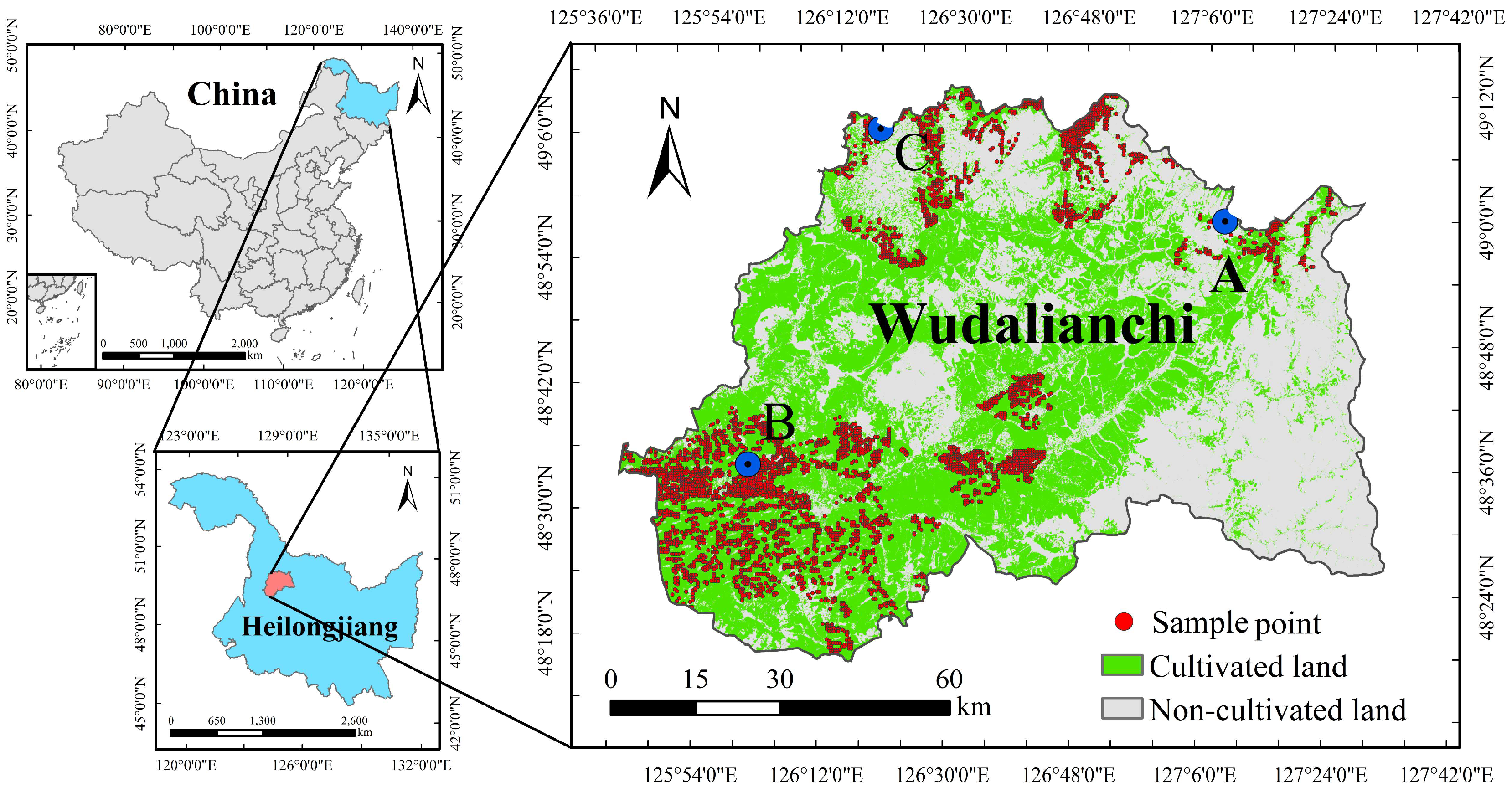[39] used random forest, BP neural networks, and other machine learning models to predict the application level of phosphorus fertilizer in different growth stages of crops. Applying artificial intelligence algorithms to the fertilization decision process can effectively improve the accuracy and universality of fertilization schemes. However, most of these studies focus on monitoring and predicting crop growth and soil nutrients using artificial intelligence methods without further attention on the relationship between fertilization management and crop yield. Therefore, this study conducted field sampling and lab measurements in Wudalianchi City, located in Heilongjiang Province, China, to establish a dataset and construct a fertilization decision model based on machine learning and swarm intelligent search algorithms. The purpose of this study is to (1) comprehensively use multiple machine learning algorithms to construct models for maize, rice, and soybean to improve the method of building a regression relationship between the fertilizer application rates and crop yield based on soil nutrients, fertilizations, and observed yield data; (2) evaluate the performance of different ML models for yield prediction; and, most importantly, (3) establish a fertilization decision model and provide references for the basic fertilizer application based on coupling the swarm intelligence algorithm and the selected ML model.

The remainder of the paper is structured as follows. Section 2 introduces an overview of the study area, the data collection procedure, and the basic theories and procedures of the yield prediction model and fertilization decision model. Section 3 analyzes the current soil nutrients, fertilization, and crop yields of the study area and evaluates the performance of different yield prediction models and the fertilization decision model. Section 4 discusses the rationality of recommended fertilization strategies, the comparison between the models in this study and others, and the improvement over the traditional STFF model. In Section 5, we summarize the superiority, insufficiency, and future improvements of this study.

2. Materials and Methods

2.1. Study Area

The study area is located in Wudalianchi City, Heilongjiang Province, China (48°42′00″ N, 126°35′30″ E). It covers an area of about 9900 km² and has a total population of about 170,000 people. Wudalianchi belongs to the cold temperate continental monsoon climate. The annual average temperature ranges from −3 to −1 °C, the average yearly precipitation is between 460 and 550 mm, the winter is cold and long, the annual frost-free period is about 110 days, the summer is hot and dry, and the annual sunshine duration exceeds 2500 h. Its sufficient water and climatic conditions, flat and open terrain, and fertile soil provide favorable conditions for agricultural development. The cultivated land area of the study area is about 0.4 million hectares, and the main food crops are soybean, maize, and rice (Figure 1). Given that Wudalianchi City is situated on the Northeast Plain of China, one of the country’s key grain-producing areas, the crop varieties and agricultural management practices are universal and typical. Additionally, excess fertilization is a severe issue in the surrounding area [40], so taking this place as a research object to improve fertilization management measures and increase crop yield can set a good example for other regions. Moreover, according to the basic geographical investigation of Wudalianchi City, we found that the cultivated land in this area is flat and open, covering a large area, which means it is possible to gather extensive crop data to employ machine learning techniques to simulate crop yield.

2.2. Data Collection

This study, in cooperation with the agricultural research personnel of the local Reclamation Bureau, conducted soil sampling on the cultivated plots of the three major crops of maize, rice, and soybean in Wulianchi City in April 2021 before crop seeding or transplanting. A total of 1634 fields (502 corn fields, 612 rice fields, and 564 soybean fields) were randomly selected for soil sampling, and 2–4 sampling points were set in each field along with crop type, field ID, field area, and coordinate information. More than five thousand soil samples at soil depth of 0–20 cm were collected in the study area (Figure 1). The soil pH, organic matter (OM), hydrolyzable nitrogen (HN), available phosphorus (AP), and available potassium (AK) were measured for all samples. Among them, OM was measured by the external heating potassium dichromate volumetric method [41]; pH was measured by an electronic pH meter (PH848, Smart Sensor, Ltd., Dongguan, China) (soil: water = 1:5); HN was measured by the alkaline hydrolysis diffusion method [41]; AP was measured using 0.5 mol/L sodium bicarbonate leaching combined with a molybdenum antimony anti-colorimetric process [42]; and after leaching with 1 mol/L ammonium acetate, AK was measured by flame photometry (FP640, Juchuang Group Co., Ltd., Qingdao, China) [42]. By averaging the data of the sample points with the same field ID, we obtained the characteristics of soil nutrients for the three main crops of maize, rice, and soybean in Wudalianchi City at the field scale. After the basic fertilizer was applied, farmers were surveyed about fertilizer amount, type, and other information by local Reclamation Bureau staff for further agricultural management, and we collected the fertilization data of relevant fields by retrieving agricultural management information using field ID with the help of the Reclamation Bureau in May 2021. Based on the fertilizer amount and main composition content information, we figured out the nitrogen (N), phosphorus (P₂O₅), and potassium (K₂O) application rate for the selected fields. We conducted regional surveys in the sampling fields with agricultural investigators who were responsible for crop yield investigations and local farmers to collect crop yield per unit for each field ID after the three main crops were harvested in October 2021.

2.3. Machine Learning Models

2.3.1. Random Forests

Random forest (RF), first proposed by Breiman [43], is a widely used machine learning model that introduces the idea of randomness into bagging (bootstrap aggregating). Specifically, RF uses the decision tree constructed based on the CART algorithm [44] as the base learner. Each base learner can randomly select samples from the original dataset with a replacement, create subsets, and then make classification (regression) rules according to the characteristics of the samples. Several essential learners jointly form the random forest and determine the prediction result by voting (average). Compared with the bagging method, the randomness of RF is reflected in two aspects. First, the process of selecting sub-datasets using RF is random, the samples in different sub-datasets can be repeated, and the samples in the same sub-dataset can also be repeated and second, in the splitting process of the decision tree node, RF will randomly select several features from all the features and then select the optimal feature from them, which can ensure the diversity of the entire system (Figure 2). More details about RF can be seen in the work of Breiman [43].

2.3.2. Extremely Randomized Trees

Extremely randomized trees (ERTs) is another machine learning model based on the decision tree method [45]. Similar to RF, ERT uses several decision trees as base learners for parallel computation and finally jointly decides the prediction result. However, ERT employs a more aggressive strategy in building decision trees. RF uses the bagging method to randomly select samples from the original dataset to construct sub-datasets to train decision trees. In contrast, ERT uses all the original data when building a decision tree. In addition, when selecting the optimal feature for decision tree node splitting, ERT randomly selects a feature sub-dataset and randomly selects the value within the value range of each candidate feature instead of the best threshold point as the feature’s split threshold, and then uses the MSE to evaluate and select the optimal feature.

The stronger randomness significantly improves the computational efficiency of ERT, but it also increases the error of the basic learner, especially the variance, because it is difficult to directly approach the decision boundary, which leads to the loss of a single basic learner in the ERT model [46]. Therefore, parameter determination is vitally important to obtain accurate performance from ERTs. Other calculation processes of RET can be referred to as RF, and the structure of this model is basically the same as RF.

2.3.3. Extreme Gradient Boosting

Extreme gradient boosting (XGBoost) is an efficient and flexible new machine learning model based on the gradient boosting decision tree (GBDT) method. It was proposed by Chen and Guestrin [47]. It uses the Taylor expansion to obtain the second derivative as an independent variable and automatically utilizes the CPU’s multi-threaded parallel computing to improve computational efficiency. It builds an end-to-end boosting system based on the tree model (Figure 3) [48].

As a boosting algorithm, the key of XGBoost is that it introduces the objective function, OBJ, as the judgment standard and compares the objective function changes before and after the iteration to determine whether to add new nodes. The calculation formula for the objective function is given by Equation (1).

$$OB{J}^{(k)}={\displaystyle \sum _{i=1}^{n}L(y_i,{\widehat{y}}_i{}^{(k)})}+{\displaystyle \sum _{k=1}^K\Omega (f_k)}$$

(1)

In Equation (1), n is the number of samples and y_i is the actual value of the sample. It can be seen from the above formula that the model objective function consists of two parts, where L is the traditional loss function, which represents the difference between the predicted value of the model and the actual value; Ω is the regular term, which can reflect the complexity of the model. More details about XGBoost can be seen in the work of Chen and Guestrin [47].

2.3.4. Yield Prediction Model

The collected physical and chemical characteristics of the soil and fertilization data were used to construct a feature set for model training as the two deciding factors of the yield prediction model (YPM). More precisely, the N, P, and K fertilizer application rates were used as fertilization characteristics, and the soil pH, OM, HN, AP, and AK were used as soil nutrient characteristics. Both fertilization and soil nutrient characteristics are regarded as independent variables (IVs), and a total of 3 IV combinations (IVCs) were applied to the establishment of the yield prediction model (

Table 1. Establishment of the independent variable combinations (IVCs) of the yield prediction model. HN: hydrolyzable nitrogen; AP: available phosphorus; AK: available potassium; OM: organic matter.

IVC	Feature Set
	Fertilization Characteristics			Soil Nutrient Characteristics
V1	N	P2O5	K2O	HN	AP	AK
V2	N	P2O5	K2O	HN	AP	AK	OM
V3	N	P2O5	K2O	HN	AP	AK	OM	pH

).

Taking the yield of the three main crops in the study area in 2021 as the target value, three machine learning algorithms, namely RF, ET, and XGBoost, were used to construct a crop yield prediction model, and the original data samples (corn: 1521, rice: 1831, soybean: 1722) were divided into a training set and test set according to a ratio of 8:2. During model training, to reduce the over-fitting problem caused by the small amount of model training data, the five-fold cross-validation method was used to divide the model training set into smaller subsets, which were alternately used as the training set and the validation set. The eigenvalues were standardized before input into the model to avoid the influence of dimension or magnitude differences among different eigenvalues on the index weight. The Bayesian optimization method [49] was first used to adjust the parameters within a given range, and then the parameters were manually optimized slightly. The parameters adjusted in RF and ERT include n_estimators, max_depth, min_samples_leaf, min_samples_split, and max_features. The parameters adjusted by XGBoost include n_estimators, learning_rate, max_depth, gamma, reg_lambda, min_child_weight, and sub_sample.

2.4. Swarm Intelligence Algorithm

2.4.1. Cuckoo Search Algorithm

The cuckoo search algorithm (CSA) is one of the classic swarm intelligence algorithms first proposed by Yang and Deb [50], which simulates the special breeding pattern of cuckoo parasitic chicks. In the iterative process, a new solution is generated to replace the poor solution through a random search, and at the same time, the generated new solution is discarded with a certain probability to gradually optimize the model results. The parameters to be adjusted are relatively few and the robustness is strong; thus, it has a wide range of applicability. (Equation (2)).

$$x_i^{(t+1)}=x_i^{(t)}+{\alpha }_{\mathrm{s}}\odot L(s,\lambda ), i=1,2,\cdots ,n$$

(2)

In Equation (2), x_i^(t) and x_i^(t+1) are the positions of the i^th bird’s nest in the t^th generation and the (t + 1)^th generation, respectively, ⊙ is the element-wise product, and L(s, λ) is the random search vector obeying the Levy distribution. Since the CSA uses the Lévy flights method [51] to find the optimal solution during iteration, combining a local dense random walk with a smaller step size and a global exploratory random walk with a larger step size can effectively expand the search range to avoid getting stuck in locally optimal solutions. The specific flow of the CSA to optimize the parameters is shown in Figure 4.

2.4.2. Fertilization Decision Model

The fertilization decision model (FDM) is established by coupling the selected YPM with the CSA. Precisely, the soil’s physical and chemical characteristics were fixed in the YPM model, and the amounts of N, P₂O₅, and K₂O were regarded as the variables to be optimized in the YPM model. The CSA was applied to optimize the amounts of N, P₂O₅, and K₂O to obtain the highest predicted crop yield of YPM.

After FDM was established, this study applied the stratified random sampling method to randomly select 100 sample points in each of the 3 crops to evaluate the performance of the FDM. More precisely, the optimal variables of each sample were used as inputs, while the population size, switching probability, and iteration number of the CSA were set as 25, 0.25, and 300, respectively.

2.5. Statistical Evaluation

The statistical index of coefficient of determination (R²), root mean square error (RMSE), mean absolute error (MAE), relative root mean square error (RRMSE), and mean absolute percentage error (MAPE) were used to evaluate the model’s performance (Equations (3)–(7)).

$$R^2=1-\frac{{\displaystyle \sum _{i=1}^n{\left({\widehat{y}}_i-y_i\right)}^2}}{{\displaystyle \sum _{i=1}^n{\left({\overline{y}}_i-y_i\right)}^2}}$$

(3)

$$RMSE=\sqrt{\frac{1}{n}{\displaystyle \sum _{i=1}^n{\left({\widehat{y}}_i-y_i\right)}^2}}$$

(4)

$$MAE=\frac{1}{n}{\displaystyle \sum _{i=1}^n\left|\left({\widehat{y}}_i-y_i\right)\right|}$$

(5)

$$RRMSE=\frac{\sqrt{\frac{1}{n}{\displaystyle \sum _{i=1}^n{\left({\widehat{y}}_i-y_i\right)}^2}}}{\sqrt{\frac{1}{n-1}{\displaystyle \sum _{i=1}^n{\left({\overline{y}}_i-y_i\right)}^2}}}$$

(6)

$$MAPE=\frac{1}{n}{\displaystyle \sum _{i=1}^n\left|\frac{{\widehat{y}}_i-y_i}{y_i}\right|}\times 100\%$$

(7)

In Equations (3)–(7), y_i, ŷ_i, and ${\overline{y}}_i$ are the observed, predicted, and averaged values, respectively. n is the number of samples. The larger R² and smaller MAE, RMSE, RRMSE, and MAPE indicate higher accuracy.

3. Results and Analyses

3.1. Analysis of Soil Characteristics, Fertilization, and Crop Yield

The soil characteristics of samples in the study area are indicated in

Table 2. Descriptive statistical analysis of soil characteristics at sampling sites. HN: hydrolyzable nitrogen; AP: available phosphorus; AK: available potassium; OM: organic matter.

Item	Minimum	Maximum	Mean	STD	CV	Skewness	Kurtosis
					%	-	-
pH	4.61	8.16	6.23	0.74	11.84	0.55	0.32
HN	54.10	612.40	195.68	58.95	30.12	0.85	1.69
AP	3.40	200.00	45.21	24.51	54.20	0.89	1.13
AK	45.00	491.00	195.36	57.18	29.27	0.76	1.07
OM	10.30	164.00	49.13	15.20	30.93	1.80	5.47

The units for HN, AP, and AK are mg kg⁻¹, while the unit for OM is g kg⁻¹.

. The average soil pH was 6.23, which was weakly acidic. The coefficient of variation (CV) of soil characteristics for the samples was between 10% and 100%, which represents a medium variation. The CV of OM, HN, and AK was relatively small (about 30%), indicating that the spatial distribution was relatively stable. The CV of AP was greater than 50%, showing a relatively high degree of spatial dispersion. The skewness and kurtosis values of soil nutrient contents (HN, AK, and AP) were larger than 0.5, which represented a positively skewed distribution. According to the specification for geochemical evaluation of land quality in Northeast China (

Table 3. Soil nutrient classification of typical black soil areas in Northeast China. HN: hydrolyzable nitrogen; AP: available phosphorus; AK: available potassium; OM: organic matter.

Level	HN	AP	AK
	mg kg−1
Very rich	>150	>40	>200
Rich	120–150	20–40	150–200
Moderate	90–120	10–20	100–150
Deficient	60–90	5–10	50–100
Very deficient	30–60	3–5	30–50
Extremely deficient	<30	<3	<30

) [52], HN and AP content of the soil in the study area is very rich, and AK is at the upper limit of the rich level.

The application rates of N, P₂O₅, and K₂O for collected samples are shown in

Table 4. Descriptive statistical analysis of application rates of N, P₂O₅, and K₂O for the maize, rice, and soybean sampling sites.

Crop	Fertilizer	Minimum	Maximum	Mean	STD	CV	Skewness	Kurtosis
		kg ha−1				%	-	-
Maize	N	33.8	265.4	100.6	31.4	31.17	1.88	2.83
	P2O5	22.9	169.1	72.5	15.7	19.04	−0.43	3.17
	K2O	33.8	170.0	80.5	26.6	28.43	4.88	28.63
Rice	N	36.0	257.2	158.3	20.1	22.75	0.68	0.69
	P2O5	24.7	90.0	64.5	21.6	33.53	−0.74	−0.99
	K2O	36.0	170.0	112.6	53.6	47.60	0.89	−0.86
Soybean	N	31.5	96.7	51.9	12.2	29.01	5.79	40.64
	P2O5	26.8	127.0	87.6	6.1	16.07	4.30	29.17
	K2O	31.5	225.0	62.6	18.4	43.20	7.14	58.48

. The CV of fertilization for these three major crops was between 10% and 100%, indicating a medium variation in the overall picture. However, the CV of the N application rates for maize, P₂O₅, and K₂O application rate for rice, and the K₂O application rate for soybean was greater than 30%, which shows the relatively high spatial variability of these fertilizers in different fields. Furthermore, we noted that the minimum (maximum) values of fertilizer application rates for crops were extremely low (high) compared with the recommended dosages from published papers [53,54,55], indicating highly unreasonable fertilization in some fields.

The relationship between the normalized HN, AP, and AK contents and the application rates of N, P₂O₅, and K₂O for maize, rice, and soybean are indicated in Figure 5. The absolute values of the range of HN content for maize, rice, and soybean were 55.6–612.4 mg kg⁻¹, 76.5–333.1 mg kg⁻¹, and 78.8–508.5 mg kg⁻¹. Similarly, the absolute values of the range of AP and AK for maize, rice, and soybean were 3.4–134.8 mg kg⁻¹, 9.8–200.0 mg kg⁻¹, 5.0–193.4 mg kg⁻¹, 45.1–491.2 mg kg⁻¹, 86.4–463.2 mg kg⁻¹, and 83.7–462.1 mg kg⁻¹. However, in order to compare the changes in fertilization of these three crops under different soil nutrient conditions, all fertilization and soil nutrient data were normalized. It is known that crops absorb required nutrients from both soil and fertilizer during the growth stage, so the original nutrient supply capacity of soil in different fields should be considered when deciding the fertilization formula. The amount of fertilizer should be reduced appropriately in the soil with high N, P, and K content, and more fertilizer should be applied in the field with relatively low nutrient content. Since soil nutrients in this region were at a high level, the application rates of N, P₂O₅, and K₂O should have decreased with the increase in soil nutrient content. However, it can be seen that under the current fertilization conditions, the application rates of N, P₂O₅, and K₂O did not match the soil nutrient content of the field. There was little difference in the amount of fertilization at different relative soil nutrient content intervals. Specifically, with the increase in soil HN content, the average N application rate of rice first increased and then decreased. When the soil HN content was 0.2–0.4, the average N application rate of rice was the largest (0.65); the average N application rate of maize and soybean fluctuated around 0.26 and 0.08, respectively. The average P₂O₅ application rate of rice decreased with the fluctuation of soil AP content, and the maximum P₂O₅ application rate (0.71) appeared in the range of AP content from 0–0.2; the average P₂O₅ application rate of maize and soybean fluctuated around 0.40. With the increase in soil AK content, the average K₂O application rate of maize showed a fluctuating upward trend, and the maximum value was 0.54 when the soil AK content ranged from 0.2 to 0.4; the average K₂O application rate of rice and soybean fluctuated around 0.05.

The above analysis proved that the current fertilizer application schedules were inappropriate in the study area. Moreover, the inappropriate fertilizer application schedules have caused crop yield reductions. Taking location A in Figure 1 as an example, the contents of HN, AP, and AK in the soil were in the top 35.1%, 18.2%, and 7.4% of the overall soil nutrient content (

Table 5. Soil nutrient contents and corresponding amounts of actual fertilization in the sample points. HN: hydrolyzable nitrogen; AP: available phosphorus; AK: available potassium; OM: organic matter.

Sample Point	Crop	HN	AP	AK	N	P2O5	K2O	Yield
		mg kg−1			kg ha−1
A	Maize	235.9	67.3	277	103.7	77.1	82.2	5160
B	Rice	99.3	10.1	106	91.7	63.7	78.8	6380
C	Soybean	179.3	23.4	162	48.3	30.2	36.8	2146

), respectively, proving that the original soil fertility was relatively high in this location. Reducing the application amount of the corresponding fertilizer should be considered to avoid excessive fertilization. However, the actual application rates of N, P₂O₅, and K₂O were in the top 24.8%, 8.9%, and 21.1% of the total, which were all at a relatively high level, resulting in the maize yield of this location being only 58.7% of the average yield. In contrast, the soil HN, AP, and AK contents at location B (Figure 1) were only in the top 98.6%, 99.8%, and 96.4% of the overall soil fertility (Table 5), respectively, and the soil fertility was relatively low. Meanwhile, the actual application rates of N, P₂O₅, and K₂O were only in the top 88.9%, 50.2%, and 91.5% of the overall fertilization amount, respectively, resulting in only 83.4% of the average rice yield.

Similarly, the contents of HN, AP, and AK at location C (Figure 1) were in the top 55.4%, 77.4%, and 67.5% of the overall soil nutrient content, respectively (Table 5), while the application rates of N, P₂O₅, and K₂O were only in the top 96.4%, 95.5%, and 96.6%, indicating the amounts of fertilization were very low and resulting in the soybean yield of location C being only 75.7% of the average. Therefore, the current fertilizer application rates in the study area do not consider the actual growth needs of crops and basal soil fertility, resulting in a big difference between the actual crop yield and the expected yield.

3.2. Performance of the Machine Learning Models for Yield Prediction

3.2.1. Random Forest Model

The actual yields of maize, rice, and soybean were divided into eight intervals and noted as M1–M8, R1–R8, and S1–S8, respectively, which could better reflect the crop yield distribution and reduce the influence of random error caused by the field survey (Figure 6). It can be seen that the predicted yield of different crops in each interval is close to the actual value. However, there are still specific differences among the three crops using different IVCs (

Table 6. Statistical evaluations of predicted yields of maize, rice, and soybean based on the RF model.

Crop	Feature Set	Evaluation Indices
		R2	RMSE	MAE	RRMSE	MAPE
		kg ha−1			-	%
Maize	V1	0.468 (0.034)	997.7 (57.0)	737.6 (58.9)	0.098 (0.007)	7.970 (0.912)
	V2	0.524 (0.042)	944.0 (58.4)	700.0 (58.6)	0.093 (0.007)	7.587 (0.718)
	V3	0.557 (0.047)	910.0 (56.9)	656.0 (64.4)	0.090 (0.007)	7.161 (0.907)
Rice	V1	0.695 (0.061)	420.3 (38.7)	318.8 (39.4)	0.056 (0.005)	4.240 (0.486)
	V2	0.727 (0.058)	401.7 (46.3)	313.1 (41.1)	0.054 (0.005)	4.221 (0.339)
	V3	0.749 (0.068)	406.7 (39.4)	310.6 (40.8)	0.054 (0.006)	4.198 (0.563)
Soybean	V1	0.604 (0.032)	189.4 (22.7)	143.5 (13.7)	0.084 (0.008)	6.447 (0.602)
	V2	0.627 (0.069)	183.8 (23.2)	136.9 (10.3)	0.081 (0.008)	6.150 (0.564)
	V3	0.634 (0.059)	181.9 (23.4)	134.9 (16.6)	0.080 (0.008)	6.073 (0.640)

The standard deviations of each index are added in parentheses.

). RF obtained the highest accuracy for rice yield prediction when the IVC was V3.

In addition, the yield prediction accuracy of the three crops using different IVCs showed the same rule, namely V3 > V2 > V1. Specifically, when using V3 for maize yield prediction, the R² was increased by 19.13% and 6.44% compared with V1 and V2, respectively, and the RRMSE was relatively reduced by 8.80% and 3.61%. The R² of the predicted rice and soybean yields increased by 12.87%, 3.06%, 5.08%, and 1.21%, and the RRMSE decreased by 8.29%, 1.31%, 3.95%, and 1.02%, respectively. Therefore, using pH, OM, HN, AP, and AK to predict crop yield can improve prediction accuracy. Further comparison found that the R² of maize, rice, and soybean when using V3 for yield prediction were 0.577, 0.739, and 0.634, respectively, and the order from large to small was rice > soybean > maize; while the RMSE and MAPE were 0.090, 0.055, 0.080, and 7.161%, 4.258%, and 6.073%, respectively, and the order from small to large was rice < soybean < maize. The standard deviations of the evaluation indexes for RF were relatively small and the ratios of the standard deviation to the mean were generally distributed between 0.05 and 0.13, which indicated the stable prediction of the model. Furthermore, the standard deviations decreased slightly when using V1 for prediction, and the variability of the yield prediction model for maize is the smallest. In summary, it can be seen that the RF model has the highest accuracy for rice yield prediction, followed by soybean and maize.

3.2.2. Extremely Randomized Trees

Similar to RF, ERTs also obtained the highest prediction accuracy with V3 (Figure 7). Compared with the use of V2 and V1, using V3 increased the R² of maize, rice, and soybean by 21.34%, 12.04%, 6.89%, and 6.64%, 4.79%, and 4.41%, respectively. In comparison, the RRMSE decreased by 10.97%, 9.92%, 5.61%, 4.29%, 1.98%, and 3.78%, respectively. Meanwhile, the rice yield prediction accuracy of the ERT model was still the highest among the three crops. Comparing the results of yield prediction using V3, it can be found that the R² of maize, rice, and soybean were 0.598, 0.775, and 0.655, respectively, while the MAPE and RRMSE were 0.086, 0.051, 0.078, and 6.792%, 3.906%, and 5.828%, respectively (

Table 7. Statistical evaluations of predicted yields of maize, rice, and soybean based on the ERT model.

Crop	Feature Set	Evaluation Indices
		R2	RMSE	MAE	RRMSE	MAPE
		kg ha−1			-	%
Maize	V1	0.493 (0.054)	974.1 (125.9)	737.4 (67.3)	0.096 (0.007)	7.998 (0.748)
	V2	0.561 (0.080)	906.2 (93.8)	672.6 (71.8)	0.089 (0.007)	7.337 (0.819)
	V3	0.598 (0.081)	867.3 (116.1)	619.6 (73.5)	0.086 (0.009)	6.792 (0.919)
Rice	V1	0.692 (0.063)	425.1 (50.5)	312.6 (37.7)	0.057 (0.006)	4.331 (0.572)
	V2	0.740 (0.052)	390.7 (54.5)	287.3 (42.3)	0.052 (0.006)	3.957 (0.449)
	V3	0.775 (0.104)	386.9 (55.7)	287.4 (43.8)	0.051 (0.006)	3.902 (0.553)
Soybean	V1	0.655 (0.059)	176.7 (17.2)	129.5 (12.7)	0.078 (0.009)	5.828 (0.610)
	V2	0.627 (0.057)	183.6 (21.1)	137.5 (17.3)	0.081 (0.009)	6.173 (0.598)
	V3	0.655 (0.078)	176.7 (20.8)	129.5 (16.3)	0.078 (0.010)	5.828 (0.591)

The standard deviations of each index are added in parentheses.

). The ratios of the standard deviation to the mean were about 0.05 to 0.15, which were a little higher than RF, and the model for maize was the most stable. The prediction accuracy of the ERT model for the three crop yields from high to low was rice > soybean > maize.

3.2.3. Extreme Gradient Boosting

Yield predictions of maize, rice, and soybean using XGBoost are shown in

Table 8. Statistical evaluations of predicted yields of maize, rice, and soybean based on the XGBoost model.

Crop	Feature Set	Evaluation Indices
		R2	RMSE	MAE	RRMSE	MAPE %
		kg ha−1			-	%
Maize	V1	0.480 (0.036)	986.0 (94.1)	715.3 (64.3)	0.097 (0.006)	7.690 (0.549)
	V2	0.540 (0.038)	927.4 (90.7)	691.7 (78.3)	0.091 (0.008)	7.428 (0.865)
	V3	0.545 (0.047)	922.4 (93.2)	659.4 (71.1)	0.091 (0.008)	7.182 (1.063)
Rice	V1	0.692 (0.095)	425.1 (32.9)	309.3 (28.8)	0.057 (0.007)	4.265 (0.253)
	V2	0.724 (0.107)	402.2 (42.9)	284.8 (30.5)	0.054 (0.007)	3.917 (0.368)
	V3	0.744 (0.112)	412.7 (56.7)	312.4 (29.9)	0.055 (0.008)	4.206 (0.388)
Soybean	V1	0.589 (0.059)	192.9 (22.1)	145.2 (11.4)	0.085 (0.009)	6.533 (0.683)
	V2	0.604 (0.057)	189.2 (26.2)	142.2 (12.3)	0.083 (0.009)	6.348 (0.475)
	V3	0.622 (0.068)	185.1 (28.1)	136.8 (19.6)	0.082 (0.009)	6.120 (0.696)

The standard deviations of each index are added in parentheses.

. Similar to RF and ERT, using V3 as input variables obtained the highest accuracy in yield prediction. However, the improvements of V3 in XGBoost compared with V1 and V2 were smaller than in RF and ERT. In XGBoost, the use of V3 increased the R² for maize, rice, and soybean by 13.54%, 7.51%, and 5.60% compared to V1, and by 0.93%, 2.76%, and 2.98% compared to V2, respectively. The change in RRMSE was even more minor. When using V3 to predict yield, the RRMSE of maize decreased by 6.19% compared with V1 and V2; the RRMSE of rice decreased by 3.51% compared with V1 but increased by 1.85% compared with V2; the RRMSE of soybean was reduced by 3.53% and 1.20% compared with V1 and V2, respectively. With V3, XGBoost obtained the highest accuracy for rice, followed by soybean and maize, which were also similar to RF and ERT. Specifically, the R² of maize, rice, and soybean was 0.545, 0.744, and 0.622, respectively, and the RRMSE and MAPE were 0.091, 0.055, 0.082, and 7.182%, 4.206%, and 6.120%, respectively (Figure 8). The range of ratios of the standard deviation to the mean was between 0.07 and 0.16, which was the highest among the three models, and the dispersion of maize was the smallest.

3.2.4. Determining the Best Machine Learning Model for Yield Prediction

The above analysis indicated that using V3 as input variables obtained the highest accuracy for yield prediction for all three ML models. Moreover, the accuracy order of the three crops was rice, soybean, and maize in all three ML models. The ERT model had the largest R² and lowest MAPE for maize, rice, and soybean, which proved to have the highest accuracy among these three models. Regarding the robustness of the models, there was little difference between RF, ERT, and XGBoost since the ratios of the standard deviation to the mean of the indexes were basically the same, and the standard deviations of ERT were small enough. Therefore, ERT with features of HN, AP, AK, OM, and pH was determined as the best ML model for yield prediction. It was coupled with the CSA to establish the fertilization decision model with the hyperparameters in

Table 9. Optimized hyperparameters of the ERT model for yield prediction of maize, rice, and soybean.

Crop	Hyperparameter	Range	Bayesian Optimization	Manual Optimization
Maize	n_estimators	(400, 800)	450	450
	max_depth	(5, 30)	15	16
	min_samples_leaf	(1, 20)	1	1
	min_samples_split	(2, 20)	6	6
	max_features	(2, 7)	6	5
Rice	n_estimators	(400, 800)	550	560
	max_depth	(5, 30)	20	21
	min_samples_leaf	(1, 20)	1	1
	min_samples_split	(2, 20)	6	6
	max_features	(1, 7)	6	6
Soybean	n_estimators	(400, 800)	450	450
	max_depth	(5, 30)	20	22
	min_samples_leaf	(1, 20)	1	1
	min_samples_split	(2, 20)	5	5
	max_features	(1, 7)	6	6

.

As an ensemble model based on a decision tree algorithm, the ERT model uses Gini Importance (GI) and Permutation Importance (PI) as two main indicators to characterize feature importance [43,56]. The GI was calculated by evaluating all nodes’ average impurity reduction ranks in the feature division processes. The PI was to randomly shuffle the arrangement order of a particular eigenvalue and then recalculate the model’s prediction performance.

Regardless of whether GI or PI was used, the N application rates of the three crops were the essential characteristics of the ERT model, which were around 0.25 (GI) and 0.23 (PI), respectively. The second and third were P₂O₅ and K₂O application rates, respectively (Figure 9). Therefore, the amount of fertilizer applied was an essential factor affecting crop yield, and using scientific and reasonable fertilization ratios might effectively improve crop yield.

3.3. Performance of the Fertilization Decision Model

The performance of the CSA has been verified in many earlier studies [57,58,59,60]. In particular, its parameter optimization effect was significantly improved compared with other optimization algorithms, such as particle swarm optimization and differential evolution algorithms. In the current study, the FDM updates the application rates of N, P₂O₅, and K₂O using the CSA to maximize the crop yield predictions with ERT. After the calculation of the FDM, the recommended fertilizer formula (RFF) and the predicted yields in the RFF are available, and the comparison between predicted and observed yields is indicated in

Table 10. Comparison between predicted yields calculated by the FDM and observed yields.

Crop	Max	Type	Best	Worst	Mean	STD
			kg ha−1
Maize	11,250	Simulation	11,205	10,665	10,875	120.63
		Observation	11,250	6750	8790	1321.23
Rice	9000	Simulation	8985	8415	8655	119.12
		Observation	9000	6300	7650	706.55
Soybean	4050	Simulation	3597	3208	3410	97.37
		Observation	4020	1725	2835	351.45

.

The results indicated that the RFF could significantly improve crop yields. Assuming that soil nutrient content remains constant and the fertilization formula of each field is optimized, the predicted average yields of maize, rice, and soybean are 23.9%, 13.3%, and 20.3% higher than the observed values, respectively, which are 96.8%, 96.3%, and 84.1% of the maximum yields of the maize, rice, and soybean in the survey. In addition, the distribution of the three crop-predicted yield values after CSA optimization is shown in Figure 10. More than 75% of the predicted values reached 96.1%, 95.5%, and 82.4% of the maximum value, respectively. Moreover, the standard deviations (STDs) of predicted maize, rice, and soybean yields were all not more than 150 kg ha⁻¹, showing strong stability of the FDM under different crops and soil fertility conditions.

4. Discussion

The Northeast region, including Heilongjiang, is one of the essential grain-producing areas in China. Many researchers have conducted quantitative research on the appropriate amount of fertilization for the main crops in this region. Wu et al. [61] proposed that the recommended N, P₂O₅, and K₂O application rates for maize were 150–188 kg ha⁻¹, 75–97 kg ha⁻¹, and 57–60 kg ha⁻¹, respectively. Wu et al. [53] also indicated that the suitable N, P₂O₅, and K₂O application rates for rice were 116–156 kg ha⁻¹, 64–70 kg ha⁻¹, and 45–59 kg ha⁻¹, respectively. Based on field experiments, Ji et al. [54] found that the optimal N, P₂O₅, and K₂O application rates for maize in Heilongjiang were 176–180 kg ha⁻¹, 65–70 kg ha⁻¹, and 75–90 kg ha⁻¹, respectively. The experimental study by Kong et al. [55] showed that the optimal N application rate for rice in Heilongjiang was 112.3–150 kg ha⁻¹, while the optimal P₂O₅ and K₂O application rates were 46.7–63.1 kg ha⁻¹ and 38.3–57.5 kg ha⁻¹, respectively. Sun et al. [19] carried out soil testing and formula fertilization experiments and believed that the optimal N application rate for soybeans in the medium soil fertility area of Heilongjiang was 28.4–36.3 kg ha⁻¹, and the optimal P₂O₅ and K₂O application rates were 38.9–47.7 kg ha⁻¹ and 43.2–51.2 kg ha⁻¹, respectively.

Based on the ratio of base fertilizer and topdressing fertilizer recommended in previous studies [19,53,61], the recommended fertilization formula ranges of the FDM for the 100 selected fields are shown in

Table 11. Statistics of the recommended fertilization amounts for maize, rice, and soybean.

Crop	N Application			P Application			K Application
	Min	Max	Mean	Min	Max	Mean	Min	Max	Mean
	kg ha−1
Maize	133.7	240.4	178.6	63.1	91.2	75.5	46.4	112.6	67.1
Rice	111.1	162.2	142.3	37.5	79.1	48.7	37.2	79.5	57.4
Soybean	37.2	57.1	43.3	55.7	105.1	70.2	42.0	73.3	54.2

. The recommended application ranges of N, P₂O₅, and K₂O for maize were 133.5–240.0 kg ha⁻¹, 63.0–91.5 kg ha⁻¹, and 46.5–112.5 kg ha⁻¹, respectively. The recommended fertilizer rates for rice and soybean were 111.0–162.0 kg ha⁻¹, 37.5–79.5 kg ha⁻¹, 46.5–79.5 kg ha⁻¹, and 37.5–57.0 kg ha⁻¹, 55.5–105.0 kg ha⁻¹, and 46.5–73.5 kg ha⁻¹, respectively. Therefore, the recommended fertilization amount of the FDM constructed in this study was consistent with the previous research for maize, rice, and soybean in Heilongjiang. Meanwhile, we also found that the recommended fertilization range of the FDM was generally wider than in the previous studies. The main reason was that the FDM provides personalized fertilization plans based on the original soil fertility of different fields. The recommended fertilization rate will be much higher or lower than the average level in areas with significantly low or high soil fertility. Therefore, the FDM constructed in this study can provide stable and high-yield fertilization formulas based on the soil’s physicochemical properties in different fields, especially in the base fertilizer application stage. However, further and more detailed exploration is required for the fertilization management plan for the whole process of the crop growth period.

Compared with the traditional STFF, the FDM proposed in this study has the advantage of eliminating tedious field fertilization experiments and quickly and easily offering crop fertilization formulas. It is because the traditional STFF, whether the nutrient balance method or the fertilizer effect method, requires field trials during the entire growth period of crops, which is time-consuming and lacks universality. For example, Tong et al. [62] tried to explore the optimal nitrogen, phosphorus, and potassium fertilization ratios for maize in Heilongjiang with the fertilizer effect method. However, it took 129 days to set up the experiments with 14 treatments and 5 repetitions in a 700 m² maize field. Li et al. [42] constructed the STFF model of broccoli based on effective functions of P, N, and K for broccoli yield, which needed a one-month field experiment with eleven fertilization treatments with three repetitions in thirty-three plots. Different from the above studies, to construct the FDM, all we need are historical soil nutrient parameters, fertilization rates, and yield data, which are becoming more and more convenient to obtain thanks to the development of modern agricultural management systems. On the premise of ensuring accuracy, the use of artificial intelligence methods to construct the model saves a lot of manpower and material resources and improves the efficiency of formula fertilization. Traditional statistical methods and data processing techniques have been unable to meet the needs of agricultural production for efficient extraction of valuable information from field data during the rapid development of agricultural digitalization [63]. Machine learning methods, on the other hand, can directly use experience and follow specific learning rules to train data to mine complex nonlinear relationships between input variables such as agricultural environment, management measures, crop phenotypes, and predictor variables to accurately and conveniently solve problems such as crop yield forecasting, soil management, and other agricultural practical issues [33,64]. However, with the advantages come some new challenges compared with traditional STFF. For example, to build an STFF model with good performance and robustness based on artificial intelligence methods, a large amount of crop data from many diverse environments and management scenarios is required. Additionally, a lot of effort must put into data preprocessing to improve the quality of the data and make sure the dataset is representative.

Some researchers have also tried to use ML models to recommend crop fertilization rates and construct the response relationship between soil parameters, weather, and other factors and fertilization rates. ML is a reasonable method for constructing a regression relationship between a list of variables and the target value with tabular data, and may even be better than deep learning (DL) [48]. However, some of them were relatively complex and difficult to apply in practice. For example, Bean et al. [65] built a N fertilizer rate recommendation model using a large number of parameters that need to be adjusted and included many variables that are difficult to obtain, which cannot take into account accuracy and achievability together and lacks operability in actual agricultural management. Additionally, few studies have considered all three major fertilizers (N, P₂O₅, and K₂O) in the fertilization optimizations; most of them focused on one optimum fertilizer rate, ignoring the effects of different fertilizer combinations on crop growth [66,67]. In contrast, the FDM constructed in this study only considers the environmental factors most directly related to the fertilization process and is based on soil nutrients to give the fertilization formula for all three major crops of maize, rice, and soybean, which have greater practicality. The recommended ratio of N, P, and K is also provided to increase the crop yield. In addition, the recommended fertilization rates of other studies cannot fully account for the spatial variability of different fields and only give an average fertilizer formula [18]. However, fertilizer requirements for crops could vary with the change in physical position because of the spatial diversity of the original nutrients in the soil. Moreover, the FDM constructed in this study also considers the temporal and spatial differences in crop fertilizer demands and can provide specific fertilization formulas according to the crop types and soil nutrient content of different fields. This strategy has been proven by Rotundo et al. [68] to be efficient and valuable.

Finding the optimal fertilization rate parameters based on the CSA is another crucial point in constructing the FDM. As a recognized meta-heuristic algorithm, the CSA can effectively solve various optimization problems. The most significant advantage of the CSA is that it better balances accuracy and achievability, and the search strategy combining a local search and global search ensures that the algorithm has excellent performance and only needs to configure a small number of parameters to deal with complex multi-objective problems [69]; thus, it is widely used in optimization problems in image processing, medical, data mining, power energy, engineering design, and other fields [70]. The combination of the CSA and ML is an effective method to improve the efficiency of solving optimization problems. When using ML to predict complex nonlinear problems, the CSA can optimize the hyperparameters that need to be manually set in the ML process and improve the efficiency and accuracy of the simulation.

The CSA-SVM (support vector machine) model constructed by Zhang et al. [71] is a typical representation of this application in short-term electrical load forecasting; he used the CSA to optimize the two primary hyperparameters of the SVM model with different forecasting strategies to improve the prediction accuracy of the SVM. Guo et al. [72] introduced the CSA into the optimization process of the number of decision trees and nodes in RF and applied it to the parameter prediction of geotechnical engineering, significantly reducing the prediction error. To obtain fertilization strategies, previous studies [19,73,74] usually divided soil nutrients into different levels based on relative crop yields manually before constructing the fertilizer response equation, and then retrieved suitable fertilization according to the optimal yield of different soil nutrient levels. The procedures for soil nutrient level division were relatively rough and subjective, and the regression equation for fertilization and crop yields had poor accuracy. In this study, the combination of the CSA and ML is used, that is, after building a crop yield prediction model based on ERT, in the case of known field soil nutrient parameters as part of the input, with the maximum yield as the optimization goal, the CSA is used to search for the best N, P₂O₅, and K₂O fertilizer application range. Compared to traditional STFF models, the FDM driven by the CSA could automatically seek the fertilization strategy that matches the soil nutrients to maximize crop yield, which is more convenient and accurate.

5. Conclusions

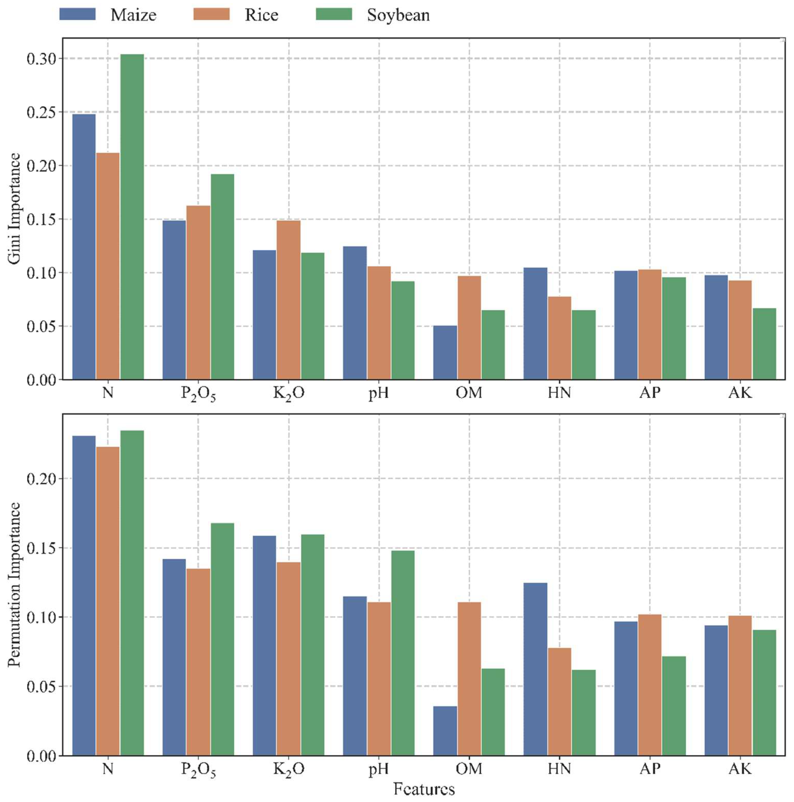
In this study, three machine learning models, including RF, ERT, and XGBoost, were used to predict the yield of maize, rice, and soybean with fertilization and soil nutrient characteristics. The results indicated that the ERT model with soil pH, OM, HN, AP, AK, and the fertilizers N, P₂O₅, and K₂O as inputs could obtain the highest accuracy of crop yield predictions. The R² and RRMSE of maize, rice, and soybean were 0.749, 0.775, 0.744, and 0.086, 0.051, and 0.078, respectively. In addition, the three most important variables were the application rates of N, P₂O₅, and K₂O.

After that, this study also coupled the CSA with ERT to establish the fertilization decision model (FDM) using the amounts of N, P₂O₅, and K₂O as independent variables to obtain the highest predicted yields of maize, rice, and soybean, respectively. The field survey data in Wudalianchi, Heilongjiang province, China, indicated that the proposed FDM could increase the yield of maize, rice, and soybean by 23.9%, 13.3%, and 20.3% compared with the average yield value in 2021. The FDM established in this study balanced accuracy and practicality and constructed a complex nonlinear relationship between fertilization and crop yields based on artificial intelligence algorithms with soil characteristics, which are relatively readily available environmental factors. It can provide a more convenient and efficient solution for large-scale regional fertilization management. Furthermore, on the premise of collecting sufficient historical crop data, the modeling process of this study can be reproduced in other regions. Fertilization decision models with different soil characteristics and crops can be easily established, which indicates a great potential for promotion.

As this is our first attempt at applying artificial intelligence algorithms to crop fertilization management, the quantity and time span of the collected crop data were limited, and the performance of the YPM remains to be improved. Since the main purpose of this paper was to explore a more effective way to construct the regression relationship between the fertilizer application rate and crop yield to replace the old methods in traditional STFF research, we did not take other environmental factors or economic benefits into consideration. In the future, by expanding the size of the model dataset and introducing more elements affecting crop growth, such as weather and terrain, the robustness and universality of the model will be improved. Additionally, more efforts should be put into the data preprocessing with the expansion of the data scale, such as data cleaning (filling in the missing values, wiping off the abnormal data, and smoothing the noise), feature dimension reduction and feature crosses, and data conversion (standardization and discretization). Moreover, deep learning models with a superior ability in data processing (e.g., LSTM, transformer) and multi-objective optimization involving economic benefits and crop yields could be used to build the FDM to improve the accuracy of fertilization decisions.

References

1. Timilsena, Y.P.; Adhikari, R.; Casey, P.; Muster, T.; Gill, H.; Adhikari, B. Enhanced Efficiency Fertilisers: A Review of Formulation and Nutrient Release Patterns: Enhanced Efficiency Fertilizers. J. Sci. Food Agric. 2015, 95, 1131–1142. [Google Scholar] [CrossRef] [PubMed]
2. Stewart, W.M.; Dibb, D.W.; Johnston, A.E.; Smyth, T.J. The Contribution of Commercial Fertilizer Nutrients to Food Production. Agron. J. 2005, 97, 1–6. [Google Scholar] [CrossRef]
3. Kharbach, M.; Chfadi, T. General Trends in Fertilizer Use in the World. Arab. J. Geosci. 2021, 14, 2577. [Google Scholar] [CrossRef]
4. Chen, X.; Ma, L.; Ma, W.; Wu, Z.; Cui, Z.; Hou, Y.; Zhang, F. What Has Caused the Use of Fertilizers to Skyrocket in China? Nutr. Cycl. Agroecosyst. 2018, 110, 241–255. [Google Scholar] [CrossRef]
5. Huang, S.W.; Tang, J.W.; Li, C.H.; Zhang, H.Z.; Yuan, S. Reducing Potential of Chemical Fertilizers and Scientific Fertilization Countermeasure in Vegetable Production in China. J. Plant Nutr. Ferti. 2017, 23, 1480–1493. [Google Scholar]
6. Xue, C.; Zhang, T.; Yao, S.; Guo, Y. Effects of Households’ Fertilization Knowledge and Technologies on Over-Fertilization: A Case Study of Grape Growers in Shaanxi, China. Land 2020, 9, 321. [Google Scholar] [CrossRef]
7. Zhao, Y.; Luo, J.-H.; Chen, X.-Q.; Zhang, X.-J.; Zhang, W.-L. Greenhouse Tomato–Cucumber Yield and Soil N Leaching as Affected by Reducing N Rate and Adding Manure: A Case Study in the Yellow River Irrigation Region China. Nutr. Cycl. Agroecosyst. 2012, 94, 221–235. [Google Scholar] [CrossRef]
8. Guo, Y.; Wang, J. Spatiotemporal Changes of Chemical Fertilizer Application and Its Environmental Risks in China from 2000 to 2019. Int. J. Environ. Res. Public Health 2021, 18, 11911. [Google Scholar] [CrossRef]
9. Hakl, J.; Kunzová, E.; Konečná, J. Impact of Long-Term Organic and Mineral Fertilization on Lucerne Forage Yield over an 8-Year Period. Plant Soil Environ. 2016, 62, 36–41. [Google Scholar] [CrossRef]
10. Pageau, D.; Lajeunesse, J.; Lafond, J. Effect of seeding rate and nitrogen fertilization on oilseed flax production. Can. J. Plant Sci. 2006, 86, 363–370. [Google Scholar] [CrossRef]
11. Fischer, G.; Winiwarter, W.; Ermolieva, T.; Cao, G.-Y.; Qui, H.; Klimont, Z.; Wiberg, D.; Wagner, F. Integrated Modeling Framework for Assessment and Mitigation of Nitrogen Pollution from Agriculture: Concept and Case Study for China. Agric. Ecosyst. Environ. 2010, 136, 116–124. [Google Scholar] [CrossRef]
12. Yang, X.; Ni, K.; Shi, Y.; Yi, X.; Zhang, Q.; Fang, L.; Ma, L.; Ruan, J. Effects of Long-Term Nitrogen Application on Soil Acidification and Solution Chemistry of a Tea Plantation in China. Agric. Ecosyst. Environ. 2018, 252, 74–82. [Google Scholar] [CrossRef]
13. Tang, H.; Wang, J.; Xu, C.; Zhou, W.; Wang, J.; Wang, X. Research Progress Analysis on Key Technology of Chemical Fertilizer Reduction and Efficiency Increase. Trans. Chin. Soc. Agric. Mach. 2019, 50, 1–19. [Google Scholar]
14. Bai, Y.L.; Yang, L.P. Soil Testing and Fertilizer Recommendation in Chinese Agriculture. Soil Fertil. Sci. China 2006, 2, 3–7. [Google Scholar]
15. Kaack, K.; Pedersen, H. Effects of Potassium, Phosphorus and Nitrogen Fertilization on Endogenous Ethylene and Quality Characteristics of Apples (Malus domestica L.). J. Plant Nutr. 2014, 37, 1148–1155. [Google Scholar] [CrossRef]
16. Bihari, B.; Singh, Y.; Shambhavi, S.; Mandal, J.; Kumar, S.; Kumar, R. Nutrient Use Efficiency Indices of N, P, and K under Rice-Wheat Cropping System in LTFE after 34th Crop Cycle. J. Plant Nutr. 2022, 45, 123–140. [Google Scholar] [CrossRef]
17. Shah, R.A.; Kumar, S. Direct and Residual Effect of Integrated Nutrient Management and Economics in Hybrid Rice Wheat Cropping System. Environ. Sci. 2014, 14, 455–458. [Google Scholar]
18. Ye, X.; Weng, J. Studies on Fertilization Effect and Recommended Amount for Early Rice Based on“3414” Field Trials. Acta Agric. Univ. Jiangxiensis 2013, 35, 266–273. [Google Scholar] [CrossRef]
19. Sun, J.; Wei, D.; Ma, X.; Liu, D.; Guo, W.; Liu, X.; Lu, W. Establishing Fertilization Recommendation Index of Soybean in Black Soil Region of Heilongjiang Province. Soybean Sci. 2013, 32, 512–516. [Google Scholar]
20. Singh, M.; Singh, Y.V.; Singh, S.K.; Dey, P.; Jat, L.K.; Ram, R.L. Validation of Soil Test and Yield Target Based Fertilizer Prescription Model for Rice on Inceptisol of Eastern Zone of Uttar Pradesh, India. Int. J. Curr. Microbiol. Appl. Sci. 2017, 6, 406–415. [Google Scholar] [CrossRef]
21. Sekaran, U.; Santhi, R.; Dey, P.; Meena, S.; Maragatham, S. Validation of Soil Test and Yield Target Based Fertilizer Prescription Model Developed for Pearl Millet on Inceptisol. Res. Crops 2019, 20, 266–274. [Google Scholar] [CrossRef]
22. Zingore, S.; Murwira, H.K.; Delve, R.J.; Giller, K.E. Influence of Nutrient Management Strategies on Variability of Soil Fertility, Crop Yields and Nutrient Balances on Smallholder Farms in Zimbabwe. Agric. Ecosyst. Environ. 2007, 119, 112–126. [Google Scholar] [CrossRef]
23. Wang, Z.; Geng, Y.; Liang, T. Optimization of Reduced Chemical Fertilizer Use in Tea Gardens Based on the Assessment of Related Environmental and Economic Benefits. Sci. Total Environ. 2020, 713, 136439. [Google Scholar] [CrossRef]
24. Ramirez, K.; Lauber, C.; Knight, R.; Bradford, M.; Fierer, N. Consistent Effects of Nitrogen Fertilization on Soil Bacterial Communities in Contrasting Systems. Ecology 2010, 91, 3463–3470. [Google Scholar] [CrossRef]
25. Ahmad, M.; Zahir, Z.A.; Jamil, M.; Nazli, F.; Latif, M.; Akhtar, M.F.-U.-Z. Integrated Use of Plant Growth Promoting Rhizobacteria, Biogas Slurry and Chemical Nitrogen for Sustainable Production of Maize under Salt-Affected Conditions. Pak. J. Bot. 2014, 46, 375–382. [Google Scholar]
26. Yang, Z.; Wu, X.; Grossnickle, S.C.; Chen, L.; Yu, X.; El-Kassaby, Y.A.; Feng, J. Formula Fertilization Promotes Phoebe Bournei Robust Seedling Cultivation. Forests 2020, 11, 781. [Google Scholar] [CrossRef]
27. Guo, J.; Wang, Y.; Guo, C.; Jin, H.; Yang, Z. Formulas Screening of Special Fertilizer for Spring Maize in County Area of Northern Shanxi Based on GIS and Soil Testing Data. Trans. Chin. Soc. Agric. Eng. 2016, 32, 158–164. [Google Scholar]
28. Liebig, J.; Von, F.; Playfair, L. Chemistry in Its Application to Agriculture and Physiology. Prov. Med. J. Retrosp. Med. Sci. 1842, 4, 149–152. [Google Scholar]
29. Mitscherlich, E.A. Des Gesetz Des Minimums Und Das Gesetz Des Abnehmended Bodenertrages. Landwirsch Jahrb 1909, 3, 537–552. [Google Scholar]
30. Tong, D.; Huang, W.; Ying, R. The Impacts of Grassroots Public Agricultural Technology Extension on Farmers’ Technology Adoption: An Empirical Analysis of Rice Technology Demonstration. China Rural Surv. 2018, 4, 59–73. [Google Scholar]
31. Li, Y.; Luo, X.; Tang, L.; Huang, Y.; Yan, A. Impact of Perceived Normality of Agricultural Materials Market on Farmer’s Adoption of Soil Testing and Formula Fertilization Technology. Chin. J. Agric. Resour. Reg. Plan. 2022, 43, 38–48. [Google Scholar]
32. Yan, Y.; Chen, M.; Zhang, J.; LI, X.; Liu, Y. Farmers’ Willingness and Behavior Response to Environmental Friendly Cultivated Land Protection Technology: The Empirical Evidence from Application of Soil Testing and Formula Fertilization Technology Based on 1092 Farmers in Jiangxi Province. China Land Sci. 2021, 35, 85–93. [Google Scholar]
33. Benos, L.; Tagarakis, A.C.; Dolias, G.; Berruto, R.; Kateris, D.; Bochtis, D. Machine Learning in Agriculture: A Comprehensive Updated Review. Sensors 2021, 21, 3758. [Google Scholar] [CrossRef] [PubMed]
34. Patrício, D.I.; Rieder, R. Computer Vision and Artificial Intelligence in Precision Agriculture for Grain Crops: A Systematic Review. Comput. Electron. Agric. 2018, 153, 69–81. [Google Scholar] [CrossRef]
35. Liu, K.; Harrison, M.T.; Yan, H.; Liu, D.L.; Meinke, H.; Hoogenboom, G.; Wang, B.; Peng, B.; Guan, K.; Jaegermeyr, J.; et al. Silver Lining to a Climate Crisis in Multiple Prospects for Alleviating Crop Waterlogging under Future Climates. Nat. Commun. 2023, 14, 765. [Google Scholar] [CrossRef]
36. Escalante, H.J.; Rodríguez-Sánchez, S.; Jiménez-Lizárraga, M.; Morales-Reyes, A.; De La Calleja, J.; Vazquez, R. Barley Yield and Fertilization Analysis from UAV Imagery: A Deep Learning Approach. Int. J. Remote Sens. 2019, 40, 2493–2516. [Google Scholar] [CrossRef]
37. Wu, J.; Tao, R.; Zhao, P.; Martin, N.F.; Hovakimyan, N. Optimizing Nitrogen Management with Deep Reinforcement Learning and Crop Simulations. In Proceedings of the 2022 IEEE/CVF Conference on Computer Vision and Pattern Recognition Workshops (CVPRW), New Orleans, LA, USA, 19–20 June 2022; pp. 1711–1719. [Google Scholar]
38. Gautron, R.; Padrón, E.J.; Preux, P.; Bigot, J.; Maillard, O.-A.; Emukpere, D. Gym-DSSAT: A Crop Model Turned into a Reinforcement Learning Environment. arXiv 2022, arXiv:2207.03270. [Google Scholar]
39. Siedliska, A.; Baranowski, P.; Pastuszka-Woźniak, J.; Zubik, M.; Krzyszczak, J. Identification of Plant Leaf Phosphorus Content at Different Growth Stages Based on Hyperspectral Reflectance. BMC Plant Biol. 2021, 21, 28. [Google Scholar] [CrossRef]
40. Zhuang, Y. Effects and Potential of Optimized Fertilization Practices for Rice Production in China. Agron. Sustain. Dev. 2022, 42, 32. [Google Scholar] [CrossRef]
41. Lu, R. Analytical Methods of Soil Agrochemistry; China Agricultural Science and Technology Publishing House: Beijing, China, 1999; pp. 18–99. [Google Scholar]
42. Li, G.; Yao, X.; Liu, C.; Huang, L.; Liu, C.; Xie, Z. The Establishment and Application of Models for Recommending Formula Fertilization for Different Maturing Genotypes of Broccoli. Appl. Sci. 2022, 12, 6147. [Google Scholar] [CrossRef]
43. Breiman, L. Random Forests. Mach. Learn. 2001, 45, 5–32. [Google Scholar] [CrossRef]
44. Breiman, L.; Friedman, J.H.; Olshen, R.A.; Stone, C.J. Classification and Regression Trees; Routledge: Abingdon, UK, 2017; ISBN 1-315-13947-2. [Google Scholar]
45. Geurts, P.; Ernst, D.; Wehenkel, L. Extremely Randomized Trees. Mach. Learn. 2006, 63, 3–42. [Google Scholar] [CrossRef]
46. Zhang, L.; Ren, Y.; Suganthan, P.N. Towards Generating Random Forests via Extremely Randomized Trees. In Proceedings of the 2014 International Joint Conference on Neural Networks (IJCNN), Beijing, China, 6–11 July 2014; IEEE: Beijing, China, 2014; pp. 2645–2652. [Google Scholar]
47. Chen, T.; Guestrin, C. XGBoost: A Scalable Tree Boosting System. In Proceedings of the 22nd ACM SIGKDD International Conference on Knowledge Discovery and Data Mining, San Francisco, CA, USA, 13–17 August 2016; ACM: San Francisco, CA, USA, 2016; pp. 785–794. [Google Scholar]
48. Shwartz-Ziv, R.; Armon, A. Tabular Data: Deep Learning Is Not All You Need. Inf. Fusion 2022, 81, 84–90. [Google Scholar] [CrossRef]
49. Ghahramani, Z. Probabilistic Machine Learning and Artificial Intelligence. Nature 2015, 521, 452–459. [Google Scholar] [CrossRef] [PubMed]
50. Yang, X.; Deb, S. Cuckoo Search via Lévy Flights; IEEE: Piscataway Township, NJ, USA, 2009; pp. 210–214. [Google Scholar]
51. Pavlyukevich, I. Levy Flights, Non-Local Search and Simulated Annealing. J. Comput. Phys. 2007, 226, 1830–1844. [Google Scholar] [CrossRef]
52. Ba, Z.; Wang, J.; Song, C.; Du, H. Spatial Heterogeneity of Soil Nutrients in Black Soil Areas of Northeast China. Agron. J. 2022, 114, 2021–2026. [Google Scholar] [CrossRef]
53. Wu, L.; Wu, L.; Cui, Z.; Chen, X.; Zhang, F. Studies on Recommended Nitrogen, Phosphorus and Potassium Application Rates and Special Fertilizer Formulae for Different Rice Production Regions in China. J. China Agric. Univ. 2016, 21, 1–13. [Google Scholar]
54. Ji, J.; Li, Y.; Liu, S.; Tong, Y.; Liu, Y.; Zhang, M.; Zheng, Y.; Li, J. Optimized Fertilization of Spring Maize in Heilongjiang Province. Soil Fertil. Sci. China 2014, 5, 53–58. [Google Scholar]
55. Kong, Y.; Zhang, W.; Gao, J.; Chen, S. Effect of K-Si-Mg Combined Application on Yield and Quality of Rice in Cold Region. J. Shenyang Agric. Univ. 2016, 47, 224–229. [Google Scholar]
56. Zhang, X.; Waller, S.T.; Jiang, P. An Ensemble Machine Learning-based Modeling Framework for Analysis of Traffic Crash Frequency. Comput.-Aided Civ. Infrastruct. Eng. 2020, 35, 258–276. [Google Scholar] [CrossRef]
57. AlRashidi, M.; El-Naggar, K.; AlHajri, M. Convex and Non-Convex Heat Curve Parameters Estimation Using Cuckoo Search. Arab. J. Sci. Eng. 2015, 40, 873–882. [Google Scholar] [CrossRef]
58. Joshi, A.S.; Kulkarni, O.; Kakandikar, G.M.; Nandedkar, V.M. Cuckoo Search Optimization-a Review. Mater. Today Proc. 2017, 4, 7262–7269. [Google Scholar] [CrossRef]
59. Shao, C.; Zheng, S.; Gu, C.; Hu, Y.; Qin, X. A Novel Outlier Detection Method for Monitoring Data in Dam Engineering. Expert Syst. Appl. 2022, 193, 116476. [Google Scholar] [CrossRef]
60. Yang, X.-S.; Deb, S.; Karamanoglu, M.; He, X. Cuckoo Search for Business Optimization Applications. In Proceedings of the 2012 National Conference on Computing and Communication Systems, Durgapur, India, 21–22 November 2012; IEEE: Durgapur, India, 2012; pp. 1–5. [Google Scholar]
61. Wu, L.; Wu, L.; Cui, Z.; Chen, X.; Zhang, F. Basic NPK Fertilizer Recommendation and Fertilizer Formula for Maize Production Regions in China. Acta Pedol. Sin. 2015, 52, 802–817. [Google Scholar]
62. Tong, L.; Zhao, J.; Wu, D.; Song, J.; Song, D.; Liu, F. Optimization Model of Corn Fertilization and Change Characteristics of Soil Inorganic Nitrogen. J. Maize Sci. 2019, 27, 145–152,159. [Google Scholar]
63. Veeragandham, S.; H, S. A Review on the Role of Machine Learning in Agriculture. Scalable Comput. Pract. Exp. 2020, 21, 583–589. [Google Scholar] [CrossRef]
64. Liakos, K.G.; Busato, P.; Moshou, D.; Pearson, S.; Bochtis, D. Machine Learning in Agriculture: A Review. Sensors 2018, 18, 2674. [Google Scholar] [CrossRef]
65. Bean, G.; Kitchen, N.; Camberato, J.; Ferguson, R.; Fernandez, F.; Franzen, D.; Laboski, C.; Nafziger, E.; Sawyer, J.; Scharf, P.; et al. Improving an Active-Optical Reflectance Sensor Algorithm Using Soil and Weather Information. Agron. J. 2018, 110, 2541–2551. [Google Scholar] [CrossRef]
66. Ransom, C.J.; Kitchen, N.R.; Camberato, J.J.; Carter, P.R.; Ferguson, R.B.; Fernández, F.G.; Franzen, D.W.; Laboski, C.A.M.; Myers, D.B.; Nafziger, E.D.; et al. Statistical and Machine Learning Methods Evaluated for Incorporating Soil and Weather into Corn Nitrogen Recommendations. Comput. Electron. Agric. 2019, 164, 104872. [Google Scholar] [CrossRef]
67. Qin, Z.; Myers, D.B.; Ransom, C.J.; Kitchen, N.R.; Liang, S.-Z.; Camberato, J.J.; Carter, P.R.; Ferguson, R.B.; Fernandez, F.G.; Franzen, D.W.; et al. Application of Machine Learning Methodologies for Predicting Corn Economic Optimal Nitrogen Rate. Agron. J. 2018, 110, 2596–2607. [Google Scholar] [CrossRef]
68. Rotundo, J.L.; Rech, R.; Cardoso, M.M.; Fang, Y.; Tang, T.; Olson, N.; Pyrik, B.; Conrad, G.; Borras, L.; Mihura, E.; et al. Development of a Decision-Making Application for Optimum Soybean and Maize Fertilization Strategies in Mato Grosso. Comput. Electron. Agric. 2022, 193, 106659. [Google Scholar] [CrossRef]
69. Abdel-Basset, M.; Hessin, A.-N.; Abdel-Fatah, L. A Comprehensive Study of Cuckoo-Inspired Algorithms. Neural Comput. Appl. 2018, 29, 345–361. [Google Scholar] [CrossRef]
70. Shehab, M. A Survey on Applications and Variants of the Cuckoo Search Algorithm. Appl. Soft Comput. 2017, 61, 1041–1059. [Google Scholar] [CrossRef]
71. Zhang, X. Short-Term Electric Load Forecasting Based on Singular Spectrum Analysis and Support Vector Machine Optimized by Cuckoo Search Algorithm. Electr. Power Syst. Res. 2017, 146, 270–285. [Google Scholar] [CrossRef]
72. Guo, X.; Jiang, A.; Liu, X. Back-Analysis of Parameters of Jointed Surrounding Rock of Metro Station Based on Random Forest Algorithm Optimized by Cuckoo Search Algorithm. Adv. Mater. Sci. Eng. 2022, 2022, 1718773. [Google Scholar] [CrossRef]
73. Wang, R.; Liao, X.; Yu, W.; Li, S.; Zhan, Z.; Liang, J. Updating the Main Vegetable Fertilization Index System for Southern China. J. Plant Nutr. 2017, 40, 2571–2586. [Google Scholar] [CrossRef]
74. Chen, Y.; Zhou, X.; Lin, Y.; Ma, L. Pumpkin Yield Affected by Soil Nutrients and the Interactions of Nitrogen, Phosphorus, and Potassium Fertilizers. Hortscience 2019, 54, 1831–1835. [Google Scholar] [CrossRef]
Figure 1. The geographical location of the study area and the distribution of soil sample points. A, B, and C were typical sample points which indicated the inappropriate fertilizer application schedules of the study area.
Agronomy 13 01400 g001
Figure 2. A schematic diagram of the random forest (RF) model.
Agronomy 13 01400 g002
Figure 3. A schematic diagram of the extreme gradient boosting (XGBoost) model.
Agronomy 13 01400 g003
Figure 4. Flowchart illustrating the process of the optimization of fertilization-related parameters based on the cuckoo search algorithm (CSA).
Agronomy 13 01400 g004
Figure 5. Normalized application rates of N, P2O5, and K2O in different normalized HN, AP, and AK content ranges for maize, rice, and soybean in the study area (HN: hydrolyzable nitrogen; AP: available phosphorus; AK: available potassium; OM: organic matter.).
Agronomy 13 01400 g005
Figure 6. The relationship between actual yields and predicted yields of maize, rice, and soybean based on the RF model. Ranges from M1 to M8 are <6000, 6000–6750, 6750–7500, 7500–8250, 8250–9000, 9000–9750, 9750–10,500, and 10,500–11,250, respectively; ranges from P1 to P8 are <6375, 6375–6750, 6750–7125, 7125–7500, 7500–7875, 7875–8250, 8250–8625, and 8625–9000, respectively; ranges from S1 to S8 are <1800, 1800–2100, 2100–2400, 2400–2700, 2700–3000, 3000–3300, 3600–3900, 3900–4200, respectively. The units of the above values are kg ha−1. The division of intervals in Figure 7 and Figure 8 are the same as the above.
Agronomy 13 01400 g006
Figure 7. The relationship between actual yields and predicted yields of maize, rice, and soybean based on the extremely randomized tree (ERT) model.
Agronomy 13 01400 g007
Figure 8. The relationship between actual yields and predicted yields of maize, rice, and soybean based on the XGBoost model.
Agronomy 13 01400 g008
Figure 9. A feature importance analysis of soil nutrients and fertilization characteristics that are input values for yield prediction of maize, rice, and soybean based on the ERT model.
Agronomy 13 01400 g009
Figure 10. Distribution of the predicted yields (yield simulations on the y-axis) of maize, rice, and soybean calculated by the FDM.
Agronomy 13 01400 g010