Effect of Dynamic PET Scaling with LAI and Aspect on the Spatial Performance of a Distributed Hydrologic Model

Abstract

The spatial heterogeneity in hydrologic simulations is a key difference between lumped and distributed models. Not all distributed models benefit from pedo-transfer functions based on the soil properties and crop-vegetation dynamics. Mostly coarse-scale meteorological forcing is used to estimate only the water balance at the catchment outlet. The mesoscale Hydrologic Model (mHM) is one of the rare models that incorporate remote sensing data, i.e., leaf area index (LAI) and aspect, to improve the actual evapotranspiration (AET) simulations and water balance together. The user can select either LAI or aspect to scale PET. However, herein we introduce a new weight parameter, “alphax”, that allows the user to incorporate both LAI and aspect together for potential evapotranspiration (PET) scaling. With the mHM code enhancement, the modeler also has the option of using raw PET with no scaling. In this study, streamflow and AET are simulated using the mHM in The Main Basin (Germany) for the period of 2002–2014. The additional value of PET scaling with LAI and aspect for model performance is investigated using Moderate Resolution Imaging Spectroradiometer (MODIS) AET and LAI products. From 69 mHM parameters, 26 parameters are selected for calibration using the Optimization Software Toolkit (OSTRICH). For calibration and evaluation, the KGE metric is used for water balance, and the SPAEF metric is used for evaluating spatial patterns of AET. Our results show that the AET performance of the mHM is highest when using both LAI and aspect indicating that LAI and aspect contain valuable spatial heterogeneity information from topography and canopy (e.g., forests, grasslands, and croplands) that should be preserved during modeling. This is key for agronomic studies like crop yield estimations and irrigation water use. The additional “alphax” parameter makes the model physically more flexible and robust as the model can decide the weights according to the study domain.

1. Introduction

Hydrologic models are increasingly used in predicting both natural and human activities, such as irrigation and nitrate transport. They are also used to forecast how changes in the climate and in land use would affect the discharge regime, particularly given their capacity to forecast flows in both gauged and ungauged watersheds. These estimators do, however, carry some risks because of model bias, inaccurate input data, and inaccurate model parameter values. To have a robust behaving model, parameter calibration (estimation) is inevitable for the study domain [1]. Based the on the complexity of the model, there can be many parameters affecting rainfall-runoff models [2,3]. More processes can be included in the model that brings more parameters but more accurate results with increasing computer processing power. The accuracy of one basin model is increased by the availability of large data sets and computation methods [4]. Decisions concerning hydrological fluxes are based on model results, which hydrological modelers use to affect impulses. Numerous research has examined and estimated a range of input data that reflect those in conceptual and physically distributed models to better understand the various ways that models work [1,3,4,5,6,7,8,9].

Models, such as mHM, are distributed spatially and comprise equations with one or more region coordinates for simulating the volume of discharges and bulk storage as well as the spatial production of hydrological variables across a basin. These types of models are inherent to their design and operation and place heavy demands on both computing time and data specifics. The outcomes of this study show how the geographical model responds to the operational characteristics of the input data depending on the research aim.

Evapotranspiration has a pivotal role in water equilibrium and crop irrigation, drought estimation, and observation. In hydrological models, two types of evapotranspiration evaluation techniques exist; one, estimating water surface evaporation, soil evaporation, and vegetable transpiration independently before integrating them to obtain basin evapotranspiration based on the land cover. The other one uses the Soil Moisture Extraction Function to first estimate potential evapotranspiration (PET) and then transform it into actual evapotranspiration (AET) [6]. We will focus on the second one, firstly, the calculation of potential evapotranspiration.

There is a growing body of literature that recognizes physically-based hydrological models, which have three types: fully distributed, semi-distributed, and lumped models. In lumped models, only time series inputs representing the entire basin are used to get streamflow at the outlet. However, fully distributed models use 3D raster maps as input and reveal raster map outputs in netCDF format, allowing us to benefit from remotely sensed inputs and compare their results with satellite-based remote sensing products [7].

In this study, a fully distributed mesoscale Hydrological Model (mHM) is preferred to simulate AET and compare AET, which is observed from moderate resolution imaging spectrometer (MODIS). Various studies have assessed the importance of improving optimization procedures [10], choosing proper objective functions to appraise the model performance [11], using probabilistic methods to take into account parameter uncertainty [12], calibrating the model to accommodate multiple targets [13], and selecting a group of parameters which are part of a step by step hydrologic process to meet various target [14,15]. Previous research [7] has established that LAI affects AET. Aspect-related studies [16,17] show facing slope effect on snow melt, vegetation, and AET. Previous studies have not focused on the effect of both LAI and aspect on AET.

2. Materials and Methods

2.1. Study Area

The Main Basin is the sub-basin of the River Rhine. The Rhine is important for Europe in terms of water supply, irrigation, transportation, and industry. The Middle Rhine River consists of the Neckar, Moselle, and Main basins. The Main River is formed from the Fichtel Mountains, and the Red Main runs through Bamberg and then Würzburg. Mainz, which is located 30 km west of Frankfurt, joins the Rhine River.

The river was canalized in 1992, which connects the Rhine and Danube rivers and completes 3500 km of the waterway from the North Sea to the Black Sea. Main-Danube Canal provides transportation between the North Sea and the Black Sea. The canal includes sixteen locks and a hydroelectric power plant. These large engineering projects were built between 1960 and 1992. In the Rhine basin, mean annual precipitation varies from between 500 mm to 2000 mm (from the valley to the Alpine region) [18].

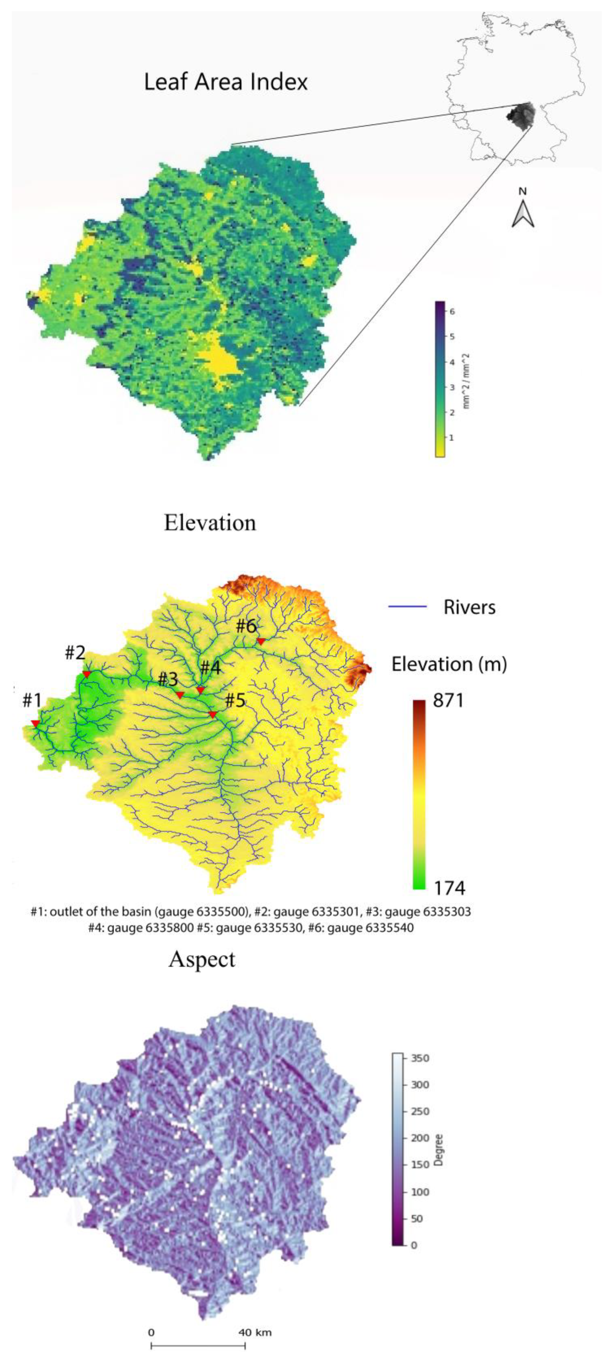
In this study, the area of the Main basin is 14,117 km². The discharge value was taken from the outlet, which is in Würzburg. Annual discharge 243 mm. The annual precipitation is 736 mm, and the potential evapotranspiration is 773 mm. Snowmelt in the spring months causes high discharge values. The discharge increases between January and April and decreases between September and November. The reason for selecting the Main Basin is that the gauge station has long-term discharge data without missing values. The location of the Main Basin in Germany, leaf area index (LAI) in summer, elevation and gauge position in the basin, river network, and aspect driven from digital elevation model (DEM) of the Main Basin are shown in Figure 1.

2.2. AET (Actual Evapotranspiration)

Actual evapotranspiration is the second important process of water balance after precipitation. About sixty percent of precipitation on land is transpired back into the air via evaporation and transpiration. Evaporated water comes from the soil, the surface of the water, and canopy interception; transpiration comes from plant leaves. Despite the leaf area index, the vegetation type is also an effective factor in AET. The driving variable of AET could be different for each basin [19].

Photosynthesis is an important process of transpiration, and the photosynthesis rate changes with the illumination angle on leaves [20]. Therefore, the aspect ratio affects transpiration and AET with leaf area index.

In mountainous basins, it is logical to use the aspect ratio for AET correction, but the basin, which has a low elevation difference, is found to be unpractical. By downscaling the referenced ET, the user may use the dynamic scaling algorithm that was proposed here to overlay the pattern of LAI on the simulated AET patterns. The idea of a crop coefficient, which is used to transform reference ET into a potential amount of evapotranspiration (PET) for a specific vegetation that is different from the reference crop, like the idea of a dynamic scaling function (DSF) introduced by Demirel et al. [8]. DSF of LAI is shown equation at the below.

$$\mathrm{DSF} =\mathrm{a}+\mathrm{b}\left(1-{\mathrm{e}}^{-\mathrm{c} \mathrm{LAI}}\right)$$

(1)

$${\mathrm{PET}=\mathrm{DSF}\ast \mathrm{ET}}_{ref}$$

(2)

“a” is the intercept term that symbolizes uniform scaling, “b” is the parameter that symbolizes vegetation dependence, and “c” identifies the rate of nonlinearity of LAI dependence [8].

2.3. mHM (Mesoscale Hydrological Model)

The mesoscale Hydrological Model (mHM) was developed by UFZ (Helmholtz Centre for Environmental Research) [21,22]. mHM is a fully distributed, physically based, and continuous model. The feature that distinguishes mHM from other hydrological models is that it is distributed with cells (grids). There are many different parameters used for each cell in the workspace. It has been successfully used in many previous studies focusing on spatial model calibration and sensitivity analysis [7,8,23,24,25].

As the resolution of the basin increases, the variability of the basin characteristics in the computer environment can be well represented. Spatial variables of inputs and state variables were analyzed on their resolution in three different layers at different scales: Level 0 (morphology), Level 1 (hydrology), and Level 2 (meteorology) (see Figure 2).

Level 0 is the highest resolution level. At this level, ground characteristics, morphological variables, land cover, and vegetation are processed. Spatial resolution processing is performed up to about a hundred meters at Level 0 is done. Level 1 is the level where hydrological processes are performed at spatial resolutions between one km–sixteen km. Finally, in Level 2, meteorological inputs and variables are processed. The resolution of Level 2 is between one km and twenty-five km. Examination of the basins based on cells can reflect the heterogeneous nature of the land. Ordinary differential equations (ODE) were used to overcome the continuity problem, which is an examination of basin based on cells. Each cell with ODEs simulates the following processes: soil moisture dynamics, snow accumulation and melting, canopy interception, infiltration and surface runoff, evapotranspiration, subsurface storage and discharge generation, deep percolation and baseflow, and discharge attenuation and flood routing [22].

The execution of output-generating hydrological model routines occurs at a scale between high-resolution watershed features and low-resolution meteorological forcing. Model parameters are regionalized by simple and built-in transfer functions that relate spatially scattered watershed properties to continuous parameter fields. With just a few calibration parameters, efficient model calibration is possible because of the control of transfer functions by global parameters. Additionally, it has been established that the mHM parameters are scale-independent, making it possible to calibrate the model at low spatial resolution and subsequently apply it at high spatial resolution using the same parameters. mHM has two transfer functions to increase the output of the geographically distributed model’s realism even further. To consider diverse land cover, it first couples completely dispersed vegetation features, namely the remotely sensed LAI, to a spatially distributed crop coefficient. Second, it derives a field capacity based on a regionally variable root depth parameter using spatially distributed information on soil texture. For a spatial model-oriented calibration framework that seeks to improve the realism of spatially distributed model simulations, both transfer functions are crucial for the efficient integration of satellite-based measurements [26]. To simulate AET, the mHM considers processes such as canopy interception, infiltration, surface runoff, base flow, deep percolation, flood routing, groundwater storage, snow-ice melting, and accumulation. Soil texture, digital elevation model, and land cover are physiographical data that are used to build the model. Land cover data were classified into three classes such as forest, pervious, and impervious cover [27]. For the simulation of actual evapotranspiration, several methods are available in mHM, such as Penman–Monteith [28], Priestley–Taylor [29], and Hargreaves–Sammani methods. The model also uses direct PET input calculated outside the model, and it can be scaled with aspect-driven and LAI-driven methods [7,30]. Previous research comparing LAI or aspect can be found in the literature [7,8,9].

As a result of the ODEs analyzed for these processes, the hydrograph for each cell is obtained. The resulting hydrographs are between cells in Level 1. The Muskingum method is used between cells, and flow routing is obtained with this translation until the outlet. Unlike lumped models, altitude information from DEM, flow direction and flow accumulation maps are all used to route the runoff from one cell to other [4].

2.4. Meteorologic, Morphologic, and Hydrologic Data

Meteorological data was taken from E-OBS (European observation) and MODIS (moderate resolution imaging spectroradiometer), morphology from SRTM (shuttle radar topography mission), ESD (European soil database), and HWSD (harmonized world soil database), hydrology from GRDC (global runoff data center). E-OBS is a daily gridded dataset that observes daily precipitation, daily mean temperature, daily maximum temperature, and daily minimum temperature. Temperature and precipitation were taken from E-OBS. Files are provided in netCDF-4 format, and the cover area is between 25° N–71.5° N × 25° W–45° E [31]. Leaf area index (LAI) and land cover data were received from the MODIS dataset. The best image is selected by algorithm from sensors that are placed on NASA’s Terra and Aqua satellites within eight-day periods [32,33]. DEM (digital elevation model) was received from SRTM (The Shuttle Radar Topography Mission). SRTM compares slightly different angles comes from two radar signals to calculate surface elevation. SRTM covers eighty percent of Earth between 60° N–56° S [34]. Soil classes received from ESDB. ESDB is s basic representation of soil classes on the spatial pattern in Europe. The ESDB has seventy-three features of soil classes such as parent material, impermeable layer, restriction on agricultural use, soil water regime, altitude, slope, and physical, chemical, mechanical, and hydrological characteristics [35]. Soil class information is also obtained from HWSD. HWSD is a worldwide combination of soil maps and has more than sixteen thousand soil attribute units. The raster map of HWSD has 21,600 rows and 43,200 columns, which have characterization such as organic carbon, pH, soil depth, total exchangeable nutrients, gypsum and lime concentration, sodium exchange percentage, salinity, textural class, and granulometry [36]. Daily discharge values of six gauges (#6335500, #6335301, #6335303, #6335800, #6335530, and #6335540) were received from GRDC. All inputs are summarized in

Table 1. Description of morphologic and meteorologic inputs of mHM and their resolution and dataset resources [31,34,36,37,38,39].

Variable	Description	Resolution Degree	Source
Q (daily)	Streamflow	Point	GRDC
P (daily)	Precipitation	0.0625	EOBS
AETref (daily)	Actual evapotranspiration	0.0625	MODIS
PETref (daily)	Potential evapotranspiration	0.0625	E-OBS
Tavg (daily)	Average air temperature	0.0625	E-OBS
LAI	Fully distributed monthly values based on an 8-day time-varying Leaf Area Index (LAI) dataset	0.001953125	MODIS
Land cover	Forest, pervious and urban	0.001953125	MODIS
DEM related data	Slope, aspect, flow accumulation, and direction	0.001953125	SRTM
Geology class	Two main geological formations	0.001953125	UFZ-Leipzig
Soil class	Fully distributed soil texture data	0.001953125	HWSD and ESD

GRDC: https://www.bafg.de/GRDC/EN/Home/homepage_node.html; (accessed on 2 April 2014). E-OBS: https://www.ecad.eu/download/ensembles/ensembles.php; (accessed on 2 April 2014). MODIS: https://lpdaac.usgs.gov/tools/usgs-earthexplorer/; (accessed on 2 April 2014). SRTM: https://www.usgs.gov/centers/eros/science/usgs-eros-archive-digital-elevation-shuttle-radar-topography-mission-srtm; (accessed on 2 April 2013). HWSD: http://webarchive.iiasa.ac.at/Research/LUC/External-World-soil-database/HTML/; (accessed on 2 April 2014). ESD: https://publications.jrc.ec.europa.eu/repository/handle/JRC83425; (accessed on 2 April 2014). UFZ: https://www.ufz.de/index.php?en=40113; (accessed on 2 April 2014).

.

2.5. Leaf Area Index (LAI) and Actual Evapotranspiration (AET)

MODIS, which is a global ET algorithm in NASA’s Earth Observation System, was developed for hydrological and ecological research using remote sensing data. During the calibration process of this study, ET data was obtained from the MOD15 algorithm at eight-day, monthly, and yearly intervals with one-kilometer spatial resolution. MODIS LAI product as a long-term monthly average was inserted into the model. LAI maps of plant growth on low-resolution PET data are used to introduce the dynamics of PET and directly affect the results of the AET [7]. Leaf Area Index (LAI) is taken into consideration at the L0 level and upscaled from L0 to the L1, and LAI is calculated as in the equation below [40]:

$$\mathrm{Leaf} \mathrm{Area} \mathrm{Index}= \mathrm{Leaf} \mathrm{area} \mathrm{per} \mathrm{plant} \times \mathrm{Number} \mathrm{of} \mathrm{plants} \mathrm{per} \mathrm{unit} \mathrm{area}$$

(3)

2.6. Aspect and Actual Evapotransporation (AET)

Aspect, which is a Digital Elevation Model (DEM) related data, is a very effective parameter for snow cover [41]. It was taken the consideration with LAI to obtain a more accurate prediction of evapotranspiration on both mountain and low-elevation variety basins.

The original scaling factor in mHM is based on an aspect-driven term and a lumped minimum correction. In mountainous areas, considering the aspect ratio for AET correction is very logical, but this is found to be irrelevant for a basin which has a low elevation difference [8].

2.7. Objective Functions

2.7.1. Kling-Gupta Efficiency (KGE)

KGE takes values equal or smaller than ideal point one.

$$\mathrm{KGE}=1-\mathrm{ED}$$

(4)

$$\mathrm{ED}=\sqrt{{\left(\mathsf{\alpha }-1\right)}^2+{\left(\mathsf{\beta }-1\right)}^2+{\left(\mathsf{ɣ}-1\right)}^2}$$

(5)

“$\mathsf{\alpha }$” is the Pearson correlation coefficient. “$\mathsf{\beta }$” is the ratio between the average of the forecast values and the average of the observed values. “$\mathsf{ɣ}$” is the ratio between the standard deviation of forecast values and the standard deviation of observation, and “ED” is Euclidian distance from the ideal point zero [42]. The objective function is revised as 1-KGE since the optimizers search for the minimum point i.e., zero in this case.

2.7.2. Spatial Efficiency Metric (SPAEF)

In this case, aspect-driven results have been checked. SPAEF metric consists of correlation, coefficient of variation, and histogram match. These components help to overcome sophisticated hydraulic models [25].

$$\mathrm{SPAEF}=1-\sqrt{{\left(\mathsf{\alpha }-1\right)}^2+{\left(\mathsf{\beta }-1\right)}^2+{\left(\mathsf{ɣ}-1\right)}^2}$$

(6)

$$\mathsf{\alpha }=\mathsf{\rho }(\mathrm{obs},\mathrm{sim}), \mathsf{\beta }=(\frac{{\sigma }_s}{{\mu }_s})/(\frac{{\sigma }_o}{{\mu }_o}), \mathsf{ɣ}=\frac{{{\displaystyle \sum }}_{j=1}^n\min \left(K_j,L_j\right)}{{{\displaystyle \sum }}_{j=1}^n{K}_j}$$

(7)

“α” is the Pearson correlation coefficient which shows the correlation between observed and simulated values. “β” symbolizes spatial variability, which is the fraction of the coefficient of variation. “$\mathsf{ɣ}$” stands for histogram intersection, K refers to observed pattern, and L refers to simulated pattern.

2.8. Model Calibration and Validation

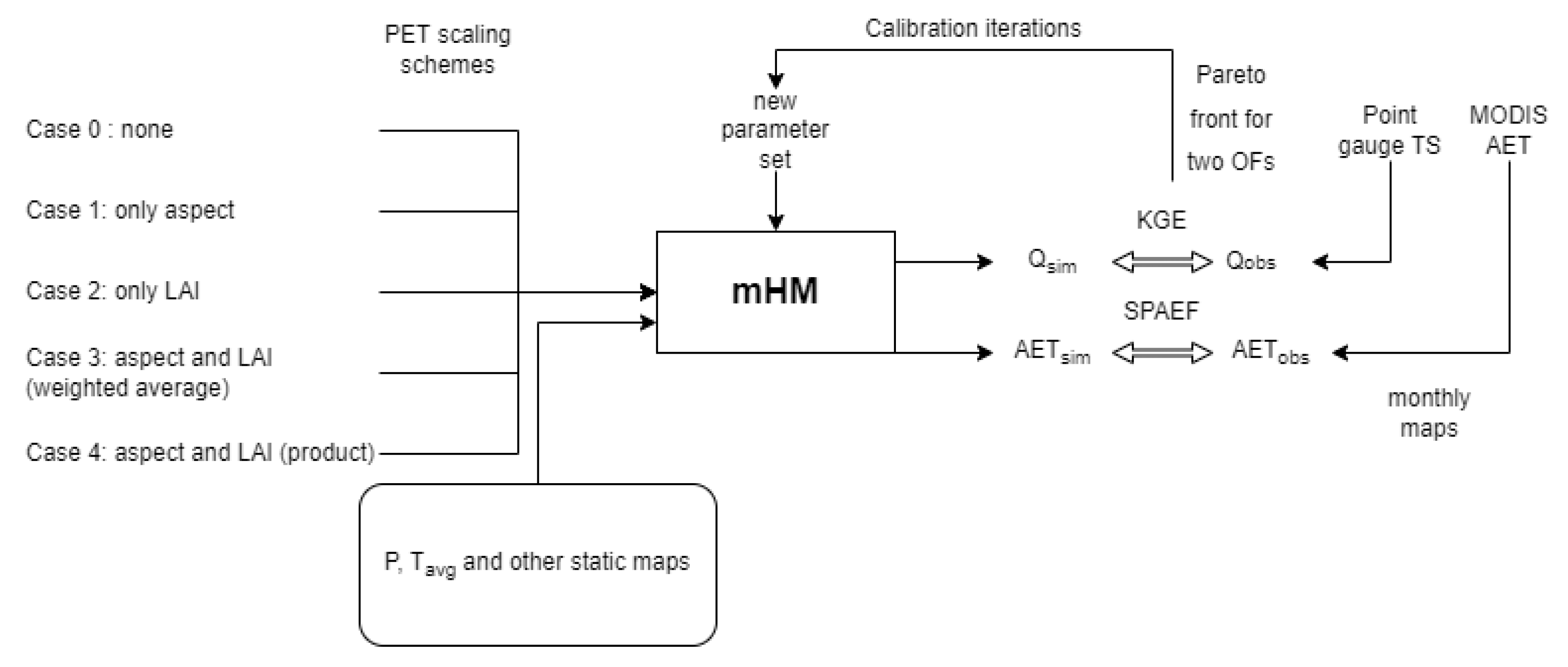
For five different cases, sensitive parameters are calibrated with seven hundred fifty iterations by OSTRICH (Optimization Software Toolkit). There is more than one objective function. Therefore, the PADDS (Pareto Archived Dynamically Dimensioned Search) algorithm is preferred. Pareto-front select non-dominated runs in seven hundred fifty runs. Non-dominated runs provide a choice to the user between objective functions to select a parameter set and group for the next model application. Non-dominated runs maintain improvement on both objective functions simultaneously. The PADDS produces components randomly in the distribution of runs along the Pareto front. The tradeoff between the spatial ET performance and the temporal discharge performance is clearly shown in all cases as a Pareto front. The SPAEF residuals after normalization were more different from the normalized target pattern than the original ET patterns. However, water balance performance is comparable between cases [26]. The calibration scheme for four cases is shown in Figure 3.

OSTRICH minimizes the objective function of KGE and SPAEF. The ideal value for KGE and SPAEF is one. The square residual defined for SPAEF for the spatial pattern of AET is (8), and the sum of the six-gauge square residual defined for KGE is (9).

$$S{R}_{AET}= {\left(1-SPAEF\right)}^2$$

(8)

$$SS{R}_Q={{\displaystyle \sum }}_i^6{\left(1-KG{E}_i\right)}^2$$

(9)

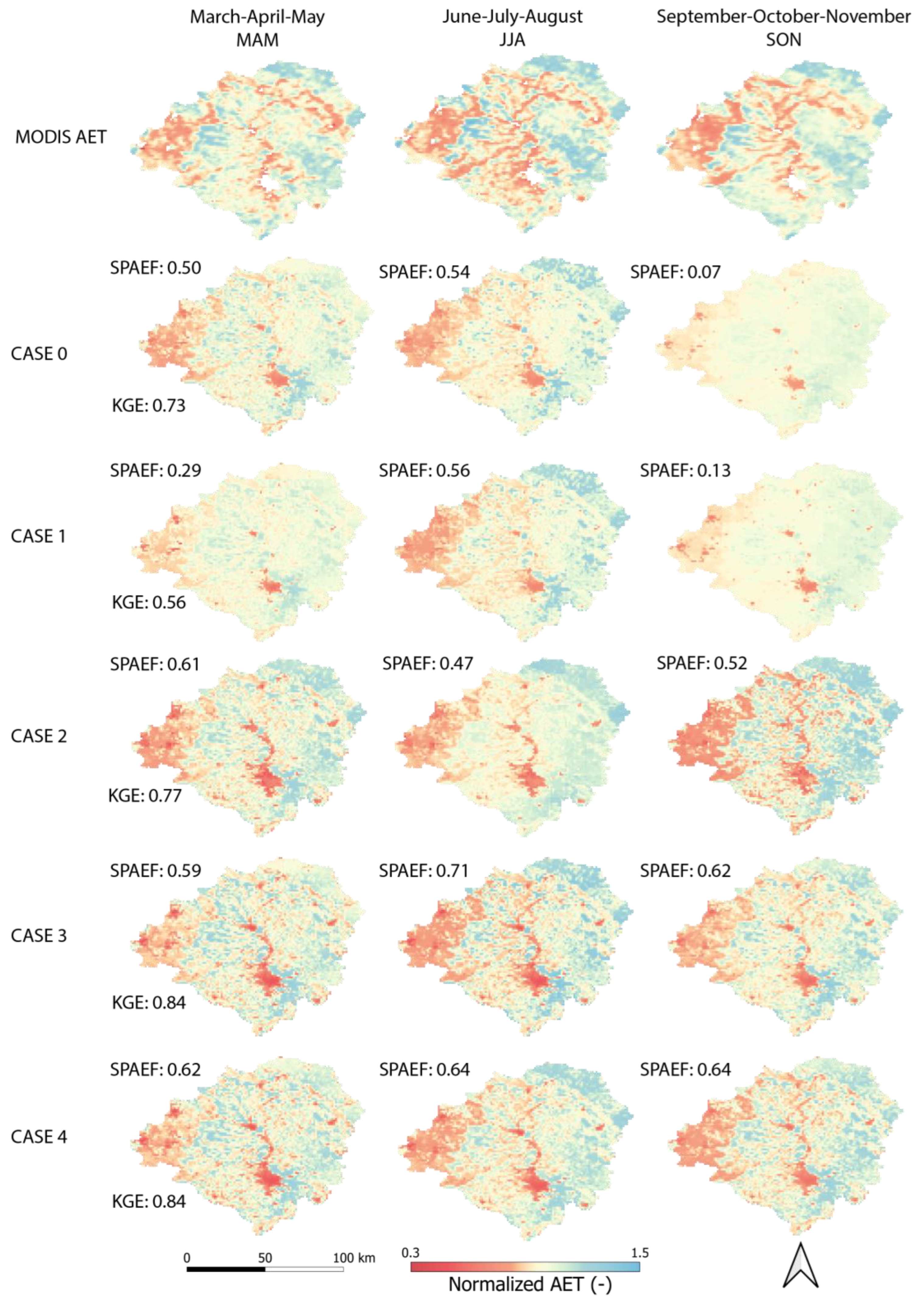
MODIS AET values are monthly maps between 2002 and 2014. AET maps were compared with simulated seasons which are March–April–May (MAM), June–July–August (JJA), and September–October–November (SON). At the end of the iteration, the best parameter sets were selected for every case, and they ran once more to validate the results. The best parameter sets were selected as the smallest value of the sum of the objective function of KGE and the objective function of SPAEF.

Case 0, PET correction was driven by neither LAI nor aspect. The purpose of adding this case is to see the vegetation and aspect effect by comparing other cases. Case 1, aspect-driven results were checked. Aspect, whose unit is degree, is the compass direction of hillslope faces. Case 2, LAI-driven results were checked. LAI, which is a unitless parameter, is the ratio of the vegetation area to the total area.

Case 3, the LAI and aspect driven by the weight number (alphax) results were checked. LAI and aspect were driven by the weight parameter between zero and one. LAI multiplied by alphax, and aspect was multiplied by (1-alphax) and summed for AET correction. PET correction method was added mHM source file like in Equation (10) [43].

$$pet=pet\_in\left(k\right)\times \left(\left(petLAIcorFactorL1\left(k\right)\times alphax\right)+\left(fAsp\left(k\right)\times \left(1-alphax\right)\right)\right)$$

(10)

Case 4, the LAI and aspect correction numbers were multiplied for PET correction, and the results were checked. This case added to search the effect of aspect on photosynthesis and the effect of both on actual evapotranspiration. Equation (11) was added to the methods of mHM [43].

$$pet=pet\_in\left(k\right)\times petLAIcorFactorL1\left(k\right)\times fAsp\left(k\right)$$

(11)

3. Results

3.1. Model Sensitivity Analysis

Hydrological modeling is necessary for scenario analysis in agronomy to manage crops and water resources effectively. The functions of a natural system are often represented by highly parameterized, physically justified, process-based numerical models. This allows the models to be used to assess the effectiveness of management strategies or the system’s response to environmental changes [44].

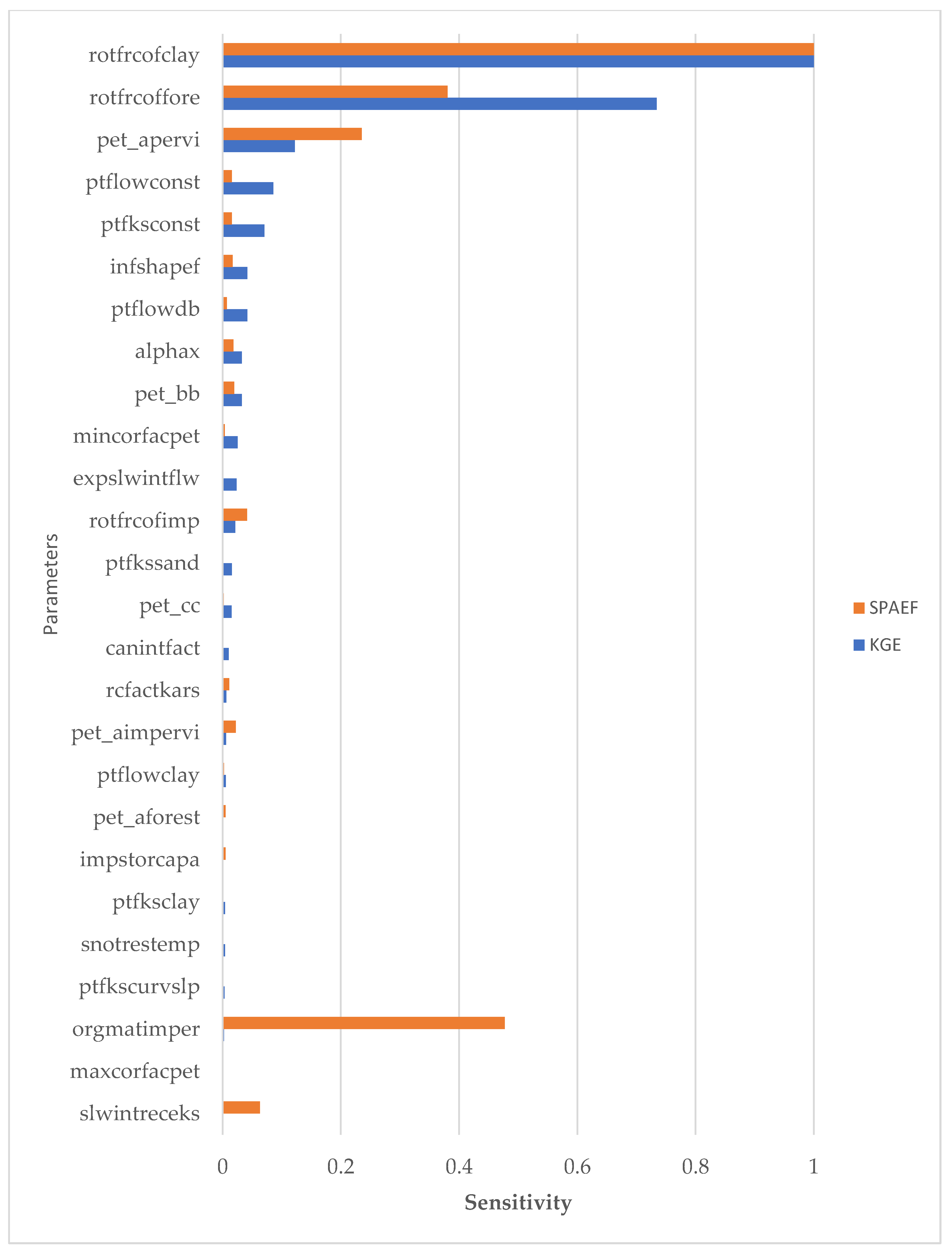
All morphological and meteorological data transform to appropriate resolution and time scale. Instead of using all sixty-nine parameters of mHM, the most sensitive twenty-six parameters were used for this study. Considering all parameters causes time consumption; therefore, sensitivity analysis based on objective functions was calculated with Model-Independent Parameter Estimation and Uncertainty Analysis (PEST) [44] by the objective function of SPAEF and KGE metrics. Objective functions are SPAEF for the spatial pattern of actual evapotranspiration and KGE for six discharge gauges.

The most sensitive twenty-six parameters are shown in Figure 4. These parameters were selected based on the combined sensitivity of KGE and SPAEF. Based on KGE, the most sensitive 10 parameters controlling water balance include soil, LAI, aspect parameters, and alphax. The other objective function of SPAEF is also sensitive to similar parameters. PET parameters also affect KGE. Soil properties showed a significant impact on SPAEF.

All sensitive parameters were normalized between zero and one. The description and the range of parameters are shown in

Table 2. Description of twenty-six selected sensitive parameters and their ranges in mHM.

Parameter Name	Description	Min	Max
rotfrcofclay	root fraction coefficient clay	0.9	0.999
rotfrcoffore	root fraction coefficient forest	0.9	0.999
pet_apervi	PET scaling: pervious	−0.3	1.3
ptflowconst	PTF saturated water content: constant	0.6462	0.9506
ptfksconst	PTF hydraulic conductivity: constant	−1.5	−1.2
infshapef	Infiltration shape factor	1	4
ptflowdb	PTF saturated water content: coefficient bulk density	−0.3727	−0.1871
alphax	Weight parameter between LAI and aspect	0	1
pet_bb	PET scaling: range	0	1.5
mincorfacpet	minimum correction factor of PET	0.7	1.3
orgmatimper	Organic matter content for impervious zone	0	1
rotfrcofimp	Root fraction coefficient impervious	0.9	0.999
ptfkssand	PTF hydraulic conductivity: Sand	0.0042	0.01
pet_cc	PET scaling: shape	−2	0
canintfact	Canopy interception factor	0.15	0.4
rcfactkars	Recharge factor karstic	−5	5
pet_aimpervi	PET scaling: impervious	0.3	1.3
ptflowclay	PTF saturated water content: clay	0.0001	0.0029
ptfksclay	PTF hydraulic conductivity: clay	0.003	0.0129
snotrestemp	Snow temperature threshold for rain and snow separation	−2	2
ptfkscurvslp	PTF hydraulic conductivity: curve slope	51	56
slwintreceks	Slow interception	1	30
impstorcapa	Impervious storage capacity	0	5
pet_aforest	PET scaling: forest	0.3	1.3
aspectreshpet	Aspect threshold PET	160	200
maxcorfacpet	Maximum correction factor of PET	0	0.2

. As shown in Figure 4 weight parameter between LAI and aspect (alphax) is the eighth most sensitive parameter not only for KGE for gauges but also for SPAEF for actual evapotranspiration.

3.2. Spatial Pattern Result of AET

In Germany, the Main Basin is modeled by a fully distributed hydrologic model mHM. For two objective functions (KGE and SPAEF), the best-balanced solution was chosen for visualization. SPAEF value for AET and KGE value for outlet discharge were calculated within a three-month period for evaluated cases. Three-month periods are MAM (March, April, and May), JJA (June, July, and August), and SON (September, October, and November).

The results are according to the best case in non-dominated solutions. If there is no other better solution in two objective functions is called non-dominated. All cases were compared with MODIS AET data in Figure 5. The best non-dominated solution (minimum summation of KGE and SPAEF) nearest to the origin selected to visualize.

According to the result of spatial pattern, ignoring aspect and LAI for AET in Case 0 causes the worst result in three terms (SPAEFs are 0.50, 0.54, and 0.07). KGE is 0.73. KGE of base case performs better than Case 1. Spatial pattern performances are also not too bad based on JJA and MAM because there are more sensitive parameters than LAI and aspects such as soil and land cover. Therefore, results were not irrelevant to observed MODIS AET, even though it was driven by neither LAI nor aspect.

According to the result of Case 1 (aspect-driven), the aspect correction improved the AET performance. Three-term SPAEF results are 0.29, 0.56, and 0.13). KGE result is 0.56. Case 1 spatial pattern results were slightly better than Case 0. In snow-dominated mountainous basins, aspect-driven case may reveal better results than these results.

The result of Case 2 (LAI driven) showed much better performance than Case 0 and Case 1. LAI effect was more significant than the aspect in the Main Basin. Three-term SPAEF results are 0.61, 0.47, and 0.52. KGE result is 0.77. Case 2 result is much better than Case 0 and Case 1. This result is very similar to previous studies [7,8].

The weight parameter between LAI and aspect is a number between zero and one. LAI was multiplied by the weight parameter, and the aspect was multiplied by (1-weight parameter) and summed for AET correction. Case 3 performance was better than other cases. Three-term SPAEF results were 0.59, 0.71, and 0.62. KGE result is 0.84, which was much better than other cases. The weight parameter helped better constrain the model parameters connected to actual evapotranspiration when compared to cases based on only LAI or aspect.

Case 4 also shows good results like Case 3. SPAEF values for the spatial pattern of AET are 0.62, 0.62, and 0.64. KGE is 0.64. The LAI-driven correction parameter was multiplied with aspect and PET. The “alphax “parameter was not used in this case. This shows that without adding new parameters, just influencing LAI and aspect to model enough to get a much better result. Case 3 and Case 4 spatial pattern and water balance performance were very close.

3.3. Water Balance Result of Gauges

Simulated KGE results according to observed discharges are shown in

Table 3. Model validation gauges from internal tributaries of the Main Basin.

	KGE
Gauges	CASE 0	CASE 1	CASE 2	CASE 3	CASE 4
6335500	0.14	0.3	0.07	0.55	0.30
6335301	0.13	0.28	0.04	0.54	0.28
6335303	−0.03	0.21	−0.24	0.48	0.07
6335530	−0.67	−0.03	−0.85	−0.01	−0.46
6335800	0.57	0.53	0.45	0.67	0.52
6335540	−4.38	−3.49	−4.62	−4.07	−4.94

Validations were also run also with six gauges. Case 3 and Case 4 show better KGE performance in most of the gauges. The location of the gauges is shown in Figure 1 Based on these gauges, the KGE discharge result compared to observed data is shown in Table 3. Improved performance of Case 3 and Case 4 was observed in most of the gauges. The most surprising aspect of the data was that the water balance score of Case 3 was better than Case 4. Instead of single outlet gauge validation, Case 3 is more compatible with multigauge calibration than Case 4.

3.4. Non-Dominated Result and Best Parameter of Cases

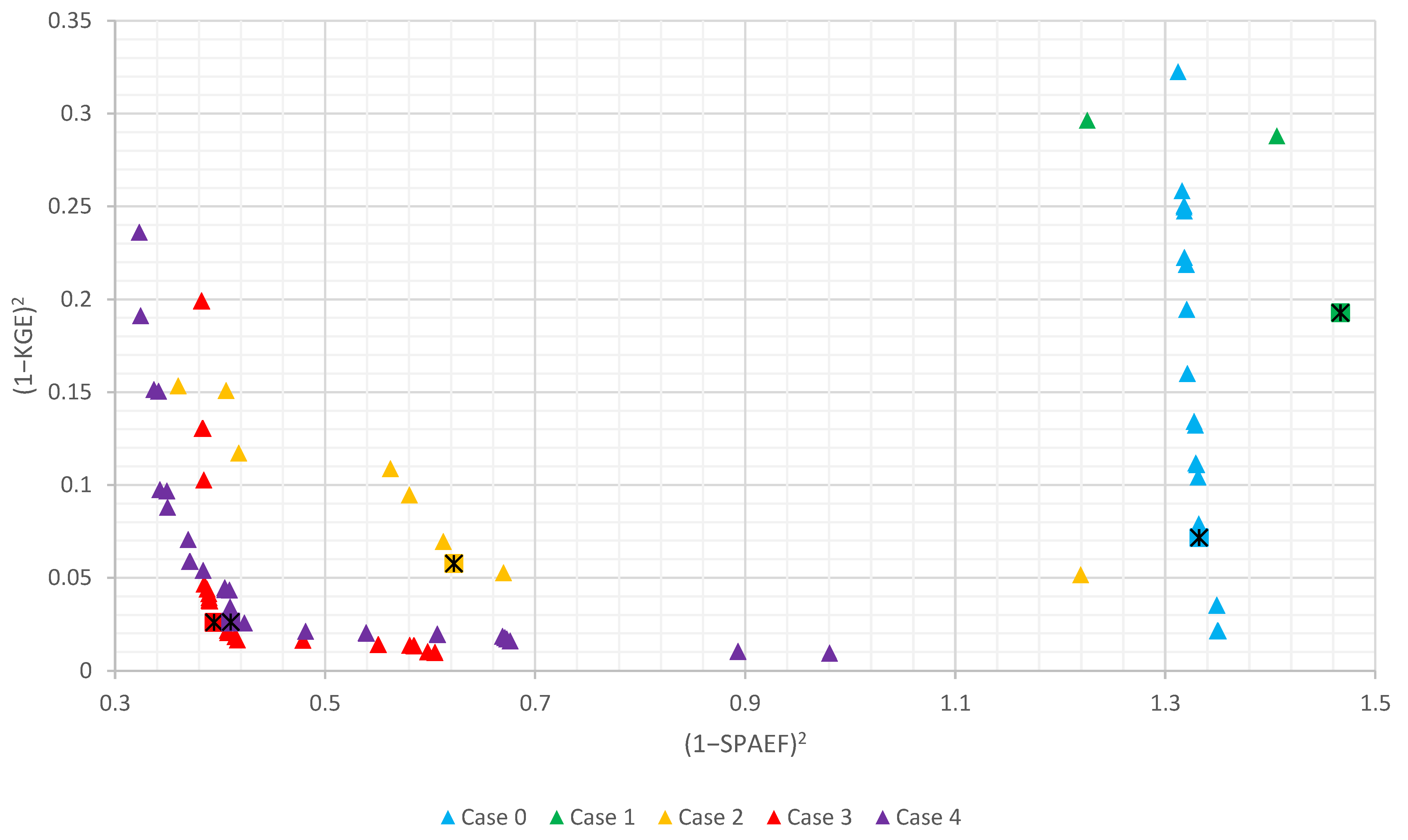
After seven hundred fifty iterations, selected non-dominated solutions and marked best cases are represented in Figure 6.

Theo objective functions of KGE and SPAEF are shown in the axis. The closest point of each case was marked as the best parameter set of those cases. Case 0 (blue) and Case 1 (green) have extremely poor SPAEF performance and poor KGE performance, as expected. Increased performance with LAI is also clearly visible in Case 2 (yellow). Case 3 and Case 4 performance are better than all other cases. The best result of Case 3 is slightly better than that of Case 4. However, the spatial pattern score of Case 4 is better in many calculations. On the contrary, the streamflow score of Case 3 was better in some of the calculations. Taken together, these results suggest that there is an association between LAI and the aspect to calibrate the hydrologic model.

4. Discussion

The present study was designed to determine the effect of LAI and the aspect on hydrologic models. For this purpose, four cases were designed from Case 0 to Case 4 with different inputs and varying equations. Case 0 was configured without LAI and aspect correction. Case 1 was designed with aspect and Case 2 with LAI only. In Case 3, the coefficient was added to LAI and aspect correction and summed. Case 4 was built by multiplying LAI and aspect correction, which makes it possible to observe model performance without adding a parameter.

The most obvious finding to emerge from the analysis was that simulation performed better results when LAI and aspect were used together. The spatial pattern of AET of Case 2 is much more similar than the spatial pattern of Case 0 and Case 1. This result seems to be consistent with other research [7,9]. Snow-dominated, rain-dominated, or basins that have different types of vegetation may differ in rate of effect between aspect and LAI. However, in any case, both LAI and aspect effect is important. Aspect-related studies [16,17] show facing slope effect on vegetation and AET. Much uncertainty still exists about the effect of both LAI and aspect on AET. According to sixty different catchment studies, aspect-driven sites show different crop types between (polar-facing slopes) PFS and (equatorial-facing slopes) EFS [16]. Therefore, beyond the effect of LAI and aspect on AET, aspect influences LAI. Case 3 and Case 4 should also be tested in different types of basins. For example, mountainous areas, snow-dominated areas, or in basins with different climates.

5. Conclusions

The main goal of this study is to assess the effect of LAI and aspect together on the model simulated AET and water balance. For this purpose, five cases (experiments) are designed for the Main Basin (Germany) with a fully distributed hydrologic model mHM. Firstly, the source code of mHM is modified and added a new parameter, i.e., alphax. Then, sensitive parameters are determined for calibration. For each case, discharge was calibrated with KGE metric by comparing with measured outlet discharge, and the spatial pattern of AET was calibrated with the objective function of SPAEF by comparing with MODIS AET monthly data. The following conclusions are drawn based on the calibration and validation results:

• Using unscaled PET is sufficient for a reasonable water balance like in lumped models.
• Using only the aspect for PET scaling deteriorates water balance performance and not improves the AET performance.
• Using only monthly LAI maps for dynamic PET scaling significantly improves the AET and water balance performance of the mHM.
• The product of LAI and aspect without weighting also improves the AET and water balance performance of mHM.
• The weighting LAI and aspect using alphax parameter reveals slightly better performance than the product of LAI and aspect.

Further research will explore the added value of daily LAI maps instead of monthly maps on dynamic PET correction.

References

- Zhang, X.; Srinivasan, R.; Zhao, K.; Liew, M. Van Evaluation of global optimization algorithms for parameter calibration of a computationally intensive hydrologic model. Hydrol. Process. 2009, 23, 430–441. [Google Scholar] [CrossRef]
- Li, J.; Chen, H.; Xu, C.-Y.; Li, L.; Zhao, H.; Huo, R.; Chen, J. Joint Effects of the DEM Resolution and the Computational Cell Size on the Routing Methods in Hydrological Modelling. Water 2022, 14, 797. [Google Scholar] [CrossRef]
- Gong, L.; Widén-Nilsson, E.; Halldin, S.; Xu, C.-Y. Large-scale runoff routing with an aggregated network-response function. J. Hydrol. 2009, 368, 237–250. [Google Scholar] [CrossRef]
- Alp, H.; Demirel, M.C. Hydrological Model Structure and Calibration Algorithm Effect on Discharge Simulation Performance. In Proceedings of the International Graduate Research Symposium IGRS’22, Istanbul, Turkey, 1–3 June 2022; ITU-LEE: İstanbul, Turkey, 2022. [Google Scholar]
- Alp, H.; Demirel, M.C.; Aşıkoğlu, Ö.L. Effect of Model Structure and Calibration Algorithm on Discharge Simulation in the Acısu Basin, Turkey. Climate 2022, 10, 196. [Google Scholar] [CrossRef]
- Zhao, L.; Xia, J.; Xu, C.; Wang, Z.; Sobkowiak, L.; Long, C. Evapotranspiration estimation methods in hydrological models. J. Geogr. Sci. 2013, 23, 359–369. [Google Scholar] [CrossRef]
- Avcuoglu, M.B.; Demirel, M.C. On the Utility of Remotely Sensed Actual ET and LAI in Hydrologic Model Calibration. Tek. Dergi 2022, 33, 13020. [Google Scholar] [CrossRef]
- Demirel, M.C.; Mai, J.; Mendiguren, G.; Koch, J.; Samaniego, L.; Stisen, S. Combining satellite data and appropriate objective functions for improved spatial pattern performance of a distributed hydrologic model. Hydrol. Earth Syst. Sci. 2018, 22, 1299–1315. [Google Scholar] [CrossRef]
- Busari, I.O.; Demirel, M.C.; Newton, A. Effect of Using Multi-Year Land Use Land Cover and Monthly LAI Inputs on the Calibration of a Distributed Hydrologic Model. Water 2021, 13, 1538. [Google Scholar] [CrossRef]
- Wang, Q.J. The Genetic Algorithm and Its Application to Calibrating Conceptual Rainfall-Runoff Models. Water Resour. Res. 1991, 27, 2467–2471. [Google Scholar] [CrossRef]
- Dawdy, D.R.; O’Donnell, T. Mathematical Models of Catchment Behavior. J. Hydraul. Div. 1965, 91, 123–137. [Google Scholar] [CrossRef]
- Kuczera, G. On the validity of first-order prediction limits for conceptual hydrologic models. J. Hydrol. 1988, 103, 229–247. [Google Scholar] [CrossRef]
- Gupta, H.V.; Sorooshian, S.; Yapo, P.O. Toward improved calibration of hydrologic models: Multiple and noncommensurable measures of information. Water Resour. Res. 1998, 34, 751–763. [Google Scholar] [CrossRef]
- Harlin, J. Development of a Process Oriented Calibration Scheme for the HBV Hydrological Model. Hydrol. Res. 1991, 22, 15–36. [Google Scholar] [CrossRef]
- Shamir, E.; Imam, B.; Gupta, H.V.; Sorooshian, S. Application of temporal streamflow descriptors in hydrologic model parameter estimation. Water Resour. Res. 2005, 41, 1. [Google Scholar] [CrossRef]
- Kumari, N.; Saco, P.M.; Rodriguez, J.F.; Johnstone, S.A.; Srivastava, A.; Chun, K.P.; Yetemen, O. The Grass Is Not Always Greener on the Other Side: Seasonal Reversal of Vegetation Greenness in Aspect-Driven Semiarid Ecosystems. Geophys. Res. Lett. 2020, 47, 7. [Google Scholar] [CrossRef]
- Srivastava, A.; Kumari, N.; Yetemen, O. Aspect-controlled spatial and temporal soil moisture patterns across three different latitudes. In Proceedings of the MODSIM2019, 23rd International Congress on Modelling and Simulation, Canberra, Australia, 1–6 December 2019; Modelling and Simulation Society of Australia and New Zealand: Sydney, NSW, Australia, 2019. [Google Scholar]
- Tikkanen, A. Main River. 2022. Available online: https//www.britannica.com/place/Main-River (accessed on 10 October 2022).
- Jung, I.W.; Chang, H.; Risley, J. Effects of runoff sensitivity and catchment characteristics on regional actual evapotranspiration trends in the conterminous US. Environ. Res. Lett. 2013, 8, 044002. [Google Scholar] [CrossRef]
- Paradiso, R.; de Visser, P.H.B.; Arena, C.; Marcelis, L.F.M. Light response of photosynthesis and stomatal conductance of rose leaves in the canopy profile: The effect of lighting on the adaxial and the abaxial sides. Funct. Plant Biol. 2020, 47, 639. [Google Scholar] [CrossRef] [PubMed]
- Kumar, R.; Samaniego, L.; Attinger, S. The effects of spatial discretization and model parameterization on the prediction of extreme runoff characteristics. J. Hydrol. 2010, 392, 54–69. [Google Scholar] [CrossRef]
- Samaniego, L.; Kumar, R.; Attinger, S. Multiscale parameter regionalization of a grid-based hydrologic model at the mesoscale. Water Resour. Res. 2010, 46, W05523. [Google Scholar] [CrossRef]
- Demirel, M.C.; Özen, A.; Orta, S.; Toker, E.; Demir, H.K.; Ekmekcioğlu, Ö.; Tayşi, H.; Eruçar, S.; Sağ, A.B.; Sarı, Ö.; et al. Additional Value of Using Satellite-Based Soil Moisture and Two Sources of Groundwater Data for Hydrological Model Calibration. Water 2019, 11, 2083. [Google Scholar] [CrossRef] [Green Version]
- Stisen, S.; Soltani, M.; Mendiguren, G.; Langkilde, H.; Garcia, M.; Koch, J. Spatial Patterns in Actual Evapotranspiration Climatologies for Europe. Remote Sens. 2021, 13, 2410. [Google Scholar] [CrossRef]
- Koch, J.; Demirel, M.C.; Stisen, S. The SPAtial EFficiency metric (SPAEF): Multiple-component evaluation of spatial patterns for optimization of hydrological models. Geosci. Model Dev. 2018, 11, 1873–1886. [Google Scholar] [CrossRef]
- Koch, J.; Demirel, M.C.; Stisen, S. Climate Normalized Spatial Patterns of Evapotranspiration Enhance the Calibration of a Hydrological Model. Remote Sens. 2022, 14, 315. [Google Scholar] [CrossRef]
- Rakovec, O.; Kumar, R.; Mai, J.; Cuntz, M.; Thober, S.; Zink, M.; Attinger, S.; Schäfer, D.; Schrön, M.; Samaniego, L. Multiscale and Multivariate Evaluation of Water Fluxes and States over European River Basins. J. Hydrometeorol. 2016, 17, 287–307. [Google Scholar] [CrossRef]
- Monteith, J.L. Evaporation and Environment. Symp. Soc. Exp. Biol. 1965, 19, 205–234. [Google Scholar] [PubMed]
- Jensen, M.; Burman, R.; Allen, R. Evaporation, Evapotranspiration, and Irrigation Water Requirements; American Society of Civil Engineers: Reston, VA, USA, 2016; Volume 131. [Google Scholar] [CrossRef]
- Samaniego, L.; Brenner, J.; Craven, J.; Cuntz, M.; Dalmasso, G.; Demirel, M.C.; Jing, M.; Kaluza, M.; Kumar, R.; Langenberg, B.; et al. The mesoscale Hydrologic Model—mHM v5.11.1 (v5.11.0). 2021. Available online: https://mhm.pages.ufz.de/mhm/stable/md_doc__r_e_l_e_a_s_e_s.html#autotoc_md15 (accessed on 26 December 2022).
- Cornes, R.C.; van der Schrier, G.; van den Besselaar, E.J.M.; Jones, P.D. An Ensemble Version of the E-OBS Temperature and Precipitation Data Sets. J. Geophys. Res. Atmos. 2018, 123, 9391–9409. [Google Scholar] [CrossRef]
- Myneni, R.; Knyazikhin, Y.; Park, T. MCD15A2H MODIS/Terra+Aqua Leaf Area Index/FPAR 8-day L4 Global 500m SIN Grid V006 [Data Set]; NASA EOSDIS Land Processes DAAC: Sioux Falls, SD, USA, 2015.
- Running, S.; Mu, Q.; Zhao, M. MOD16A2 MODIS/Terra Net Evapotranspiration 8-Day L4 Global 500m SIN Grid V006 [Data Set]; NASA EOSDIS Land Processes DAAC: Sioux Falls, SD, USA, 2017. [CrossRef]
- NASA JPL. NASA Shuttle Radar Topography Mission Swath Image Data [Data Set]; NASA EOSDIS Land Processes DAAC: Sioux Falls, SD, USA, 2014. [CrossRef]
- Panagos, P.; Van Liedekerke, M.; Borrelli, P.; Köninger, J.; Ballabio, C.; Orgiazzi, A.; Lugato, E.; Liakos, L.; Hervas, J.; Jones, A.; et al. European Soil Data Ce35ntre 2.0: Soil data and knowledge in support of the EU policies. Eur. J. Soil Sci. 2022, 73, e13315. [Google Scholar] [CrossRef]
- Batjes, N.; Dijkshoorn, K.; van Engelen, V.; Fischer, G.; Jones, A.; Montanarella, L.; Petri, M.; Prieler, S.; Teixeira, E.; Shi, X.; et al. FAO/IIASA/ISRIC/ISS-CAS/JRC. Harmonized World Soil Database (Version 1.2); FAO: Rome, Italy; IIASA: Laxenburg, Austria, 2012. [Google Scholar]
- Running, S.; Mu, Q.; Zhao, M. MOD16A3 MODIS/Terra Net Evapotranspiration Yearly L4 Global 500 m SIN Grid V006 [Data Set]; NASA EOSDIS Land Processes DAAC: Sioux Falls, SD, USA, 2017. [CrossRef]
- The Global Runoff Data Centre GRDC Da ta. Available online: https://www.bafg.de/GRDC/EN/02_srvcs/21_tmsrs/210_prtl/prtl_node.html (accessed on 2 April 2014).
- Hiederer, R. Mapping Soil Properties for Europe—Spatial Representation of Soil Database Attributes. EUR26082EN Scientific and Technical Research series. JRC Tech. Rep. 2013, 47, 1831–9424. [Google Scholar] [CrossRef]
- Liu, Z.; Wei, S.; Li, M.; Zhang, Q.; Zong, R.; Li, Q. Response of Water Radiation Utilization of Summer Maize to Planting Density and Genotypes in the North China Plain. Agronomy 2022, 13, 68. [Google Scholar] [CrossRef]
- Doumit, J.; Sakr, S. Toward a snow melt prediction map of Mount Lebanon. InterCarto InterGIS 2019, 25, 16–27. [Google Scholar] [CrossRef]
- Gupta, H.V.; Kling, H.; Yilmaz, K.K.; Martinez, G.F. Decomposition of the mean squared error and NSE performance criteria: Implications for improving hydrological modelling. J. Hydrol. 2009, 377, 80–91. [Google Scholar] [CrossRef]
- Demirci, U.; Demirel, M.C. PET scaling method with LAI and aspect in mHM. Zenodo 2022. [Google Scholar] [CrossRef]
- White, J.T.; Hunt, R.J.; Fienen, M.N.; Doherty, J.E. Approaches to highly parameterized inversion: PEST++ Version 5, a software suite for parameter estimation, uncertainty analysis, management optimization and sensitivity analysis. Tech. Methods 2020, 64. [Google Scholar] [CrossRef]
Figure 1.
Physical characteristics (LAI, DEM, and aspect maps) of the study domain, i.e., the Main Basin in Germany and streamflow gauge locations on the tributaries.
Figure 2.
Spatial scales in model structure i.e., L0 is morphology, L1 is hydrology, and L2 is coarse meteorologic forcing scale (from https://www.ufz.de/index.php?en=40114; (accessed on 10 November 2022).
Figure 3.
Calibration scheme.
Figure 4.
The most sensitive twenty-six parameters according to the objective function of SPAEF and KGE.
Figure 5.
Spatial pattern results of average 3-month periods compared with observed MODIS AET.
Figure 6.
Nondominated results of cases compared with OSTRICH and best result of each case marked.