
Non-Invasive Monitoring of Berry Ripening Using On-the-Go Hyperspectral Imaging in the Vineyard


Institute of Grapevine and Wine Sciences, University of La Rioja, Consejo Superior de Investigaciones Científicas, Gobierno de La Rioja, 26007 Logroño, Spain
*
Authors to whom correspondence should be addressed.
Agronomy 2021, 11(12), 2534; https://doi.org/10.3390/agronomy11122534
Submission received: 11 November 2021
/
Revised: 29 November 2021
/
Accepted: 11 December 2021
/
Published: 13 December 2021
(This article belongs to the Special Issue Role of Smart Sensors and Control Systems in Agriculture)
Abstract
:Hyperspectral imaging offers enormous potential for measuring grape composition with a high degree of representativity, allowing all exposed grapes from the cluster to be examined non-destructively. On-the-go hyperspectral images were acquired using a push broom hyperspectral camera (400–100 nm) that was mounted in the front part of a motorized platform moving at 5 km/h in a commercial Tempranillo vineyard in La Rioja, Spain. Measurements were collected on three dates during grape ripening in 2018 on the east side of the canopy, which was defoliated in the basal fruiting zone. A total of 144 grape clusters were measured for Total soluble solids (TSS), Titratable acidity (TA), pH, Tartaric and Malic acid, Anthocyanins and Total polyphenols, using standard wet chemistry reference methods, throughout the entire experiment. Partial Least Squares (PLS) regression was used to build calibration, cross validation and prediction models for the grape composition parameters. The best performances returned determination coefficients values of external validation (R2p) of 0.82 for TSS, 0.81 for Titratable acidity, 0.61 for pH, 0.62 for Tartaric acid, 0.84 for Malic acid, 0.88 for Anthocyanins and 0.55 for Total polyphenols. The promising results exposed in this work disclosed a notable methodology on-the-go for the non-destructive, in-field assessment of grape quality composition parameters along the ripening period.
1. Introduction
Grape ripening is usually monitored to track the accumulation and/or catabolism of primary and secondary metabolites in the pulp, seeds and skins of the berries, in order to identify maturity advancements or delays, and to determine the optimal composition of the fruit towards the designation of harvest time. Among the main berry compositional parameters, total soluble solids (TSS), berry acidity, often expressed as pH and Titratable acidity (TA), and concentrations of the main organic acids in the berry, such as tartaric and malic acid, as well as the anthocyanin and total phenol concentrations (these in red varieties only) are usually analysed using wet chemistry procedures on periodically sampled fruit during five to six weeks before harvest [1]. These analytical methods are destructive, require time-consuming berry sampling, as well as sample preparation in most instances.
Grape composition is found to be spatially variable (to a shorter or larger extent) in most vineyards. As a result, many of the currently used berry sampling procedures [2,3] take this spatial variation into account when defining the trajectories and manual sampling protocols within a plot. These procedures recommend the manual picking of either 100 to 200 berries per sample, or 20 to 40 clusters, regardless of the size of the plot, in the majority of cases. Moreover, berry composition changes within and between clusters, and the magnitude of this variation may vary as fruit ripens [4,5]. These facts highlight the relevance of the design, definition and representativeness of fruit monitoring if the aim is an accurate and robust estimation of its compositional evolution along ripening.
In the last two decades, several optical sensors and technologies have been tested, mostly using manual devices, for in-field grape composition monitoring [6,7,8,9,10,11]. Many of these works have used portable spectrophotometers, usually in the visible and short wave near infrared range (400–1100 nm) to successfully estimate the TSS content [9] and additional main compositional parameters [11], or to classify berries according to their degree of maturity [7]. Furthermore, other non-destructive devices operating in wider VIS-NIR ranges (380–1700 nm [12]) or NIR (1600–2500 nm [10]) or based on chlorophyll-fluorescence [6] have also succeeded in estimating some grapevine berry compounds directly in the vineyard. As a simpler spectral approach, Giovenzana et al. [13] developed and tested a prototype of a simplified optical VIS/NIR device, based on LED technology (630, 690, 750 and 850 nm), for a rapid estimation of TSS and TA in clusters of Chardonnay directly in the field. Although these portable sensors enable non-invasive monitoring of most relevant berry compositional variables, manual acquisition is still a limitation towards the measurement of a large number of samples within a plot.
In the last few years, some attempts of adapting VIS-NIR spectroscopy to contactless measurement from a moving vehicle to monitor grape composition have been carried out. Fernández-Novales et al. installed a spectrophotometer operating in the Visible-Short Wave Near Infrared (VIS + SW − NIR, 570–990 nm) in an all-terrain-vehicle to successfully estimate the TSS, anthocyanins and polyphenols in Tempranillo berries, and to characterize the variability of these compounds in the fruit within the vineyard [14]. While conventional spectroscopy usually records the response of a small ‘spot’ size to a continuous spectrum, hyperspectral imaging (HSI) collects information as a set of ‘images’, where each image represents a narrow wavelength range of the electromagnetic spectrum [15]. One of the main advantages of HSI is its potential to yield a huge amount of relevant information, but this fact has been seen as well as one of its main drawbacks, as difficulties in analysing such a large amount of data have arisen in the past. Recently, innovation in artificial intelligence (AI) and increased capabilities of hardware systems have leveraged some of these pitfalls.
In the context of precision agriculture, a few works have attempted to use HSI under field conditions towards the achievement of various agricultural challenges, from yield estimation [16] and fruit maturity assessment [17,18] in mango fruit using an unmanned ground vehicle, to grapevine varietal classification [19]. Regarding grape berry composition, to date only two recent studies have employed HSI in the VIS-NIR range (400–1000 nm) from a platform moving along the vineyard to estimate some ripeness parameters. Likewise, total soluble solids (TSS) in grape berries of Sangiovese were assessed using a manually pushed garden cart [20] while TSS and total anthocyanins were also estimated in Tempranillo berries using an ATV [21].
However, regarding grape quality, the acidity features are as important as the TSS. Generally speaking, malic, citric and tartaric acids are the primary acids in grape berries, and they contribute the highest proportion of acidity, known as Titratable acidity [22]. Organic acids and total acidity are key factors in wine tasting, as they directly influence the overall organoleptic perception of wines [23]. Of these, tartaric and malic acids are commonly monitored during grape ripening. Tartaric acid is the main contributor to grape and wine acidity. Its content is maximal at veraison and, after some reduction, remains relatively constant throughout the ripening process [24] since, unlike malic acid, it is not metabolised by grape berry cells via respiration [25]. Malic acid is commonly found in many fruits, including grape berries. As tartaric acid, its maximum concentration occurs just before veraison (when it can reach up to 25 g/L), but it declines up to 2 to 6.5 g/L by harvest time [26].
As mentioned, so far, there is very limited research aimed at using HSI in outdoor, real agricultural environments. This is partly because the existing HSI instrumentation is still expensive, but also because of the experimental and technical challenges that the use of HSI poses in natural scenarios. Among these, the changing illumination conditions, fluctuations in the distance to the target (as the camera is separated from the canopies), vibrations of the camera caused by the irregularities in the ground (e.g., presence of stones, that are very common in agricultural soils, particularly in vineyards) and the difficulties in keeping a constant speed when using ground moving vehicles, have been summarized [21]. Despite all these difficulties, inherent to on-the-go in-field monitoring, further research has to be conducted in real scenarios to advance in the future adoption and effective implementation of HSI in commercial exploitations subjected to precision viticulture. For this reason, and with the aim of making progress in this direction, the goal of the present work was to develop a grape ripening monitoring system, based on contactless HSI from a moving vehicle, capable of assessing the main grape composition parameters used to track berry ripening, including TSS, acidity features, as well as concentrations of Tartaric and Malic acids, total Anthocyanins and Phenols. In addition to providing further experience about the use of on-the-go HIS in commercial vineyards, this is the first work, to the best of our knowledge, that aims at estimating relevant grape acidity parameters, in addition to the TSS and Phenolic contents, in order to provide a complete monitoring of all grape composition variables usually determined to track the progress of berry ripening prior to harvest.
2. Materials and Methods
2.1. Experimental Layout
The trial was carried out in a commercial vineyard of Tempranillo (red) variety (Vitis vinifera L.) located in Tudelilla, La Rioja, Spain (Lat. 42°18′ 18.26″, Long. −2°7′ 14.15″, Alt. 515 m), along three different dates (21/08, 17/09 and 25/9) from August to September 2018. The vineyard was planted in 2002 (north-south orientation), grafted on rootstock R-110 with vine spacing of 2.60 m between rows and 1.20 m between vines, and trained to a vertically shoot-positioned trellis system on a double-cordon Royat.
In order to ensure an adequate variability of grape composition, three different blocks subjected to moderate irrigation or no irrigation were selected. Each block was comprised of 25 plants. Of these, four plants belonging to the 15 middle vines of the block were chosen and marked. In each selected grapevine, four grape clusters (mostly exposed) were labelled using a different colour tape (red, blue, green and yellow) to be clearly identified in the hyperspectral images. These labelled clusters were then used for the hyperspectral and wet chemistry analyses. At each date, 48 clusters were labelled and monitored, making a total number of 144 in the whole experiment.
2.2. On-the-Go Hyperspectral Imaging
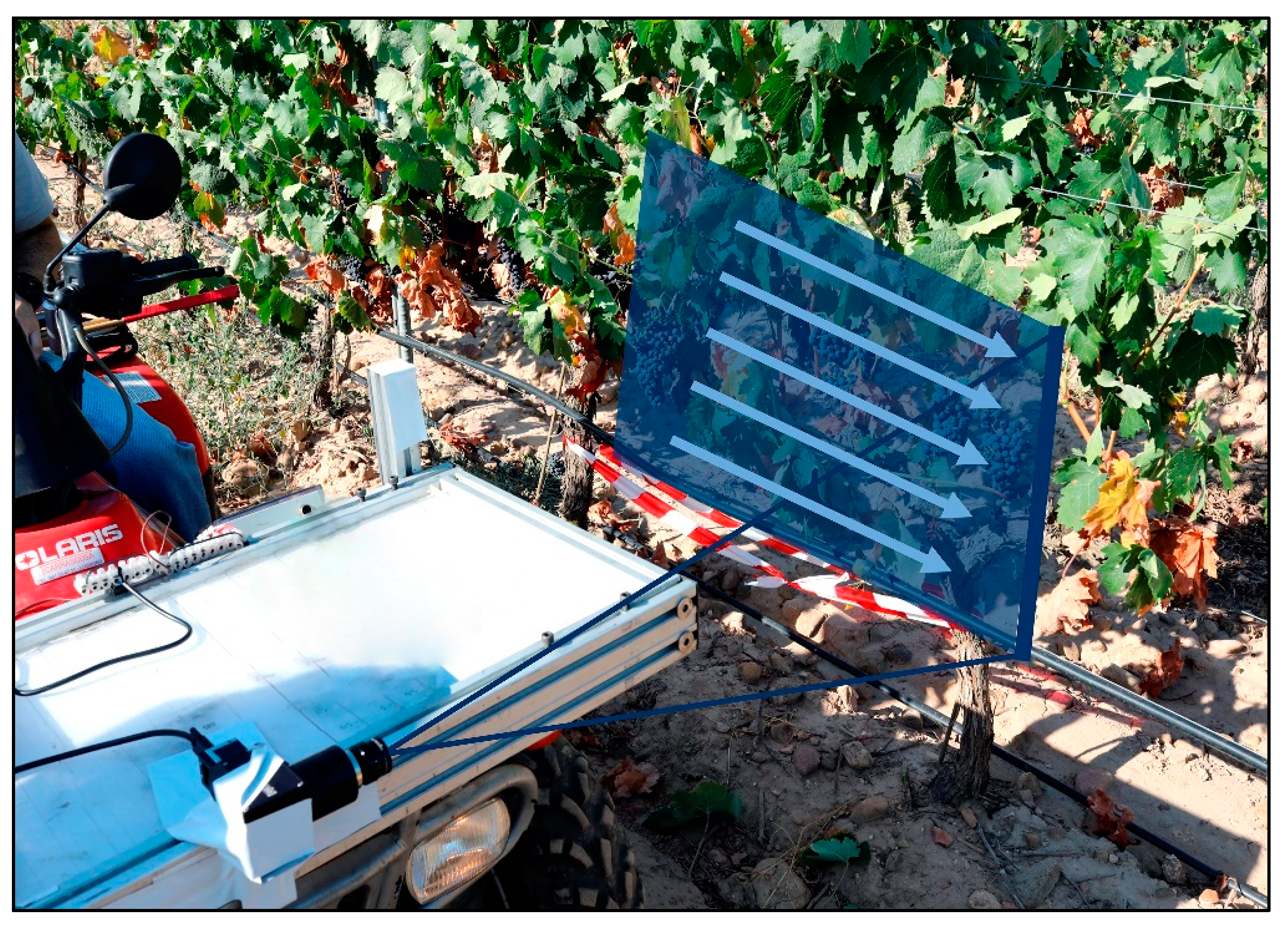
Hyperspectral images were acquired on-the-go using a push broom Resonon Pika L VIS-NIR hyperspectral imaging camera (Resonon, Bozeman, MA, USA) that was mounted in the front part of an all-terrain-vehicle (ATV) (Trail Boss 330, Polaris Industries, Minneapolis, Minnesota, USA) (Figure 1), and connected to an industrial computer also mounted on the ATV. Hyperspectral images were acquired on the east side of the canopy, which was partially defoliated in the basal fruiting zone. Partial defoliation is a common viticultural practice carried out in many wine regions (particularly in cool areas) to promote fruit sun exposure and air circulation.
The spectral resolution of the camera was 2.1 nm (300 bands from 400 to 1000 nm), the amount of information captured by the sensor on each spatial line (column) of the hyperspectral image is 300 pixels. An 8.0 mm focal length lens (field of view of 36.5°) was pointed to the canopy on a lateral point of view at 1.50 m of distance, casting a vertical recording line upon the plants of approximately 0.95 m. The scanning line covered the whole vine canopy, including the fruiting zone (Figure 1).
Each day, a total of 12 hyperspectral images (one for each labelled vine) were acquired on the east side of the canopy, under uncontrolled, natural sun illumination (between 11:00 and 13:00 h). It is necessary to point out, that camera configuration parameters [integration time and frames per second (FPS)] were adapted for each grapevine imaging, depending on the environmental light intensity, in order to find the best trade-off between acceptable image composition, adequate signal to noise ratio, and avoidance of saturation. Frames per second ranged from 100 (taking one frame each 9.8 ms) to 80 (one frame each 12.25 ms) during the experimental trials. Prior to hyperspectral imaging, a Spectralon (Labsphere, Sutton, NH, USA) white reference (a surface with a reflectance over 95%) was manually presented to the camera simulating the same position and distance to the canopy of the grape clusters. The dark current (that corresponds to inherent electronic noise) was measured with the camera lens covered. After this, the grapevine was imaged on-the-go at a constant speed of 5 km/h, composing a hyperspectral image by push broom scanning (Figure 1) with an average number of scanlines of 1.295, with 900 pixels each one. On average, a total of 1.165.000 pixels (i.e., spectra) per plant were acquired.
All the raw information from the camera (acquired as light intensity) was translated into reflectance, using the following equation:
where G is the intensity of the light reflected by the grapevine, W is the intensity of the light coming from the white reference, and D is the dark reference. Afterwards, the reflectance was converted into absorbance [log(1/R)].
2.3. Analysis of Grape Clusters Composition
After on-the-go hyperspectral imaging, a total of 144 clusters (48 clusters per date) were collected and transported to the laboratory of the University of La Rioja in portable refrigerators. Upon arrival to the laboratory, each cluster was weighed, manually destemmed and its berries split into two groups of 100 berries each. The weight of 100 berries was also recorded. When clusters were small (less than 200 berries in total), 50 berries were allocated to each group instead, being sufficient to analyse the composition parameters. The first group of berries was crushed and the must analysed for TSS, pH, Titratable acidity, as well as tartaric and malic acid concentrations. The second set of berries was put in a labelled plastic bag and stored in a freezer at −20 °C until chemical analysis of anthocyanins and total phenols. TSS concentration was determined using a temperature compensating digital refractometer Quick-Brix 60 (Mettler Toledo, LLC, Columbus, OH, USA), expressed as °Brix. Titratable acidity, pH, Tartaric acid and Malic acid were determined following the OIV methods [27]. For the analysis of anthocyanins and total phenols, the berry samples stored at −20 °C were allowed to thaw at 4 °C overnight in a cold room. Samples were taken out of the cold room at least one hour prior to being processed at a temperature between 10–15 °C. Berries were then homogenized using a high-performance disperser T25 Ultra-Turrax (IKA, Staufen, Germany) at high speed (14,000 rpm for 60 s). Subsequently, anthocyanin and total polyphenols were analysed following the Iland method [28]. Anthocyanin concentrations were expressed as mg/fresh berry mass, whereas total polyphenols were expressed as absorbance units (AU) at 280 nm/fresh berry mass.
2.4. Processing of Hyperspectral Images
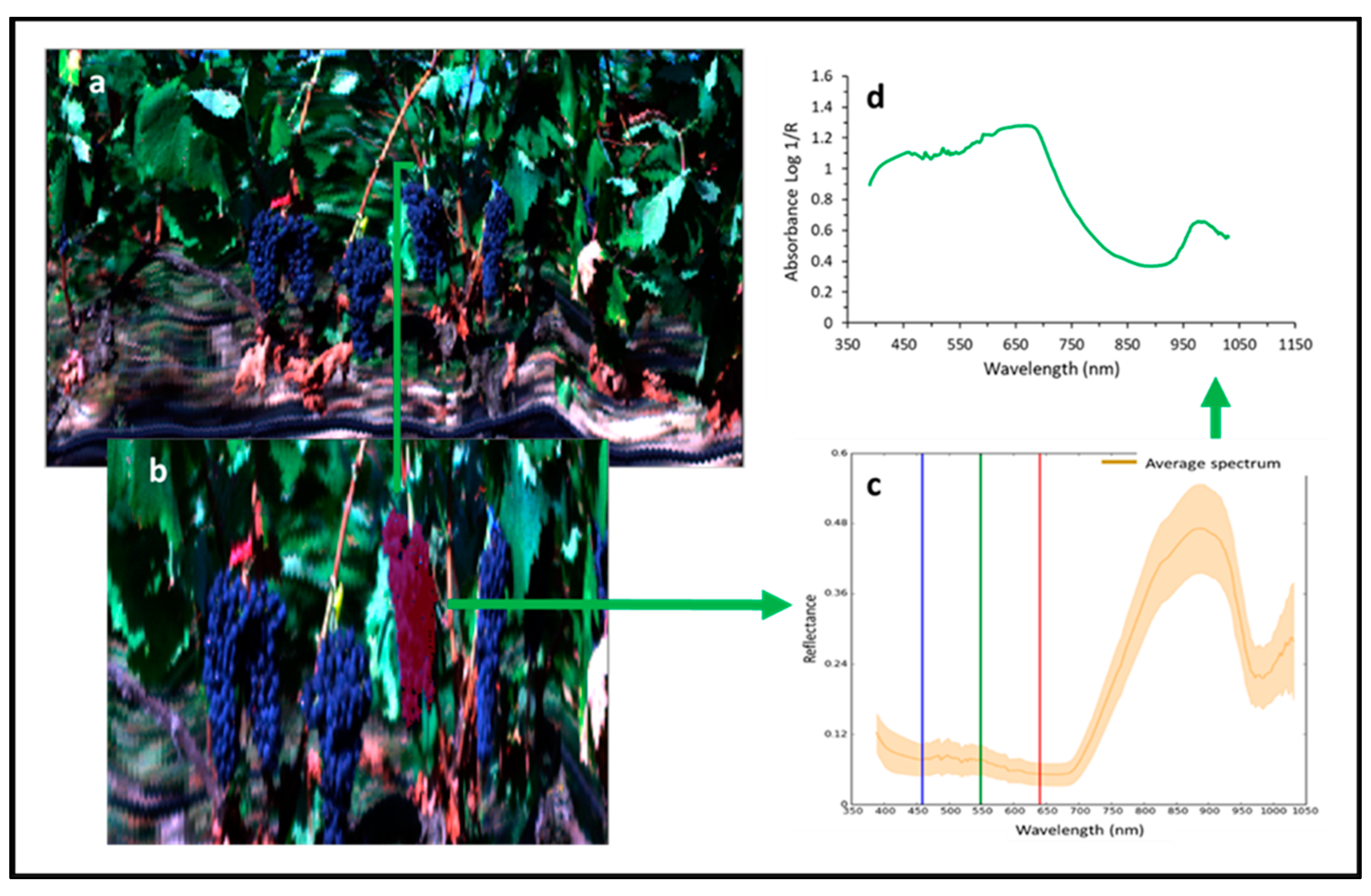
For each hyperspectral image (corresponding to a single grapevine) (Figure 2a) the following process was followed. From the n × m image (where “m” is the number of columns and “n” the number of pixels in each column), four manually selected regions of interest (ROI) corresponding to the four tagged grape clusters were extracted and used to calculate the average spectrum of each grape cluster. Each ROI was created using the “floodfill” tool from the SpectrononPro software (version 5.3, Resonon Inc., Bozeman, MA, USA). This tool allows us to select an adjacent region of pixels with spectral similarity. The “floodfill” tool calculates the Euclidean distance between the clicked pixel and all contiguous pixels and expands the selection to the point at which the selected area contains all of the contiguous pixels for which the spectral distance to the clicked pixel is less than a given tolerance value (Figure 2b). Decreasing the tolerance value, the selected regions were smaller with a greater spectral similarity. In this work, the tolerance value was set to 0.6 as this value was proven to better adjust to the perimeter of the clusters in the images. The mean and standard deviation of the pixels comprised in the ROI were plotted to ensure that the spectral variability remained very similar to the defined grape cluster spectrum (Figure 2c). Finally, the averaged reflectance spectrum for each image was transformed into the corresponding absorbance spectrum (Figure 2d).
2.5. Development of Calibration and Prediction Models
The average spectra of grape clusters were preprocessed to remove the effects of light scattering and to compensate for baseline offset and bias. Several combinations of spectral pre-processing filters were tested and those yielding the best prediction outputs were finally chosen. These filters involved the use of standard normal variate (SNV), detrending (DT) to remove the effects of scattering [29,30], and the application of the Savitzky–Golay smoothing and derivative procedures, selecting distinct values for the window size and degree of the derivative. Derivatives are used to accentuate small bands and to resolve overlapping peaks [31]. Principal component analysis (PCA) was used to explore the data structure, to visualize the presence of spectra outliers and also to identify the main sources of variability in the spectra [32,33]. Spectral data processing and statistical analysis were performed using MATLAB (version 8.5.0, The Mathworks Inc., Natick, MA, USA). PLS-toolbox version 8.1 (Eigenvector Research, Inc., Manson, WA, USA) was used for PCA and PLS regression. This latter algorithm is a widely used chemometric method [34], which has proved to be accurate, robust, and reliable to analyse spectral data, as it is capable of dealing with a vast amount of data, especially when the number of attributes (wavelengths in this case) largely surpasses the number of samples. The input independent variables X were the 300 wavelengths within the spectral range of 400–1000 nm, while TSS, TA, pH, tartaric acid, malic acid, anthocyanins and total polyphenol concentrations were used as dependent variables Y, each one for the training of seven different models. No spectral outliers were detected.
With the aim of building robust models capable of predicting totally unknown samples, the original dataset of 144 samples was split into two independent datasets: a calibration one (comprising 80% or the samples) and a prediction set (with the remaining 20% of the samples), (Table 1). The distribution of the samples into the calibration or prediction subgroup was carried out using the Hotelling’s T2 statistic. This is a measure of the variation in each sample within the PCA model, namely the distance of each sample to the centre of the population. All samples were sorted in reverse order according to the Hotelling’s T2 value. One of every five samples of the original data set was then selected to be part of the prediction set (also called external validation set), which comprised 29 samples. The remaining samples were part of the training set (115 samples). Each set included samples that were appropriately distributed and covered the entire range of each grape composition parameter (Table 1). Once the calibration models were built, cross validation using a 10-fold venetian blind was carried out. In this method, the set of calibration samples was divided into ten subgroups, using one of them to check the results (external validation) and the remaining (nine groups) to build the calibration model. This was repeated as many times as the number of groups (ten in total), in such a way that all the samples were used in both the calibration and external validation subgroups.
For each model, the optimal number of latent variables (LVs) was selected as the one yielding the minimum root mean square error of cross-validation (RMSECV). To appraise the quality of the models, the coefficient of determination (R2) and the root mean square error (RMSE) of calibration (R2c, RMSEC), cross-validation (R2cv, RMSECV), and prediction (R2p, RMSEP) were computed. Additionally, the residual predictive deviation (RPDCV), calculated as the ratio between the standard deviation of the reference data for the training set and the RMSECV was also considered.
The Variable Importance in the Projection (VIP) method [35] was used to identify and evaluate the relative importance of each wavelength in the best grape composition PLS models. VIP score values were computed as the explained sum of squares by the PLS dimension, summed for all dimensions related to the total explained sum of squares by the PLS model and for the total number of wavelengths. Since the average of squared VIP scores is equal to one, influential wavelengths can be considered to be those with VIP scores greater than one [35].
3. Results and Discussion
3.1. Grape Clusters Composition
Table 1 summarizes the descriptive statistics of each grape composition parameter for the whole set of samples (N = 144) as well as for the calibration (N = 115) and external validation (N = 29) sets. Since hyperspectral measurements in the vineyard and corresponding sample collection started early after veraison, and continued until a week before harvest, the value ranges for all compositional variables were wide and representative of berries that were immature to well ripened. Likewise, TSS ranged between 11.10 °Brix to 24.5 °Brix, pH varied between 2.69 and 4.50, TA ranged from 2.20 to 13.40 g/L tartaric acid, malic acid varied from 0.84 to 11.1 g/L, tartaric acid concentration ranged from 4.55 to 12.47 g/L, while anthocyanins and total polyphenols ranged from 0.10 mg/g berry and 0.35 AU/g berry to 2.28 mg/g berry and 2.24 AU/g berry, respectively. It should also be stressed that the structured selection based on the Hotelling’s T2 statistic for the definition of calibration and prediction sets, using only spectral information, displayed similar values for mean, range and standard deviation for all studied grape composition parameters (Table 1), ensuring the suitability of both subsets.
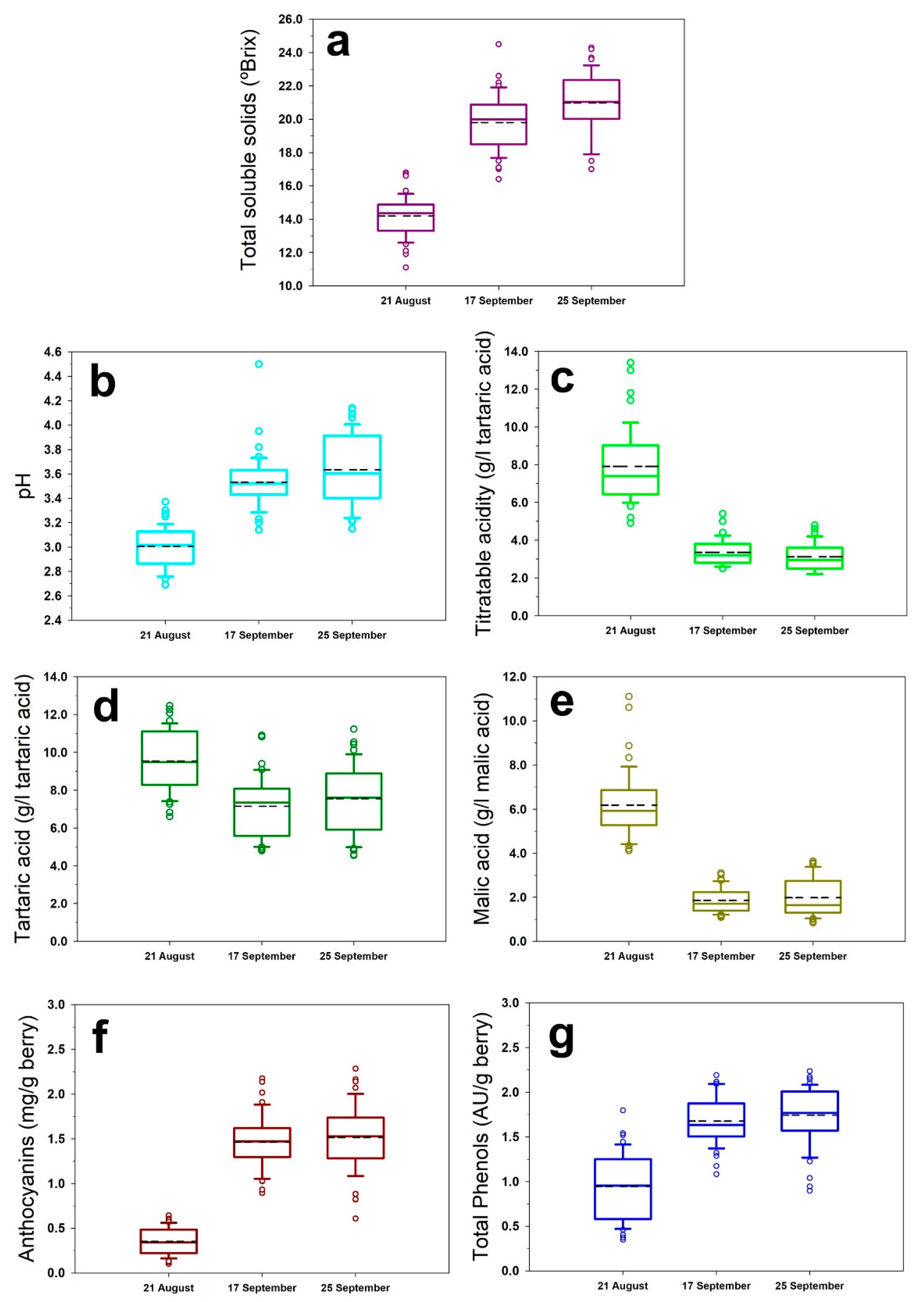
The boxplots of the different grape composition parameters exhibited a normal distribution of data throughout the three days of the study (Figure 3). These boxplots represent the variability of data along the ripening period, with the following statistical metrics: minimum, maximum, median, first and third quartile, and also the mean value of each grape composition parameter for each sampling date. The average TSS and pH (Figure 3a,b) values increased progressively in the studied period, while anthocyanins and total polyphenols (Figure 3f,g) concentrations stabilised in the last two dates.
In terms of the acidity-related parameters, Figure 3c–e illustrates a progressive decline in grape acidity during ripening, as a result of the consumption of malic acid during fruit respiration [36], while the concentration of tartaric acid remains mainly stable, as this organic acid does not catabolize [37]. Malic acid is synthesized following the combustion of sugars in chlorophyll-containing tissues. Unlike tartaric acid, the malic acid is unstable, falling steadily throughout the ripening period (Figure 3f).
3.2. Regression Models for Grape Composition Prediction
Mathematical models were constructed using a PLS algorithm for the predictions of TSS, Titratable acidity, pH, Tartaric acid, Malic acid, Anthocyanins and Total polyphenols’ concentrations. Table 2 lists the performance of the best regression model of calibration, cross-validation, and external validation (prediction) for the quality parameters analysed under field conditions from on-the-go hyperspectral imaging.
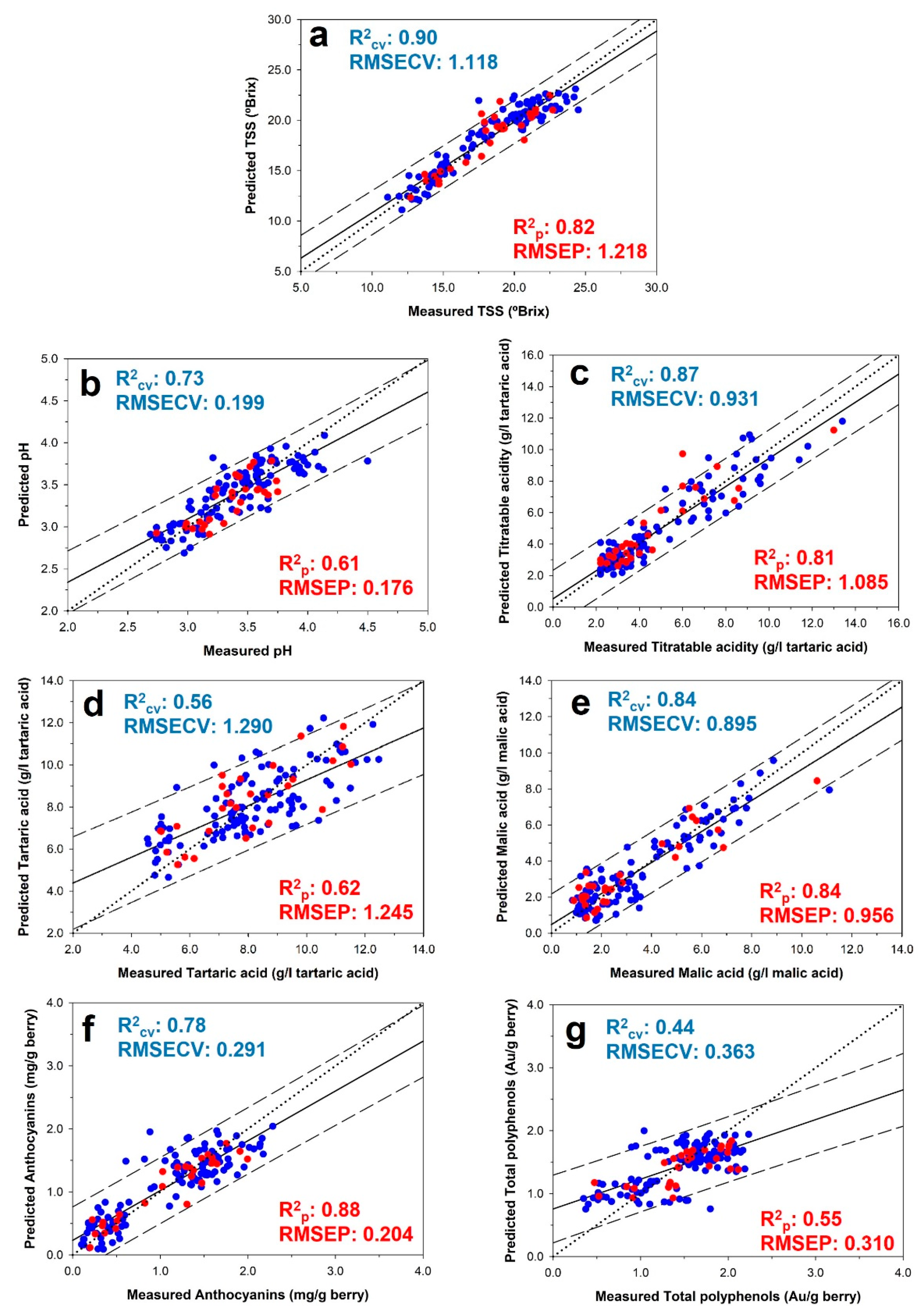
Regarding the spectral preprocessing filters, the best PLS models were yielded only with the application of Savitzky–Golay first derivative and window size of 15. TSS, Titratable acidity and Malic acid returned determination coefficients values of cross (R2cv) and external validation (R2P) close to or above the 0.80 mark for TSS, Titratable acidity, Malic acid and Anthocyanins, respectively (Table 2). Likewise, the RMSECV and RMSEP values were lower or equal to 1.218 °Brix for TSS, 1.085 g/L tartaric acid for Titratable acidity, 0.956 g/L for Malic acid and 0.291 mg/g berry for Anthocyanins. The ratio of performance to deviation values for these four quality attributes analysed were higher than 2.0. The greater the RPD the more accurate is the developed model, and the value of 3 is often assumed as the RPD threshold for screening purposes [33].
However, there are recent works that call for a less categorical use of the RPD, as the information provided by this statistic and that of the determination coefficient (R2) can be similar [38]. Tartaric acid concentration and pH models exhibited more modest values of R2P, above 0.60 and RMSEP, while Total Polyphenols reached R2P of 0.55 and a RMSEP of 0.310 AU/g berry (Table 2). The low number of PLS factors used to build the prediction models (from two factors, for TSS and Total polyphenols, to six factors, such as that of Titratable acidity) ensures that potential overfitting events are minimized and strengthens the robustness and generalization capability of the predictive models.
Figure 4a–g displays the best prediction models for grape composition parameters under field conditions from on-the-go hyperspectral imaging. The samples gathered in the regression plots for TSS (Figure 4a), Titratable acidity (Figure 4c), Malic acid (Figure 4e) and Total Anthocyanins (Figure 4f) show a really good fit along the correlation lines and mostly fitted between the 95% confidence bands. A large data range was covered by the samples from the seven regression models. Figure 4c,e show a better adjustment of the 1:1 line over regression lines (Titratable acidity and Malic acid) than those corresponding to Tartaric acid and total polyphenols regression lines (Figure 4d,g).
Nowadays, most of the studies developed with hyperspectral images to quantify grape composition parameters are performed under controlled conditions (indoor environments) using individual grape berries samples or samples composed of reduced number of grape berries randomly collected from many grape clusters [2,3,39,40,41,42]. In these works, two different spectral ranges (400–1000 nm and 900–1700 nm) were used to determine the grape quality parameters such as Phenolic compounds, TSS, pH, Titratable Acidity and Antioxidant activity. The best prediction results gathered with the PLS regression achieved R2 of 0.86 and standard error of prediction (SEP) values of 2.62 and 3.05 mg/g for Nonacylated and Total Anthocyanins [2,39]; R2 of 0.88, 0.89 and 0.84 and RMSEP values of 0.95 °Brix, 35.6 mg/L and 0.13 g/L CE for TSS, Anthocyanins and Tannins, respectively [3,40,42]. Additionally, in these works, values of R2 of 0.81, 0.78 and 0.62 and RMSEP of 0.25, 0.04 g/100g tartaric acid and 48.98 mg/100g Trolox for pH, Titratable Acidity and Antioxidant Activity, respectively were reported [40,42]. These outcomes are very close to the results presented in this study. It is important to note that, in the present work spectral acquisition was carried out contactless, on-the-go, from a mobile vehicle, and overcoming the difficulties encountered in the vineyard such as irregularities in terrain, vibrations, and differences in the distance between the hyperspectral camera and the target.
Recent works have reported the integration of hyperspectral sensors, global positioning systems (GPS) and a computer unit both on unmanned aerial vehicles [43] and in terrestrial platforms [21] to perform reliable predictions about berry composition. In the latter study, two important parameters (TSS and Anthocyanins) were estimated deploying a VIS–NIR hyperspectral camera mounted on an all-terrain vehicle in a commercial vineyard. In that work [21] the predictive capability of the models trained with support vector machines yielded determination coefficients of prediction R2 of 0.92 and 0.83 with RMSEP values of 1.274 °Brix and 0.211 mg/g berry for TSS and Anthocyanin concentration, respectively. The accuracy of these models was very similar to the ones displayed in this work (RMSEP values of 1.218 °Brix and 0.204 mg/g berry for Anthocyanin). In another study, Benelli et al. (2021) [20] showed the potential of the use of HSI in outdoor conditions, from a manually powered garden cart, towards decision-making about harvest time onset, and the classification of samples of Sangiovese into two classes (ripe vs. unripe) according to the amount of TSS only. The developed models to estimate the TSS concentrations in the berries yielded a R2cv of 0.77 and RMSECV of 0.79 °Brix. It is important to highlight that this work used a manually-powered platform at low speed, which may not be fully suitable to measure large vineyards.
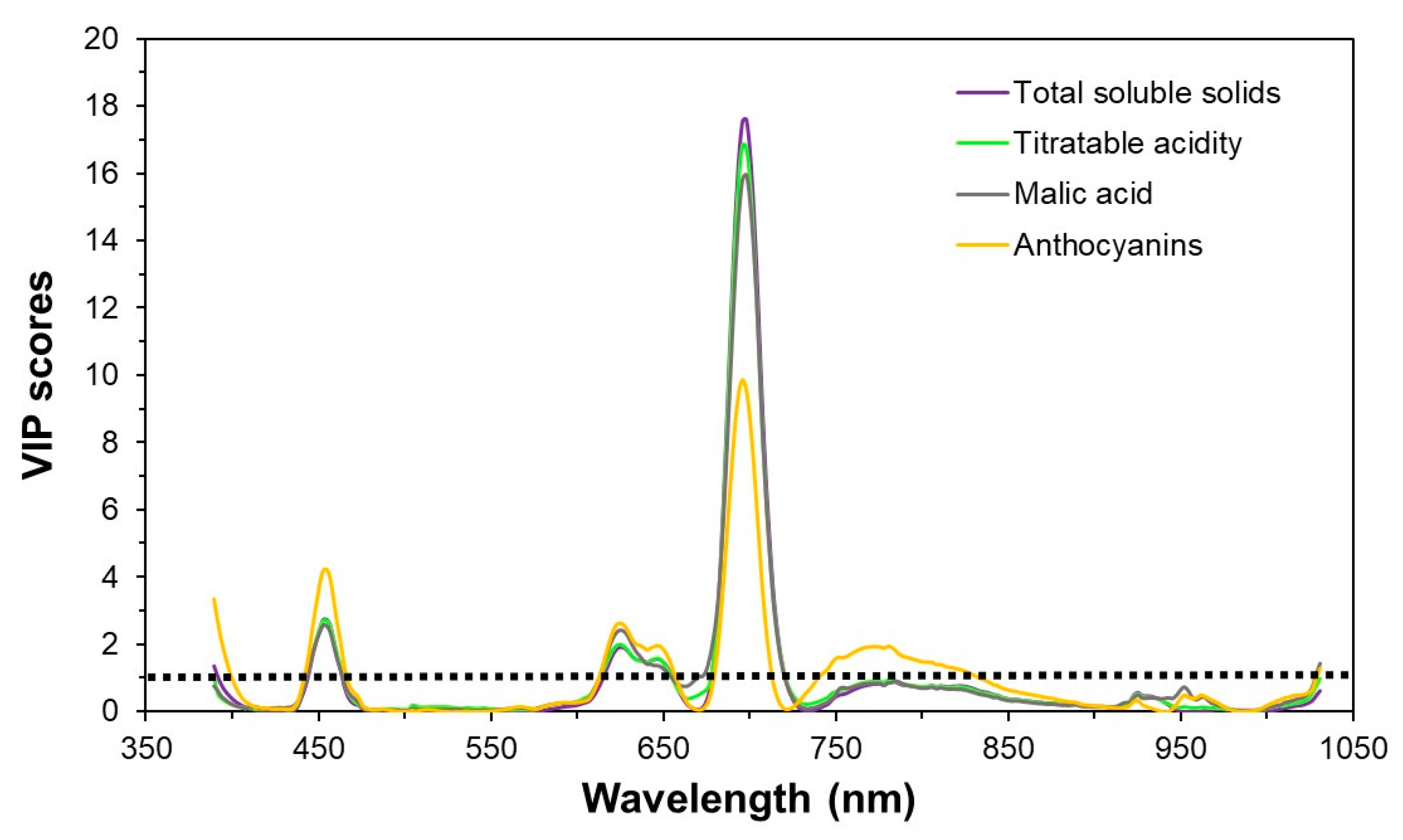
The VIP scores that correspond to the most relevant wavelengths of the best grape composition PLS models (TSS, Titratable acidity, Malic acid and Anthocyanins) are shown in Figure 5. Computation of the VIP scores disclosed the importance of the wavelengths in the Vis region at 454, 625, 646 and 698 nm, with VIP scores above 1. The highest VIP scores for the four quality attributes were observed at 698 nm with VIP values ranging between 9.54 and 17.62. The behaviour of these four parameters was practically the same in terms of the most consistent wavelength, except at around 646 nm, where the trend in the case of Malic acid was different (Figure 5). These findings could pave the way towards a simpler spectral monitoring, from hyperspectral imaging (hundreds of bands) to multispectral imaging (limited number of bands, usually from six to eight), focusing on the spectral acquisition at these four, more informative, wavelengths (454, 625, 646 and 698 nm). Should the performance of the multispectral solution be comparable to that of the hyperspectral camera used in this work, then a lower cost, simpler, easier to process spectral methodology could be used to non-invasively assess the technological maturity (soluble solids and acidity features) and total anthocyanins in grape berries in the vineyard. In fact, this step towards multispectral imaging should be taken in further experimental studies.
The methodology reported in the present work enabled the estimation of the main grape composition parameters, including all relevant acidity variables, whose determination had not been attempted previously, processing the full image of all visible berries associated at each cluster. This approach could ensure that grape monitoring is much more feasible, robust and accurate than those studies in which a few intact berries from the clusters were selected and scanned during the ripening period. The strength and stability of the relationship between the composition of visible berries and that of the entire cluster during ripening was a crucial approach evaluated by Tang et al. [44] as a necessary step towards developing non-destructive, sensing-based systems in the vineyard. These authors reported very good correlations between visible berries and entire clusters, with R2 values ranging from 0.76 to 0.99 for most compositional variables. These findings confirmed the applicability of non-destructive sensing-based systems in the vineyard to assess grape composition evolution during ripening. Moreover, in that study it was also pointed out the need for individual models for different compositional parameters and grape cultivars, as the correlations did not always follow the 1:1 line, as observed as well in the present work. The promising results exposed in this work disclosed a notable methodology on-the-go for the in-field assessment of grape quality composition parameters during the ripening period.
Nevertheless, in this study, grapevines were planted on a vertical trellising, and the fruiting zone was partially defoliated (common practice in many grape-growing regions worldwide), therefore clusters were adequately exposed to the moving hyperspectral monitoring system and the number of fruit-spectra were sufficient in number to the rate of acquisition of the spectral camera and speed at which the ATV moved along the rows. In case of no defoliation at all around the fruiting zone, at least some cluster exposure is necessary since the VIS-NIR radiation cannot go through the leaves completely and reach the clusters behind them. Therefore, in order to expand the applicability of this methodology, it would be necessary to investigate additional factors, such as dissimilar levels of defoliation at the fruiting zone, vineyards planted with different varieties and trellising.
4. Conclusions
This work describes a novel methodology for providing a non-invasive, reliable estimation of the most relevant red berry composition parameters used in grape ripening monitoring, including TSS, acidity features as well as anthocyanins and phenols, using hyperspectral images acquired on-the-go, and subsequently processed to extract the information related to the visible berries from the cluster in VSP Tempranillo (Vitis vinifera L.) vineyards. The results reported in this work confirm the good predictive capacity of the PLS models to track the evolution of the dynamics of the main quality parameters during grape ripening in a commercial vineyard. This approach has the potential to facilitate the decision support process in the field relative to the optimum time for harvesting and selective harvest (according to differences in grape composition) and provides further knowledge about the practical implementation and performance of non-invasive HSI as a helpful technology to be used for monitoring purposes in viticulture in the future.
Author Contributions
Conceptualization, J.F.-N. and M.P.D.; methodology J.F.-N. and M.P.D.; software I.B. and J.F.-N.; validation J.F.-N.; formal analysis I.B., M.P.D. and J.F.-N.; investigation; J.F.-N. and M.P.D.; data curation J.F.-N.; writing—original draft preparation J.F.-N. and M.P.D.; writing—review and editing J.F.-N., I.B. and M.P.D.; supervision M.P.D.; project administration M.P.D. and J.F.-N.; funding acquisition M.P.D.; All authors have read and agreed to the published version of the manuscript.
Funding
This research received no external funding.
Institutional Review Board Statement
Not applicable.
Informed Consent Statement
Not applicable.
Acknowledgments
The authors acknowledge Luis Angel García for his support and Bodegas Vivanco for providing the vineyard to conduct the study. Special thanks to Eugenio Moreda for their help with the analysis of grape cluster composition.
Conflicts of Interest
The authors declare no conflict of interest.
References
- Boulton, R.B.; Singleton, V.L.; Bisson, L.F.; Kunkee, R.E. Principles and Practices of Winemaking; Springer Science & Business Media: Berlin/Heidelberg, Germany, 1996. [Google Scholar]
- Hernández-Fierro, J.M.; Nogales-Bueno, J.; Rodríguez-Pulido, F.J.; Heredia, F.J. Feasibility Study on the Use of Near-Infrared Hyperspectral Imaging for the Screening of Anthocyanins in Intact Grapes during Ripening. J. Agric. Food Chem. 2013, 61, 9804–9809. [Google Scholar]
- Zhang, N.; Liu, X.; Jin, X.; Li, C.; Wu, X.; Yang, S.; Ning, J.; Yanne, P. Determination of total iron-reactive phenolics, anthocyanins and tannins in wine grapes of skins and seeds based on near-infrared hyperspectral imaging. Food Chem. 2017, 237, 811–817. [Google Scholar] [CrossRef]
- Pagay, V.; Cheng, L. Variability in berry maturation of Concord and Cabernet franc in a cool climate. Am. J. Enol. Vitic. 2010, 61, 61–67. [Google Scholar]
- Kliewer, W.M.; Lider, L.A. Influence of cluster exposure to the sun on the composition of Thompson Seedless fruit. Am. J. Enol. Vitic. 1968, 19, 175–184. [Google Scholar]
- Baluja, J.; Diago, M.P.; Balda, P.; Zorer, R.; Meggio, F.; Morales, F.; Tardaguila, J. Assessment of vineyard water status variability by thermal and multispectral imagery using an unmanned aerial vehicle (UAV). Irrig. Sci. 2012, 30, 511–522. [Google Scholar] [CrossRef]
- Beghi, R.; Giovenzana, V.; Marai, S.; Guidetti, R. Rapid monitoring of grape withering using visible near-infrared spectroscopy. J. Sci. Food Agric. 2015, 95, 3144–3149. [Google Scholar] [CrossRef]
- Barnaba, F.E.; Bellincontro, A.; Mencarelli, F. Portable NIR-AOTF spectroscopy combined with winery FTIR spectroscopy for an easy, rapid, in-field monitoring of Sangiovese grape quality. J. Sci. Food Agric. 2014, 94, 1071–1077. [Google Scholar] [CrossRef]
- Herrera, J.; Guesalaga, A.; Agosin, E. Shortwave–near infrared spectroscopy for non-destructive determination of maturity of wine grapes. Meas. Sci. Technol. 2003, 14, 689. [Google Scholar] [CrossRef]
- Urraca, R.; Sanz-Garcia, A.; Tardaguila, J.; Diago, M.P. Estimation of total soluble solids in grape berries using a hand-held NIR spectrometer under field conditions. J. Sci. Food Agric. 2016, 96, 3007–3016. [Google Scholar] [CrossRef]
- Larrain, M.; Guesalaga, A.R.; Agosin, E. A multipurpose portable instrument for determining ripeness in wine grapes using NIR spectroscopy. IEEE Trans. Instrum. Meas. 2008, 57, 294–302. [Google Scholar] [CrossRef]
- González-Caballero, V.; Pérez-Marín, D.; López, M.I.; Sánchez, M.T. Optimization of NIR spectral data management for quality control of grape bunches during on-vine ripening. Sensors 2011, 11, 6109–6124. [Google Scholar] [CrossRef] [Green Version]
- Giovenzana, V.; Civelli, R.; Beghi, R.; Oberti, R.; Guidetti, R. Testing of a simplified LED based vis/NIR system for rapid ripeness evaluation of white grape (Vitis vinifera L.) for Franciacorta wine. Talanta 2015, 144, 584–591. [Google Scholar] [CrossRef]
- Fernández-Novales, J.; Tardáguila, J.; Gutiérrez, S.; Diago, M.P. On-The-Go VIS+ SW- NIR spectroscopy as a reliable monitoring tool for grape composition within the vineyard. Molecules 2019, 24, 2795. [Google Scholar] [CrossRef] [Green Version]
- Grahn, H.; Geladi, P. Techniques and Applications of Hyperspectral Image Analysis; John Wiley & Sons: Hoboken, NJ, USA, 2007. [Google Scholar]
- Gutiérrez, S.; Wendel, A.; Underwood, J. Ground based hyperspectral imaging for extensive mango yield estimation. Comput. Electron. Agric. 2019, 157, 126–135. [Google Scholar] [CrossRef]
- Gutiérrez, S.; Wendel, A.; Underwood, J. Spectral filter design based on in-field hyperspectral imaging and machine learning for mango ripeness estimation. Comput. Electron. Agric. 2019, 164, 104890. [Google Scholar] [CrossRef]
- Wendel, A.; Underwood, J.; Walsh, K. Maturity estimation of mangoes using hyperspectral imaging from a ground based mobile platform. Comput. Electron. Agric. 2018, 155, 298–313. [Google Scholar] [CrossRef]
- Gutiérrez, S.; Fernández-Novales, J.; Diago, M.P.; Tardaguila, J. On-The-Go Hyperspectral Imaging Under Field Conditions and Machine Learning for the Classification of Grapevine Varieties. Front. Plant Sci. 2018, 9, 1102. [Google Scholar] [CrossRef]
- Benelli, A.; Cevoli, C.; Ragni, L.; Fabbri, A. In-field and non-destructive monitoring of grapes maturity by hyperspectral imaging. Biosyst. Eng. 2021, 207, 59–67. [Google Scholar] [CrossRef]
- Gutiérrez, S.; Tardaguila, J.; Fernández-Novales, J.; Diago, M.P. On-the-go hyperspectral imaging for the in-field estimation of grape berry soluble solids and anthocyanin concentration. Aust. J. Grape Wine Res. 2019, 25, 127–133. [Google Scholar] [CrossRef] [Green Version]
- Defilippi, B.G.; Manriquez, D.; Luengwilai, K.; González-Agüero, M. Aroma volatiles: Biosynthesis and mechanisms of modulation during fruit ripening. Adv. Bot. Res. 2009, 50, 1–37. [Google Scholar]
- Chidi, B.S.; Bauer, F.F.; Rossouw, D. Organic acid metabolism and the impact of fermentation practices on wine acidity: A review. S. Afr. J. Enol. Vitic. 2018, 39, 1–15. [Google Scholar] [CrossRef] [Green Version]
- Coombe, B.G. Development and maturation of the grape berry. Aust. NZ Grapegrow. Winemak 1975, 12, 60–66. [Google Scholar]
- Volschenk, H.; Van Vuuren, H.J.J.; Viljoen-Bloom, M. Malic Acid in Wine: Origin, Function and Metabolism during Vinification. S. Afr. J. Enol. Vitic. 2006, 27, 123–136. [Google Scholar] [CrossRef] [Green Version]
- Ribereau-Gayon, P.; Dubourdieu, D.; Donèche, B.; Lonvaud, A. Handbook of Enology: The Microbiology of Wine and Vinifications; John Wiley and Sons Ltd.: Chichester, UK, 2006; Volume 1. [Google Scholar]
- OIV. Compendium of International Methods of Wine and Must Analysis; International Organisation of Vine and Wine: Paris, France, 2009; pp. 154–196. [Google Scholar]
- Iland, P. Chemical Analysis of Grapes and Wine; Patrick Iland Wine Promotions PTYLTD: Athelstone, SA, Australia, 2004. [Google Scholar]
- Dhanoa, M.S.; Lister, S.J.; Barnes, R.J. On the scales associated with near-infrared reflectance difference spectra. Appl. Spectrosc. 1995, 49, 765–772. [Google Scholar] [CrossRef]
- Barnes, R.J.; Dhanoa, M.S.; Lister, S.J. Standard Normal Variate Transformation and De-trending of Near-Infrared Diffuse Reflectance Spectra. Appl. Spectrosc. 1989, 43, 772–777. [Google Scholar] [CrossRef]
- Savitzky, A.; Golay, M.J.E. Smoothing and Differentiation of Data by Simplified Least Squares Procedures. Anal. Chem. 1964, 36, 1627–1639. [Google Scholar] [CrossRef]
- Massart, D.L.; Vandeginste, B.G.M.; Deming, S.N.; Michotte, Y.; Kaufman, L. Data Handling in Science and Technology: Chemometrics a Textbook; Elsevier: Amsterdam, Holland, 1988. [Google Scholar]
- Næs, T.; Isaksson, T.; Fearn, T.; Davies, T. A User Friendly Guide to Multivariate Calibration and Classification; NIR Publications: Chichester, UK, 2002. [Google Scholar]
- Wold, S.; Sjöström, M.; Eriksson, L. PLS-regression: A basic tool of chemometrics. Chemom. Intell. Lab. Syst. 2001, 58, 109–130. [Google Scholar] [CrossRef]
- Wold, S.; Johansson, E.; Cocchi, M. 3d qsar in drug design: Theory, methods and application. In PLS-Partial Least Squares Proj. to Latent Struct; ESCOM: Lieden, The Netherlands, 1993; pp. 523–550. [Google Scholar]
- Peynaud, E. Enología Práctica: Conocimiento y Elaboración del Vino; Mundi-Prensa Libros: Madrid, Spain, 1996. [Google Scholar]
- Burbidge, C.A.; Ford, C.M.; Melino, V.J.; Wong, D.C.J.; Jia, Y.; Jenkins, C.L.D.; Soole, K.L.; Castellarin, S.D.; Darriet, P.; Rienth, M.; et al. Biosynthesis and cellular functions of tartaric acid in grapevines. Front. Plant Sci. 2021, 12, 309. [Google Scholar] [CrossRef]
- Minasny, B.; McBratney, A. Why you don’t need to use RPD. Pedometron 2013, 33, 14–15. [Google Scholar]
- Martínez-Sandoval, J.R.; Nogales-Bueno, J.; Rodríguez-Pulido, F.J.; Hernández-Hierro, J.M.; Segovia-Quintero, M.A.; Martínez-Rosas, M.E.; Heredia, F.J. Screening of anthocyanins in single red grapes using a non-destructive method based on the near infrared hyperspectral technology and chemometrics. J. Sci. Food Agric. 2016, 96, 1643–1647. [Google Scholar] [CrossRef] [Green Version]
- Piazzolla, F.; Amodio, M.L.; Colelli, G. Spectra evolution over on-vine holding of Italia table grapes: Prediction of maturity and discrimination for harvest times using a Vis-NIR hyperspectral device. J. Agric. Eng. 2017, 48, 109–116. [Google Scholar] [CrossRef] [Green Version]
- Diago, M.P.; Fernández-Novales, J.; Fernandes, A.M.; Melo-Pinto, P.; Tardaguila, J. Use of Visible and Short-Wave Near-Infrared Hyperspectral Imaging To Fingerprint Anthocyanins in Intact Grape Berries. J. Agric. Food Chem. 2016, 64, 7658–7666. [Google Scholar] [CrossRef]
- Silva, R.; Gomes, V.; Mendes-Faia, A.; Melo-Pinto, P. Using support vector regression and hyperspectral imaging for the prediction of oenological parameters on different vintages and varieties of wine grape berries. Remote Sens. 2018, 10, 312. [Google Scholar] [CrossRef] [Green Version]
- Vanegas, F.; Bratanov, D.; Powell, K.; Weiss, J.; Gonzalez, F. A novel methodology for improving plant pest surveillance in vineyards and crops using UAV-based hyperspectral and spatial data. Sensors 2018, 18, 260. [Google Scholar] [CrossRef] [PubMed] [Green Version]
- Tang, J.; Petrie, P.R.; Whitty, M. Modelling relationships between visible winegrape berries and bunch maturity. Aust. J. Grape Wine Res. 2018, 116–126. [Google Scholar] [CrossRef] [Green Version]
Figure 1.
Hyperspectral imaging acquired on-the-go with a push-broom camera mounted on an all-terrain vehicle (ATV) at 5 km/h.
Figure 1.
Hyperspectral imaging acquired on-the-go with a push-broom camera mounted on an all-terrain vehicle (ATV) at 5 km/h.

Figure 2.
(a) Hyperspectral image from a grapevine in red, green and blue (RGB) channels; (b) Manual ROI selection using the floodfill tool from SpectrononPro software with a tolerance value of 0.6; (c) Reflectance values of mean and standard deviation of all pixels collected in the grape cluster ROI; (d) Average reflectance spectrum of a grape cluster transformed into the absorbance spectrum.

Figure 3.
Box plots for Total soluble solids (a), pH (b), Titratable acidity (c), Tartaric acid (d), Malic acid (e), Anthocyanins (f) and total polyphenols (g) during the three days of the experimental study. Dashed lines represent mean values.
Figure 3.
Box plots for Total soluble solids (a), pH (b), Titratable acidity (c), Tartaric acid (d), Malic acid (e), Anthocyanins (f) and total polyphenols (g) during the three days of the experimental study. Dashed lines represent mean values.

Figure 4.
Regression plots for Total soluble solids (a), pH (b), Titratable acidity (c), Tartaric acid (d), Malic acid (e), Anthocyanins (f) and total polyphenols (g) using the best Partial Least Squares (PLS) models generated from on-the-go grape clusters hyperspectral images. (blue colour) 10-fold cross validation; (red colour) external validation. Solid line represents the regression line and dotted line refers to the 1:1 line. Prediction confidence bands are shown at a 95% level (dashed lines).

Figure 5.
Variable Importance in the Projection (VIP) score values for the PLS models to determine Total soluble solids (purpura color), Titratable acidity (light green color), Malic acid (gray color), and Anthocyanins (yellow color). The dotted line at VIP value equal to 1 refers to the threshold defined to assess the relevance of each wavelength.


Table 1.
Descriptive statistics of grape composition parameters.
| Data Set | Calibration Set | External Validation (Prediction) Set | |||||||||||||
|---|---|---|---|---|---|---|---|---|---|---|---|---|---|---|---|
| Compound | N | Minimum | Maximum | Mean | SD | N | Minimum | Maximum | Mean | SD | N | Minimum | Maximum | Mean | SD |
| Total soluble solids (°Brix) | 144 | 11.10 | 24.50 | 18.33 | 3.35 | 115 | 11.10 | 24.50 | 18.38 | 3.47 | 29 | 12.70 | 22.70 | 18.11 | 2.79 |
| Titratable acidity (g/L tartaric acid) | 144 | 2.20 | 13.40 | 4.81 | 2.53 | 115 | 2.20 | 13.40 | 4.83 | 2.57 | 29 | 2.20 | 13.00 | 4.73 | 2.39 |
| pH | 144 | 2.69 | 4.50 | 3.39 | 0.36 | 115 | 2.69 | 4.50 | 3.40 | 0.38 | 29 | 2.74 | 3.75 | 3.36 | 0.25 |
| Tartaric acid (g/L tartaric acid) | 144 | 4.55 | 12.47 | 8.09 | 1.93 | 115 | 4.55 | 12.47 | 8.12 | 1.93 | 29 | 4.99 | 11.52 | 7.96 | 1.93 |
| Malic acid (g/L malic acid) | 144 | 0.84 | 11.10 | 3.34 | 2.27 | 115 | 0.84 | 11.10 | 3.40 | 2.25 | 29 | 0.90 | 10.61 | 3.10 | 2.31 |
| Anthocyanins (mg/g berry) | 144 | 0.10 | 2.28 | 1.11 | 0.60 | 115 | 0.10 | 2.28 | 1.11 | 0.62 | 29 | 0.20 | 2.00 | 1.11 | 0.56 |
| Total polyphenols (Au/g berry) | 144 | 0.35 | 2.24 | 1.46 | 0.48 | 115 | 0.35 | 2.24 | 1.44 | 0.49 | 29 | 0.47 | 2.12 | 1.51 | 0.44 |
N: Number of samples; SD: standard deviation.
Table 2.
Calibration, cross-validation, and external validation (prediction) of the best models obtained to predict the grape composition parameters under field conditions from on-the-go Hyperspectral imaging.
Table 2.
Calibration, cross-validation, and external validation (prediction) of the best models obtained to predict the grape composition parameters under field conditions from on-the-go Hyperspectral imaging.
| Calibration | Cross-Validation | External Validation | ||||||||||
|---|---|---|---|---|---|---|---|---|---|---|---|---|
| Parameters | Spectral Treatment | N | SD | Range | PLS Factor | RMSEC | R2c | RMSECV | R2cv | RPD | RMSEP | R2p |
| Total soluble solids (°Brix) | D1W15 | 115 | 3.471 | 11.10–24.50 | 2 | 1.073 | 0.90 | 1.118 | 0.90 | 3.00 | 1.218 | 0.82 |
| Titratable acidity (g/L tartaric acid) | D1W15 | 114 | 2.570 | 2.20–13.40 | 6 | 0.796 | 0.90 | 0.931 | 0.87 | 2.72 | 1.085 | 0.81 |
| pH | SNV + DT D1W15 | 115 | 0.378 | 2.69–4.50 | 4 | 0.180 | 0.77 | 0.199 | 0.73 | 1.81 | 0.176 | 0.61 |
| Tartaric acid (g/L tartaric acid) | D2W15 | 115 | 1.934 | 4.55–12.47 | 5 | 1.108 | 0.67 | 1.290 | 0.56 | 1.50 | 1.245 | 0.62 |
| Malic acid (g/L malic acid) | D1W15 | 115 | 2.253 | 0.84–11.10 | 5 | 0.784 | 0.88 | 0.895 | 0.84 | 2.55 | 0.956 | 0.84 |
| Anthocyanins (mg/g berry) | SNV + DT D1W15 | 115 | 0.615 | 0.10–2.28 | 3 | 0.275 | 0.80 | 0.291 | 0.78 | 2.06 | 0.204 | 0.88 |
| Total polyphenols (Au/g berry) | D1W15 | 115 | 0.485 | 0.35–2.24 | 2 | 0.343 | 0.50 | 0.363 | 0.44 | 1.32 | 0.310 | 0.55 |
DnWm: Savitzky–Golay filter with n-degree derivative, window size of m. SNV + DT: standard normal variate plus detrending. N: number of samples used for calibration and cross-validation models after outlier detection. SD: standard deviation. RMSEC: root mean square error of calibration. R2c: determination coefficient of calibration. RMSECV: root mean square error of cross-validation. R2cv: determination coefficient of cross-validation. RPD: residual predictive deviation. RMSEP: root mean square error of prediction. R2p: determination coefficient of prediction.
Publisher’s Note: MDPI stays neutral with regard to jurisdictional claims in published maps and institutional affiliations. |
© 2021 by the authors. Licensee MDPI, Basel, Switzerland. This article is an open access article distributed under the terms and conditions of the Creative Commons Attribution (CC BY) license (https://creativecommons.org/licenses/by/4.0/).
Share and Cite
MDPI and ACS Style
Fernández-Novales, J.; Barrio, I.; Diago, M.P. Non-Invasive Monitoring of Berry Ripening Using On-the-Go Hyperspectral Imaging in the Vineyard. Agronomy 2021, 11, 2534. https://doi.org/10.3390/agronomy11122534
AMA Style
Fernández-Novales J, Barrio I, Diago MP. Non-Invasive Monitoring of Berry Ripening Using On-the-Go Hyperspectral Imaging in the Vineyard. Agronomy. 2021; 11(12):2534. https://doi.org/10.3390/agronomy11122534
Chicago/Turabian StyleFernández-Novales, Juan, Ignacio Barrio, and María Paz Diago. 2021. "Non-Invasive Monitoring of Berry Ripening Using On-the-Go Hyperspectral Imaging in the Vineyard" Agronomy 11, no. 12: 2534. https://doi.org/10.3390/agronomy11122534
Note that from the first issue of 2016, this journal uses article numbers instead of page numbers. See further details here.