Total and Hot-Water Extractable Organic Carbon and Nitrogen in Organic Soil Amendments: Their Prediction Using Portable Mid-Infrared Spectroscopy with Support Vector Machines

Abstract

Against the background of climate change mitigation, organic amendments (OA) may contribute to store carbon (C) in soils, given that the OA provide a sufficient stability and resistance to degradation. In terms of the evaluation of OA behavior in soil, total organic carbon (TOC), total nitrogen (TN), and the ratio of TOC to TN (CN-ratio) are important basic indicators. Hot-water extractable carbon (hwC) and nitrogen (hwN) as well as their ratios to TOC and TN are appropriate to characterize a labile pool of organic matter. As for quickly determining these properties, mid-infrared spectroscopy (MIRS) in combination with calibrations based on machine learning methods are potentially capable of analyzing various OA attributes. Recently available portable devices (pMIRS) might replace established benchtop devices (bMIRS) as they have potential for on-site measurements that would facilitate the workflow. Here, we used non-linear support vector machines (SVM) to calibrate prediction models for a heterogeneous dataset of greenwaste composts and biochar compost substrates (BCS) (n = 45) using bMIRS and pMIRS instruments on ground samples. Calibrated models for both devices were validated on separate test sets and showed similar results. Ten OA were sieved to particle size classes (psc’s) of >4 mm, 2–4 mm, 0.5–2 mm, and <0.5 mm. A universal SVM model was then developed for all OA and psc’s (n = 162) via pMIRS. Validation revealed that the models provided reliable predictions for most parameters (R² = 0.49–0.93; ratio of performance to interquartile distance (RPIQ) = 1.19–5.70). We conclude that (i) the examined parameters are sensitive towards chemical composition of OA as well as particle size distribution and can therefore be used as indicators for labile carbon and nitrogen pools of OA, (ii) prediction models based on SVM and pMIRS are a feasible approach to predict the examined C and N pools in organic amendments and their particle size class, and (iii) pMIRS can provide valuable information for optimized application of OA on cultivated soils at low costs and efforts.

1. Introduction

Organic amendments such as compost and biochar products play a key role in maintaining adequate soil organic matter (SOM) levels and thus soil fertility in agriculture and viticulture. The incorporation of organic amendments (OA) into soils can have various positive effects on chemical and physical soil properties such as reduced soil compaction and erosion [1], enhanced nutrient availability, or water-holding capacity [2,3]. Against the background of climate change mitigation, such amendments may also contribute to store carbon (C) in soils as organic C can be bound to clay minerals [4] and have a high recalcitrance against microbial degradation [5]. Yet, the composition of the OA incorporated in soils is a fundamental key to whether the applied C can be stored or is predominantly mineralized by microorganisms [6], which would cause higher emission of greenhouse gasses such as CO₂ and N₂O [7]. Rapid turnover would therefore be detrimental to the climate change goals, e.g., of the COP21 of Paris (https://www.un.org/en/climatechange/paris-agreement (accessed on 29 March 2021)), and therefore needs to be determined before OA are incorporated into soils. Two kinds of substrates are the focus of this study, namely, greenwaste composts and biochar compost substrates (BCS). Adding biochar to composts can be of special interest for carbon storage in soils because the pyrolysation process results in a product with a high amount of stable C and can thus reduce the emission of greenhouse gases [8]. Further, this mixture has been reported to benefit plant growth by enhancing water holding capacity and nutrient cycling [9,10] and to reduce erosion by improving soil structure [11]. Yet, the relatively high costs for such products suggest application in orchards or viticulture rather than in arable farming (which is the background of this study).

As a consequence of different material origin and material treatment during the production process, organic C and N pools of compost and BCS products can vary in their chemical composition and particle size distribution. Both can affect potential carbon turnover in soils [12]. Chemical composition can be characterized by the determination of total organic carbon (TOC) and total nitrogen (TN) and the respective CN ratios. Although these factors are important for C turnover, more detailed information about C and N composition is necessary to determine potential greenhouse gas emissions by OA. Hot water extraction has shown to be a sensitive indicator for labile C and N pools (hot-water extractable carbon (hwC), hot-water extractable nitrogen (hwN)) [13,14,15]. Other work showed a strong correlation of hwC to CO₂ development in soils [16], indicating that hwC also is likely to be easily available for microbial processing. Further, hwC has been reported as a parameter that decreases during the decomposition process, and has therefore been related to the process of C-stabilization [17]. Another important pool is hwN, a parameter for labile N, easily available for plants after transformation to mineral N [18,19]. As a consequence, hwC and hwN are promising indicators for the determination of C stability in different OA. Further, calculating the proportion of hwC to TOC (hwC_prop) and hwN to TN (hwN_prop) can provide valuable information about C and N stability in OA. A high proportion of the hw-pool to the total pool would therefore indicate lower C stability and vice versa. Yet these laboratory methods are still time-, labor-, and resource-consuming. Thus, for a rapid determination of these compounds, new methods need to be approached to overcome these obstacles and to facilitate future research.

Mid-infrared spectroscopy (MIRS) is increasingly being used for the fast determination of chemical soil parameters [20,21,22,23]. Optic instruments such as MIRS have great potential to reduce laborious efforts, because various sample properties can be derived from a single spectrum and analytical labor can be minimized after model calibration, thus making infrared spectroscopy more cost- and time-efficient. Recently, portable MIR (pMIRS) instruments became available and are increasingly being used by scientists as they provide the potential for on-site measurements. Comparisons of a pMIRS to an established benchtop device showed similar results for calibration models predicting soil organic carbon [24,25,26]. Yet these studies focused on soil samples and research regarding pMIRS on OA properties is still scarce.

For the prediction of sample properties via pMIRS, statistical models need to be calibrated. Calibration requires conventionally analyzed samples prior to predicting properties of unknown samples. In a partial least squares regression (plsr) approach, the authors of [27] used benchtop MIRS (bMIRS) to predict organic carbon and total nitrogen in compost and organic waste products, and the authors of [28] used bMIRS to predict humic acids as well as respiration activity to determine compost quality. Calibrated models provided convenient results for these parameters. However, these studies did not aim at combining various compost and BCS amendments in one prediction model. Moreover, the spectral response of OA can vary widely and limit the performance of linear models such as plsr because factors such as material origin, particle size distribution, fermentation conditions, or pyrolytic decomposition during biochar production and therefore the chemical composition during biochar production vary to a high degree. A computational approach to overcome these interfering influences is the use of machine learning methods [29]. Because of their ability to determine complex and non-linear relationships, these methods became popular in several research fields. For this study, support vector machines (SVM) were of special interest. They are a non-parametric, non-linear statistical learning method that does not assume a known statistical distribution of the data [30]. This supervised machine learning method was initially developed for classification of linearly separable classes of objects by a hyperplane [31]. However, SVM can also be a powerful tool for predictive regression modeling when classes of objects cannot be separated with a linear classifier. The coordinates of the objects are rearranged in a higher dimensional feature space with up to infinite dimensions [32]. For computation of the classification hyperplane in a high-dimensional feature space, so-called kernels are used. Kernels are mathematical functions that move the data in the feature space while operating in the input space. Further, SVM are capable of handling rather small training datasets [33] while maintaining a high generalization potential for unknown (test) data [30]. Finally, they provide robustness to (spectral) outliers [34]. In this context, pMIRS in combination with SVM regression seems promising for the determination of organic C and N pools in OA and their particle size classes (psc’s).

The aims of this study were (i) to identify variation of C and N pools and their particle size distribution in differing OA, and (ii) to develop a prediction model for C and N pools using pMIRS via SVM. First, we analyzed the ground truth data of the OA regarding C and N pools; second, we calibrated predictive models for these C and N pools using pMIRS and bMIRS via SVM; and third, we calibrated prediction models using pMIRS and SVM including differing OA and psc’s in one model.

2. Materials and Methods

2.1. Organic Amendments

The sample set comprised 15 OA, thereof 12 greenwaste composts and 3 biochar compost substrates (BCS) that were all designated for application in German vineyards. The greenwaste composts were supplied by the Bundesgütegemeinschaft Kompost e.V. (Cologne, Germany) and originated from different recycling facilities in North Rhine-Westphalia and Rhineland-Palatinate (Germany). The commercial BCS products were provided by Palaterra GmbH (Hengstbacherhof, Germany).

Before further processing, all OA were dried at 40 °C. The materials were obviously heterogeneous, i.e., particle size distribution varied between the materials. Therefore, 8 selected composts and 2 BCS were fractionated to size classes of <0.5, 0.5–2, 2–4, and >4 mm to examine potential differences in the amounts of C and N pools related to differing particle size (subset “psc”). The dry weight fraction of each psc from the total material is given in

Table 1. Weight proportions (g kg⁻¹) from the particle size classes (psc’s) of the materials.

Substrate	>4 mm	2–4 mm	2–0.5 mm	<0.5 mm
Compost 1	304	201	326	169
Compost 2	105	89	348	459
Compost 3	225	190	400	184
Compost 4	407	221	265	106
Compost 5	243	162	357	238
Compost 6	295	157	279	26.9
Compost 7	375	180	302	142
Compost 8	603	108	157	132
BCS 1	102	223	468	207
BCS 2	150	152	526	173

.

The fractionated materials were trifold independently sampled for subsequent analyses. Furthermore, we included the integer (unfractionated) samples of all OA under study. The entire sample set under study can be seen in

Table 2. Number of fractionated and unfractionated samples of compost and biochar compost substrates (BCS) materials.

Substrate	Unfractionated	<0.5 mm	0.5–2 mm	2–4 mm	>4 mm	Total
Compost	36	24	24	24	21	129
BCS	9	6	6	6	6	33
Total	45					162

. Finally, all samples were ground in a ball mill to standardize surface conditions for MIRS and analytical measurements.

2.2. Determination of Laboratory Data

Determination of hwC and hwN followed the method of [13] and was carried out by a 1-h extraction of 5 g OA and 25 mL distilled water at 100 °C under reflux. After extraction, cooling, filtration, and centrifugation at 2600 min⁻¹ for 10 min, the dissolved organic carbon and nitrogen in the supernatant were analyzed with a TOC analyzer (Shimadzu TOC-VCPA; Shimadzu Deutschland GmbH, Duisburg, Germany). For each sample, 3 repeated measurements were carried out.

Total organic carbon was determined from the difference between total carbon and inorganic carbon. Total carbon and TN were determined by dry combustion and elemental analysis (ISO 10694, 1995) by 2 repeated measurements. If present, inorganic carbon was determined by the gas-volumetric Scheibler Method (ISO 10693). Otherwise, if no inorganic carbon was present, total carbon was rated as TOC for further analyses.

2.3. Acquisition of Benchtop and Portable MIR Spectra

For bMIRS, about 20 mg of the ground sample was divided into 5 repetitions into the hollowed positions of a microtiter plate and smoothed with a plunger. Diffuse reflectance mid-infrared Fourier transform (DRIFT) spectra were recorded in the laboratory with a Bruker Tensor 27 HTS-XT for automated high-throughput screening (Bruker Optik, Ettlingen, Germany). The device is operated with a liquid N₂ cooled mercury cadmium telluride detector and a broadband KBr beam splitter (Figure 1a). Spectra acquisition was carried out with 120 scans at a resolution of 4 cm⁻¹ and a spectral range of 7500–550 cm⁻¹.

For pMIRS measurements, a handheld FTIR Agilent 4300 (Agilent Technologies, Santa Clara, CA, USA) equipped with a deuterated triglycine sulfate (DTGS) detector and a zinc selenide beam splitter, a DRIFT interface, and a golden reference cap was used (Figure 1b). For spectra acquisition, 2 g of each ground sample was placed in a Petri dish and smoothed by gentle pressing. For each sample, 3 repeated measurements were carried out after slightly rotating the Petri dish between the measurements. Each spectrum was recorded with 80 scans, as previous tests had shown no reduction in standard deviation of the spectra with 100 and 120 scans, respectively. Spectra acquisition with pMIRS was carried out on an instrument stand provided by the manufacturer (Figure 1b). Spectra with the portable device were collected in the 4000–650 cm⁻¹ range and a spectral resolution of 4 cm⁻¹. For compensation of instrument drift and variation in the environment of the measuring chamber, a background spectrum was taken every 10 min using a golden reference cap. The comparison of predictive models gained by bMIRS and pMIRS was performed as a preliminary test on the unfractionated dataset (n = 45, Table 2). For further investigation of pMIRS spectra, the entire dataset, including psc’s, was used for model calibration and validation (n = 162, Table 2).

2.4. Spectra Pre-Treatment and SVM Model Calibration

For further analysis, the spectra of each sample were averaged in order to reduce noise. Model calibrations were done using the spectral range of 3800–650 cm⁻¹ from both instruments. Spectral pre-treatment and SVM model calibration were done with the statistic software R (2013) using the packages: “e1701” [35], “prospectr” [36], and “ggplot2” [37] for visualization. Eight pre-treatments of absorbance spectra were selected to remove light scattering effects, to correct baseline offset, and to improve model performance: no pre-treatment, multiplicative scatter correction (MSC), Savitzky Golay Filter (SG), SNV Standard Normal Variate-Detrend algorithm (SNV), first derivation (1st der), first derivation + SG (1st der + SG), second derivation (2nd der), second derivation + SG (2nd der + SG). These preprocessing approaches were evaluated by the associated cross-validation results and the best model was finally chosen. Prior to model calibration and to avoid overfitting of calibrated models, the 2 different sample sets (Table 2) were divided into independent calibration (70%) and validation (30%) samples by using the k-means sampling algorithm [38]. For an optimal distribution of calibration and validation set, the k-means sampling algorithm was run with 100 iterations. For the non-linear SVM approach in this study, we used the radial basis function kernel for model calibration. Some general information about the SVM approach is outlined in the Introduction section; for a more detailed explanation of SVM, see [31,39,40]. The SVM prediction models were trained using repeated 10-fold cross validation for all spectral pre-treatments in order to find the optimal prediction model for each investigated parameter. Cross-validation was optimized by an automated grid search for the SVM hyperparameters gamma (γ) and cost. The range for both hyperparameters was set to 0.1, 0.5, 1, 5, 10, 25, 50, and 100. Then, a test set validation was performed to test the model performance on “unknown” data. To determine the quality of the predictive models, we used the coefficient of determination of cross validation (R²_CV), the coefficient of determination of prediction (R²_pr; for test set validation), root mean squared error of cross validation (RMSE_CV), root mean squared error of prediction (RMSE_Pr), the ratio of performance to interquartile distance of cross validation (RPIQ_cv), and the ratio of performance to interquartile distance of prediction (RPIQ_pr) according to [41], and calculated it as follows:

$$\mathrm{RMSE}=\sqrt{\frac{1}{\mathrm{n}}{\displaystyle \sum }_{\mathrm{i}=1}^{\mathrm{n}}{\left(\mathrm{fi}-\mathrm{yi}\right)}^2}$$

(1)

where $\mathrm{fi}$ is the predicted, and $\mathrm{yi}$ the respective observed value, and

$$\mathrm{RPIQ}=\frac{\mathrm{IQ}}{\mathrm{RMSE}}$$

(2)

where IQ is the interquartile distance that gives the range that accounts for 50% of the population around the median.

For RPIQ values, the threshold for an unsuccessful model performance was defined by RPIQ < 1.89 according to [42]. Nevertheless, the authors stated that the usefulness of a model should additionally by evaluated in its specific context.

3. Results and Discussion

With respect to fundamental differences between composts and BCS in some of the properties under study, the OA were grouped as such in the following section.

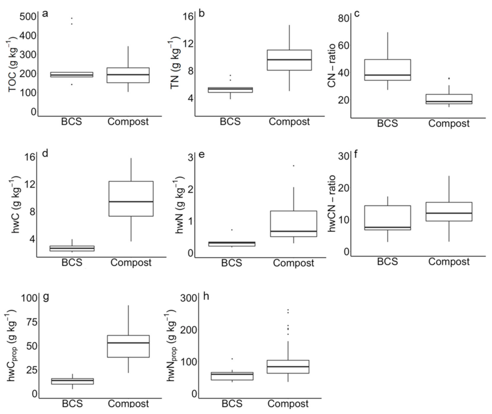
3.1. Laboratory Analysis

The results of the laboratory analyses are displayed as boxplots where the lower and upper hinges correspond to the first and third quartiles, respectively, while the line in between marks the median. The whiskers extend no further than the largest or smallest value of 1.5 * interquartile range from the hinges. Values beyond the end of the whiskers are marked as outliers.

Overall, BCS products tended to equal TOC, lower TN, and higher CN values than composts, yet had notably less hwC (Figure 2a–d). This further resulted in lower hwC_prop values for BCS. As hwC is considered to contain labile C pools [16,43], these results indicate that BCS products might be more suitable in terms of potential soil C-storage.

Other studies found that the addition of biochar to compost products were beneficial for C-sequestration compared to pure compost [44], because biochar has a high recalcitrance and therefore large amounts of stable C as a consequence of the pyrolysation process during biochar production. These results support our assumptions. Nevertheless, samples of both OA types revealed a considerable variation for most C and N pools. In Figure 3a–h, analytical data of four psc’s, ranging from <0.5 mm to >4 mm, is shown. In general, the results of psc fractionation were similar to unfractionated samples. For most examined parameters (e.g., TN, hwC, hwN, hwC_prop, and hwN_prop), psc’s of compost products had higher variations than those of BCS.

High variation of these pools can be considered a consequence of varying raw materials in different production facilities, thus resulting in a diverse chemical composition of the materials and their psc’s under study. For BCS, especially TOC values and variation were larger for the psc > 4 mm compared to the other psc’s of this parameter. Within this psc, the highest visible biochar content was found. As the biochar amount varied between the tested BCS products, this would explain higher TOC values and variation of BCS > 4 mm. This is further supported by lower hwC_prop values for BCS > 4 mm, underlining the higher amount of stable C within biochar [44]. For the other parameters, psc fractionation elevated variation in most parameters compared to the unfractionated samples. In the context of these findings, a quick and precise determination of these pools and therefore C storage potential of OA is desirable.

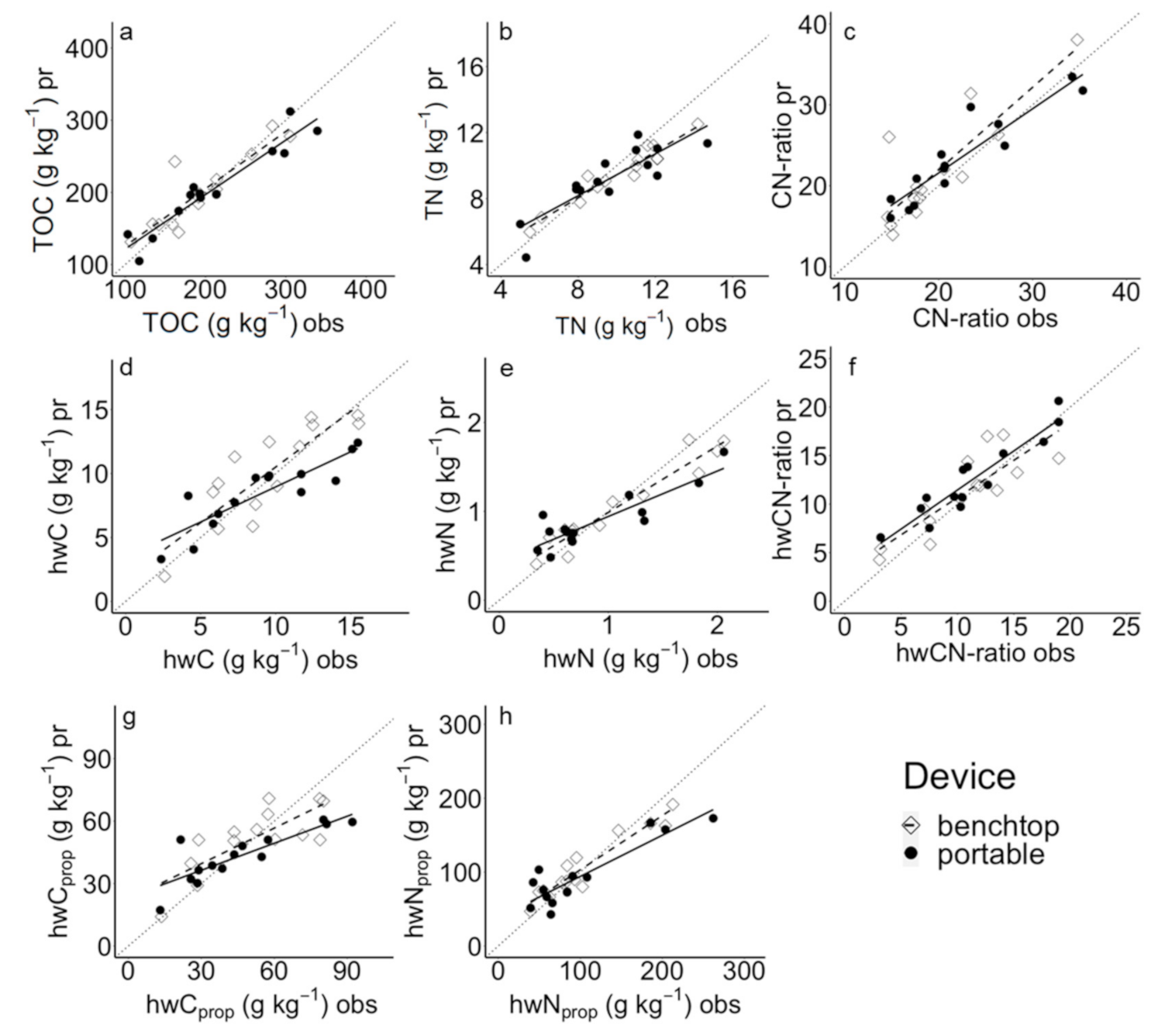
3.2. Comparison of Prediction Models for Integer OA Calibrated on bMIRS and pMIRS Spectra

Portable MIRS combined with SVM was expected to be a promising approach for a quick determination of the above-described C and N pools. Nevertheless, before a more general approach can be addressed, the prediction accuracy of pMIRS was compared to an established benchtop MIRS to justify the use of a portable spectrometer.

When observing the MIRS data within the space of the principal component analysis (PCA), it was evident that spectral information varied between the tested devices, even though spectra were MSC-corrected before PCA to cope with differing measuring conditions (Figure 4a,c). As a consequence, the k-means sampling algorithm chose different spectra for calibration and validation among pMIRS and bMIRS datasets, because it evaluated data on the basis of spectral information within the PC space [38]. The different selection of samples is also reflected in the MSC-corrected MIR spectra in Figure 4b,d. While the shape of pMIRS and bMIRS spectra was generally similar, the spectra obtained with pMIRS revealed higher noise, especially in the region of 3800–3000 cm⁻¹.

The higher noise of the pMIRS spectra was perhaps due to a less reproducible and/or smaller pressure when compacting and smoothing the ground sample in the Petri dishes prior to spectra acquisition. It is proven that surface conditions impact MIR spectra quality [45]. However, the larger quantity of sample material needed for pMIRS made this preparation step particularly challenging. However, the larger noise did not eventually result in worse model accuracy and robustness. The same statement was made by [24,46], although the authors used a plsr method. In this study, SVM model validations revealed corresponding results and proved that modelling coped with different measuring conditions. Within the test set validation, most OA properties were predicted with satisfactory to excellent performance (

Table 3. Test set validation (n = 14) statistics and kernel function hyperparameters gamma (γ) and cost (C) of SVM models for the prediction of compost and BCS properties using a benchtop MIRS (B) and a portable MIRS (P).

Property	Device	Spectral Pre-Treatment	RMSEPr	R2Pr	RPIQPr	γ	C
TOC (g kg−1)	B	1st der + SG	25.8	0.79	2.11	0.5	100
	P	SG	24.8	0.91	3.86	0.1	25
TN (g kg−1)	B	1st der + SG	1.0	0.93	3.11	0.1	25
	P	MSC	1.4	0.73	2.45	0.1	5
CN-ratio	B	MSC	3.96	0.72	1.60	0.1	100
	P	1st der	2.69	0.85	3.03	1	100
hwC (g kg−1)	B	SNV	2.08	0.72	2.75	0.1	10
	P	none	2.28	0.76	2.53	0.1	5
hwN (g kg−1)	B	1st der + SG	0.19	0.93	5.15	1	10
	P	SG	0.30	0.78	2.62	0.5	5
hwCN-ratio	B	1st der	2.43	0.71	2.38	1	100
	P	1st der	2.01	0.88	2.82	1	100
hwCprop (g kg−1)	B	1st der + SG	13.2	0.61	2.75	0.1	100
	P	none	15.0	0.71	1.88	0.1	5
hwNprop (g kg−1)	B	1st der + SG	19.7	0.91	3.52	1	100
	P	1st der	34.7	0.81	1.38	1	100

), wherein R²_pr values ranged from 0.61 (hwC_prop; bMIRS) to 0.93 (TN; bMIRS) and RPIQ_pr from 1.38 (hwN_prop; pMIRS) to 5.15 (hwN; bMIRS). For N pools, bMIRS prediction accuracy of validated models outperformed those of pMIRS with R²_pr of 0.93 (TN), 0.93 (hwN), and 0.91 (hwN_prop). The best bMIRS models listed in Table 3 were all calibrated by pre-treating bMIRS spectra via first derivation and SG smoothing. Yet, RPIQ values for TN and hwN prediction models of pMIRS also indicated good model robustness.

For TOC, TN, and the CN-ratio, the observed and predicted values were consistent and close to the 1:1 line for both devices (Figure 5a–c). Yet pMIRS performed better for TOC and CN-ratios (Table 3). For hwC, the portable device performed slightly better with overall moderate accuracy (R²_pr = 0.76 for pMIRS and 0.72 for bMIRS) (Figure 5d). Even though regression lines for the hwC validation samples differed between the tested MIRS devices, RPIQ_pr values revealed good model robustness for both spectrometers (Table 3). For hwC_prop and hwN_prop of pMIRS models, RPIQ_pr values showed low model robustness and thus a low generalization capacity of SVM models for the prediction of these parameters (Table 3, Figure 5g,h).

While predictive models from bMIRS performed better for N pools, pMIRS models revealed a higher prediction accuracy and model robustness for the C and CN pools. Nevertheless, statistical model parameters for the validation dataset were satisfying for both devices and most parameters. Recent findings of other authors [24,46,47] suggest similar results for soil samples. All in all, pMIRS is considered a reliable alternative to benchtop devices for the prediction of C and N parameters of OA.

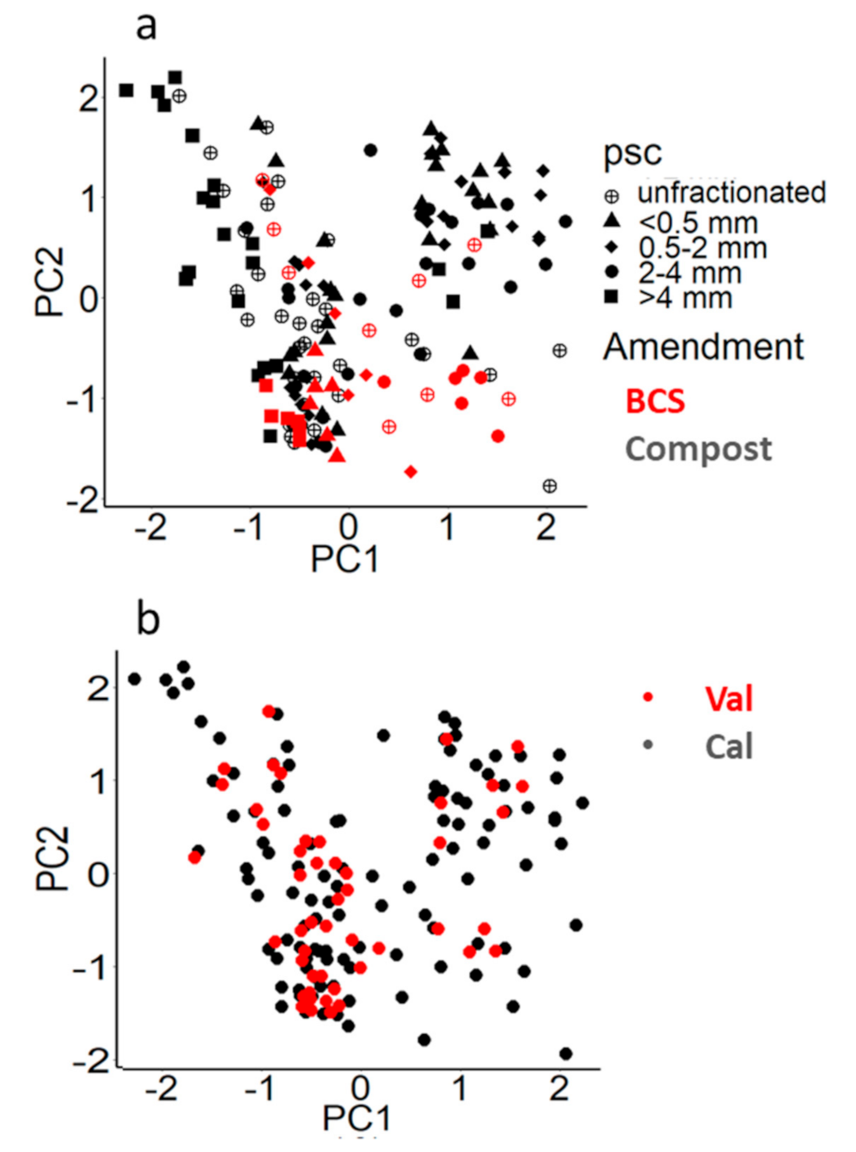
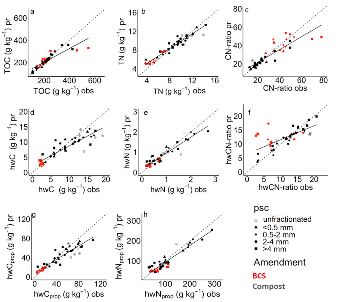
3.3. Calibration of pMIRS SVM Prediction Models for Particle Size Classes of OA

The principal component analysis of MSC corrected pMIRS spectra revealed no clear clusters neither for psc’s nor for OA (Figure 6a), revealing sample set heterogeneity and therefore its suitability for subsequent modeling. Therefore, the k-means sampling partitioning into calibration and validation sample sets showed an even distribution within the PC space (Figure 6b).

In agricultural practice, particle size fractionation prior to OA application would not be convenient for labor and time reasons. Here, it was considered necessary to understand the chemical and physical composition of the varying OA in more detail. Further, the importance of a wide range of target values to be modelled is evident [48]. By creating psc’s, the range of target values was increased in order to potentially strengthen the modelling performance. For pMIRS evaluation of unfractionated OA in combination with size classified samples of the same materials, non-linear SVM regression was of special interest. For a linear approach, e.g., plsr, the samples could not have been considered as independent because spectral information within one size class would possibly occur in unfractionated samples of the same OA. Further, chemical properties and thus spectral information varied among the tested OA and psc’s (Figure 6a), underlining the necessity of a non-linear modelling approach with high generalization potential such as SVM. Support vector machines generally cope with such restrictions in the dataset [30]. Accordingly, the models calibrated via repeated 10-fold cross validation provided excellent correlation with R²_CV values ranging between 0.93 (TOC) and 0.98 (hwC and hwN) and small RMSE_CV for all parameters under study (

Table 4. Calibration (n = 114) and validation (n = 48) parameters and kernel function hyperparameters gamma (γ) and cost (C) of SVM models for the prediction of compost and BCS and associated psc’s via portable MIRS (pMIRS) (CV = cross validation, calibration; pr = prediction, test set validation).

Property	Spectra Pre-Treatment	RMSE		R2		RPIQ		γ	C
		CV	pr	CV	pr	CV	pr
TOC (g kg−1)	1st der	18.8	44.7	0.93	0.77	4.34	1.19	0.5	50
TN (g kg−1)	MSC	0.7	0.9	0.94	0.93	4.80	5.70	0.1	10
CN-ratio	1st der + SG	3.44	7.00	0.94	0.79	2.99	2.72	0.5	100
hwC (g kg−1)	1st der + SG	0.65	2.55	0.98	0.81	10.09	3.87	1	25
hwN (g kg−1)	MSC	0.09	0.22	0.98	0.89	9.37	3.33	0.5	10
hwCN-ratio	SNV	0.10	3.65	0.97	0.49	8.54	2.03	0.1	50
hwCprop (g kg−1)	1st der + SG	4.6	12.8	0.96	0.85	7.33	4.07	1	10
hwNprop (g kg−1)	MSC	1.0	21.1	0.96	0.88	7.98	2.20	0.5	100

). For test set validations, SVM provided good to excellent predictive accuracies and model robustness for TOC, TN, CN-ratio, hwN, hwN_prop, hwC, and hwC_prop. These test set results are in line with [49], who found best validation accuracies for a SVM approach predicting SOC and TN, although via near infrared spectroscopy.

Best model validations were obtained for N pools with highest R²_pr values ranging from 0.88 (hwN_prop) to 0.93 (TN), and low prediction errors and RPIQ_pr values ranging from 2.2 to 5.7, showing excellent model robustness. Test set validation for hwC and hwN showed good model robustness and correlation of predicted and observed laboratory values with RPIQ_pr values of 3.87 and 3.33 and R²_pr values of 0.81 and 0.89, respectively. These results suggest a good suitability of the SVM approach for the above-described C and N parameters. Findings of other authors [29,42] who used and compared SVM with linear methods for MIRS modelling generally support these results, although they were not obtained for organic materials but for soil samples with far smaller C and N contents.

In BCS, most parameters under study revealed rather small variations as compared to composts (Figure 3). Nevertheless, hwC and hwN values and variations of BCS were correctly predicted by the SVM models (Figure 7d,e), which, however, were calibrated upon BCS and composts together. Further, test set values of hwC_prop and hwN_prop were predicted with high accuracy (Figure 7g,h). However, accuracies of SVM models obtained for the test set validation of the hwCN-ratio were not satisfactory, although CV results suggested excellent model statistics (Table 4). From Figure 7f, it is visible that this was mostly caused by false predictions of larger psc’s (2–4 mm and >4 mm) for BCS. Although test set validation accuracies for TOC (R²_pr = 0.77) and CN-ratio (R²_pr: 0.79) were better compared to hwCN-ratio (R²_pr = 0.49), the same trend of misclassified parameters for these psc’s can be observed (Figure 7a,c). For these C pools, the psc > 4 mm revealed the highest variation for both OA (see Section 3.1, Figure 3). A wide range of target values is generally regarded beneficial for model robustness [48]. However, high variation of chemical compounds affiliated to the examined parameters may lead to lower model performance because non-similarity of calibration and validation samples greatly influences the obtained results [50]. Even though SVM are considered to have good generalization capacity [30], our results suggest that varying OA origin and, consequently, differing chemical composition diminished model robustness and therefore test set validation. Further, the calibration dataset contained fewer BCS than compost samples, which probably affected validation accuracy for properties of BCS samples.

As the hw-pool characterizes labile C and N fractions, its proportion of the total C and N concentrations is an important indicator for potential C storage after application in cultivated soils. Therefore, the direct prediction of hwC_prop and hwN_prop of pMIRS spectra for a broad range of OA is a step towards a fast determination of labile C fractions before soil incorporation. Results showed good model validation accuracy (Figure 7g,h) and excellent to good model robustness (hwC_prop RPIQ_pr = 4.07; hwN_prop RPIQ_pr = 2.2) for both parameters. All in all, pMIRS in combination with this SVM modelling approach was shown to be a convenient method for the quick determination of OA properties related to expected C storage potential for a broad range of OA.

4. Conclusions

The chosen C and N parameters can be considered as convenient indicators before soil incorporation for a potential C storage of OA. The large variation of chemical and physical properties of the selected organic amendments and their psc’s was underlined by the laboratory analyses and revealed the necessity of a rapid determination method to characterize these materials. As portable MIRS instruments recently became available, the implementation of these instruments towards routine applications became necessary. In this study, models calibrated on pMIRS spectra were equivalent or superior to those from bMIRS. Yet, both instruments provided robust and accurate performance for most parameters under study. Support vector machines are a crucial part of the procedure because large variation, auto-correlation, and non-linearity of target parameters do not allow linear calibrations. To further develop the implementation of pMIRS devices for evaluating potential C storage of OA in management of cultivated soils, further research should focus on (i) the development of reduced sample preparation to cope with surface roughness for on-site measurements and (ii) test the non-linear SVM approach on a more diverse dataset that includes a wider range of composts, especially BCS products, to enhance model robustness for unknown samples. Further, for specific information on important spectral regions for SVM model calibrations and to gain further insights for future work, research could combine a spectral variable importance approach with SVM calibrations.

References

1. Gregory, A.S.; Ritz, K.; McGrath, S.P.; Quinton, J.N.; Goulding, K.W.T.; Jones, R.J.A.; Harris, J.A.; Bol, R.; Wallace, P.; Pilgrim, E.S.; et al. A review of the impacts of degradation threats on soil properties in the UK. Soil Use Manag. 2015, 31, 1–15. [Google Scholar] [CrossRef] [PubMed] [Green Version]
2. Kammann, C.I.; Schmidt, H.-P.; Messerschmidt, N.; Linsel, S.; Steffens, D.; Müller, C.; Koyro, H.-W.; Conte, P.; Joseph, S.; Stephen, J. Plant growth improvement mediated by nitrate capture in co-composted biochar. Sci. Rep. 2015, 5, 11080. [Google Scholar] [CrossRef]
3. Atkinson, C.J. How good is the evidence that soil-applied biochar improves water-holding capacity? Soil Use Manag. 2018, 34, 177–186. [Google Scholar] [CrossRef] [Green Version]
4. Saidy, A.R.; Smernik, R.J.; Baldock, J.A.; Kaiser, K.; Sanderman, J. The sorption of organic carbon onto differing clay minerals in the presence and absence of hydrous iron oxide. Geoderma 2013, 209–210, 15–21. [Google Scholar] [CrossRef]
5. Lal, R. Soil carbon sequestration impacts on global climate change and food security. Science 2004, 304, 1623–1627. [Google Scholar] [CrossRef] [Green Version]
6. Brenzinger, K.; Drost, S.M.; Korthals, G.; Bodelier, P.L.E. Organic Residue Amendments to Modulate Greenhouse Gas Emissions From Agricultural Soils. Front. Microbiol. 2018, 9, 3035. [Google Scholar] [CrossRef] [PubMed] [Green Version]
7. Thangarajan, R.; Bolan, N.S.; Tian, G.; Naidu, R.; Kunhikrishnan, A. Role of organic amendment application on greenhouse gas emission from soil. Sci. Total Environ. 2013, 465, 72–96. [Google Scholar] [CrossRef]
8. Wang, H.; Ren, T.; Yang, H.; Feng, Y.; Feng, H.; Liu, G.; Yin, Q.; Shi, H. Research and Application of Biochar in Soil CO2 Emission, Fertility, and Microorganisms: A Sustainable Solution to Solve China’s Agricultural Straw Burning Problem. Sustainability 2020, 12, 1922. [Google Scholar] [CrossRef] [Green Version]
9. Ding, Y.; Liu, Y.; Liu, S.; Li, Z.; Tan, X.; Huang, X.; Zeng, G.; Zhou, L.; Zheng, B. Biochar to improve soil fertility. A review. Agron. Sustain. Dev. 2016, 36. [Google Scholar] [CrossRef] [Green Version]
10. Wang, Y.; Villamil, M.B.; Davidson, P.C.; Akdeniz, N. A quantitative understanding of the role of co-composted biochar in plant growth using meta-analysis. Sci. Total Environ. 2019, 685, 741–752. [Google Scholar] [CrossRef] [PubMed]
11. Lehmann, J.; Joseph, S. (Eds.) Biochar for Environmental Management: Science, Technology and Implementation, 2nd ed.; Routledge, Taylor & Francis Group: London, UK; New York, NY, USA, 2015; ISBN 9780415704151. [Google Scholar]
12. Lata Verma, S.; Marschner, P. Compost effects on microbial biomass and soil P pools as affected by particle size and soil properties. J. Soil Sci. Plant Nutr. 2013. [Google Scholar] [CrossRef] [Green Version]
13. Körschens, M.; Weigel, A.; Schulz, E. Turnover of soil organic matter (SOM) and long-term balances-tools for evaluating sustainable productivity of soils. Z. Pflanzenernaehr. Bodenk. 1998, 161, 409–424. [Google Scholar] [CrossRef]
14. Mohanty, M.; Sinha, N.K.; Sammi Reddy, K.; Chaudhary, R.S.; Subba Rao, A.; Dalal, R.C.; Menzies, N.W. How Important is the Quality of Organic Amendments in Relation to Mineral N Availability in Soils? Agric. Res. 2013, 2, 99–110. [Google Scholar] [CrossRef]
15. Körschens, M. Der organische Kohlenstoff im Boden (C org )-Bedeutung, Bestimmung, Bewertung Soil organic carbon (Corg)–importance, determination, evaluation. Arch. Agron. Soil Sci. 2010, 56, 375–392. [Google Scholar] [CrossRef]
16. Ghani, A.; Dexter, M.; Perrott, K. Hot-water extractable carbon in soils: A sensitive measurement for determining impacts of fertilisation, grazing and cultivation. Soil Biol. Biochem. 2003, 35, 1231–1243. [Google Scholar] [CrossRef]
17. Zmora-Nahum, S.; Markovitch, O.; Tarchitzky, J.; Chen, Y. Dissolved organic carbon (DOC) as a parameter of compost maturity. Soil Biol. Biochem. 2005, 37, 2109–2116. [Google Scholar] [CrossRef]
18. Ros, G.H.; Hoffland, E.; van Kessel, C.; Temminghoff, E.J. Extractable and dissolved soil organic nitrogen–A quantitative assessment. Soil Biol. Biochem. 2009, 41, 1029–1039. [Google Scholar] [CrossRef]
19. Zhou, X.; Chen, C.; Wu, H.; Xu, Z. Dynamics of soil extractable carbon and nitrogen under different cover crop residues. J. Soils Sediments 2012, 12, 844–853. [Google Scholar] [CrossRef]
20. Pätzold, S.; Leenen, M.; Frizen, P.; Heggemann, T.; Wagner, P.; Rodionov, A. Predicting plant available phosphorus using infrared spectroscopy with consideration for future mobile sensing applications in precision farming. Precis. Agric. 2020, 21, 737–761. [Google Scholar] [CrossRef] [Green Version]
21. Leenen, M.; Welp, G.; Gebbers, R.; Pätzold, S. Rapid determination of lime requirement by mid-infrared spectroscopy: A promising approach for precision agriculture. J. Plant Nutr. Soil Sci. 2019, 182, 953–963. [Google Scholar] [CrossRef] [Green Version]
22. Bornemann, L.; Welp, G.; Amelung, W. Particulate Organic Matter at the Field Scale: Rapid Acquisition Using Mid-Infrared Spectroscopy. Soil Sci. Soc. Am. J. 2010, 74, 1147–1156. [Google Scholar] [CrossRef]
23. Viscarra Rossel, R.A.; Walvoort, D.; McBratney, A.B.; Janik, L.J.; Skjemstad, J.O. Visible, near infrared, mid infrared or combined diffuse reflectance spectroscopy for simultaneous assessment of various soil properties. Geoderma 2006, 131, 59–75. [Google Scholar] [CrossRef]
24. Hutengs, C.; Ludwig, B.; Jung, A.; Eisele, A.; Vohland, M. Comparison of Portable and Bench-Top Spectrometers for Mid-Infrared Diffuse Reflectance Measurements of Soils. Sensors 2018, 18, 993. [Google Scholar] [CrossRef] [PubMed] [Green Version]
25. Hutengs, C.; Seidel, M.; Oertel, F.; Ludwig, B.; Vohland, M. In situ and laboratory soil spectroscopy with portable visible-to-near-infrared and mid-infrared instruments for the assessment of organic carbon in soils. Geoderma 2019, 355, 113900. [Google Scholar] [CrossRef]
26. Dhawale, N.M.; Adamchuk, V.I.; Prasher, S.O.; Viscarra Rossel, R.A.; Ismail, A.A.; Kaur, J. Proximal soil sensing of soil texture and organic matter with a prototype portable mid-infrared spectrometer. Eur. J. Soil Sci. 2015, 66, 661–669. [Google Scholar] [CrossRef]
27. Sisouane, M.; Cascant, M.M.; Tahiri, S.; Garrigues, S.; El Krati, M.; Boutchich, G.E.K.; Cervera, M.L.; de La Guardia, M. Prediction of organic carbon and total nitrogen contents in organic wastes and their composts by Infrared spectroscopy and partial least square regression. Talanta 2017, 167, 352–358. [Google Scholar] [CrossRef] [PubMed]
28. Meissl, K.; Smidt, E.; Schwanninger, M.; Tintner, J. Determination of humic acids content in composts by means of near- and mid-infrared spectroscopy and partial least squares regression models. Appl. Spectrosc. 2008, 62, 873–880. [Google Scholar] [CrossRef]
29. Deiss, L.; Margenot, A.J.; Culman, S.W.; Demyan, M.S. Tuning support vector machines regression models improves prediction accuracy of soil properties in MIR spectroscopy. Geoderma 2020, 365, 114227. [Google Scholar] [CrossRef]
30. Mountrakis, G.; Im, J.; Ogole, C. Support vector machines in remote sensing: A review. ISPRS J. Photogramm. Remote Sens. 2011, 66, 247–259. [Google Scholar] [CrossRef]
31. Cortes, C.; Vapnik, V. Support-Vector Networks. Mach. Learn. 1995, 20, 273–297. [Google Scholar] [CrossRef]
32. Ivanciuc, O. Applications of Support Vector Machines in Chemistry. In Reviews in Computational Chemistry; Lipkowitz, K.B., Ed.; Wiley: Chichester, UK, 2007; pp. 291–400. ISBN 9780470116449. [Google Scholar]
33. Mantero, P.; Moser, G.; Serpico, S.B. Partially Supervised classification of remote sensing images through SVM-based probability density estimation. IEEE Trans. Geosci. Remote Sens. 2005, 43, 559–570. [Google Scholar] [CrossRef]
34. Acevedo, F.J.; Jiménez, J.; Maldonado, S.; Domínguez, E.; Narváez, A. Classification of wines produced in specific regions by UV-visible spectroscopy combined with support vector machines. J. Agric. Food Chem. 2007, 55, 6842–6849. [Google Scholar] [CrossRef] [PubMed]
35. Meyer, D.; Dimitriadou, E.; Hornik, K.; Weingassel, A.; Leich, F.; Chang, C.-C.; Lin, C.-C. R package e1071: Misc Functions of the Departemt of Statistics, Probability Thery Group, TU Wien: Version 1.7-4 2020. Available online: https://cran.r-project.org/web/packages/e1071/index.html (accessed on 29 March 2021).
36. Stevens, A.; Ramirez-Lopez, L.; Hans, G. R Package Prospectr: Miscellaneous Functions for Processing and Sample Selection of Spectroscopic Data: Version 0.2.1 2020. Available online: https://cran.r-project.org/web/packages/prospectr/index.html (accessed on 29 March 2021).
37. Wickham, H.; Chang, W.; Henry, L.; Pedersen, T.L.; Takahashi, K.; Wilke, C.; Woo, K.; Yutani, H.; Dunnington, D. R Package ggplot2: Create Elegant Data Visualisations Using the Grammar of Graphics: Version 3.3.3 2020. Available online: https://cran.r-project.org/web/packages/ggplot2/index.html (accessed on 29 March 2021).
38. Stevens, A.; Ramirez-Lopez, L. An Introduction to the Prospectr Package. R Package Vignette, Report No.: R Package Version 0.1, 3. 2014. Available online: https://cran.r-project.org/web/packages/prospectr/vignettes/prospectr.html (accessed on 29 March 2021).
39. Scholkopf, B.; Smola, A.J.; Williamson, R.C.; Bartlett, P.L. New support vector algorithms. Neural Comput. 2000, 12, 1207–1245. [Google Scholar] [CrossRef] [PubMed]
40. Bennett, K.P.; Campbell, C. Support vector machines. SIGKDD Explor. Newsl. 2000, 2, 1–13. [Google Scholar] [CrossRef]
41. Bellon-Maurel, V.; Fernandez-Ahumada, E.; Palagos, B.; Roger, J.-M.; McBratney, A. Critical review of chemometric indicators commonly used for assessing the quality of the prediction of soil attributes by NIR spectroscopy. TrAC Trends Anal. Chem. 2010, 29, 1073–1081. [Google Scholar] [CrossRef]
42. Ludwig, B.; Murugan, R.; Parama, V.R.R.; Vohland, M. Accuracy of Estimating Soil Properties with Mid-Infrared Spectroscopy: Implications of Different Chemometric Approaches and Software Packages Related to Calibration Sample Size. Soil Sci. Soc. Am. J. 2019, 83, 1542–1552. [Google Scholar] [CrossRef] [Green Version]
43. Bongiorno, G.; Bünemann, E.K.; Oguejiofor, C.U.; Meier, J.; Gort, G.; Comans, R.; Mäder, P.; Brussaard, L.; de Goede, R. Sensitivity of labile carbon fractions to tillage and organic matter management and their potential as comprehensive soil quality indicators across pedoclimatic conditions in Europe. Ecol. Indic. 2019, 99, 38–50. [Google Scholar] [CrossRef]
44. Fischer, D.; Glaser, B. Synergisms between Compost and Biochar for Sustainable Soil Amelioration. In The Waste Oil Resulting from Crude Oil Microbial Biodegradation in Soil; Zyakun, A.M., Boronin, A.M., Kochetkov, V.V., Eds.; INTECH Open Access Publisher: London, UK, 2012; ISBN 978-953-307-925-7. [Google Scholar]
45. Stumpe, B.; Weihermüller, L.; Marschner, B. Sample preparation and selection for qualitative and quantitative analyses of soil organic carbon with mid-infrared reflectance spectroscopy. Eur. J. Soil Sci. 2011, 62, 849–862. [Google Scholar] [CrossRef]
46. Soriano-Disla, J.M.; Janik, L.J.; Allen, D.J.; McLaughlin, M.J. Evaluation of the performance of portable visible-infrared instruments for the prediction of soil properties. Biosyst. Eng. 2017, 161, 24–36. [Google Scholar] [CrossRef]
47. Jia, X.; Chen, S.; Yang, Y.; Zhou, L.; Yu, W.; Shi, Z. Organic carbon prediction in soil cores using VNIR and MIR techniques in an alpine landscape. Sci. Rep. 2017, 7, 2144. [Google Scholar] [CrossRef] [Green Version]
48. Cécillon, L.; Barthès, B.G.; Gomez, C.; Ertlen, D.; Genot, V.; Hedde, M.; Stevens, A.; Brun, J.J. Assessment and monitoring of soil quality using near-infrared reflectance spectroscopy (NIRS). Eur. J. Soil Sci. 2009, 60, 770–784. [Google Scholar] [CrossRef] [Green Version]
49. Ludwig, B.; Murugan, R.; Parama, V.R.R.; Vohland, M. Use of different chemometric approaches for an estimation of soil properties at field scale with near infrared spectroscopy. J. Plant Nutr. Soil Sci. 2018, 181, 704–713. [Google Scholar] [CrossRef]
50. Bellon-Maurel, V.; McBratney, A. Near-infrared (NIR) and mid-infrared (MIR) spectroscopic techniques for assessing the amount of carbon stock in soils–Critical review and research perspectives. Soil Biol. Biochem. 2011, 43, 1398–1410. [Google Scholar] [CrossRef]
Figure 1. Mid-infrared spectrometers (MIRS) used for spectra acquisition (a) benchtop MIRS Bruker Tensor 27 (b) portable MIRS Agilent 4300.
Agronomy 11 00659 g001
Figure 2. Conventionally analyzed properties of unfractionated compost and BCS samples (n = 45) of (a) total organic carbon (TOC), (b) total nitrogen (TN), (c) ratio of TOC to TN (CN-ratio), (d) hot-water extractable carbon (hwC), (e) hot-water extractable nitrogen (hwN), (f) ratio of hwC to hwN (hwCN-ratio), (g) proportion of hwC to TOC (hwCprop), (h) proportion of hwN to TN (hwNprop).
Agronomy 11 00659 g002
Figure 3. Conventionally analyzed samples of different organic amendments (OA) particle size classes (psc) (n = 117) for (a) TOC, (b) TN, (c) CN-ratio, (d) hwC, (e) hwN, (f) hwCN-ratio, (g) proportion of hwC to TOC (hwCprop), (h) proportion of hwN to TN (hwNprop).
Agronomy 11 00659 g003
Figure 4. Principal components (PC1 and PC2 scores) of multiplicative scatter correction (MSC)-corrected calibration (black; n = 31) and validation (red; n = 14) samples as selected by k-means sampling and associated MIRS spectra (a,b) benchtop MIRS and (c,d) portable MIRS.
Agronomy 11 00659 g004
Figure 5. Test set validation: support vector machines (SVM) predicted (pr) and observed (obs) (n = 14) values of benchtop and portable MIRS spectra for (a) TOC, (b) TN, (c) CN-ratio, (d) hwC, (e) hwN, (f) hw-CN-ratio, (g) proportion of hwC to TOC (hwCprop), (h) proportion of hwN to TN (hwNprop).
Agronomy 11 00659 g005
Figure 6. (a) PC1 and PC2 scores of OA samples and particle size classes (psc’s) and (b) PC1 and PC2 scores of OA calibration (black) and validation (red) samples (BCS and compost).
Agronomy 11 00659 g006
Figure 7. Test set validation SVM predicted (pr) and observed (obs) for (a) TOC, (b) TN, (c) CN-ratio, (d) hwC, (e) hwN, (f) hw-CN-ratio, (g) proportion of hwC to TOC (hwCprop), and (h) proportion of hwN to TN (hwNprop) in different OA size classes (pMIRS test set, n = 48).
Agronomy 11 00659 g007