A Practical Application of Unsupervised Machine Learning for Analyzing Plant Image Data Collected Using Unmanned Aircraft Systems

Abstract

Unmanned aircraft systems are increasingly used in data-gathering operations for precision agriculture, with compounding benefits. Analytical processing of image data remains a limitation for applications. We implement an unsupervised machine learning technique to efficiently analyze aerial image data, resulting in a robust method for estimating plant phenotypes. We test this implementation in three settings: rice fields, a plant nursery, and row crops of grain sorghum and soybeans. We find that unsupervised subpopulation description facilitates accurate plant phenotype estimation without requiring supervised classification approaches such as construction of reference data subsets using geographic positioning systems. Specifically, we apply finite mixture modeling to discern component probability distributions within mixtures, where components correspond to spatial references (for example, the ground) and measurement targets (plants). Major benefits of this approach are its robustness against ground elevational variations at either large or small scale and its proficiency in efficiently returning estimates without requiring in-field operations other than the vehicle overflight. Applications in plant pathosystems where metrics of interest are spectral instead of spatial are a promising future direction.

1. Introduction

Unmanned aircraft systems (UASs) have been discussed as a cornerstone of precision agriculture [1,2,3,4,5,6], supporting the collection of timely and abundant data at expansive spatial scales through low-altitude remote sensing (LARS). Data collected through LARS are of high resolution and volume and can easily represent spatial scales exceeding the size of current agricultural operations [7,8]. UAS image collection can be utilized when other means would be logistically limited, for example in flooded-field systems such as rice. Thermal and other spectral data can be collected at increasingly high resolution and detail as imaging technology advances [9,10,11,12,13,14,15]. As beyond-line-of-sight applications become feasible, the potential spatial scale of data collected through LARS becomes practically unlimited. The advancement of LARS applications also makes them useful where financial or logistical resources are limited, providing information with a short turnaround time and low cost for small farms or operations in developing countries [2].

Research concerning LARS is increasing, and work is ongoing to translate this research to applications in commercial agriculture [15,16,17,18]. LARS techniques have been used to describe various plant metrics in fields, notably plant height as a phenotype itself [19,20,21,22], and surrogate metrics of economic interest such as yield [7,22,23,24,25]. Using UASs, plant height has been studied as a readily measurable response to the uptake of nutrients such as phosphorus [23] and nitrogen [24,25,26,27]. Additional applications of LARS include weed identification and mapping in fields [28,29], characterizing tree canopies [30], observing tree recovery after pruning [17], and the detection of disease outbreaks [13,31]. As LARS technology improves, sophisticated applications of well-established findings are enabled—for example, in 1991, a demonstration established that multispectral measurement could be used to predict aspects of rust severity [32], and since then, applications have advanced commensurate with technology and researchers developing new analytical techniques [15,33,34].

Utilization of LARS also faces challenges, especially in the setting of commercial agriculture where users of the technology seek to implement LARS in response to a current need, instead of for the purpose of advancing the underlying technology [1,4]. A major limitation to the practical use of LARS for crop phenotyping is the efficiency of the application of the technology [1,4,5,6], such that there is need to streamline data analysis for practical use. Though the economic feasibility of LARS approaches for producers is often implied by referring to on-vehicle sensors as “consumer grade,” several analysis steps between image acquisition and result generation are intensive and expensive. A non-trivial problem related to physical characterization of crops is the requirement to have a positional reference for measurement. On-vehicle sensors are photonic in nature and principally record the wavelength and intensity of emissions. A global positioning system (GPS) receiver on a vehicle provides the ability to record the position of a photonic sensor—the three-dimensional orientation of which may also be recorded by accelerometry. Together, photography and positional data can be used by a structure-from-motion algorithm to infer three-dimensional structure from two-dimensional images [35]. In common situations where LARS is used to provide physical characterization of a crop, for example the average height of above-ground biomass, there is a requirement for the position of the ground to be known and used for reference [16,23]. Approaches to this include equipment- and software-intensive construction of a reference surface using GPS “control points,” or the explicit classification (computer automated or by eye) of plants vs. background for comparison [7,8,36]. GPS control points constitute references that are of known geospatial position, and also image-recorded position, so that the two can be reconciled in analytical processing [7,8,10,16,21,36]. The points are effectively anchors for processing algorithms to use in constructing a geospatially explicit rendition of physical objects from imagery. The technique is not without merit, and not without cost.

Here, we focus on addressing these challenges using only image data, without GPS control points for ground surface construction, and without computer vision for image classification or feature extraction. We test the utility of an unsupervised machine learning technique (hereafter “unsupervised learning”) for advancing the analytical use of UAS data acquired by UAS-based LARS, intending to complement improvements in data quality currently being made through engineering. We believe that advancements in the analytical use of data will support optimization of future data collection and interpretation. Attempting to advance the utility of LARS in general, we use data from different agricultural settings and from different LARS platforms. We explore ways of presenting results and the underlying analytical methods of their generation and discuss how each may be optimized to better serve producers’ purposes.

2. Materials and Methods

2.1. Sites, Materials and Data

A field trial of nitrogen fertilizer application rates and timing for rice (Oryza sativa L.) crops was conducted in 2017 at the Texas A&M AgriLife Research Center in Beaumont, TX, USA. The project investigated the inbred cultivar Clearfield 272 (Horizon Ag, Memphis, TN, USA), and the hybrid XP753 (RiceTec Inc., Alvin, TX, USA). Rice was drill-planted on May 16 and grown with flush irrigation until the four- to five-leaf growth stage, after which a permanent flood (5–10 cm depth) was imposed and maintained until plant maturity. Aerial imagery of rice fields was collected on August 2, 2017 from at 15 m above ground level (AGL). A 245 × 45 m field was divided into six research blocks, each consisting of forty 4.8 × 1.5 m plots wherein ten experimental treatments were each replicated four times. Nitrogen fertilizer (urea) was applied at four time points: pre-planting, pre-flooding, panicle initiation, and late booting (Table S1). All other field operations followed the 2014 Texas Rice Production Guidelines [37].

A private nursery (Amerson’s Nursery) in Lamar, SC, USA, was aerially photographed, including a diversity of plants on May 13, 2018. Flights were flown at 15 m AGL. Our effort in this instance was to collect and process image data on a variety of plants to investigate the performance and robustness of an analytical approach. Areas populated by shrubs, trees, and potted plants were photographed for this purpose.

At the Clemson University Edisto Research and Educational Center (REC) in Blackville, SC, USA, a rotational study concerning agriculturally relevant nematodes was underway in 2018, aerial imagery of fields of soybean (Glycine max L.) and grain sorghum (Sorghum bicolor (L.) Moench) was collected on July 23, 2018. Here, our aim was to test approaches for their ability to recover accurate height estimates validated against “ground truth” measurements taken by personnel in the field. Accordingly, rectangular pieces of white cardboard were placed at ground level in these fields to mark locations at which in-field measurements were made on surrounding plants. Five randomly selected plants were measured with a ruler at each of eight such locations (four for grain sorghum and four for soybean), and these measurements were used for comparison with LARS-based estimates of height.

Supplemental Figures S1–S3 show representative imagery from each location.

2.2. Unmanned Aircraft Systems

The flight platform used was Dà-Jiāng Innovations (DJI) Phantom 4 (Dà-Jiāng Innovations, Shenzhen, China), with an attached red-green-blue (RGB) camera. The flight platform used a 30 mm² CMOS sensor with 12.4 effective megapixels. The viewing angle was 94°, the electronic shutter speeds were 8–1/8000 s, and the image size was 4000 × 3000 pixels. Raw images were stored in digital negative (DNG) format and developed to joint photographic experts group (JPEG) format for analysis. The system used a GPS and global navigation satellite system (GLONASS) for positioning. Images were stored on a micro secure digital (SD) card. Flights were either structured using the flight planning functions of Pix4Dmapper software version 4.1 (Pix4D, Lausanne, Switzerland) [38] or conducted manually. Flights in Texas were planned, involving a double grid pattern with 75% pairwise overlap in both along-track and cross-track directions between sequentially adjacent photographs. Flights in South Carolina were manually directed, involving alternating forward and reverse passes and targeting 80% pairwise overlap between sequentially adjacent photographs in the along-track direction. Degree of overlap was chosen to conform with imaging practices reported in other studies, so that our data acquisition step would be in line with current practices [7,8].

2.3. Image and Data Processing

For each dataset, images were processed using the structure-from-motion algorithm of Pix4Dmapper software, resulting in point clouds. Point clouds comprise points inferred through the algorithm, in which each point is projected onto a three-dimensional space and has a spectral description. The structure-from-motion algorithm uses a single camera to infer three-dimensional structure in the way that multiscopic vision does, but by processing positional variation of the camera through time as equivalent to the physical distance between two or more cameras. Point clouds, as tables, were used directly for analysis. Point clouds were visualized as three-dimensional surface plots (Figure 1) through the G3D procedure (three-dimensional graphics) of the SAS System v9.4 (SAS Institute, Cary, NC, USA) [39] to confirm point cloud processing success, for data subset delineation, and to visually identify potential anomalies or features that could interfere with or be utilized in analysis. Three-dimensional renderings of data involved latitude and longitude for in-field position and height or spectral (red, green, or blue) indices as the third dimension for visualization. Depictions were used to delineate data subsets representing areas of interest—fields, plots, or subplots in the research settings, and areas of the nursery. Random samples of a given size were taken from the dataset for visualization because the resolution of our raw data was much higher than that required for visualizing general features—in other words, we used a reduced-resolution preview of the full-resolution dataset to identify subareas such as plots or field margins, because these areas were easily identifiable without full-resolution depiction. For example, a point cloud representing the rice field at Beaumont, Texas, includes 3.5 million points, and 35 thousand points were randomly selected from the dataset for use in generating visualizations. Full-resolution point clouds were used for analysis.

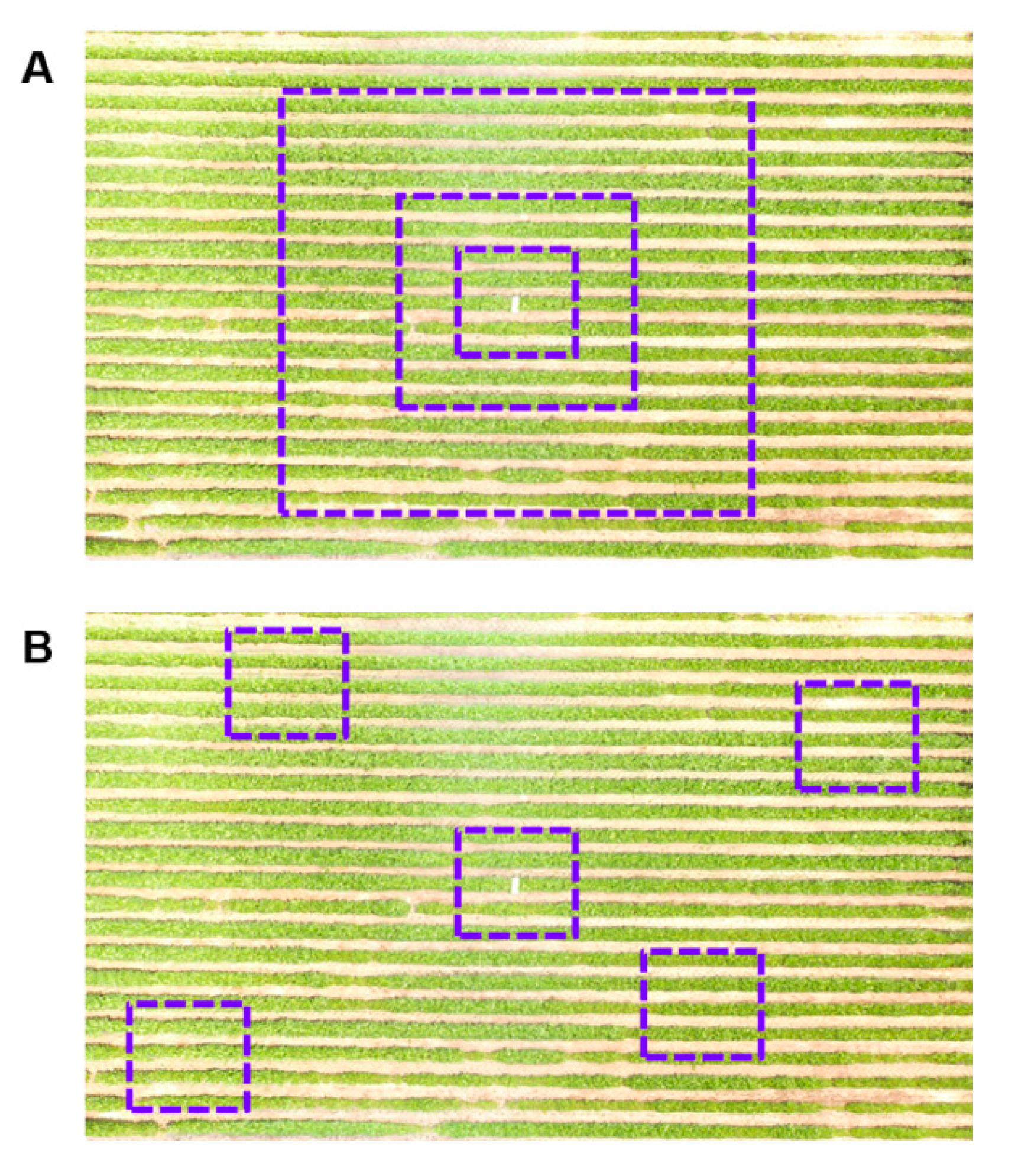
Point clouds were rendered as contour plots using the GCONTOUR procedure of the SAS System v4.3 and visually investigated for quality and representativeness of the depicted area, as compared to images to identify imaged subjects, by eye. Forty plots from the rice research field in Texas were visually identified using a contour map rendered from the point cloud. Treatment information associated with each plot, including timing (date) and amount (kilogram per hectare) of nitrogen addition, was merged with the point cloud dataset by plot for analyzing relationships between treatments and inferred rice plant height. Subsets of point cloud data from Amerson’s Nursery were generated on the basis of plant type, following visual identification of areas targeted for analysis, e.g., an area of potted plants, or an area of a given type of shrub. Subsets of point cloud data from the Edisto REC soybean and grain sorghum fields were generated to investigate how the spatial size of an imaged area can be chosen to optimize the accuracy or precision of estimated plant characteristics: square-shaped sample areas of two, four, eight, sixteen, and thirty-two square meters in area were taken from the whole-field point cloud. Each sample was centered on a reference point indicated by a white piece of cardboard placed at ground level in the field at random. This subsetting was done to emulate a researcher randomly choosing a sample location in a field for inclusion in a dataset.

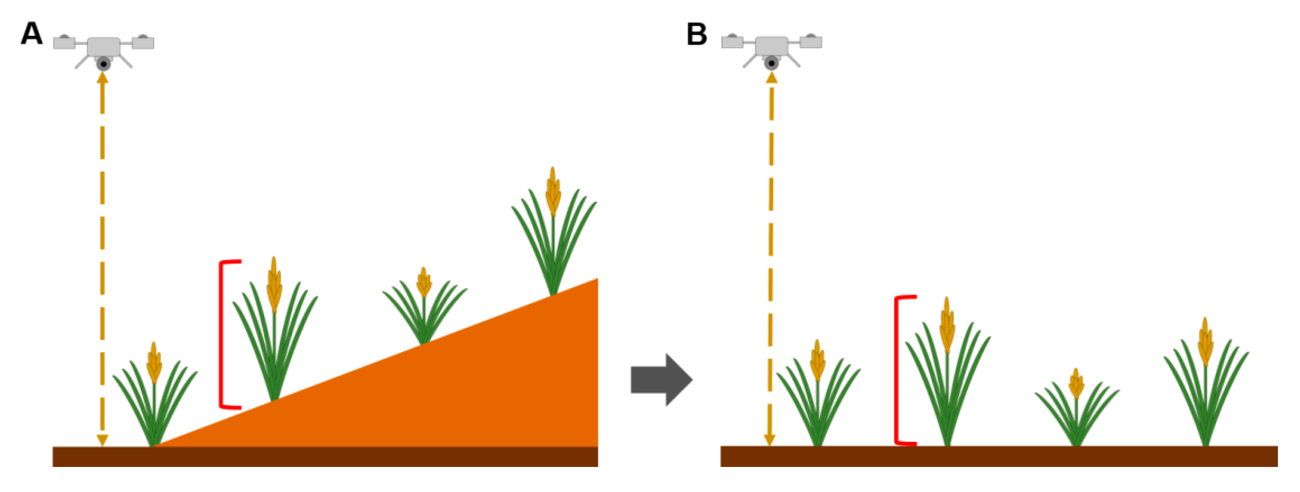
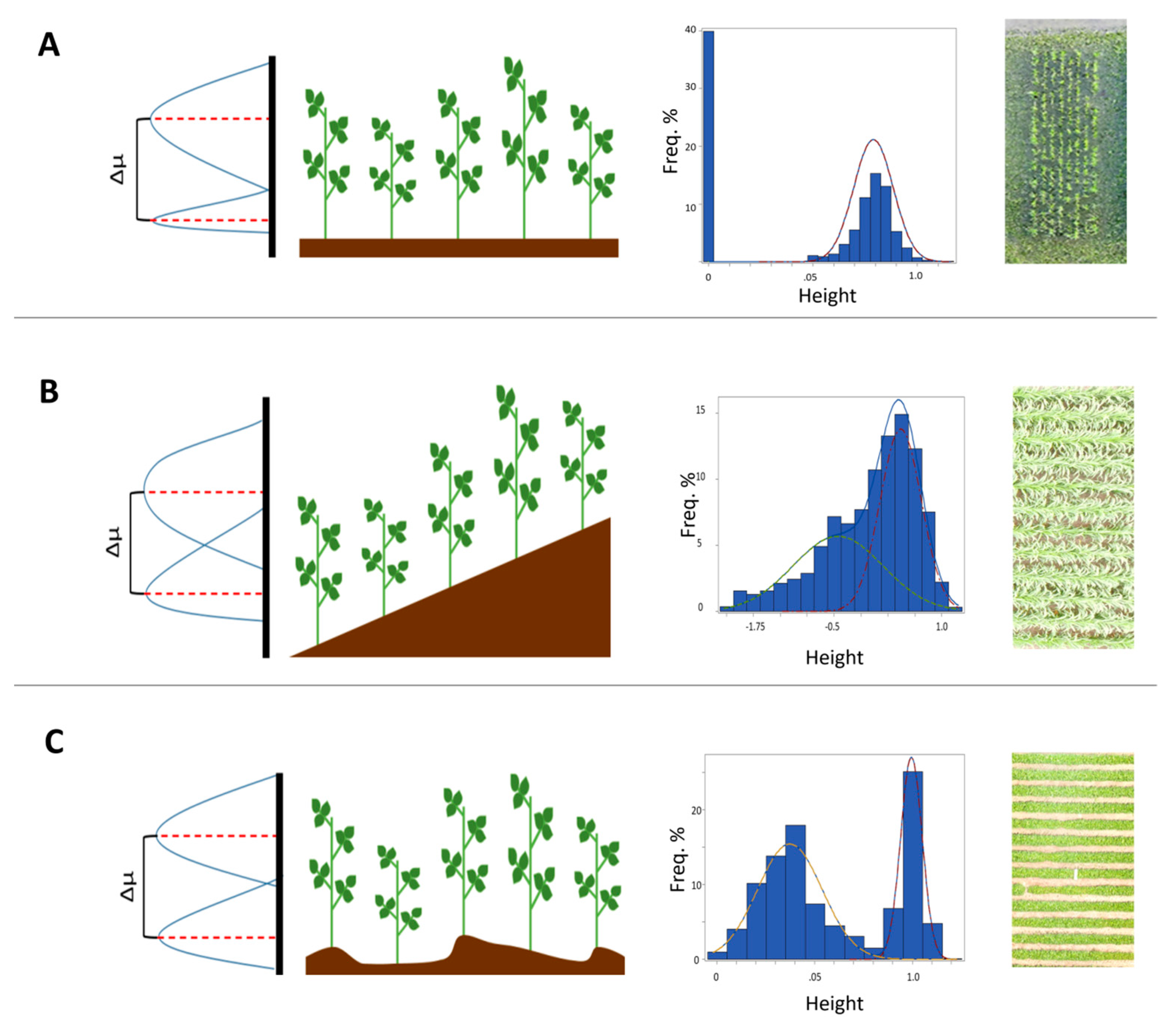
A preliminary finding guided subsequent methods selection. Initial processing of images using Pix4D to generate point clouds resulted in three-dimensional depictions that included artifacts, specifically slopes that are known to not exist in reality, given that the depicted areas are flooded rice fields and thus necessarily level (Figure 2).

The use of GPS control points would result in correcting this issue to a degree proportional to how accurately the points provide for estimating terrain surface. However, in this case, the effect is also easily marginalized by including positional variables (latitude and longitude) as covariates in a generalized linear model of height. For a flat surface (not level, but flat), as was the case for the rice fields, this technique works well. However, for any non-flat surface, terrain variation cannot be described by a linear model without concern that variation in plant height is also being described. The fact that (artifactual) terrain height variation in a special case (rice fields known to be both flat and level) could be marginalized without the use of GPS control points or classification of plants vs. ground suggested that a statistical method could be developed to do this in other cases. We sought a plant height estimation method that would be insensitive to terrain height variation, but without having to describe terrain height variation (as is conventionally done when a digital terrain model is developed). We settled on the unsupervised learning technique of finite mixture modeling, and the following methods were chosen for applying the technique.

2.4. Mixture Modeling

To investigate the applicability and performance of mixture modeling to infer plant height, we fit mixtures of frequency distributions to height observations (points in the cloud), irrespective of pixel class (ground vs. plant), using the finite mixture model (FMM) procedure of the SAS System v9.4. A FMM is a statistical model that describes variation in a population made up of a finite number of subpopulations, without classifying individuals’ subpopulation membership. Equation (1) relates φ, the characteristic function of height, h, varying within a given spatial extent and composed of a number, k, of component Gaussian distributions each, i, with location and dispersion parameters, mean, μ, and variance, σ.

$${\phi }_{\mu ,\sigma }\left(h\right)={\displaystyle \sum }_{i=1}^k{\left(\sqrt{2\pi {\sigma }_i}\right)}^{-1}{e}^{{\left(\frac{-\left(h-{\mu }_i\right)}{2{\sigma }_i}\right)}^2}$$

(1)

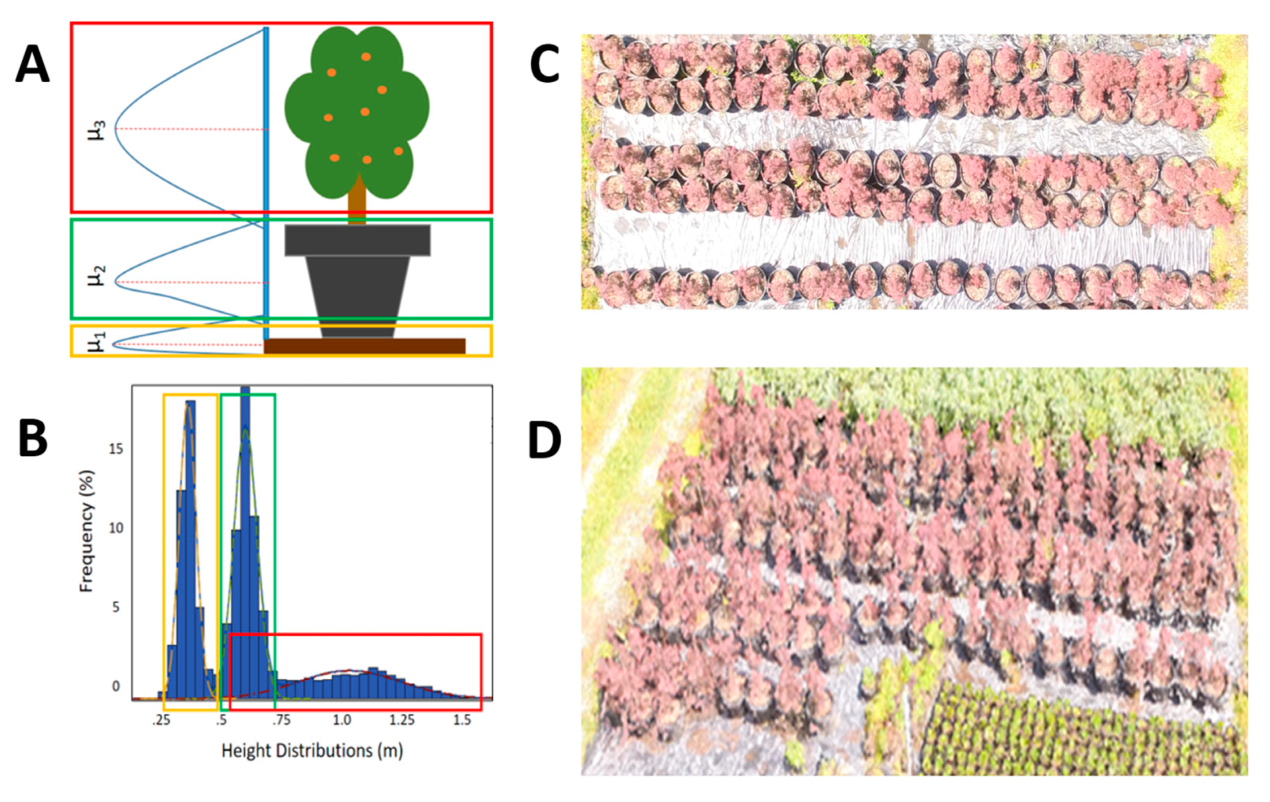
Initially, we compared mixture models with varying numbers of components (k) in order to confirm that k = 2 for images including plant biomass and the ground was an appropriate parameter value. Our expectation was that two subpopulations of points in the cloud would be detectable through this approach: the ground (terrain between plants visible to the UAS), and plant biomass (aboveground plant tissue). In this initial stage, we fit mixture models for k = 1 to k = 5 and confirmed that k = 2 resulted in best fit by minimizing Schwartz’s Bayesian Information Criterion (BIC). In a few instances, the minimum BIC corresponded to k = 3, and visual inspection of histograms of height variation confirmed three distinguishable mixture distribution components. Once we had optimized k for an FMM fit to data from an area of interest, we then proceeded to calculate an average height estimate as the difference between locations (for Gaussian mixture components, μ_i, the means) of “ground” and “plants” distributions. Calculating this difference is possible without needing to classify individual pixels as being members of one or another component distribution. 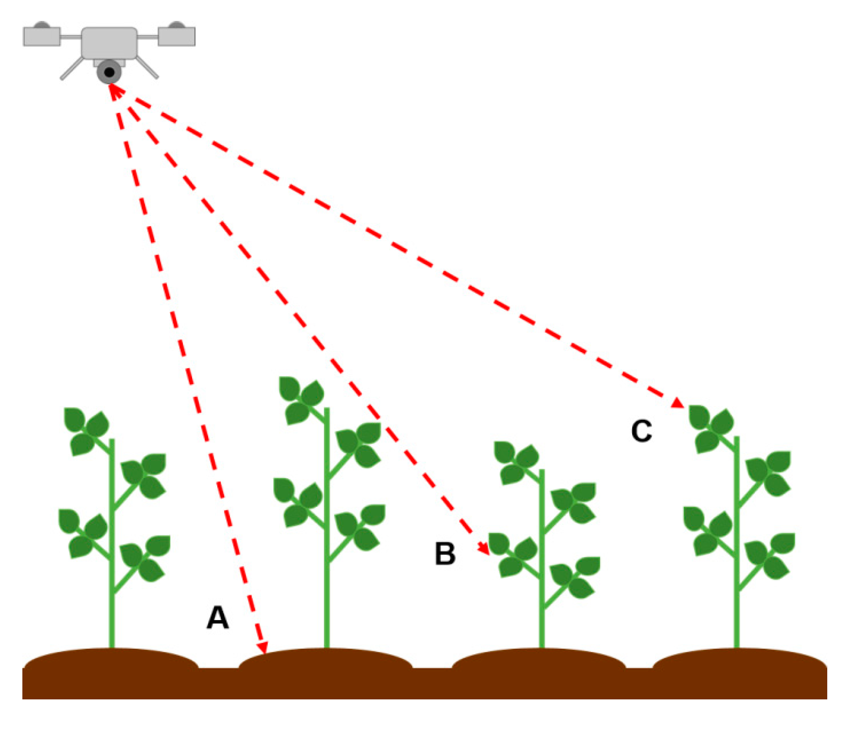For areas in which the optimal value of k was 3, due to some nursery plants being grown in pots, we estimated plant height as the difference between the “pot” and “plants” distributions. Additional comparisons between quantile limits of distribution pairs were calculated, expecting that for important reasons other than average plant height, the distribution of height in a given point cloud should vary. For example, plant row spacing or physical architecture should affect depth of visibility into the canopy (Figure 3) and this can be addressed by referencing different portions of the “plants” distribution.

Where ground-truth data were available (soybean and grain sorghum fields in South Carolina), plant heights were estimated and thereafter tested for validity as predictors of actual measurements, with this validation being conducted through a regression approach using the generalized linear model (GLM) procedure of the SAS System v9.4: actual heights were regressed against predicted heights.

3. Results

3.1. Rice Plant Height and Yield—Beaumont, Texas

A generalized linear model describing rice plant height, including treatment number (as a category), latitude, and longitude as independent variables accounted for 85% of height variation for field N-1, and 87% of height variation for field N-6.

Table 1. Generalized linear model (GLM)-derived and finite mixture model (FMM)-derived height estimates of rice fields N-1 and N-6. The FMM height estimates were given 0.4 m of ground buffer on each side of the rice plots.

Treatment Number	GLM Estimated Height (m)	FMM Estimated Height (m)
Field N-1
1	1.05	1.05
2	0.85	0.84
3	0.79	0.79
4	0.77	0.77
5	0.73	0.73
6	0.97	0.97
7	0.86	0.84
8	0.77	0.77
9	0.74	0.73
10	0.69	0.70
Field N-6
11	0.80	0.80
12	1.21	1.21
13	1.34	1.34
14	1.39	1.39
15	1.36	1.37
16	1.04	1.04
17	1.27	1.32
18	1.31	1.26
19	1.30	1.26
20	1.35	1.35

includes coefficients estimated for this model, which marginalizes artifactual slope that arises from image processing and enhances ability to infer differences arising from treatments applied to plots in a randomized complete block design.

This technique results in a level field, confirmed by observing the slope of “ground” area not occupied by rice plots, which is known to be level due to being flooded with water. Height estimates calculated as the difference between FMM mixture components (“ground” and “plants” distributions) are also shown in Table 1, confirming that in an idealized situation of level and flat ground (obviating the need to construct a digital surface model or use GPS control points), FMM-derived estimates based on the difference between component means are equivalent to estimates calculated by subtracting a fixed ground position from a plot’s average distance from a UAS’s sensor. For FMM-based height estimation, a spatial buffer of 0.4 m was added to each plot to ensure adequate representation of the ground in point cloud data.

3.2. Multiple Plant Species at Amerson’s Nursery—Lamar, SC

Images from Amerson’s Nursery were initially processed, as were those from the rice field at Beaumont, TX, using Pix4D to generate three-dimensional point clouds thereafter analyzed using the FMM procedure of the SAS System. Because the use of FMMs proved well suited to inferring heights of rice plots in the earlier stage of this study, we applied the technique to a variety of plant types to test whether multiple mixture components could be reliably detected across plant types. In this instance FMMs could be used reliably to detect the presence of three mixture components where appropriate (Figure 4), representing ground, pots (being the soil surface contained in a pot), and plants for potted shrubs. Height estimates are generated by calculating the distance between any pair of component means.

3.3. Soybean and Grain Sorghum—Blackville, South Carolina

Images from the Edisto REC at Blackville, SC, were processed as before, first using Pix4D and subsequently analyzing point clouds using SAS.

Reported in

Table 2. Heights estimated from soybean fields using image subsample sizes of four, eight, and sixteen square meters.

FMM Estimated Heights (m)
Area	Field 1	Field 2	Field 3	Field 4
16 m2	0.67	0.69	0.67	0.64
8 m2	0.61	0.67	0.66	0.62
4 m2	0.54	0.65	0.60	0.68
2 m2	0.57	0.66	0.61	0.67

are heights estimated for data subsets corresponding to square areas of four, eight, and sixteen square meters around reference locations indicated by rectangular pieces of white cardboard (Figure 5).

Parameter estimates pertaining to one subfield appear in

Table 3. Representative FMM parameter estimates for a soybean field. μ₁ and μ₂ correspond to the locations of “ground” and “plant” distributions, respectively. σ₁ and σ₂ are respective variances. The difference between μ values is calculated to estimate height, irrespective of the absolute value of μ values. Here, negative height values result due to the global average height being set to zero.

Soybean Field Parameter Estimates
Area (m2)	μ1	μ2	σ1	σ2
32 × 32	−0.382	0.255	0.014	0.026
16 × 16	−0.393	0.228	0.005	0.023
8 × 8	−0.391	0.221	0.003	0.019
4 × 4	−0.391	0.221	0.003	0.019
2 × 2	−0.392	0.268	0.019	0.003

.

These estimated heights were compared with ground measurement to assess the performance of the technique in recovering accurate heights, with the highest correlation being between median point (from point cloud subset) height and ground-truth height (

Table 4. Estimated soybean heights measured in the field. Median estimated values provided maximum description (R² = 0.96) of observed variation.

Estimated Soybean Heights (m)
Field	Ave. Obs.	Fifth	Lower	Mean	Median	Upper	Ninety-Fifth
1	0.49	0.18	0.30	0.59	0.47	0.95	1.05
2	0.53	0.18	0.42	0.62	0.59	1.08	1.20
3	0.47	0.13	0.30	0.71	0.44	1.01	1.10
4	0.44	0.15	0.25	0.83	0.40	0.94	1.02
R2		0.37	0.94	0.71	0.96	0.69	0.81

). When fitting FMMs to data collected from grain sorghum fields with dense canopies, frequently only one mixture component was estimated, preventing calculation of the distance between component means to represent height.

4. Discussion

This study demonstrates the ability of an unsupervised learning technique to robustly generate useful results from LARS data in agricultural settings, with emphasis on efficiency. The approach was to generate three-dimensional point clouds using LARS data collected from different types of agricultural operations and from varying UAS flight patterns, and then to analyze variation without classifying areas or points in the cloud. Implicit in the process of measuring plants for height above ground is differentiation of plants from ground, and many supervised learning analytical approaches address this through classification and subsequent comparison. A conventional approach is to construct the entirety of the “ground” class via linear or other interpolation between GPS control points and treat a spatial subset of point cloud data as the “plants” class. Also common is to construct a surface model from point cloud data, enhancing visualization and summarizing features, but also collapsing variation in a way that prohibits its being analyzed in raw form.

We suggest that a difference between human measurement takers and an aerial sensor can be exploited. Whereas a human on the ground taking a measurement is reliably calibrated (ground position is unlikely to be mistaken), he/she does not record the millions of measurements that are represented in a point cloud assembled from images taken by an aerial sensor. Indeed, the human does not have reason to take millions of measurements because the few taken are likely to be calibrated very accurately. We propose that the aerial imager similarly does not have reason to calibrate relative to ground in the way that the human does because the aerial imager benefits from the generation of a large number of data points. The calibration of measurements derived from aerial imagery can thus be carried out post-measurement, and through a statistical approach. The volume of data thus generated supports unsupervised learning to infer the distance between two components latent in the resultant distribution of heights (Table 2). Results demonstrated that the mean height estimates derived from the FMM are robust to variation in spatial extent being examined (Table 2). Furthermore, the FMM-derived height estimates were well correlated (R² = 0.71) with in-field human-measured soybean heights (Table 3). This process can be generalized to situations in which some background, other than the physical ground, is the reference for comparison. For example, comparisons between colors or temperatures can be made. Such situations include spatial variation in spectral profile arising from disease, stress, or other phenomena of practical interest to agricultural producers. Because the approach does not rely on a priori or computational classification, it negates the consequences of classification error. In an unsupervised learning approach, the difference between plant and ground, or healthy and diseased plants, need only be detectable using analyzed metrics, not defined in terms of what underlies the difference. A producer monitoring a crop for the presence of disease can target areas where two classes of spectral profile are detected for investigation. Because the class-detection result of fitting an FMM does not depend on absolute values, differences between classes can be detected more reliably across varying conditions (lighting, weather, etc.) than may be possible through supervised learning approaches that require reliable classification before analysis. Additionally, FMMs are straightforward to estimate, such that fitting of models for this purpose can be easily accomplished using many statistical analysis platforms.

Application of FMMs to the types of problems faced by agricultural producers is fitting because of how the effort-intensive process of classification is (or is not) conducted. Classification of plant vs. ground in this context is not something that directly informs the agricultural producer—the producer can already readily identify ground vs. plant. Instead, classification is required by algorithms that rely on data being classified for supervised learning activities: these algorithms must know the difference between a “ground” point and a “plant” point before inference may be drawn from comparison between classes. Again, this information is not in itself of use to the producer—the producer does not need to know point or pixel class for any purpose outside of the analytical task being undertaken by the relevant algorithm.

The unsupervised machine learning technique used here provides estimates, but with a reduced number of required steps when compared to other approaches that involve the use of GPS control points and their inclusion in analysis. The presence of multiple classes in a dataset is inferred without data needing to be classified. Thus, we expect the approach taken here can be more efficient, simply on the basis of its requiring fewer activities to execute. An approach that involves GPS control points and supervised classification requires, among other things, (1) construction of physical markers to be detected by computer vision algorithms during orthomosaicking; (2) placement of physical markers in target areas, ensuring visibility to aerial cameras by clearing plant biomass or other materials; (3) precisely georeferencing GPS control points by physically visiting them with GPS equipment; (4) incorporating GPS control points into datasets and constructing terrain maps; (5) subsetting point cloud data to exclude pixels associated with actual terrain, so that statistical characterization of plants can be carried out. There are definitely situations in which these steps are required and advantageous—we highlight the most obvious of these, a situation in which the terrain is not visible to the aerial camera and thus the fitting of FMMs is not possible. However, where these effort-intensive steps are not required, efficiency in phenotyping can be gained by taking an alternative approach that does not require the steps. A consultant or scout operating LARS-based data gathering could collect data in the time it takes to conduct the imaging overflights, process data in the time it takes to assemble a point cloud, and then have an estimate of plant phenotype in the field for discussion with the producer. By fitting FMMs to spatial subsets of data, height estimates can be made precisely despite variable topography of terrain (Figure 6). To construct a model of terrain using GPS control points, those points must be numerous enough to support fitting a terrain model that adequately represents variation in a field. If terrain varies appreciably at small spatial scales, then GPS control points must be distributed densely to account for that variation. However, to compare two latent height classes, those classes need only be each adequately represented by data, and not necessarily identified by class. Height estimates for subareas of a field, sampled randomly or with structure, can be averaged to estimate the overall mean height in a field. As in a Riemann sum, the size of these spatial subsets affects the accuracy of the estimate, practically limited in this case by the minimum size at which mixture distribution components can be reliably differentiated and estimated. We suggest that this approach to LARS data usage combines the well-established practice of random sampling (computing height estimates for multiple data subsets) with the resolution and extent advantages of aerial imagery. Our results demonstrate that small spatial subsets (2 m squares) can be used to generate representative estimates (Table 3).

Additionally, Figure 6 shows how the success of the FMM approach in recovering height estimates means that there is not a need to “level” point clouds or use GPS control points for generating height estimates. Importantly, sources of error or variation that result in a given field not being level can be addressed by the FMM approach regardless of whether those sources are an image-processing artifact, or a real-world sloped or hilly field. Correspondence between GLM- and FMM-derived height estimates (Table 1) confirms that the FMM can implicitly account for terrain variation that is explicitly included as covariates in the GLM. Where this covariate information is unavailable, the FMM approach is more useful. Taken together, these considerations underscore the robustness of the unsupervised learning approach to analyzing image data for practical purposes in agriculture.

Some situations require GPS control points and comparison between a constructed ground and a point cloud of observations. If the ground is not adequately visible to an aerial sensor, the “ground” component of a mixture distribution cannot be estimated. In such situations, calibration for height estimates cannot be accomplished through the technique used here, and a reference surface must be constructed. Thus, the application of this technique is limited to situations in which the ground is visible between crop plants—for example, row crops and early developmental stages of field crops. Situations calling for GPS control points and those well suited to application of FMMs are thus to a degree mutually exclusive. Where plants are dense such that canopy can be reasonably represented by a surface, an FMM attempting to differentiate (obscured) ground from plants will fail to return good estimates, and classification is not likely necessary, because all data in a related point cloud would describe plants. For instance, FMMs fit to data from grain sorghum resulted in only one mixture component, corresponding to the dense canopy of the crop when imaged (Supplemental Figure S4). In this situation, comparison between the plant canopy surface and a ground surface constructed using GPS control points would be required to estimate height. On the other hand, where plants are spaced such that the ground is visible between them and the canopy is discontinuous instead of being like a surface, an FMM is able to address the issue of classification efficiently without having to classify data points (Figure 6). Were explicit classification attempted for comparison of the “plants” points to a constructed ground surface through a supervised learning approach, classification error would result in commensurate phenotype estimate error. In such an approach, excluding generous buffers from analysis to avoid attempting to classify ambiguous data points is not only an additional analysis step with attendant potential for error, but also discards data points that may be informative. Unsupervised learning is more robust in situations to which it is appropriate.

Here, the FMM accounts for overlap between points belonging to each class, without that overlap detrimentally affecting estimates of each class’ mean or other distributional parameters. A threshold-based classification method will misclassify at a rate proportional to the overlap between classes, resulting in biased estimates of class means. This bias will increase as a function of the two components’ difference in proportional contribution to the mixture, and as a function of the difference between the two components’ dispersions. In other words, misclassification is of no consequence to supervised learning-based height estimation if the ground and height classes are equally represented and equally variable in a given dataset. However, as representation and variability differ, misclassification becomes increasingly negative in its impact to such an approach. Again, unsupervised learning accounts for this varying issue more robustly.

5. Conclusions and Future Work

The analytical method described herein was first explored to estimate rice plot height in the absence of GPS control points. An application of the unsupervised machine learning approach, finite mixture modeling, was developed to reliably estimate plant heights in various terrain configurations. Using imagery data from a nursery, we determined that FMMs could be used to detect latent subpopulations present in the data—specifically, subpopulations that represented the physical ground and plant biomass, allowing expedient estimation of average plant height by calculating the difference between subpopulation mean heights. To validate the application, plant heights were physically measured in the field and compared to the FMM-derived estimates. Correlation between height estimates derived from the FMM approach and measurements taken on the ground was strong (R² = 0.96).

Further research should explore additional applications of unsupervised learning to technologically enhanced precision agricultural operations. We suggest that many contemporary applications are utilizing the remarkable resolution and scale of data available through remote sensing, while also involving a constraint that can be overcome: the need for explicit classification or calibration. The need for precise calibration is served by a human taking measurements in a field, and results in measurements that are precise and accurate, so that small sample sizes can be used to reach conclusions. Because LARS data are of such high resolution for an imaged extent, precise calibration (in this case, on the basis of the position of the ground) can be foregone because data are available to support inference on the position of the ground, as we have discussed. We believe that exploiting this type of approach will allow remote sensing and precision agriculture researchers to increase the efficiency of LARS data usage and enable increased focus on new challenges. Additionally, the ability to estimate relevant plant or disease phenotypes in the field without needing to construct a digital terrain model or use GPS control points means that crop managers can harness the benefits of LARS without having to also invest appreciable resources in computation or GPS systems. These investments can in turn be focused where they are required, as in cropping systems that do require GPS-based construction of a reference surface for height or other estimations.