
Agricultural Tractor Retail and Wholesale Residual Value Forecasting Model in Western Europe

Departamento de Ingeniería Agroforestal, ETSIAAB, Universidad Politécnica de Madrid, Av. Puerta de Hierro, 2, 28040 Madrid, Spain
*
Author to whom correspondence should be addressed.
Agriculture 2023, 13(10), 2002; https://doi.org/10.3390/agriculture13102002
Submission received: 31 August 2023
/
Revised: 9 October 2023
/
Accepted: 12 October 2023
/
Published: 15 October 2023
(This article belongs to the Section Agricultural Economics, Policies and Rural Management)
Abstract
:The residual value of agricultural tractors plays a pivotal role in the financial viability of agribusiness enterprises. Nevertheless, there is a dearth of comprehensive studies concerning the prognostication of both retail and wholesale residual values specific to agricultural tractors within the context of Western Europe. This research introduces an innovative methodology for assessing the residual worth of agricultural tractors, with particular consideration given to the substantial pricing discrepancies between retail and wholesale transactions. Leveraging publicly available auction data, we develop a polynomial regression model aimed at forecasting the intricate relationship between retail and wholesale residual values. Notably, the model demonstrates an exceptional robustness, surpassing previous research endeavors, as evidenced by a remarkably low root-mean-square error (RMSE) of 0.0159 and a combined adjusted coefficient of determination (RSqAdj) of 0.9997. The findings of this study offer invaluable insights into a diverse array of stakeholders, empowering them to make well-informed decisions regarding machinery specifications, investment strategies, and asset disposal choices, thereby facilitating optimal financial performance.
1. Introduction
The efficient management of production costs is crucial not only for survival but also for prospering in the market. The expenses associated with operating and owning machinery often constitute a sizable portion, exceeding fifty percent, of the overall expenses incurred in crop production [1].
Even in cases where a machine is purchased outright, without any financing, leasing, or renting arrangements [2], its residual value holds noteworthy influence over its subsequent trade-in value or upfront payment. This residual value factor carries considerable weight in determining the associated finance costs, as financiers typically ensure that the loan’s lien remains lower than the machine’s residual value [3]. Uncertainty regarding the residual value may lead to the inclusion of a haircut [4], a safety factor applied by financiers to render the financing scheme more costly for the buyer.
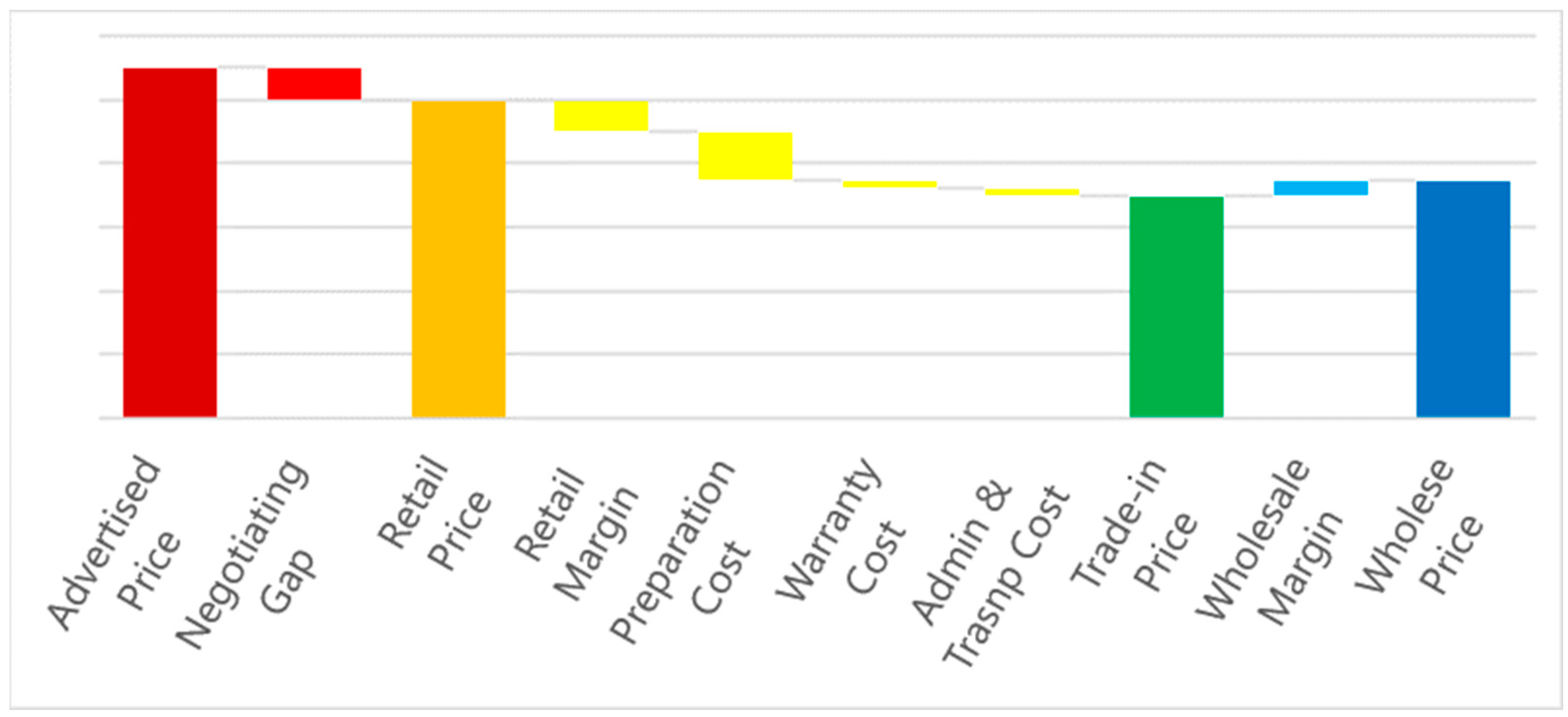
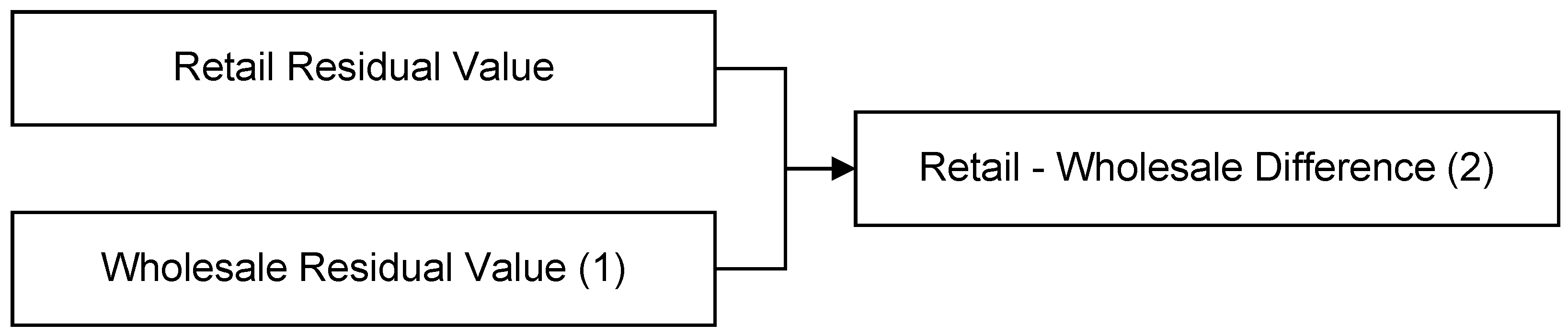
When the used machine is traded in as a payment in kind, the purchaser will make the acquisition in price, as the purchaser will have to incur preparation costs (from a minor scheduled maintenance to a mayor refurbishment) and warranty costs as well as administrative and transportation costs. This will leave a margin gap between those costs (trade-in or acquisition, preparation, warranty, and admin and transport) and the retail price that is the fair market value (FMV). Trying to sell above the fair market value implies more days in inventory with all its associated financial costs and residual value dilution. The machine is then promoted at an advertised price that leaves some room for negotiation above the retail price or FMV. The wholesale price will be lower than the retail price [5], as the sales terms and conditions will most likely be “as is, where is”, thus not including preparation, warranty administrative, or transport costs, and the margin expectations will be lower; therefore, the transactional price will reflect the different value proposition (Figure 1).
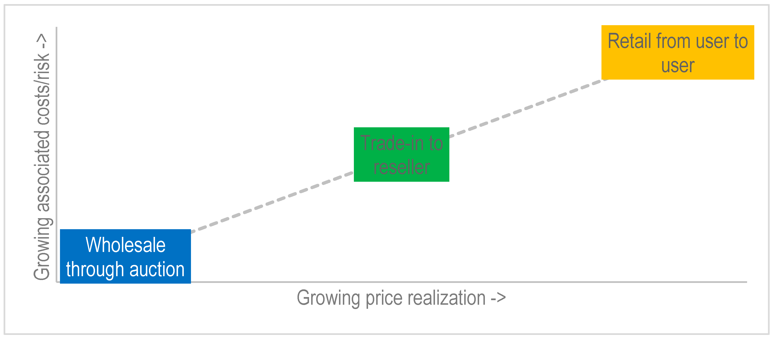
The different asset realization alternatives available at the end of the ownership cycle, including retailing it directly from the current user to another end user, trading it in as payment in kind to a reseller, or wholesaling it through an auction, provide different levels of price realization (output) by means of different levels of associated costs and risks (inputs) (Figure 2).
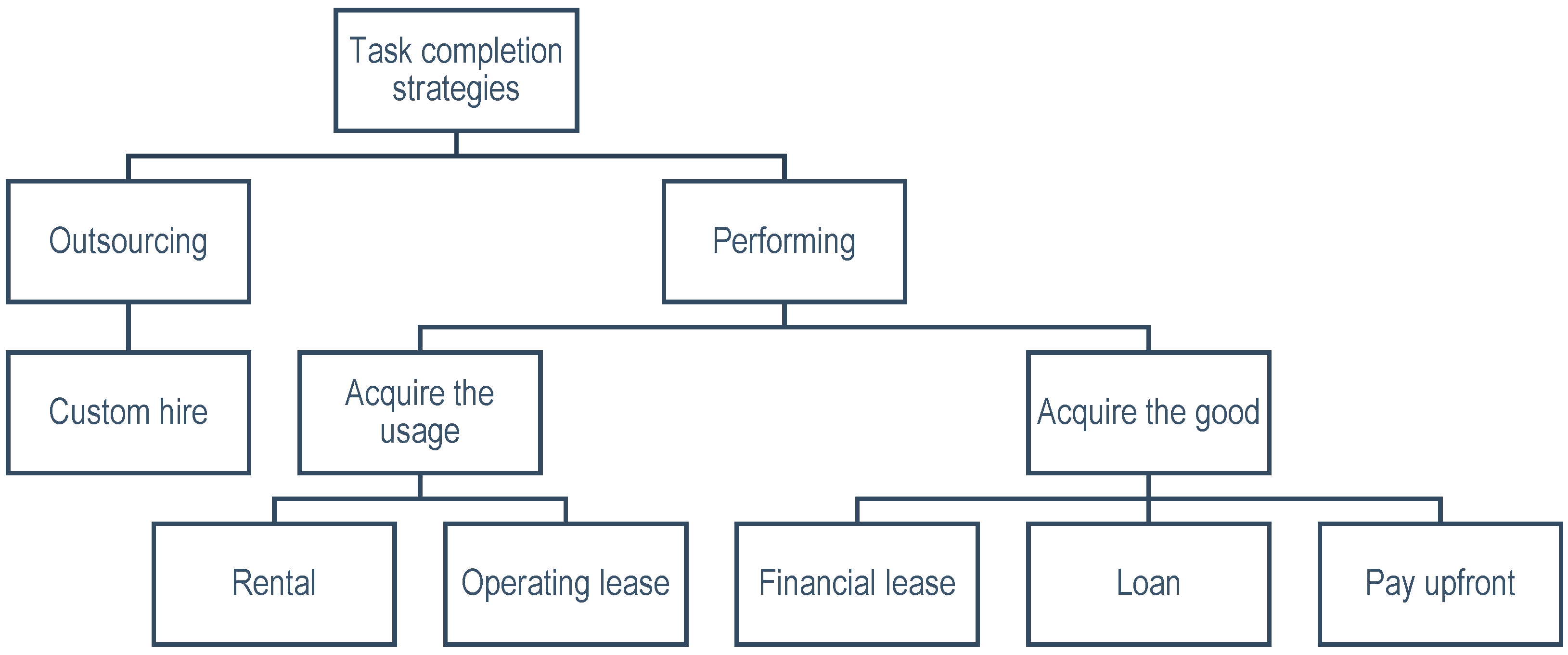
Hence, when making a judicious decision about the task completion strategies that Figure 3) predicated on the factual information, it becomes imperative to meticulously deliberate upon all potential avenues for asset realization, encompassing both output and input aspects. This thorough evaluation should encompass all considered brands and models, taking into account the salient attributes that exert the greatest influence on pricing. By doing so, one can effectively determine the comprehensive ownership costs with the utmost precision, thereby attaining optimal asset functionality and, subsequently, enhancing the overall financial performance of the enterprise.
In recent years, the research pertaining to the forecasting of residual values in the retail sector, particularly using auction results as a data source, has been relatively scarce. The available studies in this domain have not provided up-to-date and comprehensive data, leaving a noticeable gap in the literature. Furthermore, among the limited research conducted, only one European study has considered auction results as a primary dataset. Additionally, there is a dearth of studies specifically focused on examining the relationship between wholesale residual values and retail residual values. This gap in the literature underscores the pressing need for a comprehensive study that not only facilitates the forecasting of retail residual values but also delves into wholesale residual values and elucidates the disparities between them. Addressing this research gap is of paramount importance, as it equips stakeholders with vital insights for making data-driven decisions that optimize their databases.
1.1. Previous Studies
The significance of a thorough comprehension of agricultural tractor depreciation rates cannot be overstated, and substantial research has been undertaken in this domain.
In 1983, Reid and Bradford [6] performed an analysis of 411 tractors in the United States and utilized exponential functions to assess the impact of the age, power, motor type, manufacturer, increasing usage, and technological advancements on the residual value. In a 1986 separate study conducted by Perry et al. [7] in the United States, 1612 tractors were examined, and the Box–Cox transformation was employed to estimate the influence of factors such as the age, power, manufacturer, usage, care, and macroeconomic variables on the residual value. Similarly, in 1991, Hansen & Lee [8] investigated agricultural tractors in Canada and employed a linear function to ascertain the relationship between the age, year of manufacture, and purchase year and the residual value.
Cross and Perry [9,10] used Box–Cox transformations to estimate the effects of the age, hours of use, brand, condition, auction region and type, and economic macro indicators on the residual value in auctions of agricultural tractors in the USA. In 1996, Unterschultz & Mumey [11] conducted a study on 3202 tractors in auctions in the USA and Canada, which was corroborated by the Hansen and Lee model. In 1996, Cross & Perry [9] studied auctions of 433 tractors with less than 60 kW, 1946 tractors between 60 and 112 kW, and 866 tractors with more than 112 kW in the USA and used Box–Cox transformations to estimate the effects of the age, hours of use, brand, condition, and economic macro variables on the residual value.
In 2004, Wu & Perry [12] conducted a study on 657 tractors with 30–79 horsepower, 1420 tractors with 80–120 horsepower, and 781 tractors with 121+ horsepower in auctions in the USA and used Box–Cox transformations to estimate the effects of the age, production year, manufacturer, and other variables on the residual value. Fenollosa & Guadalajara [13] studied 7876 tractors with 13–79 horsepower, 3963 tractors with 80–133 horsepower, and 731 tractors with 134–263 horsepower in sales in Spain from December 1999 to December 2002 and used ordinary least squares (OLS) and Box–Cox transformations to estimate the effects of the age, power, brand, and other variables on the residual value.
In 2004, Wilson & Tolley [14] and, later on, in 2010, Wilson [15] analyzed tractor advertisement data from the UK, adding Box–Cox transformations to improve the accuracy of the results. The American Society of Agricultural and Biological Engineers [16] conducted a study in 2011, based on data from the USA, considering factors such as the age, usage, and power, using Box–Cox transformations for data normalization. In 2020, Kay et al. [17] updated their analyzed auction data from the USA, applying the ASABE standards from 2006 [18].
In 2022, Witte et al. [19] analyzed advertisement and auction data from Germany, focusing on factors such as the age, usage, available power, and manufacturer, using exponential regression analysis. Also in 2022, Ruiz-Garcia & Sanchez-Guerrero [20] analyzed advertisement data from Europe, focusing on new and used tractors, and considering factors such as the age, usage, available power, and manufacturer. They used robust linear (polynomial) regression to estimate the residual value.
Finally, in 2023, Herranz-Matey & Ruiz-Garcia [21] examined advertisement data from Europe, considering factors such as the age, hours, brand, and tractor cohort, using power linear regression analysis. The current study builds upon these previous efforts by proposing a novel model that achieves highly robust results in terms of estimating the residual value of agricultural tractors. The model confirmed its robustness and sturdiness using more limited-in-numbers combined advertisements [22].
The lack of sufficiently abundant transactional European information to enable robust modeling leads all studies to focus on advertised tractors. The populace, classification, and condition of agricultural machinery sold through European auctions may not solely reflect the market value of a second-hand tractor as offered by a proficient vendor. Nonetheless, such data can furnish useful insights into, and enhance our comprehension of, the residual value trends.
Witte et al. [19] not only pioneered by considering both the advertised and auctioned prices but also discussed the importance of having a good understanding of the auctioned price and how it relates to the retailed (advertised) price.
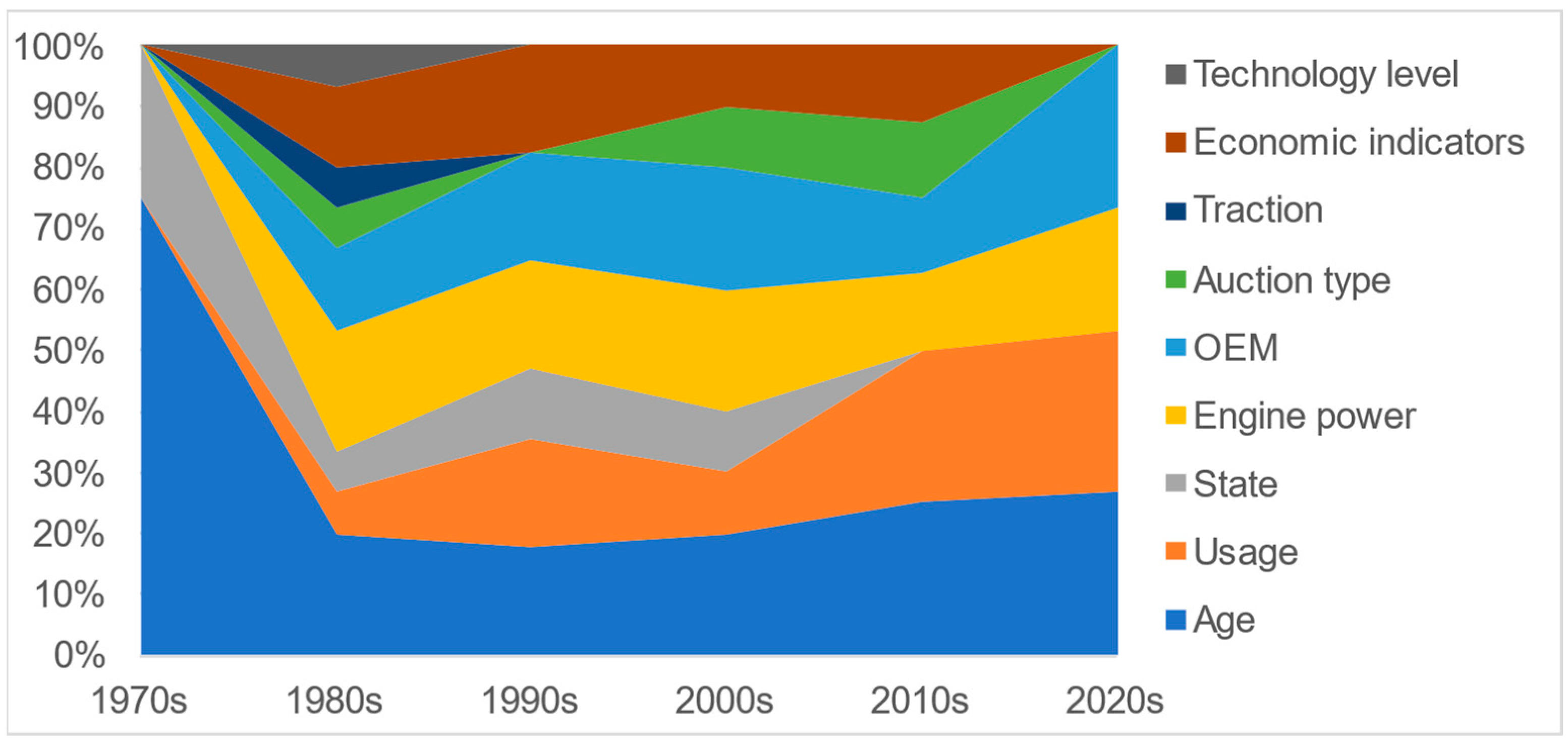
Residual value analysis investigations have encompassed a spectrum of factors that have evolved over time, as depicted in (Figure 4).
During the 1970s, analyses primarily relied upon age and the condition of the tractor, as discerned from transactional data provided by dealers’ associations. As original equipment manufacturers (OEMs) expanded and diversified their product portfolios by incorporating a wider array of features and specifications, an expanded set of variables were integrated, including elements such as usage patterns and the engine power. This transition occurred concurrently with a decline in the availability of transactional data sourced from dealer associations in the North American context, thereby prompting researchers to turn to auction outcomes as a data source.
In an effort to amass more substantial and comprehensive datasets, subsequent investigations turned to longitudinal data collected over multiple years. This expansion necessitated the inclusion of economic indicators alongside variables such as the traction type, e.g., two-wheel drive (2WD) or mechanical forward wheel drive (MFWD), and technological sophistication, e.g., cabbed, or open operator stations. As the research shifted from a reliance on dealer association pricing guides to the utilization of auction data, the imperative to incorporate data from multiple years diminished somewhat. However, with the widespread proliferation of auctions, the need arose to differentiate between diverse auction types, encompassing repossessions, bankruptcies, retirements, etc. More recent examinations have homed in on the age, usage, engine power, and OEM factor as the primary determinants of the residual value.
Throughout the past few decades, a discernible trend in residual value forecasting studies has comprised a substantial reduction in the number and typology of the selected variables, with a consistent focus on a core set of four variables: the age, usage, power, and OEM (original equipment manufacturer). The unanimous preference for this parsimonious selection of variables can be attributed to the observed enhancement in result robustness across all instances of their application.
Acquiring a lucid comprehension of the auction-derived value pertaining to agricultural tractors holds paramount significance for all stakeholders involved. This insight offers a tangible grasp of the pricing benchmarks that might be challenged in scenarios involving unforeseen mechanical failures, catastrophic or otherwise, or in situations necessitating a prompt price realization.
1.2. Curent Issues
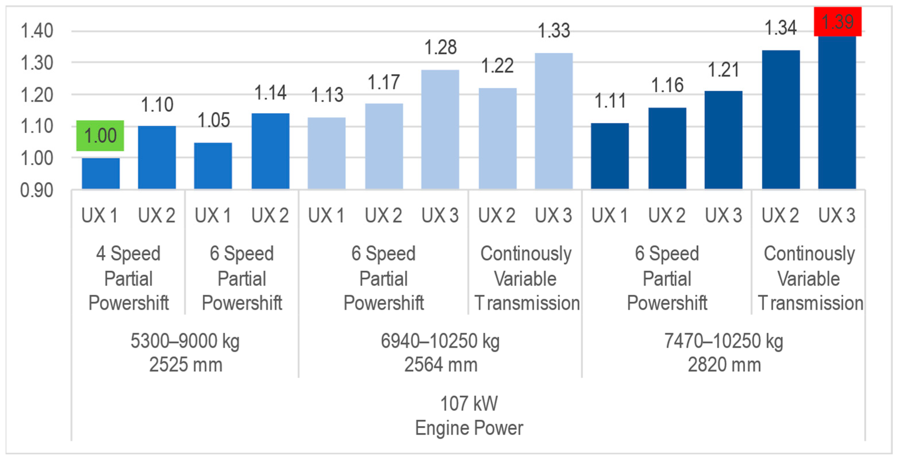
In their 2023 study, Herranz-Matey, and Ruiz-Garcia [21] highlight the fact that manufacturers of tractors offer assorted sizes and features within the same power category, which leads to price differences of up to 39% between models (Figure 5). This suggests that the power is not the only or even the most crucial factor driving the price of tractors. Instead, other factors, such as the size, features, and brand, may play a more significant role in determining the price of a tractor.
The authors also note that compliance with European Commission off-road diesel engine emission regulations [23,24,25,26] has been a major concern for the tractor industry in recent years. However, they argue that the associated costs of complying with these regulations have not been the primary driver of price increases. This finding is supported by previous studies showing that the technical solutions required for diesel engine emission regulation compliance have a significant cost that has increased the tractor price with the implementation of each regulation stage [27,28].
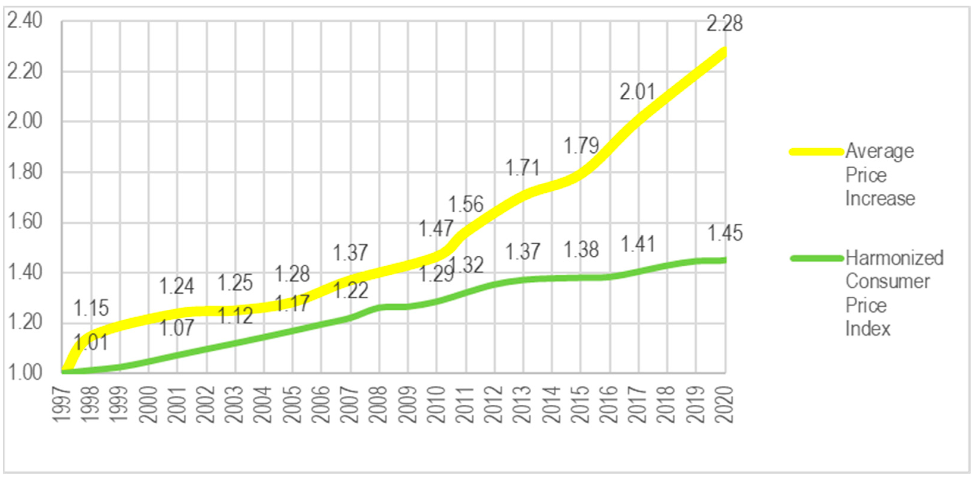
The agricultural tractor price increase due to diesel engine emission regulation compliance since the different stages of implementation has always been considerably higher than the Harmonized Index of Consumer Prices (Figure 6).
The current study addresses the lack of studies forecasting the wholesale residual value. The number of auctions that take place in Europe, although gaining momentum, is somewhat smaller than that in North America, where it is a normal practice; thus, the studies that consider auction transactional data are scarce [19]. Therefore, this study innovates by developing, firstly, a new wholesale residual value model based on a different dataset type source (auction sales results) and, secondly, a novel model to calculate the difference between the residual value of the same equipment when retailed and when wholesaled (Figure 7).
2. Goal
The objective of this study is to develop a robust residual value model (1) that is user-friendly (2) and can be implemented using mainstream software that is widely accessible (3) to all residual value stakeholders, including manufacturers, sellers, financers, insurers, and users.
The envisaged model will provide stakeholders with the capability to accurately compute the wholesale residual value, as well as discerning the differentials that exist between wholesale and retail residual valuations. This equitable provision of knowledge acts to level the playing field amongst these stakeholders, particularly in light of the constraints surrounding access to transactional historical data. It is noteworthy that such accessibility is either restricted or selectively disseminated to a subset of these stakeholders, resulting in an uneven distribution of residual value insights.
Through the deliberate examination of the wholesale market as a viable alternative to the retail counterpart, stakeholders will be duly empowered to effect judicious decisions pertaining to the acquisition of both new and pre-owned agricultural tractors. This strategic empowerment, in turn, augments their capacity to optimize their financial performance through well-informed choices.
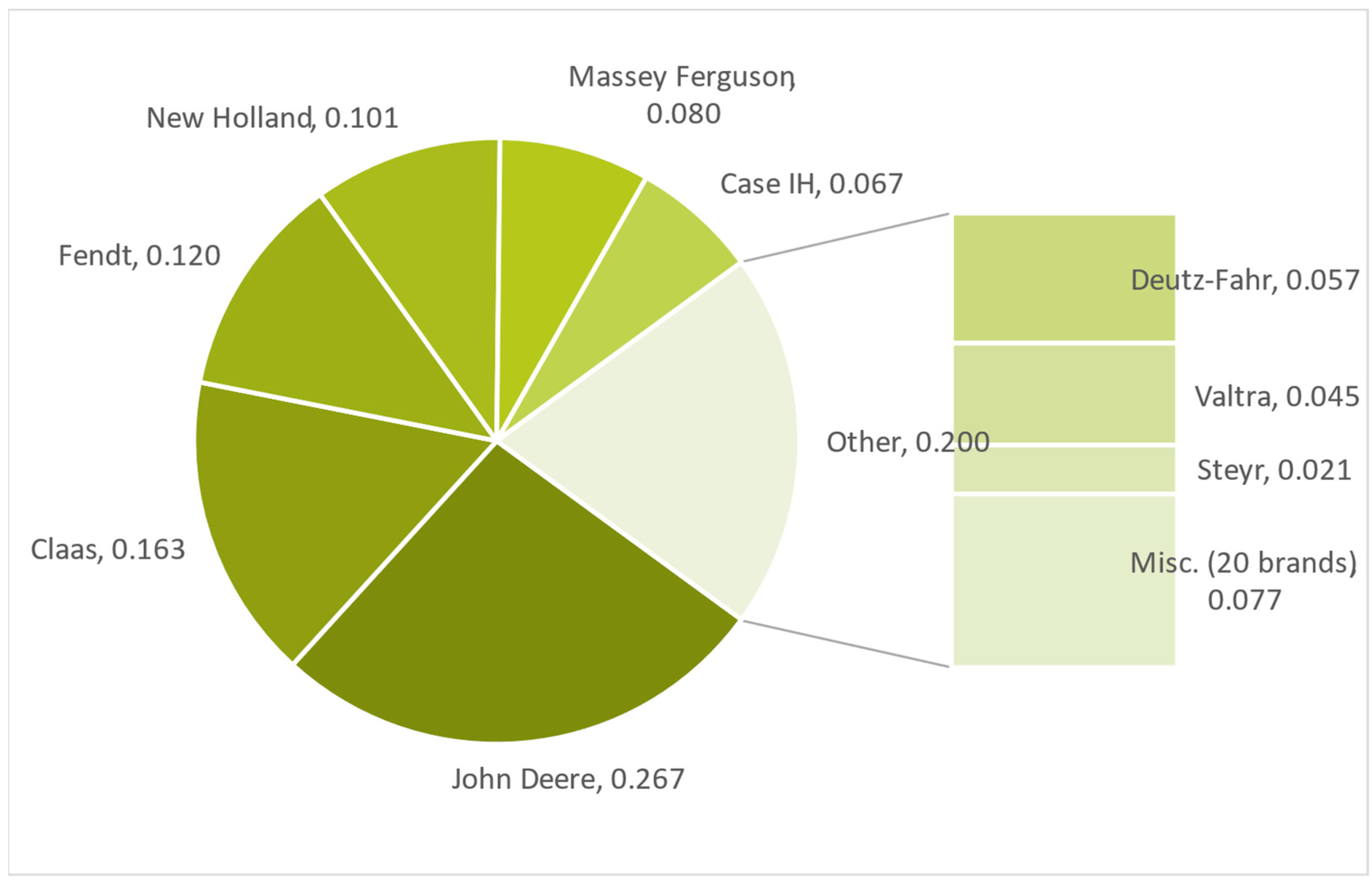
To achieve this objective, a residual value calculation methodology will be designed that strikes a balance between simplicity of usage and precision of results. The proposed methodology will be applicable to standard agricultural tractors with an engine power above 75 kW, featuring a cab, and manufactured by the primary OEMs, including Case IH, Claas, Fendt, John Deere, Massey Ferguson, and New Holland, which represent 80% of the new and used equipment market (Figure 8) in the primary Western European markets [29] (Figure 9).
This model aims to serve all interested parties, including users, producers, finance and insurance entities, financiers, and insurers, by providing an accessible and effective tool for calculating residual values [29].
3. Materials and Methods
3.1. Dataset
In congruence with the present discourse, it is imperative to underscore the adherence to temporal consistency in methodological design, akin to the investigative approach undertaken by Witte et al. This current investigation is delimited to the domain of agricultural tractors, specifically those commercialized under the brands New Holland, Massey Ferguson, John Deere, Fendt, Claas, and Case IH, and with an engine power surpassing seventy-five kilowatts. The geographic scope of observation encompasses Germany, the United Kingdom, France, Spain, and Italy, spanning the contiguous previous 18-month interval, a temporal framework that closely mirrors the pioneering work of Witte et al. [19].
This temporal interval facilitates the acquisition of a dataset of significant magnitude. However, the restricted quantity of auctioned machinery hinders the attainment of a dataset of desirable proportions spanning a more optimal duration of 12 months. Such a duration would encompass both an agricultural year and an original equipment manufacturer (OEM) marketing year. This is particularly pertinent due to the influence of discount and incentive initiatives on new equipment pricing and financing within the agricultural machinery sector.
The rationale underlying the selection of this specific duration is twofold: foremost, it aims to secure a sufficiently voluminous dataset, thereby engendering a robust statistical power; secondarily, it seeks to circumvent the potential influence of swiftly fluctuating economic conditions. The primary repository of data acquisition emanated from an authoritative online source (https://www.rbauction.com/heavy-equipment-auctions/past-auctions), with data retrieval taking place on the 15 July 2022.
The dataset under consideration encompasses a distinct and unique set of 1120 observations derived from tractor auction transactions specifically for this study. These observations have been meticulously categorized exclusively for the purposes of this particular study. This dataset offers a substantial and unique repository of information, providing fertile ground for the comprehensive analysis of the agricultural tractor market within the geographical regions of interest. This compilation holds the potential to unearth valuable insights into discernible trends and intricate patterns pertaining to tractor manufacturers, incorporated features, and pricing dynamics.
3.2. Data Systemization and Processing
The determination of the residual value (RV), as originally conceptualized by Herranz-Matey and Ruiz-Garcia [21], can be ascertained through the following computational process:
Utilizing the identical tractor cohort grouping criterion, which categorizes tractors based on their size attributes (including the wheelbase and minimum and maximum mass) and technological features (inclusive of transmissions and user interfaces), and, in certain instances, necessitates the division of manufacturer-defined tractor series into distinct cohorts, we employ a novel approach known as the “new equivalent tractor method”. This method involves establishing correspondence with all the predecessors of each individual model within every cohort, spanning the specified timeframe dating back to 1998. This correspondence is determined via considering the relative model positioning within the tractor series, as well as the distinctive features associated with each model. The current manufacturer portfolio offering is complex [21], to the point that, for example, one 100 kW tractor can feature from 2.420 to 2.820 m and from 6.750 to 10.650 kg (Figure 10), rendering the engine power less decisive in price realization.
3.3. Data Analysis
3.3.1. Wholesale Residual Value Regression
This study aimed to evaluate alternative regression options by analyzing various models and subtypes, including bagged and boosted tree ensembles; exponential, Matérn 5/2, rational quadratic, and squared exponential Gaussian process regression (GPR); least-square regressions and supported vector machine kernels; linear and robust linear regressions; bilayered, medium, narrow, trilayered, and wide neural networks; coarse and fine Gaussian; cubic, linear, median and quadratic supported vector machines (SVMs); and fine and medium trees (Figure 11).
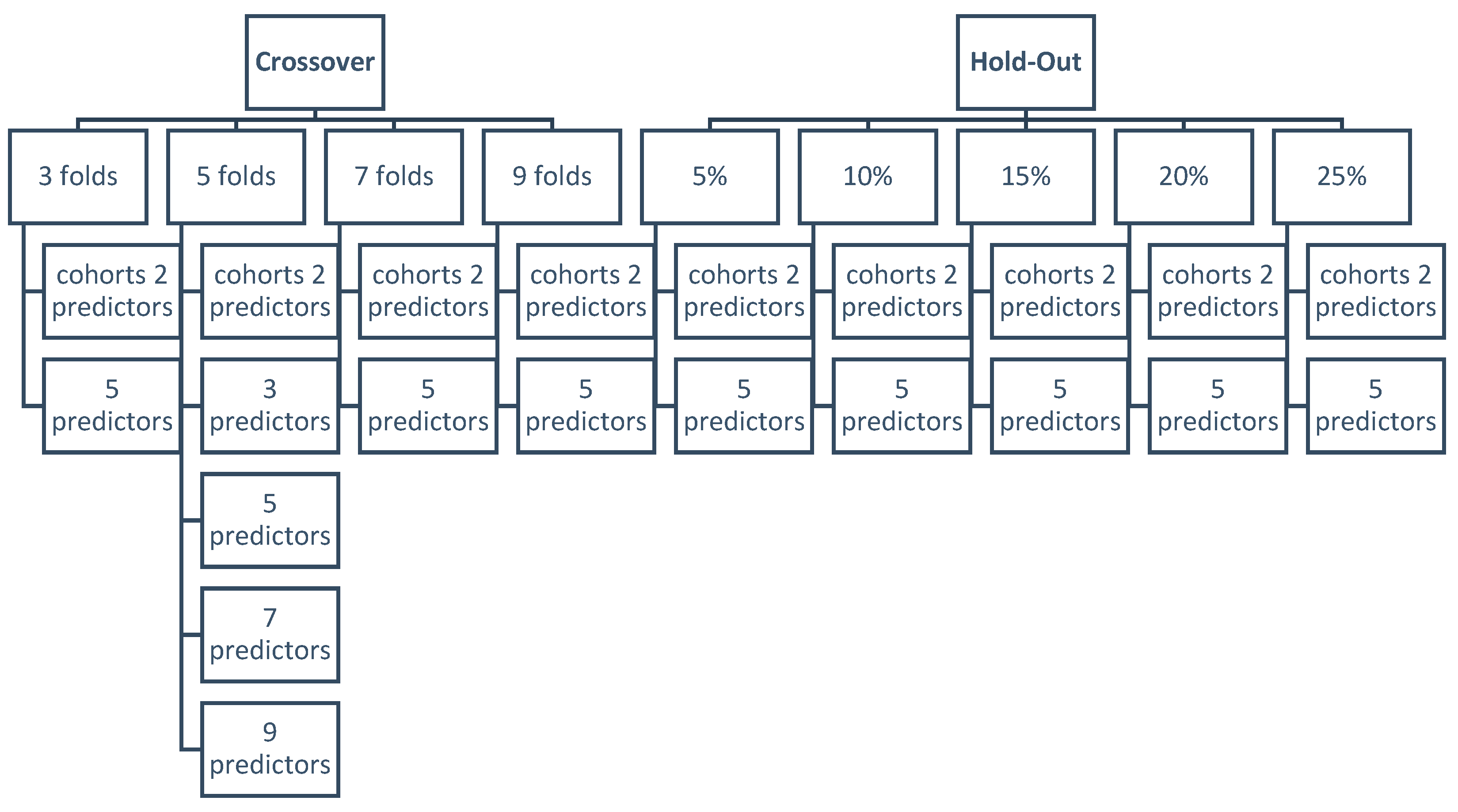
The above-mentioned fitted models were tested with 2, 3, 5, 7, and 9 predictor variables, including the age, hours, tractor cohort, model, current equivalent model, brand, country, wheelbase, and engine power. Both crossover validation (with 3, 5, 7, and 9 folds) and hold-out validation (with 5%, 10%, 15%, 20%, and 25% test data) were employed, using machine learning optimization (Figure 12).
As already mentioned, as the OEM product portfolio has increased its complexity, the power has lost relevance as a price driver, as OEMs offer multiple models with the same power but a very different wheelbase and mass (Figure 5) and featured transmission type and user interfaces that provide different productivity and reliability and, hence, a different customer perception, which drives diverse residual value behaviors for different models of the same OEM with the same power.
As previously elucidated, the practice of categorizing tractor models into tractor model cohorts serves to consolidate attributes such as the wheelbase, mass, transmission features, and user interfaces, thereby fostering a greater homogeneity within the dataset. The assessment of residual values for these tractor models, organized into cohort groups, is contingent upon the analysis of two key variables, namely, the operating hours and age. To predict the residual values, a comprehensive examination of both non-parametric and parametric models has been undertaken, with the following models being subject to evaluation.
In evaluating the performance of the model, two metrics have been employed, namely the root-mean-square error (RMSE) and the adjusted coefficient of determination (RSqAdj). The choice of the RMSE is based on the need to present errors in the same unit as the outcome variable to facilitate easy interpretation. A model that is 100% accurate will have an RMSE value of zero. Conversely, the RSqAdj has been used to account for the portion of variance in the dependent variable that is explained by the regression model, taking into consideration the number of predictor variables used to predict the dependent variable [30].
3.3.2. Retail and Wholesale Residual Value Difference Regression
Once the retail and the wholesale residual value can be predicted, it is remarkably simple to calculate the difference with the following equation:
The difference between the retail regression value and the wholesale regression value is calculated for ages from 1 to 20 years, in 1-year increments, and from 100 to 750 h per year (HPY) in 50 h increments.
4. Results
4.1. Wholesale Residual Value Regression
Consistent with the findings corroborating the methodology and model as previously reported in references [21,22], and in accordance with the results elucidated in Table 1, Table 2, Table 3 and Table 4, the power regression model (4) demonstrated the most favorable performance when assessed using both the RMSE and RSqAdj metrics. Therefore, it is the regression model recommended for adoption.
The advanced models that were tested demonstrated that those with seven predictors yielded superior RMSE values when compared to models (Figure 11) with three, five, or fewer predictors (Figure 12). Moreover, models that utilized hold validation outperformed those that utilized cross-validation. The exponential Gaussian process regression model with seven predictors and a 10% holdout validation exhibited the best overall performance, with an RMSE of 0.0518 (Table 2).
Given that the proposed methodology focused on power regression models with only two predicting variables for tractor cohorts, it was important to explore more advanced models that could leverage more complex models. Hence, the tractor families that rendered the best power regression model RMSE results were tested using the same fitted models with a 10% hold-out validation to provide datasets. The best overall model across most family groups was the optimized Gaussian process regression (OGPR).
Despite employing machine learning techniques for model enhancement, it is noteworthy that the utilization of parametric regression yielded outcomes characterized by an increased resilience. This study harnessed a dual set of predictors in conjunction with a 10% holdout validation procedure within the domain of the considered tractor cohorts. The yielded outcomes, encompassing the root-mean-square error (RMSE) and adjusted R-squared (RSqAdj) metrics, exhibited a degree of satisfaction that can be classified as notably elevated.
Significantly, the outcomes emanating from the implemented power (log–log) regression model, devised through the amalgamation of two predictors meticulously categorized based on their corresponding cohorts (effectively consolidating the dataset with closely aligned characteristics in terms of size, including the wheelbase and mass, as well as technical specifications involving the transmission and user interface) reduced the extraneous variability and facilitated a focused analysis of pertinent variables, such as the age, hours, and price. These outcomes demonstrated a level of superiority that surpassed even the most precise regression model fine-tuned through the sophisticated techniques of machine learning optimization (Table 3).
The proposed power (log–log) regression model exhibited a high degree of precision in tracking the residual value behavior across different tractor cohorts. Furthermore, the fact that the second-best performing model was exponential regression, as previously noted by [19], suggests that these models outperform more complex models, such as optimized Gaussian regressions (OGPRs).
4.2. Retail and Wholesale Residual Value Difference Regression
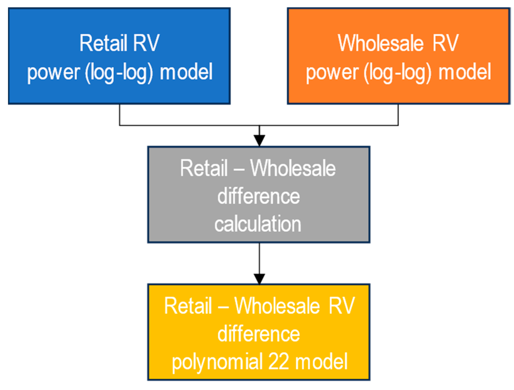
As the calculation of the retail residual value forecasts relies upon the implementation of a power (log–log) regression method (as delineated by Herranz-Matey and Ruiz-Garcia [21]), and as the aforementioned methodology and model have consistently delivered robust wholesale residual value forecasts, the computation of the disparity between the forecasted retail and wholesale residual values becomes a straightforward task (Figure 13).
The next goal of this study is to forecast the difference between the retail and wholesale residual values (Figure 14).
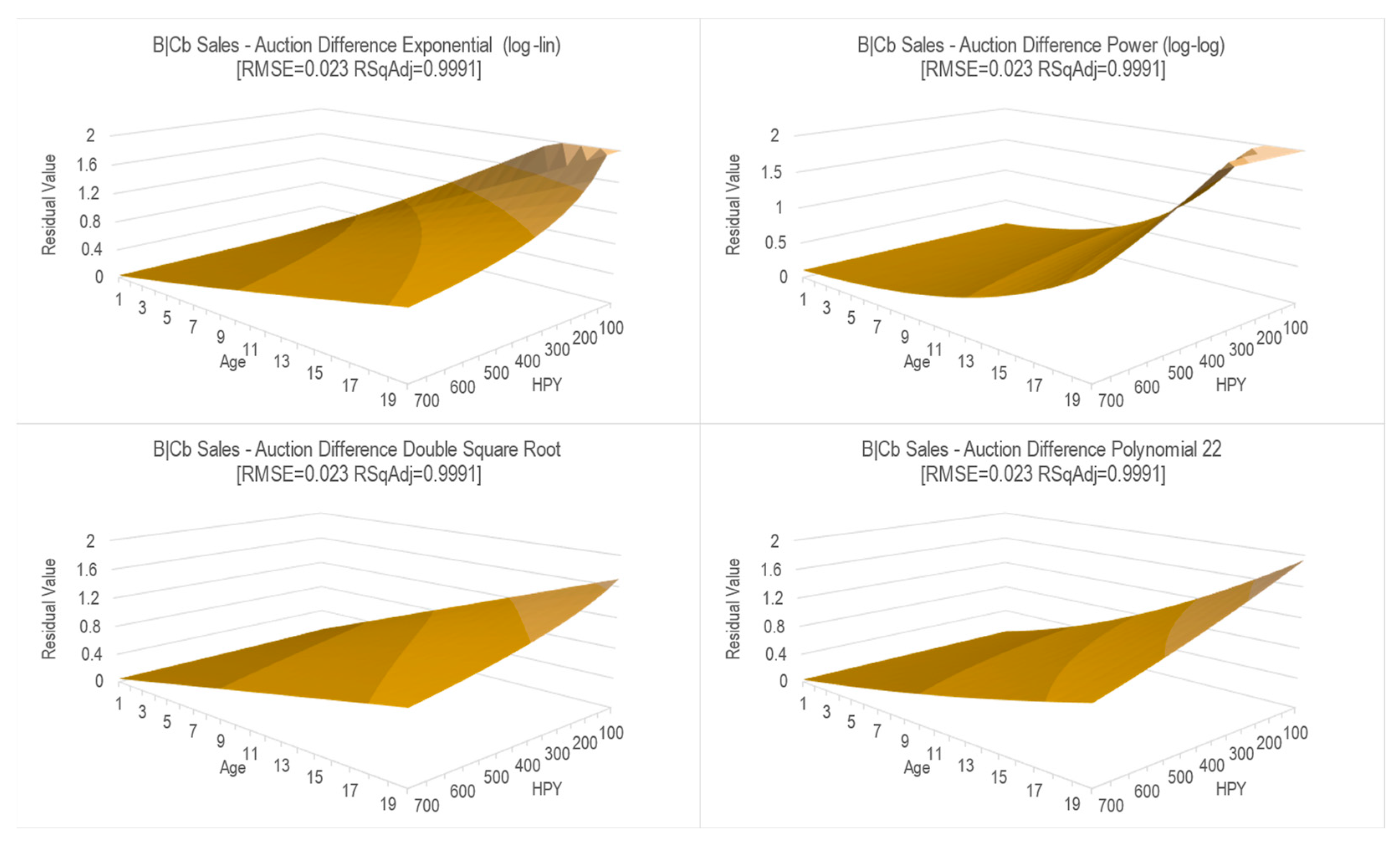
The objective of this analysis was to achieve the highest level of precision in forecasting the disparity between the wholesale and retail residual values. To ascertain the most suitable model for predicting the difference between the retail and wholesale residual values, which constitute the two predictive parameters, a comprehensive examination, encompassing a spectrum of regression models, has been conducted. These models encompassed linear (lin–lin) (2), logarithmic (lin–log) (3), power (log–log) (4), exponential (log–lin) (5), double square root (6), polynomial 12 (7), polynomial 21 (8), and polynomial 22 (9) regression models.
The surface graphs represent the B|Cb tractor cohort retail and wholesale residual value difference regression lowest-RMSE models (Figure 15). Visualized are the regression model results and how they compare to the actual difference, showing the best correlation using polynomial 22 regression (9), compared to exponential (log–lin) (5), power (log–log) (4), and double square root (6).
5. Discussion
5.1. Wholesale Residual Value Regression
The proposed power regression model exhibits a higher level of predictive robustness compared to previous studies that have relied solely on age and usage hours, as well as brand and power features, to predict residual value behavior. It is worth noting that power alone may not be sufficient to differentiate residual value behavior, particularly for tractor cohorts from the same brand with similar power ratings but differing sizes, masses, transmissions, and user interfaces, as highlighted by Herranz-Matey & Ruiz-Garcia [21]. In contrast, the proposed model considers these factors by delving into the modeling level and grouping tractors into cohorts, resulting in a more solid foundation for robust results that outperform those of previous studies based on auction data (Table 5).
The present study has put forth a methodology that employs a straightforward approach and delivers superior root-mean-square error (RMSE) and adjusted R-squared (RSqAdj) outcomes compared to advanced fitting models that necessitate specialized software. Moreover, the proposed technique is highly amenable to mainstream software, which renders it accessible to a wider audience.
The methodology and model elucidated by Herranz-Matey and Ruiz-Garcia (Reference [21]) exhibited a commendable degree of robustness. To scrutinize the origins of this robustness, particularly whether it stemmed from the ample size of the advertised tractor dataset (exceeding 10,000 units) or from the inherent attributes of the methodology and model themselves, Herranz-Matey and Ruiz-Garcia (Reference [22]) subjected the methodology and model to a rigorous evaluation using a more limited and diverse dataset comprising 1197 advertised combines of various machine types. Subsequently, the authors undertook a second challenge, employing a smaller dataset consisting of 1120 entries from a distinct data source—auctions, in lieu of advertisements. These subsequent challenges served to corroborate the ease of use, adaptability, and resilience of the methodology and model.
The methodology and model necessitate the availability of ample information to establish a chronological framework for the equivalent new model and to determine the portfolio size required for the categorization of cohorts with analogous specifications (such as the mass and wheelbase) and features (including the transmission and user interface). This categorization is essential to ensure an adequate population of data.
5.2. Retail and Wholesale Residual Value Difference Regression
In 2022, Witte et al. [19] not only pioneered by considering both advertised and auctioned prices but also discussed the importance of having a good understanding of the auctioned price and how it relates to the retailed (advertised) price. Witte et al. (2022) used both advertised and auction prices and even stated that the average discount between advertisements and action results was 30.1%.
The proposed polynomial 22 regression model (9) offers a comprehensive analysis of the difference between retail and wholesale prices by tractor cohort, age, and usage hours, yielding a root-mean-square error (RMSE) of 0.0159 and an adjusted coefficient of determination (RSqAdj) of 0.9997.
The power (log–log) regression (4), used to determine retail and wholesale residual values, along with polynomial 22 regression (9), to determine the difference in residual values, provide valuable insights for all the stakeholders involved in the used tractor market, including manufacturers, sellers, financers, insurers, and users. The model not only considers the retail market but also widens market opportunities by forecasting values in the wholesale market, widening the asset conversion options for all the affected stakeholders.
Furthermore, the model is fueled by publicly accessible data and can be conveniently implemented with widely available software, lending it a high degree of transparency, and offering a multitude of analysis possibilities that can be swiftly visualized (Figure 16).
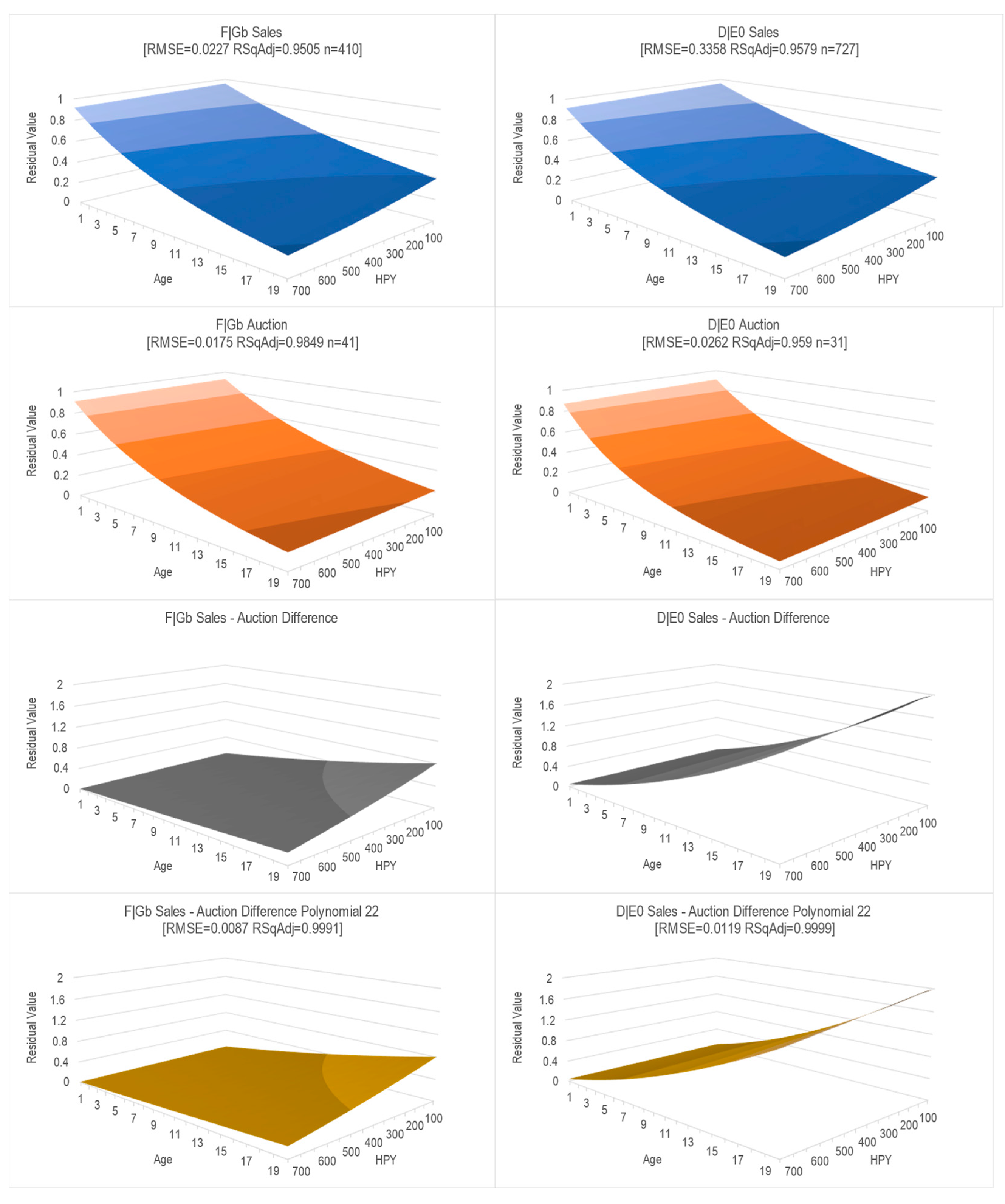
The specifications and features of the tractor and its condition might be refurbished or even improved, but this implies a used tractor cost increase that will only will be justified if it enables decision-makers to opt for the retail market instead of the wholesale market, achieving a higher price realization (see tractor cohort D|E0 in Figure 16), or the opposite situation, in case the cost of that refurbishment, or improvement, overcomes the potential price realization derived from the retail price compared to the wholesale price (see cohort F|Gb in Figure 16).
6. Conclusions
The proposed power (log–log) regression model, as applied to the estimation of the wholesale residual values, is distinguished by its pronounced robustness, a characteristic that transcends antecedent inquiries and even surpasses more sophisticated methodologies entailing the employment of machine learning optimization techniques.
This ascendancy can be attributed to a confluence of factors. To begin with, the model undertakes a discrete examination of each individual tractor model, thereby effectuating the eradication of extraneous influences arising from other tractor models possessing commensurate power levels albeit distinctive specifications. Furthermore, the model systematically accommodates the fluctuations in pricing that result from evolving emission regulations and variations in specifications by virtue of a meticulous juxtaposition between the resale prices of pre-owned tractors and the corresponding figures pertaining to their new counterparts.
In addition to this, recognizing the potential challenge posed by constrained statistical data, the model adopts a stratagem wherein tractor models are either aggregated into coherent cohort clusters in instances of scanty sample sizes or, alternatively, disaggregated into more delimited subgroups in cases when the dataset proves sufficiently extensive and substantive differentials exist amongst models within the same series.
The proposed methodology, anchored in a power (log–log) linear regression model predicated on tractor cohort group new equivalent models, has demonstrated its substantial robustness in the prediction of retail residual values for tractors and combines, as previously established in earlier studies. Moreover, when extended to the realm of wholesale data obtained from auctions, this model has exhibited a superior resilience in contrast to preceding investigations and sophisticated machine learning optimized models (with an observed RMSE of 0.0695 and an RSqAdj of 0.8461). Noteworthy is its user-friendly nature, requiring only a rudimentary internet search on platforms specializing in pre-owned equipment and minimal interaction with sellers for data procurement, thereby streamlining the information-gathering process. Subsequently, this information can be processed transparently through widely accepted software, facilitating its accessibility and usability for a diverse spectrum of users.
Furthermore, this study takes a major stride forward by computing the disparity between the projected retail and wholesale residual values through a straightforward calculation meticulously delineated by a polynomial regression model (with a remarkable RMSE of 0.0159 and an impressively high RSqAdj of 0.9997). This analytical approach allows a practical means for all vested stakeholders to optimize their selection of the most efficacious marketing channel, be it retail or wholesale, with the aim of attaining the highest price realization. By facilitating an expeditious and straightforward comparison between retail and wholesale asset realization alternatives, this approach empowers stakeholders to make informed decisions to enhance their financial outcome.
This study’s proposed user-friendly methodological approach, grounded in publicly available information, has culminated in the construction of a robust model that leads to outcomes of substantial reliability. These outcomes hold profound significance for an array of stakeholders, encompassing end-users such as farmers, ranchers, and contractors, as well as manufacturers, resellers, financiers, and insurers. This model facilitates the accurate determination of the cost of ownership pertinent to agricultural tractors, thereby empowering these stakeholders to deliberate upon and select the most appropriate ownership strategy. This strategic selection encompasses the consideration of diverse options, including custom hiring, rental arrangements, operating leases, finance leases, conventional loans, or upfront payments.
In addition, the model aids in the identification of the optimal approach for asset conversion, spanning possibilities such as retail transactions from user to user, trade-ins with resellers as a payment in kind, or wholesale transactions via auctions. Through this multifaceted analysis, the model’s insights converge to optimize asset performance and, in turn, engender a maximized enterprise performance.
Finally, it would be highly pertinent to investigate whether the methodology and model presented in this study can be extended to other agricultural machinery types, such as self-propelled forage harvesters and combines, with comparable outcomes; therefore, further research is warranted in this area.
Author Contributions
Conceptualization, I.H.-M.; methodology, I.H.-M. and L.R.-G.; validation, I.H.-M.; formal analysis, I.H.-M. and L.R.-G.; investigation, I.H.-M. and L.R.-G.; resources, I.H.-M.; data curation, I.H.-M.; writing—original draft preparation, I.H.-M. and L.R.-G.; writing—review and editing, I.H.-M. and L.R.-G.; supervision, L.R.-G. All authors have read and agreed to the published version of the manuscript.
Funding
This research did not receive any specific grant from funding agencies in the public, commercial, or not-for-profit sectors.
Institutional Review Board Statement
Not applicable.
Data Availability Statement
If necessary, we can provide the raw data.
Acknowledgments
The authors thank Pilar Linares for her support and “Tractores y Máquinas” (https://www.tractoresymaquinas.com) for providing the IT infrastructure for this study.
Conflicts of Interest
The authors declare no conflict of interest.
References
- Kastens, T. Farm Machinery Operations Cost Calculations; Kansas State University: Manhattan, KS, USA, 1997. [Google Scholar]
- Edwards, W. FM1900/AgDM A3-30, Replacement Strategies for Farm Machinery; Iowa State University: Ames, IA, USA, 2019. [Google Scholar]
- U.S. Consumer Financial Protection Bureau What Is a Loan to Value Ratio and How Does It Relate to My Costs. Available online: https://www.consumerfinance.gov/ask-cfpb/what-is-a-loan-to-value-ratio-and-how-does-it-relate-to-my-costs-en-121/#:~:text=The%20loan%2Dto%2Dvalue%20(,will%20require%20private%20mortgage%20insurance (accessed on 1 July 2022).
- ECB Haircuts. Available online: https://www.ecb.europa.eu/ecb/educational/explainers/tell-me-more/html/haircuts.en.html (accessed on 3 July 2022).
- Nakamura, E. Pass-Through in Retail and Wholesale. Am. Econ. Rev. 2008, 98, 430–437. [Google Scholar] [CrossRef]
- Reid, D.W.; Bradford, G.L. On Optimal Replacement of Farm Tractors. Am. J. Agric. Econ. 1983, 65, 326–331. [Google Scholar] [CrossRef]
- Perry, G.M.; Bayaner, A.; Nixon, C.J. The Effect of Usage and Size on Tractor Depreciation. Am. J. Agric. Econ. 1986, 72, 317–325. [Google Scholar] [CrossRef]
- Hansen, L.; Lee, H. Estimating Farm Tractor Depreciation: Tax Implications. Can. J. Agric. Econ./Rev. Can. D’agroecon. 1991, 39, 463–479. [Google Scholar] [CrossRef]
- Cross, T.L.; Perry, G.M. Depreciation Patterns for Agricultural Machinery. Am. J. Agric. Econ. 1995, 77, 194–204. [Google Scholar] [CrossRef]
- Cross, T.L.; Perry, G.M. Remaining Value Functions for Farm Equipment. Appl. Eng. Agric. 1996, 12, 547–553. [Google Scholar] [CrossRef]
- Unterschultz, J.; Mumey, G. Reducing Investment Risk in Tractors and Combines with Improved Terminal Asset Value Forecasts. Can. J. Agric. Econ. 1996, 44, 295–309. [Google Scholar] [CrossRef]
- Wu, J.; Perry, G.M. Estimating Farm Equipment Depreciation: Which Functional Form Is Best? Am. J. Agric. Econ. 2004, 86, 483–491. [Google Scholar] [CrossRef]
- Fenollosa, M.; Guadalajara, N. An Empirical Depreciation Model for Agricultural Tractors in Spain. Span. J. Agric. Res. 2007, 5, 130–141. [Google Scholar] [CrossRef]
- Wilson, P.; Tolley, C. Estimating Tractor Depreciation and Implications for Farm Management Accounting. J. Farm Manag. 2004, 12, 5–16. [Google Scholar]
- Wilson, P. Estimating Tractor Depreciation: The Impact of Choice of Functional Form. J. Farm Manag. 2010, 13, 799–818. [Google Scholar]
- ASAE Standard D497.7; ASABE Agricultural Machinery Management Data. American Society of Agricultural and Biological Engineers: Joseph, MI, USA, 2020.
- Kay, R.D.; Edwards, W.M.; Duffy, P.A. Farm Management, 7th ed.; McGraw-Hill: New York, NY, USA, 2020. [Google Scholar]
- ASAE EP496.3; Agricultural Machinery Management. American Society of Agricultural and Biological Engineers: Joseph, MI, USA, 2006.
- Witte, F.; Back, H.; Sponagel, C.; Bahrs, E. Remaining Value Development of Tractors—A Call for the Application of a Differentiated Market Value Estimation. Agric. Eng. 2022, 77, 3273. [Google Scholar] [CrossRef]
- Ruiz-Garcia, L.; Sanchez-Guerrero, P. A Decision Support Tool for Buying Farm Tractors, Based on Predictive Analytics. Agriculture 2022, 12, 331. [Google Scholar] [CrossRef]
- Herranz-Matey, I.; Ruiz-Garcia, L. A New Method and Model for the Estimation of Residual Value of Agricultural Tractors. Agriculture 2023, 13, 409. [Google Scholar] [CrossRef]
- Herranz-Matey, I.; Ruiz-Garcia, L. Agricultural Combine Remaining Value Forecasting Methodology and Model (and Derived Tool). Agriculture 2023, 13, 894. [Google Scholar] [CrossRef]
- European Commission (EC). EC Directive 97/68/EC of the European Parliament and of the Council of 16 December 1997; European Commission (EC): Brussels, Belgium, 1997. [Google Scholar]
- European Commission (EC). EC Directive 2000/25/EC of the European Parliament; European Commission (EC): Brussels, Belgium, 2000. [Google Scholar]
- European Commission (EC). EC Directive 2004/26/EC of the European Parliament and of the Council of 21 April 2004 Amending Directive 97/68/EC; European Commission EC: Brussels, Belgium, 2004. [Google Scholar]
- European Commission (EC). EC Directive 2009/30/EC of the European Parliament and of the Council of 23 April 2009 Amending Directive 98/70/EC; European Commission (EC): Brussels, Belgium, 2009. [Google Scholar]
- Posada, F.; Chambliss, S.; Blumberg, K. Cost of Emission Reduction Technologies for Heavy Duty Diesel Vehicles; The International Council on Clean Transportation ICCT: Washington, DC, USA, 2016. [Google Scholar]
- Lynch, L.A.; Hunter, C.A.; Zigler, B.T.; Thomton, M.J.; Reznicek, E.P. On-Road Heavy-Duty Low-NOx Technology Cost Study. In National Renewable Energy Laboratory (NREL); U.S. Department of Energy: Washington, DC, USA, 2020. [Google Scholar]
- CEMA. Economic Press Release Tractor Registrations 2021; CEMA AISBL—European Agricultural Machinery: Brussels, Belgium, 2022. [Google Scholar]
- McCarthy, R.V.; McCarthy, M.M.; Ceccucci, W.; Halawi, L. Applying Predictive Analytics; Springer International Publishing: Cham, Switzerland, 2019; ISBN 978-3-030-14037-3. [Google Scholar]
Figure 1.
Graphical depiction illustrating the interconnections among the glossary of terms.

Figure 2.
Graphical depiction illustrating the interrelation between input and output in asset realization alternatives.
Figure 2.
Graphical depiction illustrating the interrelation between input and output in asset realization alternatives.

Figure 3.
The contemporary approaches employed for the fulfillment of agricultural machinery tasks.

Figure 4.
Analysis of previous studies, considering the variable distribution, grouped by decade.

Figure 5.
The relative (most economical = 1) price positioning of marketed 107 kW tractors (different models (x3) with different wheelbases and masses, featuring different transmissions (x3), managed via different user interfaces (UX) (x3) offered by brand B.
Figure 5.
The relative (most economical = 1) price positioning of marketed 107 kW tractors (different models (x3) with different wheelbases and masses, featuring different transmissions (x3), managed via different user interfaces (UX) (x3) offered by brand B.

Figure 6.
The Harmonized Index of Consumer Prices and the average tractor price increase relative to 1997 = 1 in the Eurozone.
Figure 6.
The Harmonized Index of Consumer Prices and the average tractor price increase relative to 1997 = 1 in the Eurozone.

Figure 7.
Description of the study methodology steps (1 = innovative auction transactional data-based model, 2 = innovative specific regression model).
Figure 7.
Description of the study methodology steps (1 = innovative auction transactional data-based model, 2 = innovative specific regression model).

Figure 8.
Agricultural tractor advertised units in Europe published on scope websites, distributed by brand.
Figure 8.
Agricultural tractor advertised units in Europe published on scope websites, distributed by brand.

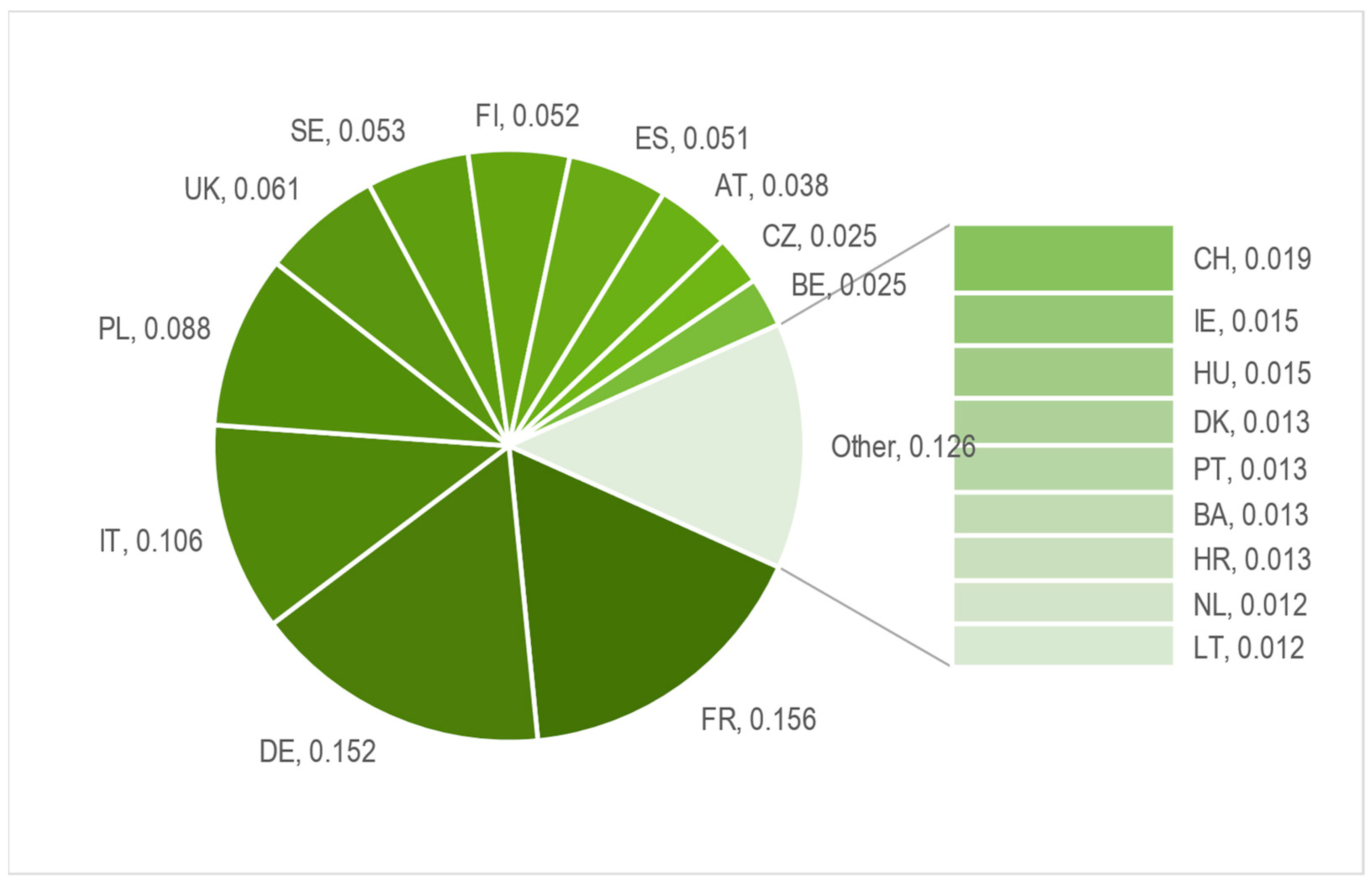
Figure 9.
The total agricultural tractors registrations units in Europe (CEMA from January to December 2020).
Figure 9.
The total agricultural tractors registrations units in Europe (CEMA from January to December 2020).

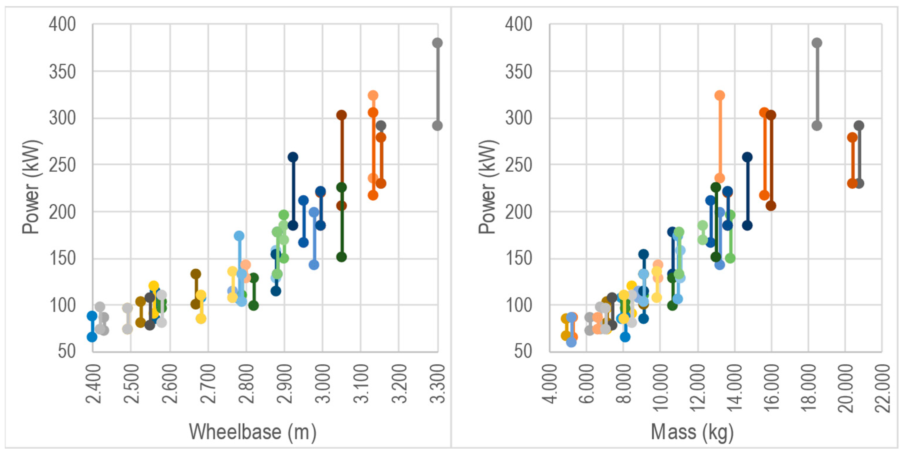
Figure 10.
The tractor model cohorts’ maximum and minimum engine power (kW), wheelbase (m), and mass (kg) distribution.
Figure 10.
The tractor model cohorts’ maximum and minimum engine power (kW), wheelbase (m), and mass (kg) distribution.

Figure 11.
The fitted models and subtypes in the study.

Figure 12.
The fitted model and subtype variables and validations in the study.

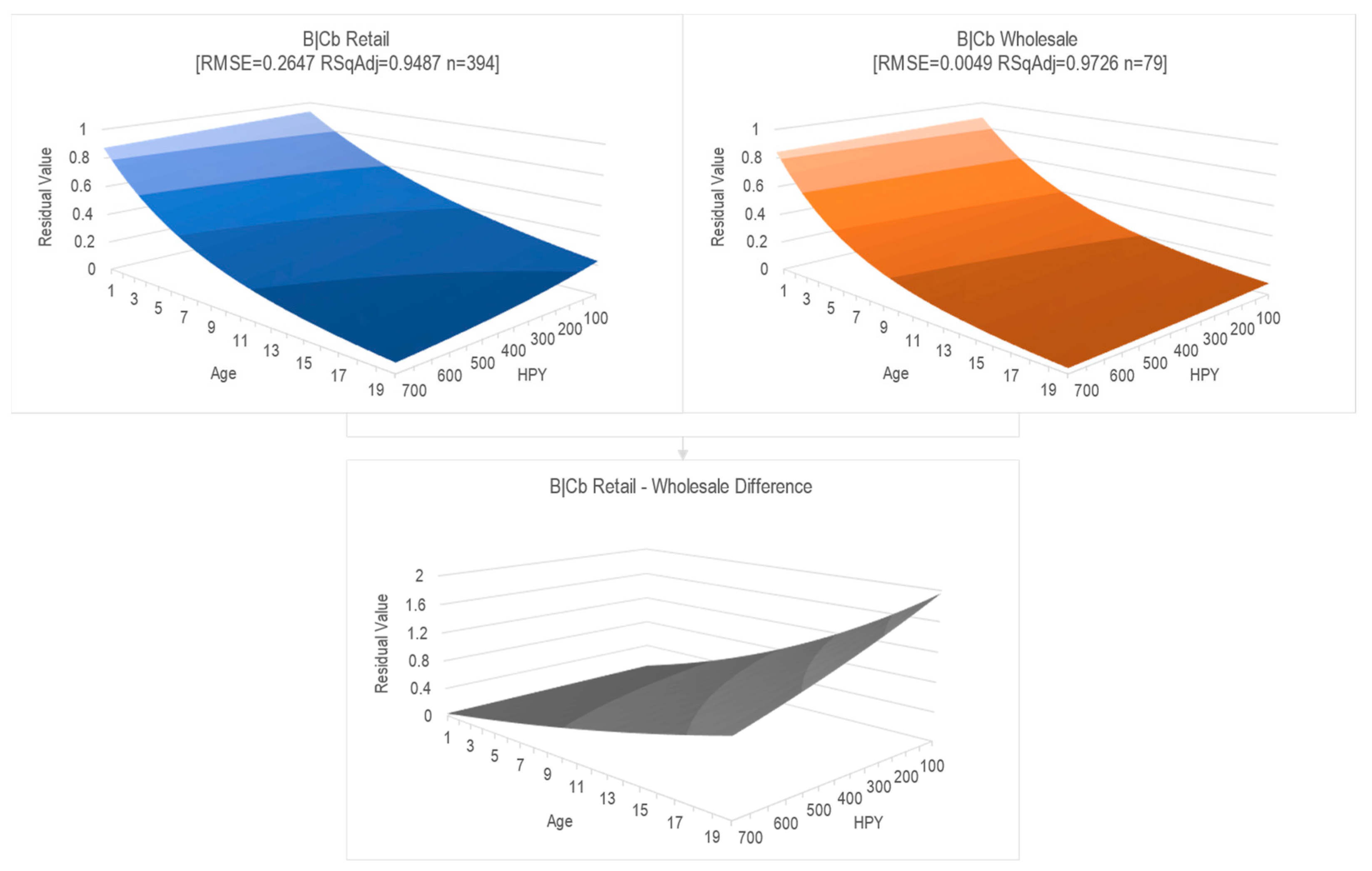
Figure 13.
The proposed power regression model calculated the retail and wholesale residual value of the tractor family B|Cb and calculated the difference.
Figure 13.
The proposed power regression model calculated the retail and wholesale residual value of the tractor family B|Cb and calculated the difference.

Figure 14.
The tractor cohort retail and wholesale residual and their difference and regression.

Figure 15.
The B|Cb tractor cohort retail and wholesale residual value difference regression results of the best-performing regression model.
Figure 15.
The B|Cb tractor cohort retail and wholesale residual value difference regression results of the best-performing regression model.

Figure 16.
The F|Gb and D|E0 tractor cohort retail, wholesale, retail and wholesale residual value difference, and retail and wholesale difference regression results.
Figure 16.
The F|Gb and D|E0 tractor cohort retail, wholesale, retail and wholesale residual value difference, and retail and wholesale difference regression results.


Table 1.
The tractor cohort power regression results.
| Brand Id * | Cohort Id * | RMSE | RSqAdj | Observations |
|---|---|---|---|---|
| A | A|Bb | 0.0094 | 0.9944 | 19 |
| A|Ea | 0.0559 | 0.9488 | 69 | |
| A|Eb | 0.0674 | 0.9682 | 37 | |
| A|Gb | 0.0535 | 0.9784 | 22 | |
| B | B|Cb | 0.0049 | 0.9726 | 79 |
| B|Eb | 0.0337 | 0.9649 | 38 | |
| C | C|Ba | 0.0266 | 0.9835 | 71 |
| C|Ca | 0.0192 | 0.9749 | 35 | |
| C|Da | 0.1004 | 0.9741 | 56 | |
| D | D|C0 | 0.0521 | 0.9756 | 93 |
| D|E0 | 0.0262 | 0.9590 | 31 | |
| D|F0 | 0.0413 | 0.9751 | 113 | |
| D|G0 | 0.0167 | 0.9694 | 31 | |
| E | E|Ba | 0.0196 | 0.9712 | 22 |
| E|Ea | 0.0402 | 0.9745 | 23 | |
| F | F|Eb | 0.0588 | 0.9777 | 52 |
| F|Fb | 0.0470 | 0.9198 | 37 | |
| F|Gb | 0.0175 | 0.9849 | 41 |
* Brand, family, and model are anonymized to avoid any bias.
Table 2.
The fitted regression models with multiple variables and validations for the RMSE results.
| Model Type | Subtype | Analysis | Min RMSE | RSqAdj |
|---|---|---|---|---|
| Ensemble | Boosted trees | 7-predictor hold-out 10% (H|7/0.10) | 0.0632 | 0.8550 |
| Bagged trees | 5 predictors, 5 folds (C|5/5f) | 0.0662 | 0.8383 | |
| Gaussian process regression (GPR) | Exponential GPR | 7-predictor hold-out 10% (H|7/0.10) | 0.0518 | 0.8984 |
| Squared exponential GPR | 7-predictor hold-out 15% (H|7/0.15) | 0.0520 | 0.8753 | |
| Matern 5/2 GPR | 7-predictor hold-out 15% (H|7/0.15) | 0.0521 | 0.8750 | |
| Rational quadratic GPR | 7-predictor hold-out 15% (H|7/0.15) | 0.0523 | 0.8743 | |
| Kernel | SVM kernel | 7-predictor hold-out 15% (H|7/0.15) | 0.0582 | 0.8441 |
| Least-squares regression kernel | 7-predictor hold-out 10% (H|7/0.10) | 0.0583 | 0.8717 | |
| Linear regression | Linear | 7-predictor hold-out 25% (H|7/0.25) | 0.0719 | 0.8077 |
| Robust linear | 7-predictor hold-out 25% (H|7/0.25) | 0.0732 | 0.8006 | |
| Neural network | Narrow neural network | 5 predictors, 3 folds (C|3/5f) | 0.0695 | 0.8222 |
| Medium neural network | 7-predictors hold-out 25% (H|7/0.25) | 0.0834 | 0.7262 | |
| Wide neural network | 7-predictor hold-out 10% (H|7/0.10) | 0.0693 | 0.8185 | |
| Bilayered neural network | 7-predictor hold-out 15% trained 5% (H|7/0.15T0.05) | 0.0725 | 0.6706 | |
| Trilayered neural network | 7-predictor hold-out 15% trained 5% (H|7/0.15T0.05) | 0.0850 | 0.5482 | |
| Stepwise linear regression | Stepwise linear | 7-predictor hold-out 15% (H|7/0.15) | 0.0839 | 0.8545 |
| Support vector machines (SVMs) | Linear SVM | 7 predictors, 5 folds (C|7/5f) | 0.0592 | 0.8385 |
| Quadratic SVM | 5 predictors, 3 folds (C|3/5f) | 0.0621 | 0.8407 | |
| Cubic SVM | 7-predictor hold-out 15% (H|7/0.15) | 0.0945 | 0.6714 | |
| Fine Gaussian SVM | 7-predictor hold-out 15% (H|7/0.15) | 0.0607 | 0.8306 | |
| Medium Gaussian SVM | 7-predictor hold-out 15% (H|7/0.15) | 0.0503 | 0.8834 | |
| Coarse Gaussian SVM | 5 predictors, 5 folds (C|5/5f) | 0.0555 | 0.8579 | |
| Tree | Fine tree | 5 predictors, 3 folds (C|3/5f) | 0.0773 | 0.7799 |
| Medium tree | 7-predictor hold-out 10% (H|7/0.10) | 0.0735 | 0.8011 | |
| Coarse tree | 7-predictor hold-out 10% (H|7/0.10) | 0.0715 | 0.8145 |
Table 3.
The tractor cohort two-predictor regression results.
| Power (Log–Log) Regression | Machine Learning Optimized Gaussian Process Regression | ||||
|---|---|---|---|---|---|
| Tractor Cohort * | RMSE | RSqAdj | RMSE | RSqAdj | Observations |
| A|Bb | 0.0049 | 0.9726 | 0.0533 | 0.7978 | 79 |
| F|Fb | 0.0470 | 0.9198 | 0.0639 | 0.7335 | 37 |
| F|Fa | 0.0192 | 0.9749 | 0.0551 | 0.8892 | 35 |
| A|Ea | 0.0196 | 0.9712 | 0.0490 | 0.8868 | 22 |
| E|Ea | 0.0262 | 0.9590 | 0.0676 | 0.7448 | 31 |
| A|Gb | 0.0266 | 0.9835 | 0.0526 | 0.8534 | 71 |
| F|Ea | 0.0316 | 0.9830 | 0.0624 | 0.8571 | 21 |
| E|Ib | 0.0337 | 0.9649 | 0.0851 | 0.4006 | 38 |
| F|Ib | 0.0361 | 0.9784 | 0.0697 | 0.5990 | 39 |
| F|Gb | 0.0402 | 0.9745 | 0.0572 | 0.6034 | 23 |
* Tractor cohorts are anonymized to avoid any bias.
Table 4.
The retail and wholesale residual value difference regression model results.
| Regression Model | RMSE | RSqAdj |
|---|---|---|
| Linear (lin–lin) | 0.1305 | 0.9813 |
| Logarithmic (lin–log) | 0.3902 | 0.8222 |
| Exponential (log–lin) | 0.3863 | 0.9157 |
| Power (log–log) | 0.3899 | 0.8728 |
| Double square root | 0.0650 | 0.9934 |
| Polynomial 12 | 0.0531 | 0.9957 |
| Polynomial 21 | 0.0770 | 0.9914 |
| Polynomial 22 | 0.0159 | 0.9997 |
Table 5.
Previous study results.
| Researcher | RMSE | RSqAdj | Observations |
|---|---|---|---|
| Cross and Perry (1995) [9] | 1.1061 | 0.7441 | 984 |
| Unterschultz and Mumey (1996) [11] | 5.4442 | 0.5101 | 354 |
| Cross and Perry (1996) [10] | 2.4855 | 0.4661 | 808 |
| Wu and Perry (2004) [12] | 5.8467 | 0.7204 | 984 |
| Fenollosa and Guadalajara (2007) [13] | 6.2488 | 0.6241 | 921 |
| Wilson and Tolley (2004) [14] | 2.0283 | 0.7053 | 984 |
| Wilson (2010) OLS [15] | 11.7206 | 0.6469 | 984 |
| Wilson (2010) Box–Cox [15] | 0.7821 | 0.7441 | 982 |
| ASABE (2011 (R2020)) [16] | 2.2521 | 0.7225 | 984 |
| Kay, Edwards, and Duffy (2020) [17] | 0.0933 | 0.7147 | 624 |
| Witte, Back, Sponagel, and Bahrs (2022) [19] | 0.9306 | 0.4931 | 990 |
| Ruiz-Garcia and Sanchez-Guerrero (2022) [20] | 4.2757 | 0.7580 | 1120 |
Disclaimer/Publisher’s Note: The statements, opinions and data contained in all publications are solely those of the individual author(s) and contributor(s) and not of MDPI and/or the editor(s). MDPI and/or the editor(s) disclaim responsibility for any injury to people or property resulting from any ideas, methods, instructions or products referred to in the content. |
© 2023 by the authors. Licensee MDPI, Basel, Switzerland. This article is an open access article distributed under the terms and conditions of the Creative Commons Attribution (CC BY) license (https://creativecommons.org/licenses/by/4.0/).
Share and Cite
MDPI and ACS Style
Herranz-Matey, I.; Ruiz-Garcia, L. Agricultural Tractor Retail and Wholesale Residual Value Forecasting Model in Western Europe. Agriculture 2023, 13, 2002. https://doi.org/10.3390/agriculture13102002
AMA Style
Herranz-Matey I, Ruiz-Garcia L. Agricultural Tractor Retail and Wholesale Residual Value Forecasting Model in Western Europe. Agriculture. 2023; 13(10):2002. https://doi.org/10.3390/agriculture13102002
Chicago/Turabian StyleHerranz-Matey, Ivan, and Luis Ruiz-Garcia. 2023. "Agricultural Tractor Retail and Wholesale Residual Value Forecasting Model in Western Europe" Agriculture 13, no. 10: 2002. https://doi.org/10.3390/agriculture13102002
Note that from the first issue of 2016, this journal uses article numbers instead of page numbers. See further details here.