
A New Method and Model for the Estimation of Residual Value of Agricultural Tractors

Departamento de Ingeniería Agroforestal, ETSIAAB, Universidad Politécnica de Madrid, Av. Puerta de Hierro, 2, 28040 Madrid, Spain
*
Author to whom correspondence should be addressed.
Agriculture 2023, 13(2), 409; https://doi.org/10.3390/agriculture13020409
Submission received: 31 January 2023
/
Revised: 6 February 2023
/
Accepted: 7 February 2023
/
Published: 9 February 2023
(This article belongs to the Section Agricultural Economics, Policies and Rural Management)
Abstract
:The residual value of a tractor affects the cost of ownership. As there is not much transactional information available for used tractors, nor is there a history of new tractor prices, existing studies struggle to forecast the residual value of agricultural tractors. This is made even more challenging by the emission-regulation-related tractor price increase, low inflation in recent decades, and the complexity of the portfolio offerings from manufacturers. Using the new equivalent tractors, grouped by families of similar characteristics, bypasses these challenges and enables us to obtain larger data sets. These large data sets can be forecasted using transparent linear power regressions that offer the lowest root mean squared error (RMSE = 1.5574) and the highest combined, adjusted coefficient of determination (RSqAdj = 0.8457), outperforming all previously tested studies as well as the ensemble, Gaussian process regression, kernel, linear regression, neural network, support vector machine, and decision tree models. The accessibility of the public information required, as well as its processing using mainstream software through a model that is simple to use, yet robust, enables any stakeholder (manufacturers, sellers, financers, insurers, and, most of all, users) to reliably determine the residual value of an agricultural tractor, empowering them to make fact-based, cost-of-ownership-optimized decisions.
1. Introduction
The operating and ownership costs of machines often comprise more than half of the total crop production costs. Minimizing the machinery portion of the production costs requires a routine assessment of the benefits and costs associated with owning, leasing, or renting machinery [1].
Most farm equipment is still acquired under a conventional purchase plan. The capital may come from the purchaser’s own funds, a third-party lender, or a company financing plan. However, an increasing number of major machinery items are being leased, via operating lease (in which the user can tax-deduct the payments as the machine belongs to the financer), via finance lease (in which the user owns the machine and is therefore entitled to take depreciation deductions) or by using a rollover purchase (in which the operator purchases a new or nearly new piece of equipment from a dealer with the expectation that it will be exchanged for another model after one year or season) [2].
Whether a tractor was paid for upfront, used equipment was traded as a payment in kind, or the machinery was traditionally financed, leased, or rented, the residual value has a tremendous impact on the finance cost, as the financer will ensure that the loan’s lien is below the residual value [3]. If the residual value is uncertain, the financer will include a haircut [4] as a safety factor that renders the finance scheme more expensive to the purchaser.
1.1. Previous Studies
Out of all agricultural machinery, the tractor is a key element in farm/ranch mechanization as most agricultural tasks rely on it, due to its capacity to pull (and push) and take off power (mechanical, hydraulic, and/or electrical) [5]. Therefore, the investment a tractor represents one of the most important investments in both number and value.
Peacock and Brake [6] demonstrated that standard accounting techniques do not adequately reflect the economic deprecation of farm machines. European tax depreciation methods vary tremendously between countries [7], and do not reflect economic depreciation.
Therefore, the importance of a deep understanding of the depreciation rates of agricultural tractors is paramount. Ample research has been conducted on the matter, including the following studies: in the U.S.A., Bradford [8], Musser, Tew, and White [9], Reid and Perry, Bayaner, and Nixon [8], Weersink and Staube [10], Cross and Perry [11,12], Unterschultz and Mumey [13], Dumler, Burton, and Kastens [14,15], Wu and Perry [16], ASABE [17], and Kay, Edwards, and Duffy [18]; in the UK, Williams [19], Cunningham, and Turner, [20], Wilson and Davis [21], Wilson and Tolley [22], and Wilson [23]; in Canada, McNeill [24], Hansen and Lee [25], Witte, Back, Sponagel, and Bahrs [26]; and in Spain, Fenollosa Ribera and Guadalajara Olmeda [27] and Ruiz-Garcia and Sanchez-Guerrero [28].
The depreciation studies defy the challenge by executing regression analyses, which accurately describe the problem as a function of multiple, independent variables. However, different approaches were undertaken by the authors. For example, Wu and Perry [16], ASABE [17], and Kay, Edwards, and Duffy [18] concurred that the independent variables of age, working hours, and engine power have a significant influence on the depreciation; Unterschultz and Mumey [13], Wilson and Tolley [22], Fenollosa Ribera and Guadalajara Olmeda [27], Wilson [23], and Witte, Back, Sponagel, and Bahrs [26] used data that included the tractor manufacturer; and Cross and Perry [11,12] included the care and condition of the tractor as well as additional features or regional influences.
The number of European used tractor sales [29] is small compared to the European passenger car industry [29]. Furthermore, the number of models and, even more so, the substantial number of options, make the statistical sample even more atomized. The difficulty is in accessing a large dataset, which is typically required for empirical studies [23]. In order to address this challenge, some studies, such as Cross and Perry [11,12], Unterschultz and Mumey [13], Dumler, Burton, and Kastens [14,15], Wu and Perry [16], ASABE [17]; Kay, Edwards, and Duffy [18], and Witte, Back, Sponagel, and Bahrs [28], were based on auction prices; others, such as Fenollosa Ribera and Guadalajara Olmeda [27], were based on transactional prices; and still others, such as Wilson and Tolley [22], Wilson [23], and Ruiz-Garcia and Sanchez-Guerrero [28], used advertised prices (Table 1).
1.2. Current Issues
The portfolio offered by manufacturers has grown complex, to the point of offering, with the same engine power, several wheelbases, multiple transmission options and user interfaces, and different shipping and maximum permissible weights with. the same power. These factors have a tremendous impact on selling price (Table 2).
As these features result in different productivity, efficiency, maintenance, and repair requirements they enjoy (or suffer) different demands from the market. Consequently, they have different residual values, despite sharing the same engine power. Thereof, a study considering only the engine power might have challenges discerning the residual value between such different tractors sharing the same power.
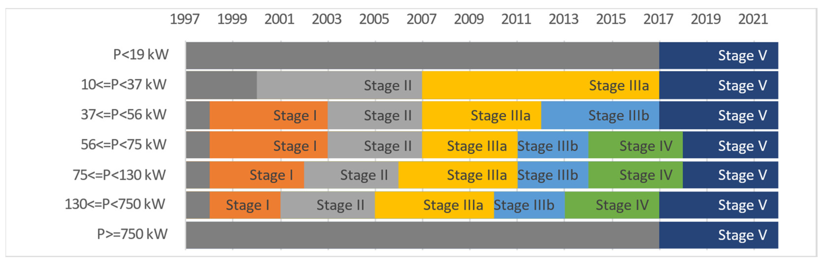
The European Commission (EC) off-road diesel engine emission regulations [30,31,32,33] have had a tremendous impact on the lifespan of tractor series (Figure 1).
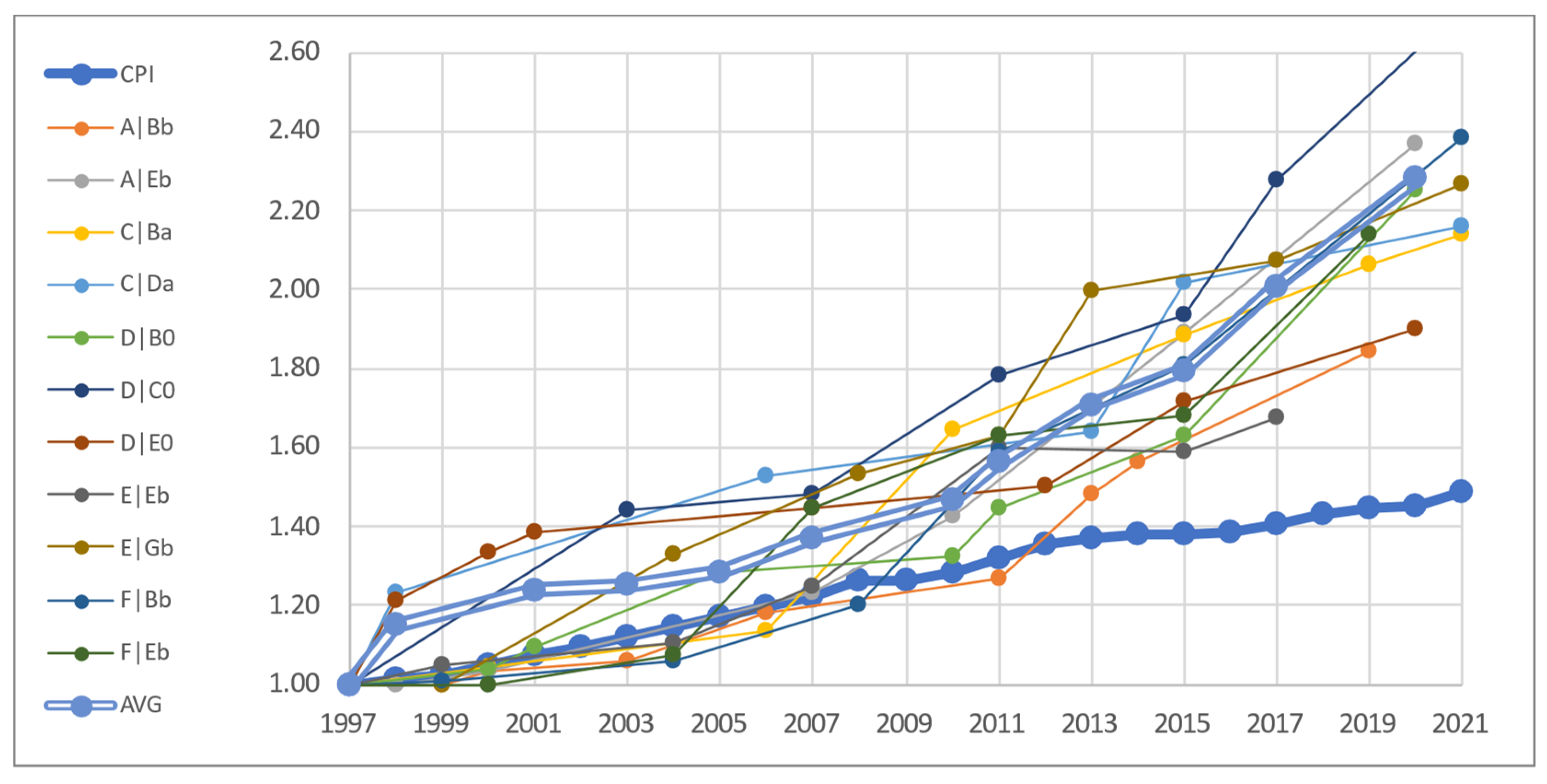
The on-road diesel emission regulations have had an impact on the cost [34,35]. Despite the fact that the last European emission regulation has been already implemented, it is quite likely that new emission regulations will be implemented with their associated costs [36]. The off-road diesel engine emission regulations cost is even higher, as the fixed costs must be distributed amongst a much smaller number of engines (Figure 2).
1.3. Goal
The goal of this research is to develop a residual value calculation methodology that is accessible to all stakeholders (owners, users, marketeers, financiers, and insurers) and that finds a balance between simplicity of use and accurate results. This methodology will be applied to standard, agricultural cabbed tractors with more than 75 kW of horsepower from the main OEMs (Case IH, Claas, Fendt, John Deere, Massey Ferguson, and New Holland) in the main markets of Western Europe [37].
2. Materials and Methods
2.1. Dataset
Transactional European information does not exist in sufficient numbers to be properly analyzed [23]. The number, type, and condition of the European-auctioned machines are not aligned with standard market expectations. Therefore, this study considered agricultural tractors with an engine power higher than 75 kW that were manufactured by Case IH, Claas, Fendt, John Deere, Massey Ferguson, and New Holland and were advertised on https://www.agriaffaires.com/ (accessed on 15 July 2022), https://www.mascus.com/ (accessed on 15 July 2022), and https://www.tractorpool.com/ (accessed on 15 July 2022) by professional retailers (for which the machine is in good condition as the retailer is obliged to provide a legal warranty on the product, and the price realization expectations are delimited by the financial requirements related to their business sustainability) in Austria, Belgium, Denmark, Estonia, Finland, France, Germany, Italy, Latvia, Lithuania, Netherlands, Norway, Poland, Spain, Sweden, and the United Kingdom [37] by professional sellers. The listings needed to feature the working hours, year of manufacture, and price (VAT excluded and price converted into Euros). At least 300 working hours were required, as tractors with less hours advertised from professionals come from demonstration programs or rental programs; hence, there is an outside source of income in which the seller alters the price realization expectations.
The tractor models were aligned with the OEM’s official nomenclature (as sellers tend to include features in the product name with the intent of differentiating their offering), and redundant advertisements were eliminated (as it is frequent that the sellers have business systems interfaced with the different websites in order to achieve the largest possible product awareness; thus, more than one website can feature the same offering).
2.2. Data Systematization and Preprocessing
Calculating the residual value (RV) as:
presents quite a challenge. As mentioned above, the availability of used tractor transactional information is scarce, and obtaining the tractor retail prices from all 16 countries in the scope of this study since 1998 is quite an endeavor. Hence, a novel approach was taken by means of the new equivalent tractor concept:
2.2.1. New Equivalent Tractor
A tractor model belongs to a tractor series, with which it shares a wheelbase, mass, and most characteristics, with the key differentiator being its power. As technology evolves, the tractor series are replaced by newer series with enhancements that improve efficacy and/or efficiency. The evolution is such that it is sometimes not possible to find a current replacement model with the same features as a used one, as those features were rendered obsolete (e.g., synchronized transmissions, two-wheel drive, unsuspended front axle, open circuit hydraulic system, or an open operator station). The retail price of the new series’ models includes any inflation changes as well as any cost derived from regulations compliance and any additional features deemed necessary by the market (Table 4).
Obtaining the retail price of current models will be much easier for the subject matter experts using the method described in this model, as the prices are available through some manufacturer’s websites and/or through a dealer’s quote.
2.2.2. Tractor Family
Manufacturers group their similar models in series. In some cases, these series are quite large and can include several wheelbases, whereas other series are split into separated series (e.g., Case IH’s Puma Series vs. New Holland’s T7 SWB, and T7 LWB or John Deere’s 6 R series, which features models ranging from 6500 kg to 9650 kg of shipping mass). Others differentiate their series by the featured transmission (e.g., Case IH’s CVX, Claas’ CMATIC, Massey Ferguson’s Dyna-VT, and New Holland’s Auto Command series, which features a continuous variable transmission vs. the stepped transmissions featured by equivalent models; Massey Ferguson and New Holland go a step further and differentiate between their models by featuring partial powershift transmissions such as the Dyna-4 and Dyna-6, Electro Command, and Dynamic Command). Other manufacturers use their model nomenclature to differentiate the specifications level (e.g., John Deere’s premium R series vs. the no so premium M series).
In addition, not all series have the same number of sales; thus, the adverts available on the internet are also quite different, allowing for the series to split into different families that share common features and specifications (Table 5).
The combination of the new equivalent tractor and the tractor family have been paramount contributors to coalesce a dataset for this study, which is composed of 10,303 tractors.
2.3. Data Analysis
As previously stated, one of the goals of this study is to provide an easy-to-use method for residual value stakeholders. With 1.1 billion users (one in eight people on the planet), Microsoft Excel is one of the most ubiquitous software in both professional and domestic environments. Hence, considering Microsoft Excel as the first option was clear.
Microsoft Excel offers functions that allow several models to make multiple variable regressions, enabling the evaluation of the following regressions:
In order to evaluate alternative regression options, several different models were analyzed with Matlab, including parametric and non-parametric models (Table 6).
The regression trees, support vector machines, ensembles of regression trees, Gaussian process regressions, and neural networks were optimized by machine learning.
In the interest of examining the predictive accuracy of the fitted models, regressions were made with 3, 5, 7, and 9 predicting variables and with a 3-, 5-, 7-, and 9-fold cross-over validation. In addition, 5%, 10%, 15%, 20%, and 25% hold-out validation models were used (in one instance, one regression was performed with a 5% training dataset) (Table 7).
In regression analysis, the root mean squared error (RMSE) and adjusted R2 (RSqAdj) metrics were used to evaluate the performance of the different models.
The root of the error was used to obtain an error with the same unit as the outcome variable for easier interpretation purposes. The closer the point is to the regression, the lower the metric value is and the higher the accuracy of the regression model is. When a model is 100% perfect, this metric value will be equal to zero.
The adjusted R2 is a better evaluation metric than R2. The R2 is a statistical measure that represents the proportion of variation in the dependent variable that is explained by the regression model. The adjusted R2 considers the number of predictor variables used to predict the dependent variable [38].
As the proposed power regression model is based on tractor families and uses two predictors, the same Matlab regression models seen in Table 6 including regression trees, support vector machines, ensembles of regression trees, Gaussian process regressions, and neural networks optimized by machine learning) were analyzed for the tractor families that obtained the best RMSE results with the proposed power regression model.
3. Results
3.1. Proposed Regression Models
3.2. Fitted Regression Models with Multiple Variables and Validations
Even if one of the goals of this study is to provide the best possible results with the most accessible tools and methodology, it is indispensable to evaluate more advanced models and tools. Therefore, as previously stated, multiple models were evaluated (Table 6) using different variables and validation methods (Table 7).
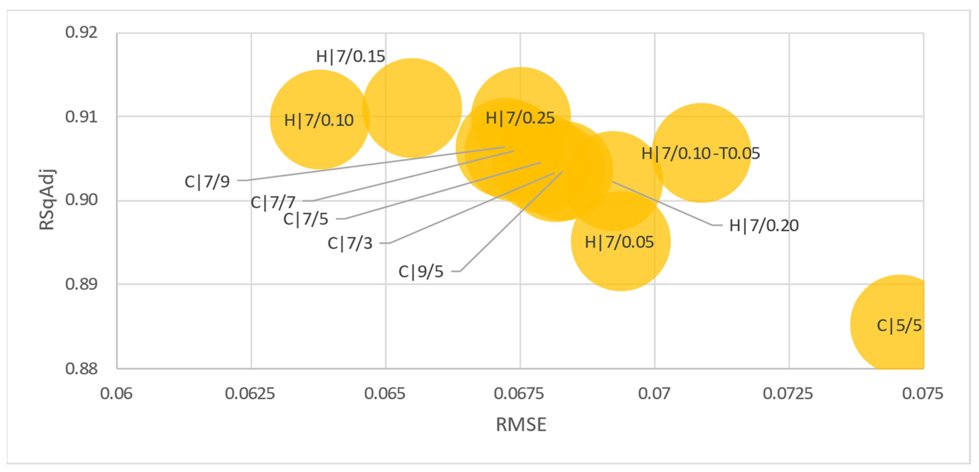
Models with seven predictors showed better RMSE values when compared to 3, 5, and predictor-tested models. Models with hold-out validation demonstrated better RMSE values than those with cross-out validation. The best overall model was the rational quadratic Gaussian process regression with seven predicting variables, which was validated with a 10% hold-out and an RMSE value of 0.046 (Table 9).
This model would rank thirteenth when compared with the tractor families with the best RMSEs of the proposed power model (Table 8).
The exponential Gaussian process regression (GPR) demonstrated more consistent RMSE results across all the tested variables and validations (Figure 5).
3.3. Fitted Regression Models of Tractor Families
As the proposed methodology on power regression models is based on two predicting variables of tractor families, it was essential to test more advanced software using more advanced models.
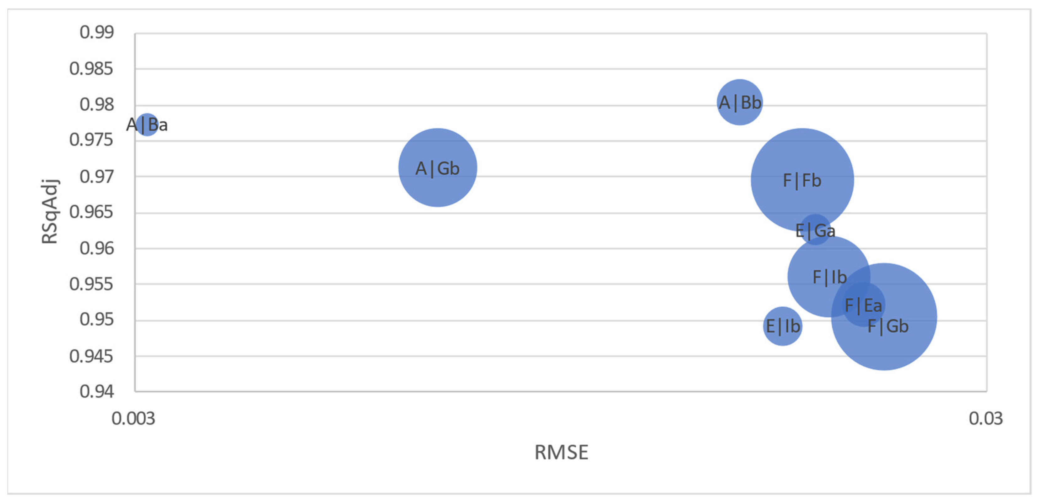
Hence, the tractor families that rendered the best power regression model RMSE value results (Figure 4) were tested using the same fitted models and a 10% hold-out validation to provide data sets (Table 6).
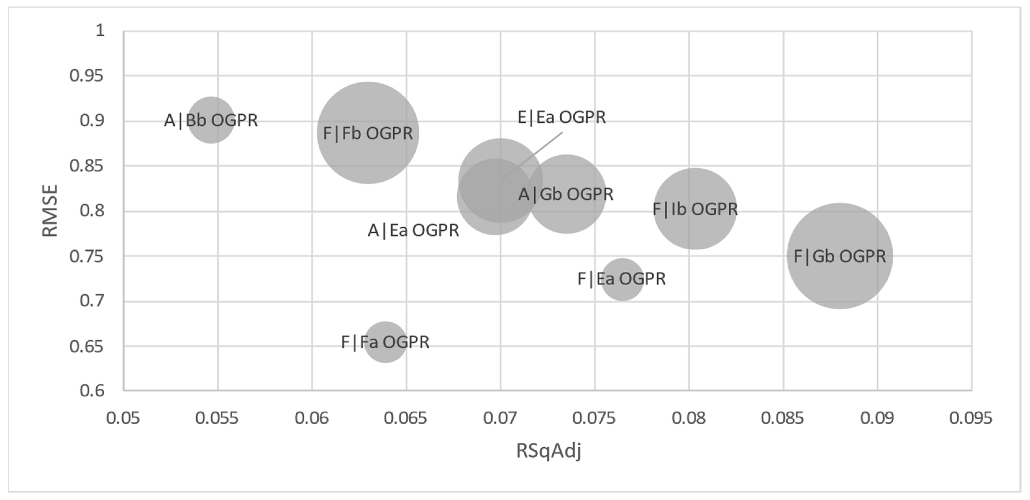
The optimized Gaussian process regressions of the two predictors, validated with a 10% hold-out of the considered tractor families, provided very satisfactory RMSE and RSqAdj results (Table 10).
Across most family groups, the best overall model was the optimized Gaussian process regression (OGPR) model (Figure 6).
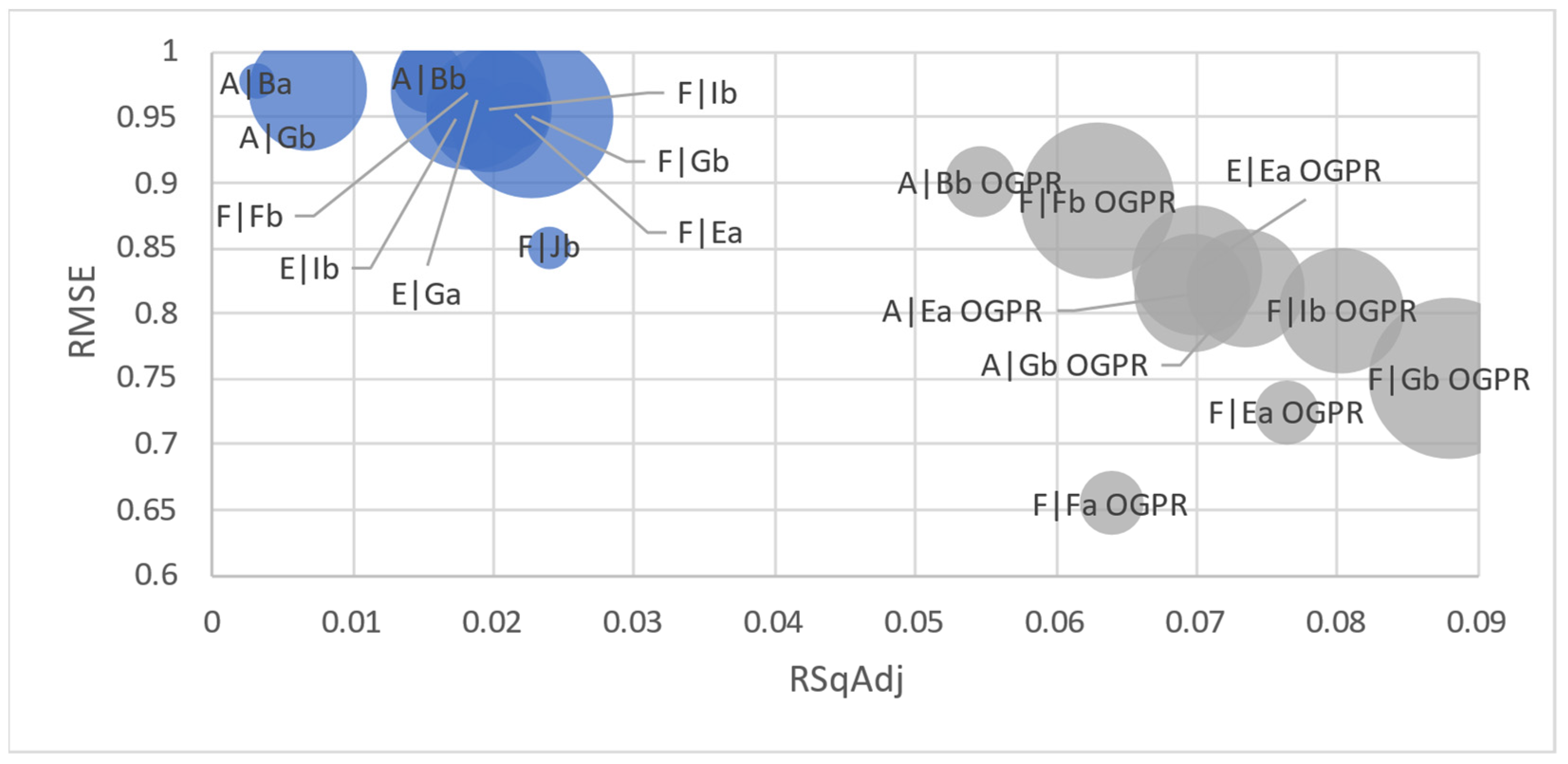
The results of the proposed power regression model of two predictors, grouped by families tested, were better than the most accurate regression performed by Matlab, even if Matlab was optimized by machine learning (Table 11 and Figure 7).
The proposed power regression model seems to follow the different tractor family residual-value behaviors quite precisely. The fact that the second-best tested model was exponential regression, as was found by Witte, Back, Sponagel, and Bahrs [26], proves that these models exhibit better performance than more complex models such as optimized Gaussian regressions (OGPR).
4. Discussion
The robustness of the proposed power regression model was compared to the following models:
4.1. Models Referenced by Previous Studies
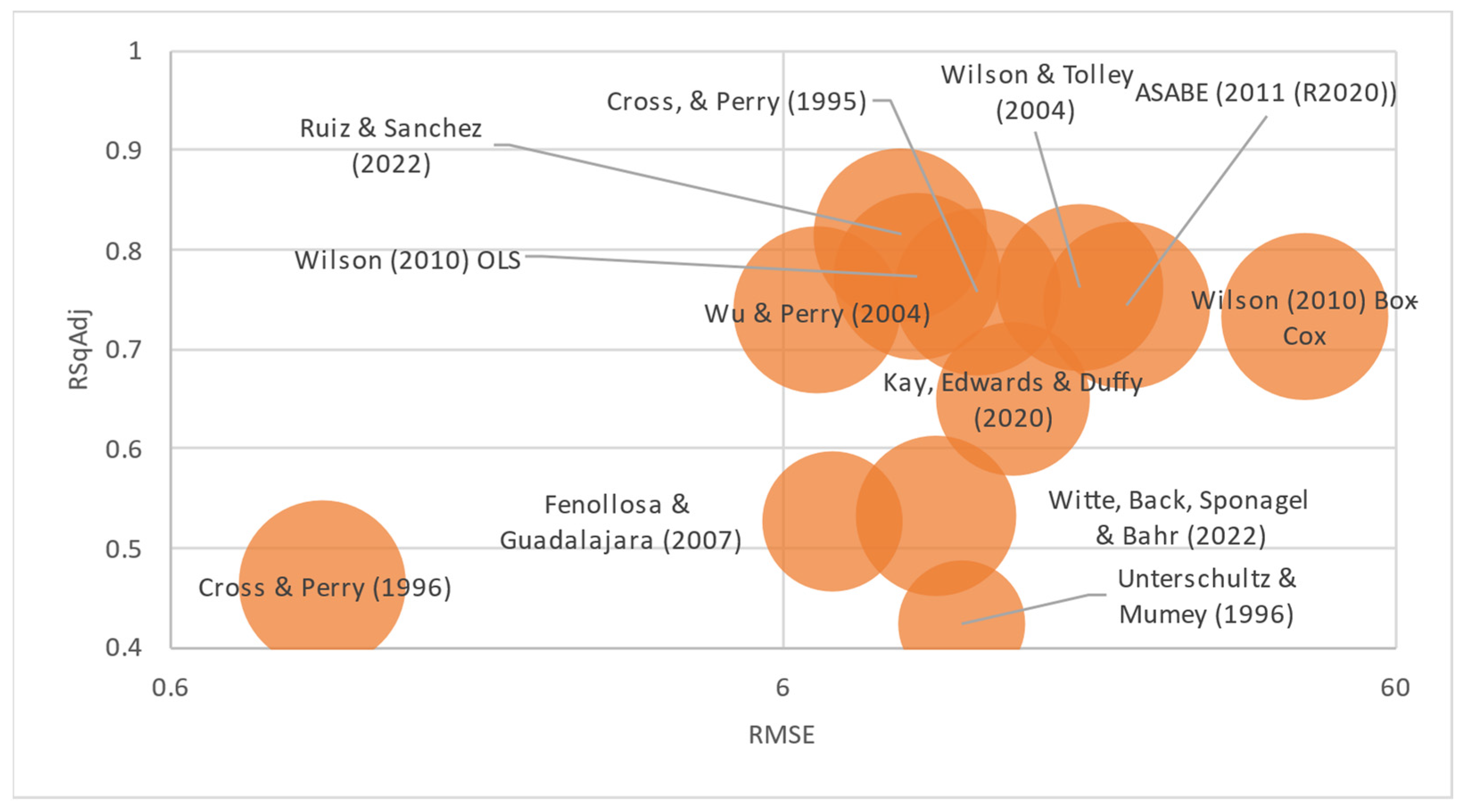
The complete data set was processed using data from previous studies whenever it was possible (when enough details were provided) (Table 12 and Figure 8).
The proposed power regression model (RMSE = 1.5574|RSqAdj = 0.8457) demonstrated more predictive robustness Table 1. shows how previous studies used, in addition to years of age and hours of usage, brand and power in order to predict the residual value behavior. However, Table 2 shows that power is not enough to differentiate residual value behavior, as even similar tractor families from the same brand with the same power can feature different sizes, masses, transmissions, and user interfaces. The proposed model takes these factors into consideration, drilling down to model levels and grouping them in tractor families to lay a better foundation for more robust results.
4.2. General
The proposed power regression model provided the best RMSE and RSqAdj of all the tested models (Figure 9).
Compared to the previous studies referenced, the proposed power regression model provides better RMSE and RSqAdj values as it considers not only the brand and very similar power and tractor size (wheelbase and mass) but also very similar specification levels (e.g., transmissions and user interfaces), relating these factors to an equivalent new model that provides a precise price reference, including inflation and production costs. These variations yield a better foundation for more robust results.
Compared to more advanced fitting models that require specific software, the proposed power regression model provides better RMSE and RSqAdj values and a simpler methodology that is applicable using a more mainstream software.
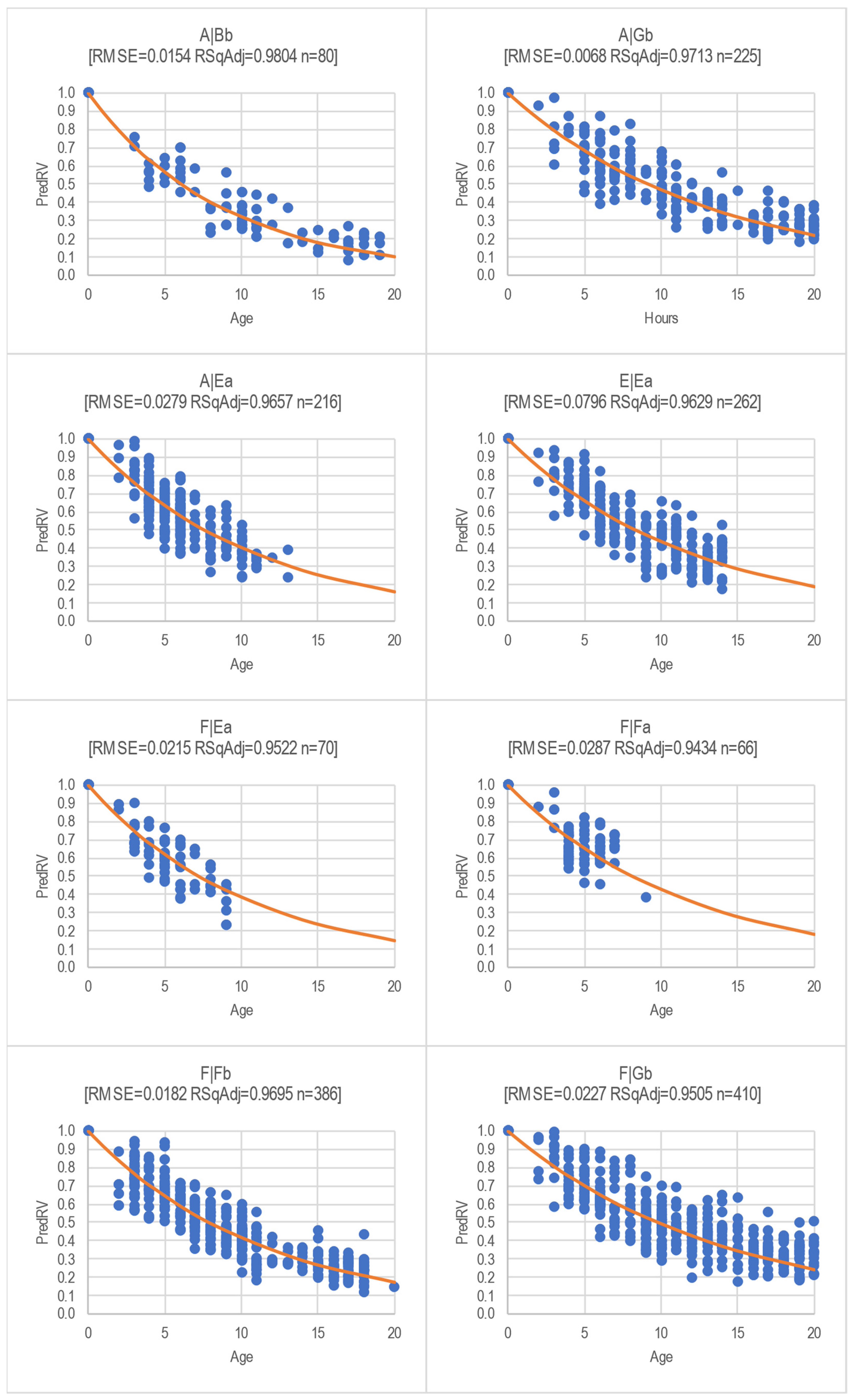
The model is fed from public and freely available data. Its ease of use by means of widely known software, united with its transparency, provides infinite analysis options that can be easily visualized (Figure 10).
The charts created based on the power linear regression model (Figure 10) clearly depict that the more powerful A|Bb tractor family (Table 5) loses value faster than the smaller A|Gb tractor family; both are from the same brand. It also shows how the similar tractor families, A|Ea and E|Ea, and F|Ea, from a different family, which feature similar powers, wheelbases, masses, and stepless transmissions, hold their residual value differently. Additionally, Figure 10 depicts how two very similar tractor families from the same brand, F|Fb and F|Gb, which have a very similar power, wheelbase, mass, and stepped transmission, hold residual value differently.
The methodology and model can be used to compare how the residual value of tractors behaves in tractors with the same power but diverse power densities (kW/kg), transmission options (e.g., continuously variable transmissions, full powershift, and partial powershift transmissions), and user interfaces (from classic to highly advanced).
The methodology can be applied to other types of agricultural machinery, such as combines and self-propelled forage harvesters, as well as to European auction results with similar positive results.
5. Conclusions
This equivalent, new, tractor-based and family-grouped methodology, leading to a power regression curve, solves the issues that affect traditional residual value studies, based on auctions and advertisements, which try to bypass the lack of large transactional datasets. This is true even if the traditional residual value studies take into consideration more predictors (brand, power, economic factors, etc.) than the main drivers (years of age and hours of use) by means of more advanced models (linear, exponential, ordinary least squares, Box–Cox, and robust linear), as can be observed in this study. Simultaneously, the new methodology provides a robust RMSE = 1.5574 and RSqAdj = 0.8457, values which are unsurpassed by all the previous studies and models tested.
The proposed power regression model considers each tractor model on its own. Therefore, there are no interferences from other tractor models with same power but a totally different specification level, wheelbase, and weight.
The proposed power regression model considers the price increase due to emission regulations as well as specification evolution, comparing the used tractor retail price relative to the equivalent new tractor retail price.
The proposed power regression model compensates for the small statistical population by grouping the models in family groups instead of tractor series in cases for which a small statistical population is found, or by subdividing the tractor series when there are sufficient statistical data points and significant differences within tractor series that feature a large number of models.
Despite the simplicity of the proposed power regression model, it was not surpassed by more advanced models (including machine learning optimization) performed by more specialized software.
The proposed power regression model requires a simple internet search for used equipment websites and just two inquiries to sellers (one for the new, equivalent tractor retail price and another inquiry for the used tractor retail price). In other words, it is easy to obtain information that is later transparently processed using a universally known software.
It would be of great interest to identify a way to increase the size of the dataset by including auction results as a source of transactional information if a correlation between retail and wholesale prices is found.
Author Contributions
Conceptualization, I.H.-M.; methodology, I.H.-M. and L.R.-G.; validation, I.H.-M.; formal analysis, I.H.-M. and L.R.-G.; investigation, I.H.-M. and L.R.-G.; resources, I.H.-M.; data curation, I.H.-M.; writing—original draft preparation, I.H.-M. and L.R.-G.; writing—review and editing, I.H.-M. and L.R.-G.; supervision, L.R.-G. All authors have read and agreed to the published version of the manuscript.
Funding
This research received no external funding.
Institutional Review Board Statement
Not applicable.
Informed Consent Statement
Not applicable.
Data Availability Statement
The authors can provide raw data upon request.
Acknowledgments
The authors would like to thank Pilar Linares for her support, and “Tractores y Máquinas” (https://www.tractoresymaquinas.com/) for providing the IT infrastructure for this study.
Conflicts of Interest
The authors declare no conflict of interest.
References
- Kastens, T. Farm Machinery Operations Cost Calculations; Kansas State University, Agricultural Experiment Station and Cooperative Extension Service: Manhattan, KS, USA, 1997. [Google Scholar]
- Edwards, W. Replacement Strategies for Farm Machinery; Iowa State University: Ames, IA, USA, 2019. [Google Scholar]
- U.S. Consumer Financial Protection Bureau. What Is a Loan to Value Ratio and How Does It Relate to My Costs. Available online: https://www.consumerfinance.gov/ask-cfpb/what-is-a-loan-to-value-ratio-and-how-does-it-relate-to-my-costs-en-121/#:~:text=The%20loan%2Dto%2Dvalue%20(,will%20require%20private%20mortgage%20insurance (accessed on 1 January 2023).
- ECB. Haircuts. Available online: https://www.ecb.europa.eu/ecb/educational/explainers/tell-me-more/html/haircuts.en.html (accessed on 1 January 2023).
- Renius, K.T. Fundamentals of Tractor Design; Springer: Cham, Switzerland, 2020. [Google Scholar]
- Peacock, D.L.; Brake, J.R. What Is Used Farm Machinery Worth? Agricultural Experiment Station East Lansing; Department of Agricultural Economics, Michigan State University: East Lansing, MI, USA, 1970. [Google Scholar]
- Veen, H.; Meulen, H.; Bommel, K.; Doorneweert, B. Exploring Agricultural Taxation in Europe; LEI: The Hague, The Netherlands, 2007. [Google Scholar]
- Reid, D.W.; Bradford, G.L. On Optimal Replacement of Farm Tractors. Am. J. Agric. Econ. 1983, 65, 326–331. [Google Scholar] [CrossRef]
- Musser, W.N.; Tew, B.V.; White, F.C. Choice of Depreciation Methods for Farm Firms. Am. J. Agric. Econ. 1986, 68, 980–989. [Google Scholar]
- Weersink, A.; Stauber, S. Optimal Replacement Intercal and Depreciation Method for a Grain Combine. West. J. Agric. Econ. 1988, 13, 18–28. [Google Scholar]
- Cross, T.L.; Perry, G.M. Depreciation Patterns for Agricultural Machinery. Am. J. Agric. Econ. 1995, 77, 194–204. [Google Scholar] [CrossRef]
- Cross, T.; Perry, G. Remaining Value Functions for Farm Equipment. Appl. Eng. Agric. 1996, 12, 547–553. [Google Scholar] [CrossRef]
- Unterschultz, J.; Mumey, G. Reducing Investment Risk in Tractors and Combines with Improved Terminal Asset Value Forecasts. Can. J. Agric. Econ./Rev. Can. D’agroeconomie 1996, 44, 295–309. [Google Scholar]
- Dumler, T.J.; Burton, R.O.; Kastens, T.L. Use of Alternative Depreciation Methods to Estimate Farm Tractor Values. In Proceedings of the Selected Paper at the AAEA Annual Meeting, Tampa, FL, USA, 30 July–2 August 2000; pp. 30–32. [Google Scholar]
- Dumler, T.J.; Burton, R.O.; Kastens, T.L. Predicting Farm Tractor Values through Alternative Depreciation Methods. Rev. Agric. Econ. 2003, 25, 506–522. [Google Scholar]
- Wu, J.; Perry, G.M. Estimating Farm Equipment Depreciation: Which Functional Form Is Best? Am. J. Agric. Econ. 2004, 86, 483–491. [Google Scholar] [CrossRef]
- ASAE Standard D497.7; ASABE Agricultural Machinery Management Data. American Society of Agricultural and Biological Engineers: Joseph, MI, USA, 2020.
- Kay, R.D.; Edwards, W.M.; Duffy, P.A. Farm Management, 7th ed.; McGraw-Hill: New York, NY, USA, 2020. [Google Scholar]
- Williams, N.T. Appropriate Rates of Depreciation for Machinery in Current Cost Accounting. Farm Manag. 1981, 4, 171–176. [Google Scholar]
- Cunningham, S.; Turner, M.M. Actual Depreciation Rates of Farm Machinery. Farm Manag. 1988, 6, 381–387. [Google Scholar]
- Wilson, P.; Davis, S. Estimating Depreciation in Tractors in the UK and Implications for Farm Management Decision Making. Farm Manag. 1998, 10, 183–193. [Google Scholar]
- Wilson, P.; Tolley, C. Estimating Tractor Depreciation and Implications for Farm Management Accounting. J. Farm Manag. 2004, 12, 5–16. [Google Scholar]
- Wilson, P. Estimating Tractor Depreciation: The Impact of Choice of Functional Form. J. Farm Manag. 2010, 13, 799–818. [Google Scholar]
- McNeill, R.C. Depreciation of Farm Tractors in British Columbia. Can. J. Agric. Econ./Rev. Can. D’agroeconomie 1979, 27, 53–58. [Google Scholar] [CrossRef]
- Hansen, L.; Lee, H. Estimating Farm Tractor Depreciation: Tax Implications. Can. J. Agric. Econ./Rev. Can. D’agroeconomie 1991, 39, 463–479. [Google Scholar] [CrossRef]
- Witte, F.; Back, H.; Sponagel, C.; Bahrs, E. Remaining Value Development of Tractors—A Call for the Application of a Differentiated Market Value Estimation. Agric. Eng. 2022, 77, 1–20. [Google Scholar] [CrossRef]
- Fenollosa, M.; Guadalajara, N. An Empirical Depreciation Model for Agricultural Tractors in Spain. Span. J. Agric. Res. 2007, 5, 130–141. [Google Scholar] [CrossRef]
- Ruiz-Garcia, L.; Sanchez-Guerrero, P. A Decision Support Tool for Buying Farm Tractors, Based on Predictive Analytics. Agriculture 2022, 12, 331. [Google Scholar] [CrossRef]
- ACEA. Economic and Market Report. State of the EU Auto Industry. Full-Year 2021; European Automobile Manufacturers’ Association (ACEA): Brussels, Belgium, 2022. [Google Scholar]
- EC. Directive 97/68/EC of the European Parliament and of the Council of 16 December 1997; European Commission (EC): Brussels, Belgium, 1997.
- EC. Directive 2000/25/EC of the European Parliament; European Commission (EC): Brussels, Belgium, 2000.
- EC. Directive 2004/26/EC of the European Parliament and of the Council of 21 April 2004 Amending Directive 97/68/EC; European Commission (EC): Brussels, Belgium, 2004.
- EC. Directive 2009/30/EC of the European Parliament and of the Council of 23 April 2009 Amending Directive 98/70/EC; European Commission (EC): Brussels, Belgium, 2009.
- Posada, F.; Chambliss, S.; Blumberg, K. Cost of Emission Reduction Technologies for Heavy Duty Diesel Vehicles; The International Council on Clean Transportation: Washington, DC, USA, 2016. [Google Scholar]
- Lynch, L.A.; Hunter, C.A.; Zigler, B.T.; Thomton, M.J.; Reznicek, E.P. On-Road Heavy-Duty Low-NOx Technology Cost Study; National Renewable Energy Laboratory (NREL), U.S. Department of Energy: Golden, CO, USA, 2020.
- Posada, F.; Isenstadt, A.; Badshah, H. Estimated Cost of a Diesel Emissions-Control Technology to Meet Future California Low NOx Standards in 2024 and 2027; The International Council of Clean Transportation: Washington, DC, USA, 2020. [Google Scholar]
- CEMA. Economic Press Release Tractor Registrations 2021; CEMA—European Agricultural Machinery: Brussels, Belgium, 2022. [Google Scholar]
- McCarthy, R.V.; McCarthy, M.M.; Ceccucci, W.; Halawi, L. Applying Predictive Analytics; Springer International Publishing: Cham, Switzerland, 2019. [Google Scholar]
Figure 1.
European off-road diesel engine emission regulations implementation by engine power.

Figure 2.
Eurozone harmonized index of consumer prices (HICP) and Germany’s tractor family MSRP evolution relative to 1997.
Figure 2.
Eurozone harmonized index of consumer prices (HICP) and Germany’s tractor family MSRP evolution relative to 1997.

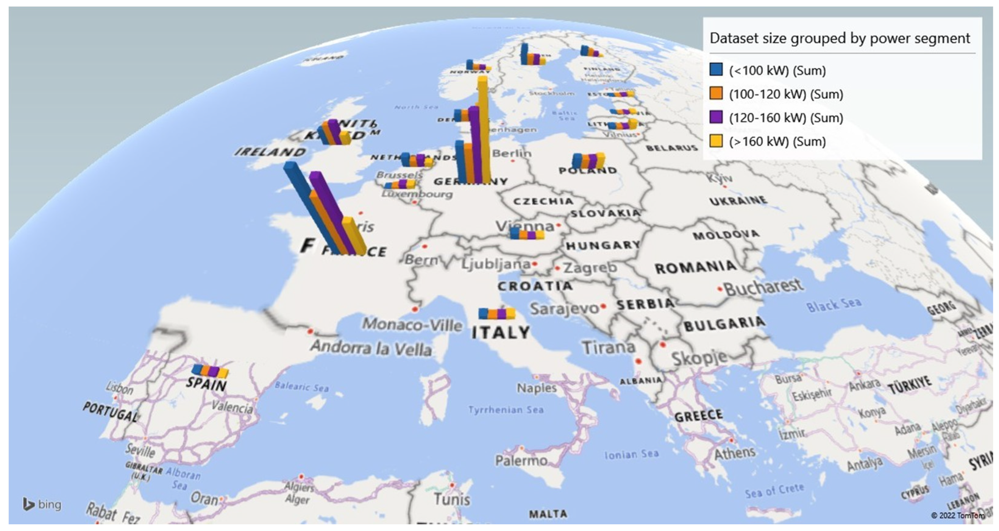
Figure 3.
Dataset size grouped by country and power segment.

Figure 4.
Power regression results (bubble size represents number of observations).

Figure 5.
Exponential Gaussian process (GPR) results’ RMSE for different tested variables and validations (bubble size represents number of observations).
Figure 5.
Exponential Gaussian process (GPR) results’ RMSE for different tested variables and validations (bubble size represents number of observations).

Figure 6.
RMSE values for optimized Gaussian process results of two predictors, grouped by families tested (bubble size represents number of observations).
Figure 6.
RMSE values for optimized Gaussian process results of two predictors, grouped by families tested (bubble size represents number of observations).

Figure 7.
Two predictors, grouped by family power regression (blues) and OGPR (grey) results (bubble size represents number of observations).
Figure 7.
Two predictors, grouped by family power regression (blues) and OGPR (grey) results (bubble size represents number of observations).

Figure 8.
Reults of previously referenced studies (bubble size represents number of observations).

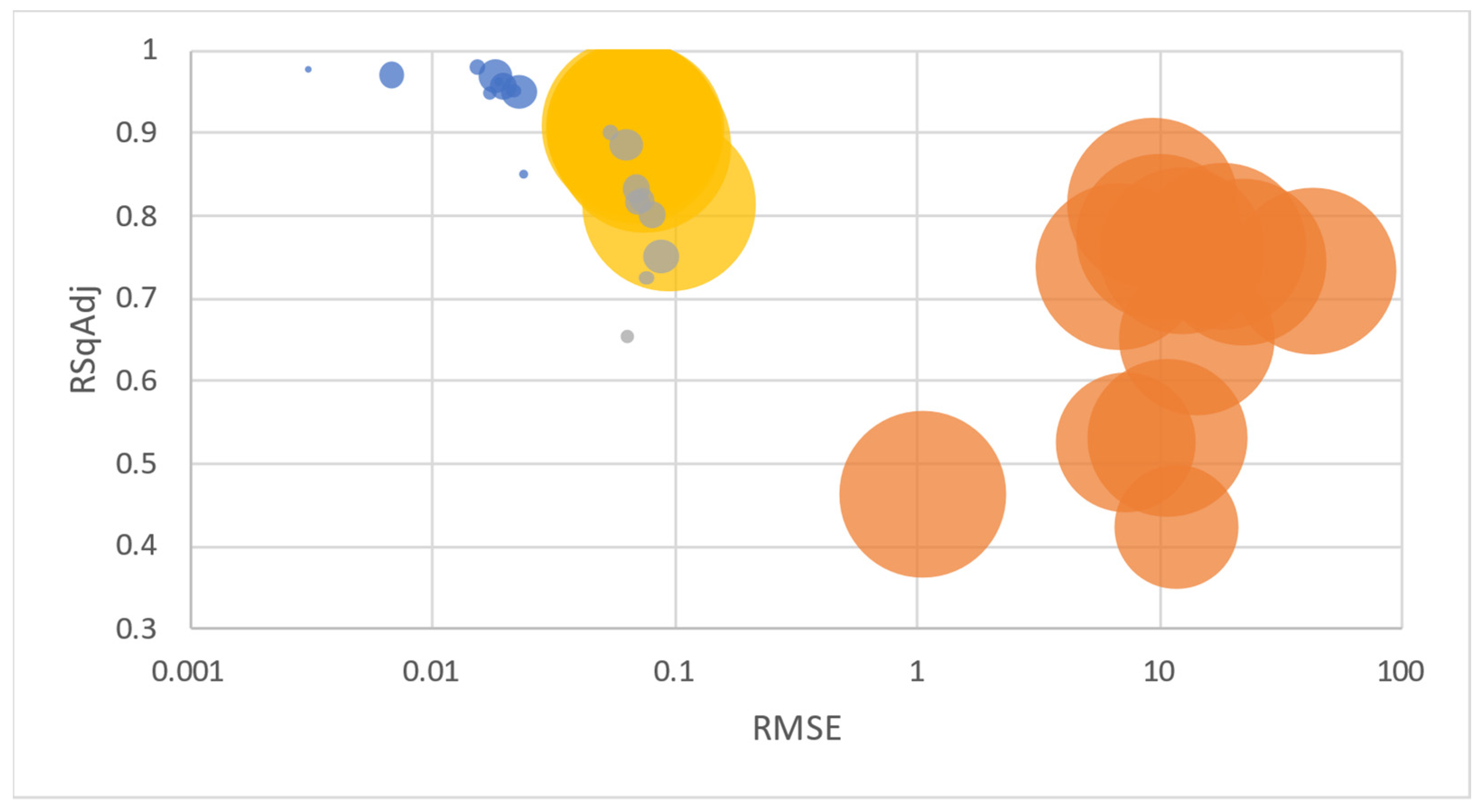
Figure 9.
Summary of all regressions considered in this study (proposed power regression in blue, previous studies referenced in orange, fitted multiple variables and validation models in yellow, and fitted tractor family models in gray) (bubble size represents number of observations).
Figure 9.
Summary of all regressions considered in this study (proposed power regression in blue, previous studies referenced in orange, fitted multiple variables and validation models in yellow, and fitted tractor family models in gray) (bubble size represents number of observations).

Figure 10.
Dataset and power regression for 500 h per year (HPY) results of top eight RMSE tractor families.
Figure 10.
Dataset and power regression for 500 h per year (HPY) results of top eight RMSE tractor families.


Table 1.
Details of previous studies.
| Reference | Data Source | Data Size | Variables | Function |
|---|---|---|---|---|
| Peacock, D. L., and Brake, J. R. (1970). | U.S.A. Sales | - | Age | Linear |
| ASAE (1979). | U.S.A. | - | Age | Exponential |
| McNeill, R. C. (1979). | Canada | 32 | Age and state | Exponential |
| Leatham, D. J., and Baker, T. G. (1981). | U.S.A. | 1454 tractors | Age, power, motor type, traction, and manufacturer | Exponential |
| Reid, D. W., and Bradford, G. L. (1983). | U.S.A. | 411 | Age, power, motor type, manufacturer, increasing usage, and technological changes | Exponential |
| Perry, G. M., Bayaner, A., and Nixon, C. J. (1986). | U.S.A. | 1612 | Age, power, manufacturer, usage, care, and macroeconomic variables | Box–Cox |
| Hansen, L., and Lee, H. (1991). | Canada | - | Age, year of manufacture, and purchase year | Linear |
| Cross, T. L., and Perry, G. M. (1995). | U.S.A. Auctions | - | Age, usage, manufacturer, care, type of auction, region, and macroeconomic variables | Box–Cox |
| Unterschultz, J., and Mumey, G. (1996). | U.S.A. and Canadian Auctions | 3202 Tractors | Age, manufacturer | Ratified by Hansen and Lee model |
| Cross, T. L., and Perry, G. M. (1996). | U.S.A. Auctions | 433 <60 kW 1946 60–112 kW 866 >112 kW | Age, usage, manufacturer, care, and macroeconomic variables | Box–Cox |
| Wu, J., and Perry, G. M. (2004). | U.S.A. Auctions | 657 30–79 hp 1420 80–120 hp 781 121+ hp | Age, production year, manufacturer, and other | Box–Cox |
| Fenollosa Ribera, M. L., and Guadalajara Olmeda, N. (2007). | E.S. Sales | 7876 13–79 hp 3963 80–133 hp 731 134–263 hp Dec’99-Dec’02 | Age, power, brand, and others | Ordinary Least Squares (OLS) |
| Wilson, P., and Tolley, C. (2004). | U.K. Adverts | 968 | Age, hours, power, brand, and others | Ordinary Least Squares (OLS) |
| Wilson, P. (2010). | U.K. Adverts | 1223 | Age, hours, power, brand, and others | Ordinary Least Squares (OLS) Box–Cox |
| ASABE. (2011 (R2020)). | U.S.A. | - | Age, usage, and power | Box–Cox |
| Kay, R. D., Edwards, W. M., and Duffy, P. A. (2020). | U.S.A. Auctions. | - | Based on ASABE standards, 2006 | Box–Cox |
| Witte, F., Back, H., Sponagel, C., and Bahrs, E. (2022) | German Adverts and Auctions | 2667 tractors | Age, hours, power, and brand | Exponential |
| Ruiz-Garcia, L., and Sanchez-Guerrero, P. (2022). | EUR Adverts | 227 new 1003 used | Age, hours, power, and brand | Robust linear (polynomic) |
Table 2.
Manufacturer’s suggested retail price (MSRP) for 107 kW from one brand relative to the most economical offering.
Table 2.
Manufacturer’s suggested retail price (MSRP) for 107 kW from one brand relative to the most economical offering.
| Model Identifier | B|Hb|006 * | B|Gb|005 * | B|Ga|005 * | B|Eb|001 * | B|Ea|001 * |
|---|---|---|---|---|---|
| Rated Power | 107 kW | ||||
| Wheelbase | 2525 mm | 2564 mm | 2820 mm | ||
| Shipping Mass | 5300 kg | 6940 kg | 7470 kg | ||
| Max Mass | 9000 kg | 10,250 kg | 10,250 kg | ||
| Transmission | Partial Powershift Transmission | Partial Powershift Transmission | Continuous Variable Transmission | Partial Powershift Transmission | Continuous Variable Transmission |
| MSRP relative to the most economical offering | |||||
| Classic Interface | 1.00 | ||||
| Advanced Interface | 1.05 | 1.13 | 1.11 | ||
| Premium Interface | 1.14 | 1.17 | 1.28 | 1.16 | 1.34 |
| Ultimate Interface | 1.22 | 1.33 | 1.21 | 1.39 | |
* Brand, family, and model are anonymized to avoid any bias.
Table 3.
Dataset size grouped by country and power segment.
| Country | (<100 kW) | (100–120 kW) | (120–160 kW) | (>160 kW) | Total |
|---|---|---|---|---|---|
| Austria | 77 | 28 | 19 | 32 | 156 |
| Belgium | 12 | 24 | 59 | 52 | 147 |
| Denmark | 105 | 92 | 126 | 183 | 506 |
| Estonia | 7 | 9 | 20 | 38 | 74 |
| Finland | 117 | 83 | 58 | 15 | 273 |
| France | 1097 | 773 | 992 | 444 | 3306 |
| Germany | 459 | 420 | 838 | 1132 | 2849 |
| Italy | 65 | 35 | 39 | 66 | 205 |
| Latvia | 7 | 6 | 7 | 22 | 42 |
| Lithuania | 34 | 24 | 25 | 85 | 168 |
| Netherlands | 117 | 68 | 105 | 54 | 344 |
| Norway | 93 | 39 | 37 | 4 | 173 |
| Poland | 134 | 114 | 115 | 138 | 501 |
| Spain | 60 | 43 | 48 | 22 | 173 |
| Sweden | 246 | 116 | 119 | 70 | 551 |
| United Kingdom | 192 | 246 | 273 | 124 | 835 |
| Total | 2822 | 2120 | 2880 | 2481 | 10,303 |
Table 4.
Model evolution example.
| Model | Year | Power | Wheelbase | Minimum Mass | Transmission Options |
|---|---|---|---|---|---|
| Current Model | 2022–2020 | 186 kW | 2925 mm | 11,400 kg | Infinitely variable transmission, 23-speed full powershift |
| Predecessor-1 | 2020–2014 | 186 kW | 2925 mm | 10,470 kg | Infinitely variable transmission, 23-speed full powershift |
| Predecessor-2 | 2014–2012 | 172 kW | 2925 mm | 10,285 kg | Infinitely variable transmission, 23-speed full powershift |
| Predecessor-3 | 2012–2006 | 173 kW | 2860 mm | 7900 kg | Infinitely variable transmission, 19-speed full powershift, 20-speed partial powershift, 16-speed partial powershift, |
| Predecessor-4 | 2006–2003 | 141 kW | 2860 mm | 7772 kg | Infinitely variable transmission, 19-speed full powershift, 20-speed partial powershift |
| Predecessor-5 | 2003–1996 | 130 kW | 2800 mm | 6510 kg | Infinitely variable transmission, 19-speed full powershift, 20-speed partial powershift |
| Predecessor-6 | 1996–1992 | 127 kW | 2800 mm | 6495 kg | 19-speed full powershift, 16-speed partial powershift |
| Predecessor-7 | 1992–1988 | 117 kW | 2670 mm | 6400 kg | 15-speed full powershift, 16-speed partial powershift |
| Predecessor-8 | 1998–1983 | 117 kW | 2670 mm | 5790 kg | 15-speed full powershift, 16-speed partial powershift |
| Predecessor-9 | 1982–1978 | 107 kW | 2710 mm * | 5300 kg | 8-speed full powershift, 16-speed partial powershift |
| Predecessor-10 | 1978–1973 | 102 kW | 2700 mm * | 4415 kg | 8-speed full powershift, 16-speed partial powershift, 8-speed partially synchro |
| Predecessor-11 | 1972–1971 | 95 kW | 2700 mm * | 4105 kg | 8-speed full powershift, 8-speed partially synchro |
* Two-wheel drive (2 WD).
Table 5.
Family model details.
| Brand Id * | Family Id * | Number of Models | Min Power (kW) | Max Power (kW) | Wheelbase (mm) | Minimum Mass (kg) | Maximum Mass (kg) |
|---|---|---|---|---|---|---|---|
| A | A|Ba | 5 | 184 | 279 | 3155 | 11,290 | 18,000 |
| A|Bb | 5 | 184 | 250 | 3155 | 11,290 | 18,000 | |
| A|Ca | 3 | 184 | 221 | 2995 | 10,500 | 16,000 | |
| A|Ea | 7 | 110 | 177 | 2884 | 6782 | 13,000 | |
| A|Eb | 5 | 110 | 162 | 2884 | 6782 | 13,000 | |
| A|Ga | 4 | 92 | 107 | 2679 | 5300 | 9500 | |
| A|Gb | 5 | 85 | 107 | 2454 | 5190 | 9000 | |
| A|Ib | 3 | 73 | 84 | 2420 | 4390 | 8000 | |
| A|Jb | 7 | 43 | 84 | 2235 | 2880 | 6000 | |
| B | B|Ba | 4 | 232 | 298 | 3150 | 12,840 | 18,000 |
| B|Ca | 7 | 142 | 195 | 2980 | 8300 | 14,000 | |
| B|Cb | 7 | 142 | 195 | 2980 | 8300 | 14,000 | |
| B|Ea | 4 | 110 | 129 | 2820 | 6570 | 12,000 | |
| B|Eb | 4 | 110 | 129 | 2820 | 6570 | 12,000 | |
| B|Ga | 3 | 103 | 116 | 2564 | 5800 | 11,000 | |
| B|Gb | 3 | 103 | 116 | 2564 | 5800 | 11,000 | |
| B|Hb | 6 | 63 | 99 | 2525 | 4700 | 8500 | |
| C | C|Aa | 4 | 291 | 380 | 3300 | 14,000 | 18,000 |
| C|Ba | 5 | 202 | 291 | 3050 | 10,830 | 18,000 | |
| C|Ca | 4 | 166 | 211 | 2950 | 9370 | 16,000 | |
| C|Da | 6 | 106 | 176 | 2783 | 7735 | 14,000 | |
| C|Ga | 4 | 91 | 120 | 2560 | 6050 | 10,500 | |
| C|Ha | 4 | 74 | 97 | 2420 | 4810 | 8500 | |
| D | D|B0 | 7 | 180 | 294 | 3050 | 13,528 | 18,000 |
| D|C0 | 6 | 154.5 | 228 | 2925 | 10,470 | 16,000 | |
| D|E0 | 3 | 129 | 158 | 2183 | 8300 | 13,450 | |
| D|E1 | 2 | 126 | 143 | 2800 | 7015 | 12,300 | |
| D|F0 | 3 | 99 | 114 | 2765 | 6400 | 11,750 | |
| D|F1 | 3 | 107 | 114 | 2765 | 6700 | 11,000 | |
| D|G0 | 3 | 81 | 96 | 2580 | 6000 | 9950 | |
| D|G1 | 3 | 96 | 103 | 2580 | 5800 | 10,450 | |
| D|H1 | 6 | 66 | 88 | 2400 | 5750 | 10,450 | |
| D|I0 | 4 | 66.6 | 91.9 | 2250 | 4300 | 8600 | |
| D|I1 | 4 | 55 | 85 | 2300 | 3600 | 6000 | |
| E | E|Ba | 5 | 176 | 250 | 3093 | 10,800 | 18,000 |
| E|Ea | 8 | 106 | 173 | 3000 | 5800 | 13,000 | |
| E|Eb | 9 | 101 | 176 | 3000 | 5800 | 13,000 | |
| E|Ec | 2 | 101 | 106 | 2880 | 5800 | 12,500 | |
| E|Ga | 6 | 88 | 129 | 2870 | 5500 | 11,500 | |
| E|Gb | 6 | 88 | 129 | 2670 | 5500 | 11,500 | |
| E|Gc | 4 | 88 | 110 | 2670 | 5500 | 8800 | |
| E|Hb | 3 | 82 | 97 | 2550 | 4800 | 8421 | |
| E|Hc | 5 | 70 | 97 | 2550 | 4800 | 8421 | |
| F | F|Ba | 5 | 184 | 279 | 3500 | 11,235 | 18,000 |
| F|Bb | 5 | 184 | 279 | 3500 | 11,235 | 18,000 | |
| F|Ca | 3 | 184 | 221 | 2995 | 10,500 | 16,000 | |
| F|Ea | 4 | 132 | 177 | 2884 | 8140 | 13,000 | |
| F|Eb | 4 | 132 | 177 | 2884 | 8140 | 13,000 | |
| F|Fa | 4 | 103 | 132 | 2789 | 6650 | 11,500 | |
| F|Fb | 4 | 103 | 132 | 2789 | 6650 | 11,500 | |
| F|Ga | 4 | 85 | 107 | 2684 | 6360 | 10,500 | |
| F|Gb | 6 | 85 | 107 | 2684 | 6110 | 10,500 | |
| F|Ib | 3 | 74 | 86 | 2380 | 5300 | 8000 | |
| F|Jb | 5 | 55 | 84 | 2285 | 3700 | 6500 |
* Brand, family and model are anonymized to avoid any bias.
Table 6.
Tested fitted regression models.
| Model Type | Subtype |
|---|---|
| Ensemble | Bagged Trees |
| Boosted Trees | |
| Gaussian Process Regression (GPR) | Exponential GPR |
| Matern 5/2 GPR | |
| Rational Quadratic GPR | |
| Squared Exponential GPR | |
| Kernel | Least Squares Regression Kernel |
| SVM Kernel | |
| Linear Regression | Linear |
| Robust Linear | |
| Neural Network | Bi-layered Neural Network |
| Medium Neural Network | |
| Narrow Neural Network | |
| Tri-layered Neural Network | |
| Wide Neural Network | |
| Supported Vector Machine (SVM) | Coarse Gaussian SVM |
| Cubic SVM | |
| Fine Gaussian SVM | |
| Linear SVM | |
| Medium Gaussian SVM | |
| Quadratic SVM | |
| Tree | Coarse Tree |
| Fine Tree | |
| Medium Tree |
Table 7.
Number of predicting variables and validations evaluated.
| Predictor Variables | Validation | |||||||||
|---|---|---|---|---|---|---|---|---|---|---|
| Cross-Over | Hold-Out | |||||||||
| 3 Folds | 5 Folds | 7 Folds | 9 Folds | 5% | 10% | 10% (T5%) | 15% | 20% | 25% | |
| 3 | + | |||||||||
| 5 | + | |||||||||
| 7 | + | + | + | + | + | + | + | + | + | + |
| 9 | + | |||||||||
Table 8.
Tractor family power regression results.
| Brand Identifier | Family Identifier | RMSE | RSqAdj | Observations |
|---|---|---|---|---|
| A | A|Ba | 0.0031 | 0.9773 | 20 |
| A|Bb | 0.0154 | 0.9804 | 80 | |
| A|Ea | 0.0279 | 0.9657 | 216 | |
| A|Eb | 0.1039 | 0.9664 | 212 | |
| A|Gb | 0.0068 | 0.9713 | 225 | |
| A|Ib | 0.1989 | 0.9381 | 66 | |
| B | B|Cb | 0.2647 | 0.9487 | 394 |
| B|Eb | 0.3786 | 0.9479 | 536 | |
| B|Gb | 0.0856 | 0.8549 | 64 | |
| B|Hb | 0.3879 | 0.9202 | 215 | |
| C | C|Ba | 0.4028 | 0.9642 | 388 |
| C|Ca | 0.3890 | 0.9608 | 266 | |
| C|Da | 0.8513 | 0.9713 | 502 | |
| C|Ga | 0.1674 | 0.9497 | 160 | |
| C|Ha | 0.0842 | 0.9446 | 36 | |
| D | D|B0 | 0.2124 | 0.9742 | 291 |
| D|C0 | 0.1868 | 0.9753 | 613 | |
| D|E0 | 0.3358 | 0.9579 | 727 | |
| D|F0 | 0.7231 | 0.9594 | 907 | |
| D|F1 | 0.2544 | 0.8969 | 162 | |
| D|G0 | 0.7570 | 0.9311 | 466 | |
| D|G1 | 0.5214 | 0.8146 | 306 | |
| D|H1 | 0.6589 | 0.9061 | 93 | |
| D|I0 | 0.1239 | 0.9301 | 83 | |
| D|I1 | 0.2733 | 0.3018 | 51 | |
| E | E|Ba | 0.2578 | 0.9763 | 88 |
| E|Ea | 0.0796 | 0.9629 | 262 | |
| E|Eb | 0.1099 | 0.9697 | 338 | |
| E|Ga | 0.0189 | 0.9626 | 36 | |
| E|Gb | 0.6431 | 0.9258 | 495 | |
| E|Gc | 0.0849 | 0.9783 | 36 | |
| E|Hb | 0.3440 | 0.9543 | 73 | |
| E|Hc | 0.1498 | 0.9250 | 86 | |
| E|Ib | 0.0173 | 0.9492 | 55 | |
| F | F|Ba | 0.1160 | 0.9738 | 113 |
| F|Bb | 0.0890 | 0.9502 | 53 | |
| F|Ea | 0.0215 | 0.9522 | 70 | |
| F|Eb | 0.1030 | 0.9785 | 299 | |
| F|Fa | 0.0287 | 0.9434 | 66 | |
| F|Fb | 0.0182 | 0.9695 | 386 | |
| F|Gb | 0.0227 | 0.9505 | 410 | |
| F|Ib | 0.0196 | 0.9561 | 247 | |
| F|Jb | 0.0239 | 0.8509 | 28 |
Table 9.
Fitted regression models with multiple variables and validation RMSE results.
| Model Type | Subtype | Analysis | Minimum RMSE | RSq Adj |
|---|---|---|---|---|
| Ensemble | Boosted Trees | Seven predictors, hold-out 5% (H|7/0.05) | 0.0783 | 0.8664 |
| Bagged Trees | Seven predictors, hold-out 5% (H|7/0.05) | 0.0697 | 0.8940 | |
| Gaussian Process Regression (GPR) | Exponential GPR | Seven predictors, hold-out 10% (H|7/0.10) | 0.0638 | 0.9096 |
| Squared Exponential GPR | Seven predictors, hold-out 10% (H|7/0.10) | 0.0650 | 0.9060 | |
| Matern 5/2 GPR | Seven predictors, hold-out 10% (H|7/0.10) | 0.0648 | 0.9068 | |
| Rational Quadratic GPR | Seven predictors, hold-out 10% (H|7/0.10) | 0.0646 | 0.9074 | |
| Kernel | SVM Kernel | Seven predictors, hold-out 10% (H|7/0.10) | 0.1031 | 0.7639 |
| Least Squares Regression Kernel | Seven predictors, hold-out 10% (H|7/0.10) | 0.1108 | 0.7274 | |
| Linear regression | Linear | Seven predictors, hold-out 5% (H|7/0.05) | 0.0769 | 0.8710 |
| Robust Linear | Seven predictors, hold-out 5% (H|7/0.05) | 0.0772 | 0.8702 | |
| Interactions Linear | Five predictors, cross-over 5-fold (C|5/5) | 0.0839 | 0.8545 | |
| Neural Network | Narrow Neural Network | Seven predictors, hold-out 15% (H|7/0.10) | 0.0716 | 0.8936 |
| Medium Neural Network | Seven predictors, hold-out 10% (H|7/0.10) | 0.0741 | 0.8779 | |
| Wide Neural Network | Five predictors, cross-over 5-fold (C|5/5) | 0.0816 | 0.8626 | |
| Bi-layered Neural Network | Seven predictors, hold-out 10% (H|7/0.10) | 0.0702 | 0.8906 | |
| Tri-layered Neural Network | Seven predictors, hold-out 10% (H|7/0.10) | 0.0715 | 0.8864 | |
| Stepwise Linear Regression | Stepwise Linear | Five predictors, cross-over 5-fold (C|5/5) | 0.0839 | 0.8545 |
| Support Vector Machines (SVM) | Linear SVM | Seven predictors, hold-out 5% (H|7/0.05) | 0.0775 | 0.8690 |
| Quadratic SVM | Seven predictors, hold-out 10% (H|7/0.10) | 0.0662 | 0.9025 | |
| Cubic SVM | Seven predictors, hold-out 10% (H|7/0.10) | 0.0684 | 0.8959 | |
| Fine Gaussian SVM | Three predictors, cross-over 5-fold (C|5/5) | 0.0978 | 0.8028 | |
| Medium Gaussian SVM | Seven predictors, hold-out 10% (H|7/0.10) | 0.0650 | 0.9060 | |
| Coarse Gaussian SVM | Seven predictors, hold-out 10% (H|7/0.10) | 0.0721 | 0.8844 | |
| Tree | Fine Tree | Seven predictors, hold-out 5% (H|7/0.05) | 0.0845 | 0.8444 |
| Medium Tree | Seven predictors, hold-out 5% (H|7/0.05) | 0.0812 | 0.8564 | |
| Coarse Tree | Seven predictors, hold-out 5% (H|7/0.05) | 0.0821 | 0.8530 |
Table 10.
RMSE values of the results of two predictors, grouped by families evaluated.
| Tractor Family | Model Type Preset | RMSE | RSqAdj | Observations |
|---|---|---|---|---|
| A|Bb | Optimized Gaussian Process Regression | 0.0546 | 0.9012 | 78 |
| A|Ea | Optimized Gaussian Process Regression | 0.0697 | 0.8157 | 215 |
| A|Gb | Optimized Gaussian Process Regression | 0.0735 | 0.8191 | 224 |
| E|Ea | Exponential GPR | 0.0700 | 0.8334 | 259 |
| E|Ib | Interactions Linear | 0.0780 | 0.3124 | 52 |
| F|Ea | Linear | 0.0764 | 0.7246 | 66 |
| F|Fa | Optimized Gaussian Process Regression | 0.0639 | 0.6549 | 64 |
| F|Fb | Exponential GPR | 0.0628 | 0.8868 | 378 |
| F|Gb | Optimized Gaussian Process Regression | 0.0880 | 0.7505 | 409 |
| F|Ib | Optimized Gaussian Process Regression | 0.0803 | 0.8025 | 244 |
Table 11.
Regression results for tractor families using two predictors.
| Tractor Family | Power Linear Regression | Optimized Gaussian Process Regression (GPR) | Observations | ||
|---|---|---|---|---|---|
| RMSE | RSqAdj | RMSE | RSqAdj | ||
| A|Bb | 0.0154 | 0.9804 | 0.0546 | 0.9012 | 80 |
| F|Fb | 0.0182 | 0.9695 | 0.0629 | 0.8863 | 386 |
| F|Fa | 0.0287 | 0.9434 | 0.0639 | 0.6549 | 66 |
| A|Ea | 0.0279 | 0.9657 | 0.0697 | 0.8157 | 216 |
| E|Ea | 0.0796 | 0.9629 | 0.0700 | 0.8333 | 262 |
| A|Gb | 0.0068 | 0.9713 | 0.0735 | 0.8191 | 225 |
| F|Ea | 0.0215 | 0.9522 | 0.0764 | 0.7246 | 70 |
| E|Ib | 0.0173 | 0.9492 | 0.0796 | 0.2832 | 55 |
| F|Ib | 0.0196 | 0.9561 | 0.0803 | 0.8025 | 247 |
| F|Gb | 0.0227 | 0.9505 | 0.0880 | 0.7505 | 410 |
Table 12.
Results of previous studies.
| Author | RMSE | RSqAdj | Observations |
|---|---|---|---|
| Cross, T. L., and Perry, G. M. (1995). | 12.4901 | 0.7573 | 9630 |
| Unterschultz, J., and Mumey, G. (1996). | 11.7518 | 0.4234 | 5417 |
| Cross, T. L., and Perry, G. M. (1996). | 1.0615 | 0.4634 | 9630 |
| Wu, J., and Perry, G. M. (2004). | 6.8064 | 0.7389 | 9630 |
| Fenollosa, M. L., and Guadalajara, N. (2007). | 7.2109 | 0.5272 | 6768 |
| Wilson, P., and Tolley, C. (2004). | 18.2890 | 0.7628 | 9630 |
| Wilson, P. (2010). OLS | 9.9710 | 0.7736 | 9630 |
| Wilson, P. (2010). Box–Cox | 42.7132 | 0.7326 | 9630 |
| ASABE. (2011 (R2020)). | 21.8687 | 0.7435 | 9630 |
| Kay, R., Edwards, W., and Duffy, P. (2020). | 14.2284 | 0.6508 | 8157 |
| Witte, F., Back, H., Sponagel, C., and Bahrs, E. (2022) | 10.6769 | 0.5314 | 8823 |
| Ruiz-Garcia and Sanchez-Guerrero (2022) | 9.3372 | 0.8149 | 10,253 |
Disclaimer/Publisher’s Note: The statements, opinions and data contained in all publications are solely those of the individual author(s) and contributor(s) and not of MDPI and/or the editor(s). MDPI and/or the editor(s) disclaim responsibility for any injury to people or property resulting from any ideas, methods, instructions or products referred to in the content. |
© 2023 by the authors. Licensee MDPI, Basel, Switzerland. This article is an open access article distributed under the terms and conditions of the Creative Commons Attribution (CC BY) license (https://creativecommons.org/licenses/by/4.0/).
Share and Cite
MDPI and ACS Style
Herranz-Matey, I.; Ruiz-Garcia, L. A New Method and Model for the Estimation of Residual Value of Agricultural Tractors. Agriculture 2023, 13, 409. https://doi.org/10.3390/agriculture13020409
AMA Style
Herranz-Matey I, Ruiz-Garcia L. A New Method and Model for the Estimation of Residual Value of Agricultural Tractors. Agriculture. 2023; 13(2):409. https://doi.org/10.3390/agriculture13020409
Chicago/Turabian StyleHerranz-Matey, Ivan, and Luis Ruiz-Garcia. 2023. "A New Method and Model for the Estimation of Residual Value of Agricultural Tractors" Agriculture 13, no. 2: 409. https://doi.org/10.3390/agriculture13020409
Note that from the first issue of 2016, this journal uses article numbers instead of page numbers. See further details here.