Evaluation of Different Modelling Techniques with Fusion of Satellite, Soil and Agro-Meteorological Data for the Assessment of Durum Wheat Yield under a Large Scale Application

Abstract

Food and feed production must be increased or maintained in order to meet the demands of the earth’s population. Under this scenario, the question that arises is how to address the demand for agricultural products given that the pressures on land use have already increased. In addition, it is obvious that climate change will have a serious negative impact and threaten the productivity and sustainability of food production systems. Therefore, understanding and predicting the outcome of crop production, while considering adaptation and sustainability, is essential. The need for information on decision making at all levels, from crop management to adaptation strategies, is constantly increasing and methods for providing such information are urgently needed in a relatively short period of time. Thus arises the need to use effective data, such as satellite and meteorological data, but also operational tools, to assess crop yields over local, regional, national, and global scales. In this work, three modeling approaches built on a fusion of satellite-derived vegetation indices, agro-meteorological indicators, and crop phenology are tested and evaluated in terms of data intensiveness for the prediction of wheat yields in large scale applications. The obtained results indicated that medium input data intensity methods are effective tools for yield assessments. The methods, namely, a semi-empirical regression model, a machine learning regression model, and a process-based model, provided high to moderate accuracies by fully relying on freely available datasets as sources of input data. The findings are comparable with those reported in the literature for detailed field experiments, thereby introducing a promising framework that can support operational platforms for dynamic yield forecasting, operating at the administrative or regional unit scale.

1. Introduction

It is obvious that climate change will have a serious negative impact and will threaten the productivity and sustainability of food production systems [1,2]. Statistical analysis of crop yield data indicates it may already be doing so [3,4]. Therefore, understanding and predicting crop production outcomes and identifying changing patterns in major cereals such as wheat, and under various climate scenarios and farm management practices geared towards adaptation and sustainability, is of the essence. Hence, the need for the development and efficient use of tools such as models to project food crop cultivation under various scenarios and time scales comes to light. Adaptation strategies are probably the only means by which food availability and stability can be maintained or increased to meet future food security needs [5,6]. Reducing the so-called ‘adaptation deficit’, that is, the exposure and sensitivity to the present-day climate variability and observed change, is an important dimension of long-term adaptation planning [7,8,9]. In this context, crop monitoring and in-season yield forecasting play major roles in anticipating supply anomalies, enabling well-informed adaptive policy actions and market adjustments, preventing food crises and market disruptions, and contributing to overall increased food security [10]. The predicted yields before harvest over large geographic regions, such as countries and continents, are essential to decision-makers when determining potential yield reductions, food prices, and import-export decisions [11,12]. Therefore, constructing a generalized yield prediction model suitable for many regions is of great significance to food security.

The need for information on agricultural decision making at all levels, from farm management to adaptation strategies and relief schemes, is constantly increasing and methods for supplying such information in relatively shorter time frames are urgently required. The simulation of crop growth and yield is ideal for the diagnosis of the effects of different management decisions and extreme circumstances of future weather events. Model-based global estimates show that even incremental adaptation strategies could result in mean yield increases of ~7% at any level of warming [1,13,14]. This suggests that substantial opportunities may exist if more significant (i.e., systemic and transformational) changes in cropping systems are implemented through yield modelling [6].

The planning of measures for food security requires critical information for determining crop health and productivity, such as the monitoring of several indicators related to crop management, as well as growth and yield. To achieve this, the direct or indirect measurement of several variables in space and time is required. Satellite remote sensing, in addition to the in situ observation networks, is being increasingly used to provide information on these variables at multiple spatial and temporal scales, independent of geopolitical boundaries. Remote sensing has been demonstrated to be an effective tool for monitoring crop growth and predicting yields over local, regional, national, and global scales [15,16,17], and there are two primary methods used: the assimilation of remote-sensing data into crop growth models [18,19], and using remote-sensing data as inputs for empirical and machine learning (ML) methods [20,21,22,23]. The former retrieves yield by simulating crop growth processes using a series of mathematical equations that describe crops’ physical and physiological processes. The latter method only needs to identify the relationships between remote-sensing data and yields.

Process-oriented crop growth models have been extensively applied to simulate and predict production around the world. Among the existing crop models, AquaCrop is used for the estimation of crop yield under multiple environments. It is a crop water productivity model developed by the Land and Water Division of the FAO (Food and Agriculture Organization) in 2009 [24,25]. It simulates yield responses to the water level of crops, crop growth stages, biomass accumulation, and yield. Empirical regression models predict outputs by relating remote-sensing data, usually vegetation indices, and measured output at different times and spatial scales. Crop yield predictions have been made possible using data from a single satellite image at the peak of crop development, which encompasses the critical period for production [26,27] or from a time series of images and vegetation indices [20,28]. A main drawback of empirical models that estimate yield from spectral data is that their application is limited to the regions for which they were calibrated. However, these empirical models are often preferred because they require fewer data and are simple to implement at the regional scale [29]. As an immediate successor to regression models, ML can be used to analyze the hierarchical and non-linear relationships between predictor variables and response variables, and usually performs better than traditional regression methods regarding the goodness of fit. ML can effectively analyze spectral data and account for factors that affect yield, such as management practices, environmental conditions, and crop variety, and it is widely used in yield prediction [12,30,31].

Most modeling approaches require a substantial number of input data, which creates a limitation in their usefulness for research purposes and other decision-making activities. Additionally, studies support that they are not suitable for predicting crop yields at a large scale because of the massive requirements for inputs and calibration data [32,33]. It is considered ideal for a model to at least have information about soil composition, weather, and management practices. Still, more often than not, these data are not accessible or available [6,34]. However, with the introduction of publicly available datasets, the advancement of computational ability, and the development of massive data-processing technology, the integration of data with different spatial and temporal resolutions into empirical and semi-empirical processes, crop growth models, and lately ML techniques, has enabled operational as well as large-scale applications [35,36]. Such freely available products are the satellite and agro-meteorological data provided by the Copernicus program. The Sentinel-2 mission, launched by the European Space Agency as part of the Copernicus program, has been a great step forward for continuous crop monitoring. ERA5-Land and ERA-5 climate reanalysis agro-meteorological data are generated by the European Centre for Medium-Range Weather Forecasts and are freely distributed through the Copernicus Climate Data Store. They include hourly data at the surface level consisting of most of the essential meteorological variables that affect crop development and yield. Finally, SoilGrids [37] produces maps of soil properties for the entire globe at a medium spatial resolution (250 m) using state-of-the-art ML methods to generate the necessary models. As inputs, it takes soil observations and environmental covariates describing vegetation, terrain morphology, climate, geology, and hydrology. Thanks to the characteristics of new technologies and freely available data, commercial services have already been developed for operational applications that make it possible to predict yield at national, regional, parcel, and pixel levels.

The objective of this study is to test a number of methods that could potentially be used under an operational framework for a continuous in-season and/or post-season wheat yield assessment by including the short- and long-term effects of meteorological events on crop production and fully exploring Copernicus data sets. Three modelling approaches, namely, a process-based crop growth model, a regression semi-empirical model, and an ML approach, are evaluated with respect to estimating the yield of 184 durum wheat parcels in two distinct regions for two growing seasons. In addition to the timeliness and spatial scale, yield predictions also depend on rapid methods and accessible data. The essential point of these methods is that they are built on a fusion of freely available satellite-derived vegetation indices, agrometeorological variables, soil, and crop phenology data without the need for a detailed input dataset. The examined methods enable in-season or post season predictions of anticipated yields over large geographic regions to understand grain-related self-sufficiency, climate change, and sustainable socioeconomic and ecological development.

2. Materials and Methods

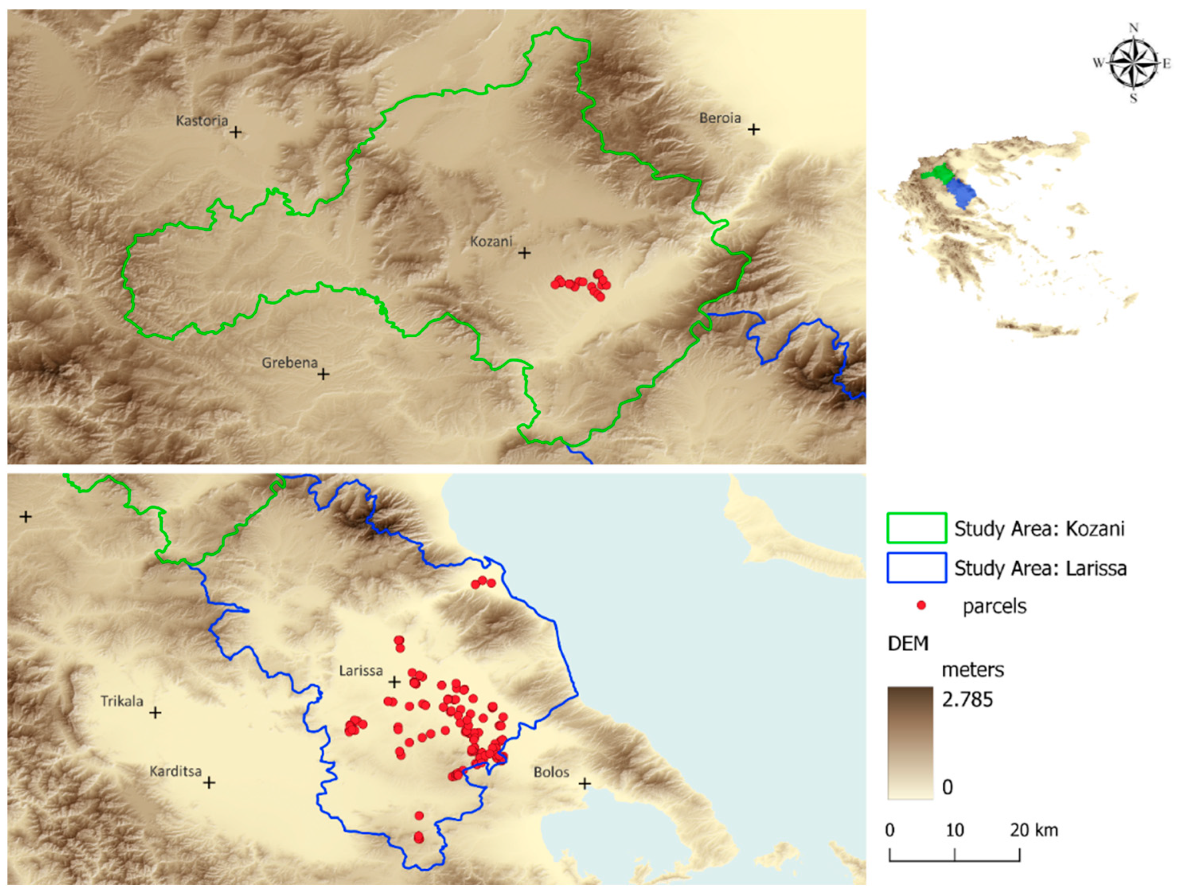
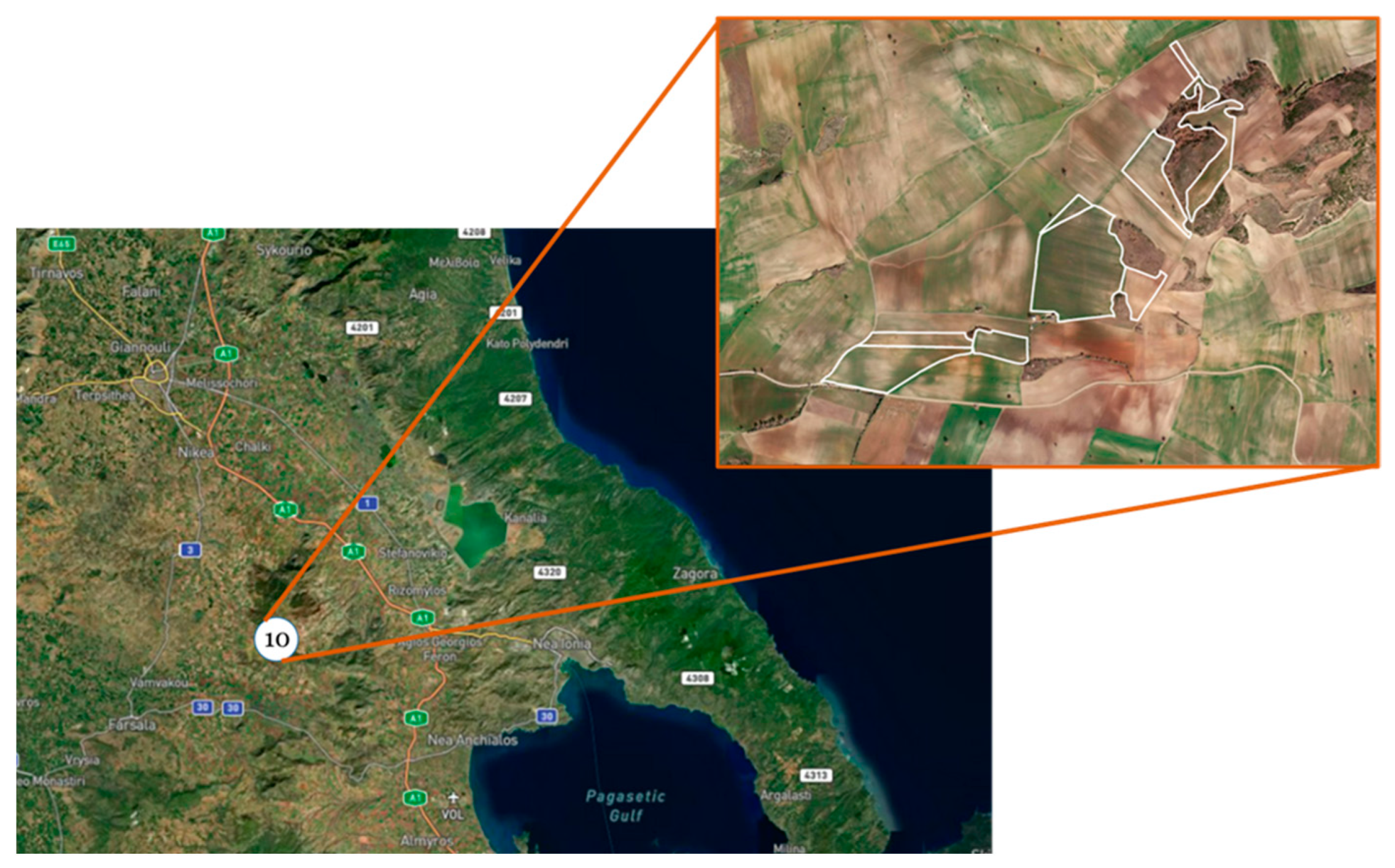
2.1. Study Sites and Parcels’ Data

Data from a total of 184 durum wheat parcels (Triticum turgidum subsp. durum) were used to evaluate the three modeling approaches. The parcels were located in the prefectures of Kozani (n = 22), northern Greece, and Larisa (n = 162), central Greece. The crops were established during the 2019/20 (n = 70 Larisa) and 2020/21 (n = 114 Larisa and Kozani) growing seasons, under contractual farming (Figure 1). In these regions, wheat and barley are the main winter crops (sown from October to December and harvested from mid-June to early July) grown in rotation with summer crops (e.g., cotton, maize, and sunflowers) [38]. Winter wheat is cultivated under rainfed conditions, but when water is available for irrigation, it is applied during flowering. This study included irrigated parcels (one irrigation event: n = 45 parcels; two irrigation events: n = 12 parcels). The irrigations were applied in their vast majority during the 2020–2021 growing season and only in Larisa region.

The climate of the selected sites can be broken down into two sub-types: (i) a lowland Mediterranean climate with drier summers and colder winters, and (ii) a continental Mediterranean climate with some of the continental climate characteristics typical of Balkan regions further north. This climatic variability found in Greece can be attributed to the complex topography. The rainfall pattern typical of Mediterranean coastal areas is characterized by dry spells in summer and a rainy season from mid-autumn to mid-spring [39].

The size of the parcels ranged from 0.1 to 10.5 ha. The geospatial data such as the location and perimeter of the fields; the final amount of production, which ranged from 500 to 6740 kg ha⁻¹; the sowing dates (3 November 2019 to 9 December 2019 and 25 October 2020 to 8 October 2020); the harvest dates (8 June to 31 June); and the irrigation dates and events were provided by Melissa Kikizas, SA. Rainfall during the 2019/20 growing season amounted to 509 mm in Larisa, while in 2020/21 it amounted to 450 mm in Kozani and Larisa, with significant variations in rain distribution between the two years and the two areas, especially during the flowering period (April–May). The average maximum daily temperature during the 2020/21 growing season in Kozani was 14.5 °C (−7.1 to 33.5 °C) and 15.8 °C (–0.9 to 32.4 °C) in Larisa, while in 2019/20 in Larisa it was 17.4 °C (5.2 to 38.4 °C). Based on official data, the average observed durum wheat yield in the region of Kozani is 2300 kg ha⁻¹, while for Larisa it is 3500 kg ha⁻¹.

Crop management included conventional soil tillage followed by seedbed preparation mainly with disc harrow and cultivator. Parcels were fertilized with approximately 120–150 kg N ha⁻¹ applied in split doses (60% before sowing as ammonium phosphate and 40% at the end of tillering stage as ammonium nitrate). Plant diseases and weeds were controlled by applying recommended fungicides (mainly in Larisa) and herbicides, at the doses suggested by their manufacturers.

2.2. Agro-Meteorological and Soil Data

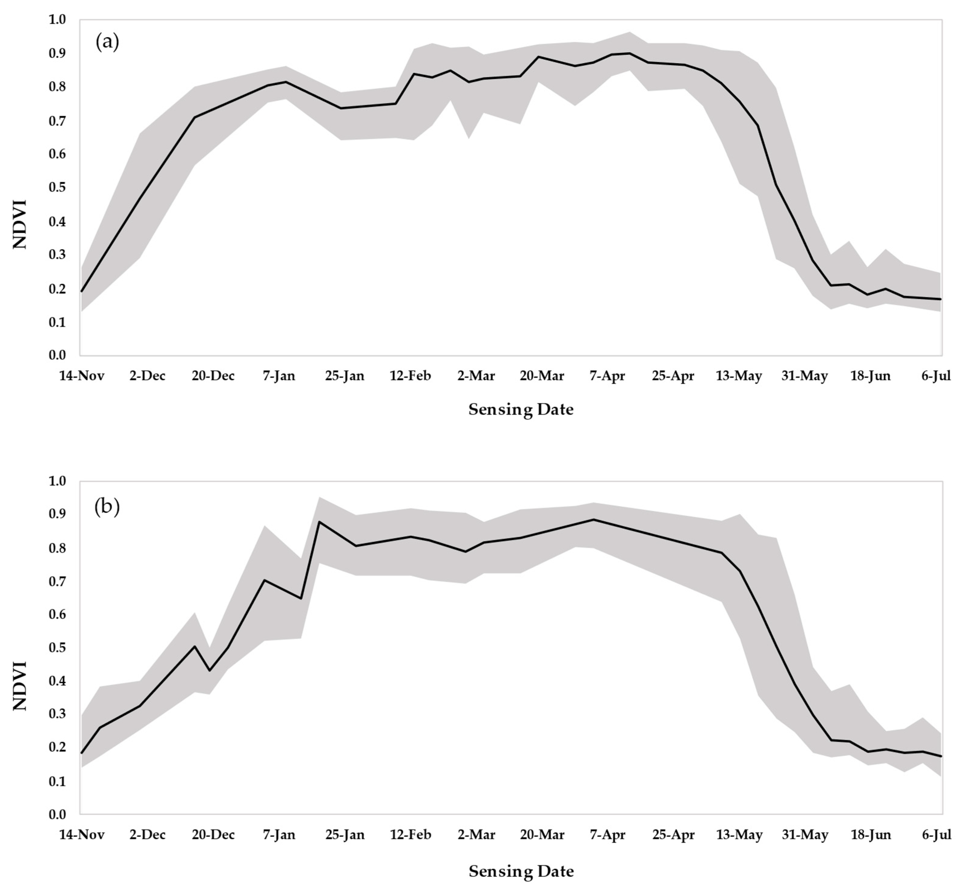
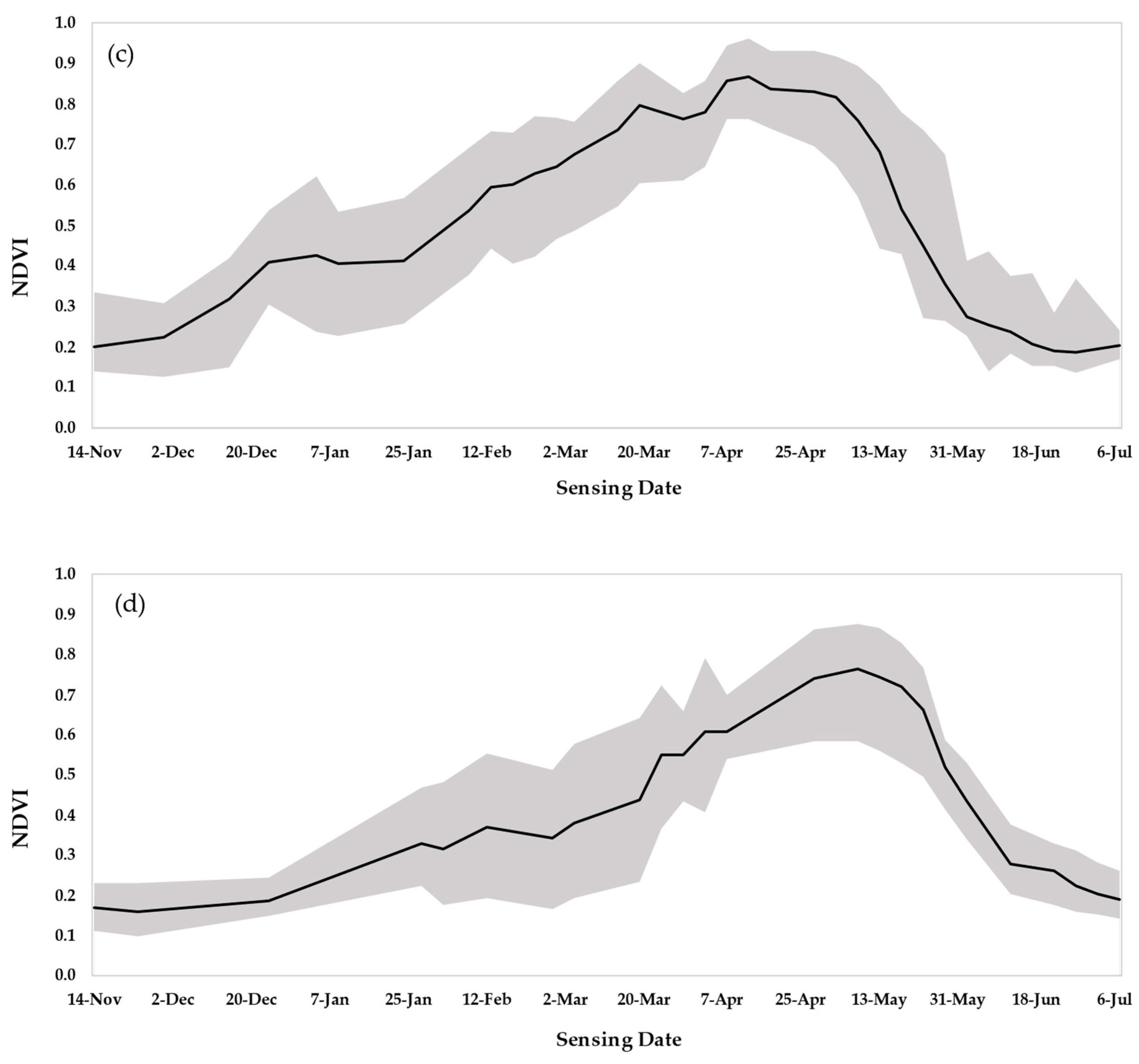
Gridded agro-meteorological data for the 2019/20 and 2020/21 growing seasons at a deg resolution of 0.1 × 0.1 (approx. 12.5 km) and of 0.25 × 0.25 (approx. 25 km) were derived from the ERA5-Land and ERA5 re-analysis, respectively, generated by the European Centre for Medium-Range Weather Forecasts and freely distributed through the Copernicus Climate Data Store. They included hourly data consisting of 2 m air temperature, total precipitation (at surface level), and all the necessary variables to obtain the reference evapotranspiration (ET_o) values with the Penman–Monteith equation proposed by the FAO56-PM. These parameters were aggregated into daily means and/or sums using Climate Data Operator (CDO) software [40]. Additionally, minimum and maximum daily air temperatures were derived. The growing degree days (GDD) of wheat were calculated by simple arithmetic accumulation of daily mean temperature above the base temperature value of 0 °C considered for wheat crop. GDD (°C) were calculated as suggested by [41]:

$$GDD=\frac{T_{max}+T_{min}}{2}-T_b$$

(1)

where $T_{max}$ and $T_{min}$ are the daily maximum and minimum temperature (°C), and T_b is the base temperature.

The soils’ physical properties for the 184 durum wheat fields were obtained from the SoilGrids database. SoilGrids is considered a convenient solution to obtain soil data because it is a gridded multiple depth dataset at a 250 m spatial resolution and it is available worldwide [42]. Soil information obtained from SoilGrids has been used in prior studies as a proxy for the determination of soil hydraulic properties [36,43,44]. The SoilGrids REST (representational state transfer) application-programming interface was used to request the products sand, silt, clay, bulk density, and organic carbon content at five standard layers (5–15, 15–30, 30–60, 60–100, and 100–200 cm). These soil properties were used to calculate soil water constants (field capacity, θ_FC, permanent wilting point, θ_PWP, and saturated hydraulic conductivity, K_sat) with the application of pedotransfer functions [45], representative of the soil profile layers (0–15, 15–30, 30–60, 60–100, and 100–200 cm).

2.3. Satellite Data

An average number of 25 and 22 cloud-free multispectral high-resolution images from Sentinel-2A and 2B were acquired during 2019/20 and 2020/21 wheat-growing seasons, respectively. The multi spectral instrument (MSI) on board the Sentinel-2A/2B captures data at 10, 20, and 60 m of spatial resolution over 13 spectral bands with a high temporal resolution of five days at the equator. Individual Sentinel-2, Level 2A granules were acquired from Copernicus Open Access Hub (https://scihub.copernicus.eu/), already ortho-rectified in UTM/WGS84 (image tiles of 100 × 100 km²). In order to obtain homogeneous and comparable products as time series, the vegetation indices NDVI (Normalized Difference Vegetation Index) and GreenWDRVI (Wide Dynamic Range Vegetation Index) were calculated based on atmospherically corrected Level-2A-Bottom-of-Atmosphere reflectance data. The images were cropped to the polygons’ (parcels’) geometry. NDVI and GreenWDRVI averages were assessed for pixels falling within each parcel, after excluding pixels affected by boundary effects. The equations to obtain the NDVI and the GreenWDRVI are as follows [46,47]:

$$NDVI=\frac{NIR-Red}{NIR+Red}$$

(2)

$$GreenWDRVI=\frac{a·NIR-Green}{\alpha ·NIR+Green}+\frac{1-\alpha }{1+a}$$

(3)

where $Red$ is the B4 band of Sentinel-2 MSI, Green is the B3 band, $NIR$ is the near-infrared B8 band of Sentinel-2 MSI, and a is a chlorophyll absorption coefficient, equal to 0.1. A 2nd-order polynomial relating the GreenWDRVI and $LAI$ (Leaf Area Index) [48] of wheat was used prior to determining the canopy cover:

$$LAI=5.7\cdot GreenWDRV{I}^2+1.7\cdot GreenWDRVI-0.08$$

(4)

Lastly, the canopy cover of wheat was estimated throughout the growing season with the exponential equation [49]:

$$C{C}_{RS}(\%)=94\cdot {\left[1-\exp \left(-0.43·LAI\right)\right]}^{0.52}$$

(5)

where $C{C}_{RS}$ is the canopy cover derived from spectral data.

According to the NDVI and reflected phenology, the wheat parcels were classified under 4 different growth dynamics patterns: 1. presenting a high initial growth rate; 2. a moderate initial growth rate; 3. a low initial growth rate; and 4. a very low initial growth rate observed in the Kozani region. A range of the average per parcel NDVI time series from the middle of November until the beginning of July is displayed in Figure 2a–d.

NDVI values assumed an upward trend from early December to the middle of April showing a high variability as the crop cycle progressed, with the highest being observed during the early reproductive stages. NDVI peak values and major ground cover were reached at different dates, even within the same year and region. Afterwards, a gradual decrease followed until early June and towards the harvest. It was noted that in almost all parcels a similar phenology was observed during the reproductive and maturity stages. A preliminary data analysis revealed that the wheat variety had little effect on the initial canopy development; thus, the growth rates were mainly affected by factors such as climatic conditions, soil properties, and to a lesser extent anthropogenic activities (e.g., sowing dates). The significant difference that is shown in the very low initial growth rate class [Figure 2d] is explained by the prevailing weather conditions in the Kozani region. Kozani has been built between the mountain ranges of Vermio, Burino, and Pieria, at an altitude of 720 m above sea level, whereas Larisa has an average altitude of 70 m above sea level and a typical Mediterranean climate with higher temperatures over the first months of the season, which allow for faster crop development during the initial wheat stages.

2.4. Yield Prediction with a Semi-Empirical Regression Model Based on Sentinel-2-Derived NDVI

Biomass is traditionally estimated through destructive, time-consuming, in situ methods; more recent estimates are based on remotely sensed data, such as vegetation indices (Vis). Many previous studies have examined approaches for within-season and post-season biomass and/or yield estimation using Vis [10,18,28,50,51]. In this study, relationships between Sentinel-2-derived NDVI and above-ground biomass were explored in order to determine the transfer function with the best fit for wheat yield estimation and to examine whether its results could be reproduced for different years and locations. To this aim, biomass data were collected for calibration and validation. The sampling campaign was conducted during the 2019/20 growing season. In situ above-ground biomass was collected from 10 parcels in the region of Larisa (Figure 3).

Measurements were conducted at weekly intervals during the wheat-growing season (October–May). At each parcel, 5 representative plants were collected from 3 randomly selected sampling sites; the plants were separated into leaves, stems, and grains and were dried in an oven for 48 h at 65 °C. The total dry biomass weight was averaged and multiplied by the number of plants per m² to calculate the biomass per square meter at each sampling point.

Cloud/shadow free Sentinel-2 images from sowing until harvest date were selected. For each measurement date, values of NDVI were extracted from the beginning of the growing season until the day plant biomass was measured. Sentinel-2 images within ±3 days of the ground data collection dates were considered acceptable.

The transfer functions were based on the cumulative VI approach, and in accordance with [20], the NDVI index was selected. NDVI is closely related to the vegetation vigor and has been recognized for its ability to monitor crops and as an estimator of crop yields since early 1980s. NDVI has an asymptotic non-linear relationship with the green LAI of some crops. A variation in LAI implies different intercepted radiation that, according to the radiation use efficiency, is directly related to the production of biomass that will determine the possible yield [52].

For each sampling parcel, the area under the curve, formed by the day of the year (DOY) and NDVI curve, was calculated through numerical integration, representing the value of the cumulative NDVI [20,53]. Several power transfer functions between cumulative NDVI and biomass were produced as regression functions. The derived models were evaluated using goodness-of-fit criteria, namely, coefficient of determination (R²), the root mean square error (RMSE), and the normalized RMSE (nRMSE) (see Section 2.6.1. Equations (8)–(10)). These measures indicate the degree of association between predicted and estimated values of the same parameter and give an indication of prediction efficiency [54,55]. In addition, Richter at al. [56] recommended this combined set of measures (R², RMSE, and nRMSE), amongst others, for the comprehensive quantification of vegetation biophysical models’ performance. The cumulative NDVI showed a moderate performance for the estimation of total dry above-ground biomass of durum wheat (RMSE: 389.4 kg ha⁻¹, nRMSE: 24.6%, R²: 0.68), yielding a power regression equation of the form:

$$Biomass \left({\mathrm{gm}}^{-2}\right)=3.1375·{\left[{{\displaystyle \int }}_{d_1}^{d_2}NDV{I}_{t}dt\right]}^{1.2874}$$

(6)

where $NDV{I}_t$ represents the NDVI curve, d₁ is the first day of the integral that coincides with the sowing date, and d₂ is the harvest date. Yield was calculated by the equation:

$$Yield \left({\mathrm{gm}}^{-2}\right)=0.42·Biomass$$

(7)

where 0.42 is the harvest index of durum wheat, selected as a representative of the dynamics of modern wheat varieties grown under Mediterranean conditions, such as the ones used in this study [57,58]. Previous studies have also reported similar results by fitting power or exponential regression equations to pairs of spectral indices and measured biomass [18,20].

The estimation accuracy of this transfer function, and its potential to be applied in different areas (regions of Larisa and Kozani) and different years (2019/20, 2020/21) was examined against yield data from the 184 wheat parcels.

2.5. Yield Prediction with a Machine Learning Data Fusion Model

Meteorological phenomena have the potential to significantly influence crop growth and yield [59]. In rainfed production systems such as those that include winter wheat, climate variability is responsible for as much as 80% of the variability in the agricultural production [60]. Consequently, understanding how the growth and development of rainfed wheat respond to climate variability, and employing various meteorological variables for early gross estimates of final yield, is of great importance for agricultural policy and market planning [22,61]. Simultaneously, biotic, genotypic, and management factors influencing crop growth reflected in crop phenology and development can be detected from satellite images. Therefore, the inclusion of remote-sensing observations can improve yield prediction by providing an opportunity for the real-time monitoring of crop growth status. ML algorithms have been widely used in crop yield prediction. ML regression models that use meteorological parameters (e.g., precipitation and temperature), remote sensing, soil conditions, and agricultural practices as explanatory variables have shown adequate ability to predict wheat yields [22,23,62,63].

In this study, weather data were combined with remotely sensed VIs for predicting field-scale wheat yields, adopting a number of ML regression algorithms, along with two time aggregation intervals (disaggregated or aggregated data) and two feature selection methods (based on Pearson Correlation Coefficient or SHAP feature importance). The regression algorithms used the following dependent variables: daily meteorological data ($T_{min}$, $T_{max}$, T_avg, ET_o, and Precipitation), the average NDVI (NDVI_avg) of the parcel, and whether or not irrigation was applied. Only parcels and yield data for the 2019/20 and 2020/21 growing seasons in the Larisa region (n = 162) were included in the inputs. The independent variable was the yield of the parcels in kg ha⁻¹. NDVI_avg values were linearly interpolated to generate a daily time-step NDVI time series. Then, the growing season was divided into crop growth stages based on the cumulative GDD (0–700 Pre-Tillering, 700–1000 Tillering, 1000–1450 Stem Elongation, 1450–1700 Booting, and 1700–2300 Flowering). Data from sowing to the end of flowering were used, aiming to predict the yield approximately one month before harvest. Then, two methods of aggregating the data were tested. The first received the average value of the input data throughout the selected growing period, while the second received the average value of the data for each crop growth stage separately. It was decided to follow the second method, as it showed slightly better interpretability.

Machine learning algorithms were fitted to the data using Scikit-learn, an open-source ML library. Nine estimators were evaluated, including: LR (Linear Regression), Ridge Regression (RR), Lasso (Least absolute shrinkage and selection operator), SVR (Support Vector Regression), KNN (K-Nearest Neighbors Regression), Decision Tree (DT), Random Forest Regression (RF), Gradient-Boosting Decision Tree Regression (GBDT), and eXtreme Gradient-Boosting Regression (XGBoost). LR is regarded as the benchmark statistical model. RR and Lasso apply L2 (squared magnitude of coefficients) or L1 (absolute value of the magnitude of coefficients) penalty terms to minimize overfitting and shrink the less important coefficients, respectively. SVR can minimize the error by making a hyperplane and maximizing the margin between predicted and observed values. KNN is a type of instance-based method that locates the k-closest points known to the model around an input sample to make the prediction. DT is an upside-down tree-like structure model that makes binary decisions to partition the data from the root node to the leaf nodes. RF is a bagging-based ensemble-learning technique combining a large set of decision trees that are built by selecting random features from the training dataset. GBDT and XGBoost are two implementations of ensemble methods based on gradient-boosting trees that make predictions sequentially and try to combine the weak predictive tree models.

2.6. Yield Prediction with a Process-Based Crop Growth Model: AquaCrop

AquaCrop simulates crop yield in four steps: crop development, crop transpiration, biomass production, and yield formation. It calculates the daily soil water balance and divides evapotranspiration into soil evaporation and crop transpiration. AquaCrop describes the foliage development of the crop by the canopy cover (CC_AC), which is the fraction of soil surface covered by the green canopy. Transpiration is a function of canopy cover, while evaporation is proportional to the area of soil not covered by vegetation. The canopy cover is multiplied by the reference evapotranspiration (ET_o) and the crop coefficient (K_c) to calculate potential crop transpiration. Actual transpiration (T_a) is calculated starting from the potential by accounting for water stress. Then, T_a is used for the calculation of crop biomass through its multiplication with water productivity normalized for climate. By using a harvest index, crop yield is obtained by the biomass [19,24,64,65]. A further detailed conceptual description of AquaCrop is available in Raes et al. [66], Raes et al. [66], and Steduto et al. [24]. Model parameters are grouped into two classes: conservative and non-conservative. Cultivar-specific or less conservative parameters vary depending on crop and field management, soil type, and climate (sowing date and density, length of crop cycle and phenological stages, maximum canopy cover, etc.). Conservative crop parameters do not change materially with time, management practices, and geographic location. The canopy growth (CGC) and canopy decline (CDC) coefficients are considered two of the most important conservative parameters to calibrate the CC_AC [67].

In this study, a number of non-conservative parameters were calibrated with regard to local management information, such as sowing dates and plant densities, flowering date and duration, and the onset of senescence and maturity. These parameters are provided in

Table 1. User-specific parameters used in simulation.

Parameter	Units	Default	Minimum, Medium, and Full Data Input
Soil surface covered by an individual seedling at (90%) recover	cm2/plant	1.50	1.50
Number of plants per hectare	Hm−2	4,500,000	2,500,000
Maximum canopy cover (CCx)	%	96	90–93
Calendar Days: from sowing to emergence	d	13	13
Calendar Days: from sowing to maximum rooting depth	d	93	93
Calendar Days: from sowing to start senescence	d	158	178
Calendar Days: from sowing to maturity (length of crop cycle)	d	197	221
Calendar Days: from sowing to flowering	d	127	150
Length of the flowering stage (days)	d	15	20
Maximum effective rooting depth	m	1.5	0.3
Reference Harvest Index (HIo)	%	48	42
Water productivity (WP)	gm-2	15	17

. The model was applied under Calendar Days (CD) mode. Water stress was the only growth-limiting factor considered during AquaCrop implementation. Soil data were retrieved from the SoilGrids database, up to a soil profile depth of 2 m, for each parcel.

Three runs were performed per parcel containing different levels of information:

• CGC and CDC retrieved from AquaCrop default values on wheat without considering any irrigation event (minimum data input);
• CGC and CDC calibrated to the canopy cover derived from remote-sensing data (CC_RS) without considering any irrigation event (medium data input);
• CGC and CDC calibrated to CC_RS, including the irrigation events (one event: n = 45 parcels; two events: n = 12 parcels) applied during the 2020/21 growing season (full data input).

The purpose of the selected simulations was to investigate the potential of AquaCrop to predict biomass and yield under a minimum, medium, and full input data scheme.

Canopy cover data can be derived from empirical relations with different VIs based on satellite measurements in the optical and near-infrared bands. In particular, the 30 m Landsat data [68], the 10 m Sentinel-2 data [69], and the 3 m PlanetScope data [70,71] have been extensively used in agricultural applications [72]. Many studies assimilated directly [19,73] or adjusted [67,74] canopy cover in AquaCrop, either from field measurements or remote-sensing data. In this study, representative CC_RS curves of the different wheat growth classes were selected to calibrate the CGC and CDC, thereby enabling a full exploitation of satellite data. During calibration, these parameters were varied until satisfactory agreement was achieved between CC_RS and simulated CC_AC, verified by the statistical metrics panel of AquaCrop (Figure 4). The calibrated values are provided in

Table 2. Calibrated conservative parameters of AquaCrop used in simulation.

Conservative Parameters	Units	Default	Medium and Full Data Input Scheme
Canopy growth coefficient (CGC)	Fractiond−1	0.049	High Initial Growth class	0.085
			Moderate Initial Growth class	0.069
			Low Initial Growth class	0.054
			Very low Initial Growth class	0.035
Canopy decline coefficient (CDC)	Fractiond−1	0.0718	High Initial Growth class	0.0605
			Moderate Initial Growth class
			Low Initial Growth class
			Very low Initial Growth class

. The same value was kept for the CDC in all classes, since the reduction in NDVI in the wheat parcels follows approximately the same trend during senescence.

2.6.1. Performance Evaluation Metrics

The ability of AquaCrop to predict yield was assessed by adopting a number of statistical metrics. The Model Efficiency (ME) [75], the coefficient of determination (R²), the root-mean-square error (RMSE), the normalized RMSE (nRMSE), the bias, and the Willmott’s index of agreement (d) [76] were selected as performance evaluation metrics. These metrics are mathematically expressed as:

$$ME=1-\frac{{\sum }_{i=1}^n{\left(x_i-y_i\right)}^2}{{\sum }_{i=1}^n{\left(x_i-x_{avg}\right)}^2}$$

(8)

$$R^2=\frac{{\left({\sum }_{i=1}^n{y}_i-y_{avg}\right)}^2}{{\left({\sum }_{i=1}^n{x}_i-y_{avg}\right)}^2}$$

(9)

$$RMSE=\sqrt{\frac{{\left({\sum }_{i=1}^n{x}_i-y_{avg}\right)}^2}{n}}$$

(10)

$$nRMSE=\raisebox{1ex}{$\sqrt{\frac{{\left({\sum }_{i=1}^n{x}_i-y_{avg}\right)}^2}{n}}$}\!\left/ \!\raisebox{-1ex}{$y_{avg}$}\right.$$

(11)

$$ias=\frac{1}{n}{\displaystyle \sum }_{i=1}^n\left(y_i-x_i\right)$$

(12)

$$d=1-\frac{{\sum }_{i=1}^n{\left(y_i-x_i\right)}^2 }{{\sum }_{i=1}^n{\left(\left|y_i-x_{avg}\right|+\left|x_i-x_{avg}\right|\right)}^2}$$

(13)

where $x_i$ is the $i$_th measurement, $y_i$ is the corresponding model estimate, $y_{avg}$ is the mean value of the model estimates, $x_{avg}$ is the mean value of the measurements, and n is the number of samples. Generally, the larger R² is, the better the model’s fit is. The ME is a measure of the mean square to the observed variance. The smaller the departure from ($x_i$–$x_{avg}$), the higher the performance efficiency of the model. Values of ME range between 1 and –∞, where ME = 1 denotes perfect model fit and ME = 0 means that the error is the same magnitude as the observed variance and the observed mean value is as good a predictor as the model. The ME has no lower limit. The RMSE and the bias have the same unit as that of the variable being simulated. The closer the RMSE is to zero, the better the model’s simulation performance. The range of the nRMSE metric generally defines the model’s accuracy. A value of nRMSE  <  10% indicates that the estimated and measured values are highly consistent, the range 10%  <  nRMSE  <  20% indicates good consistency, while the range 20%  ≤  nRMSE  < 30% indicates medium consistency, and finally nRMSE  ≥  30% indicates poor consistency. The bias refers to the tendency of overestimation or underestimation and d represents the ratio of the mean square error and the potential error (1 indicates a perfect match, and 0 indicates no agreement).

3. Results

3.1. Evaluation of the Semi-Empirical Regression Model

The wheat yield datasets from the 2019/20 and 2020/21 growing seasons were selected to validate the estimation accuracy of the derived transfer function. The statistical analysis, presented in

Table 3. Statistical evaluation of the transfer function (n = 184).

Statistical Metric	Units	Results
Average estimates	kg ha−1	3720
Average measured	kg ha−1	3774
std estimates	kg ha−1	811
std measured	kg ha−1	1252
Value range estimates	kg ha−1	1450–5320
Value range measured	kg ha−1	500–6740
RMSE	kg ha−1	1076
nRMSE	%	28.5
R2	–	0.26

, revealed moderately strong correlations (RMSE, nRMSE, and R² equal to 1076 kg ha⁻¹, 28.5%, and 0.26, respectively) between the estimated and measured wheat yields. The RMSE range of 697 to 444 kg ha⁻¹ and nRMSE values as high as 27% have been reported [28] for rainfed wheat and barley yield estimations with the cumulative NDVI approach applied to Spain. Linear models relating the MODIS NDVI and wheat yield, calibrated with different growing season data in Argentina, resulted in a wide range of R² values from 0.08 to 0.69 when applied for inter-annual yield estimation [29]. The researchers supported that the inter-annual variation observed indicates the influence of agrometeorological conditions on the yield estimation by the NDVI. A previous study [77] used NDVI and weather data to estimate the wheat yield in Morocco and found that the NDVI appeared to contain most of the information on rainfall and explained most of the grain yield variability.

In this study, environmental and management—rather than genotype—factors were considered significant for explaining the variability in the final received yield, both within the same region and between regions (Larisa and Kozani). The predictability of the grain yield by the transfer function was affected by these factors, which reflect differences in yield formation, as a main response to the limited water availability during flowering and grain filling (2020/21 growing season). However, these differences could not be reflected in the wheat canopies with high and moderate initial growth rates (n = 121). This is also evident in the statistical results received after the exclusion of irrigated parcels. In this case, the calculated metrics only slightly improved (RMSE, nRMSE, and R² equal to 983 kg ha⁻¹, 28.6%, and 0.37, respectively). This indicates that any management decision received slightly before or during flowering to improve the final yield (irrigation and/or growth regulators) did not result in an equal adjustment of the phenology curve because the NDVI had already reached high values by that time. The NDVI increased until the onset of flowering, receiving the highest values by early to mid-April, while also determining most of the cumulative NDVI, which is calculated by the area under the curve.

Studies support that at the grain-filling stage, the NDVI decreases up to 0.3 because the crop becomes stressed and its capacity to absorb PAR is reduced [78]. Since the area under the curve becomes considerably steep after the reproductive stage, the contribution of the cumulative NDVI in Equation (6) becomes minimal during this time period, hardly affecting the final estimated yield. Therefore, this method is able to predict the final yield’s magnitude approximately 40 days before harvest. The calculations continue throughout the growing season and the prediction improves as new cloud-free satellite images become available until harvest. The results demonstrate a clear potential to operationally predict the levels of the final yield when reaching the end of the growing season. Though the prediction accuracy can be characterized as low with 20% < nRMSE < 30%, the estimated biomass can be interpreted to yield, which can then be visualized per pixel in productivity maps immediately after sowing. The real-time acquisition and spatial continuity of remote-sensing data can effectively enhance the applicability of such regression relationships between biomass and spectral indices at regional scales. Furthermore, the estimated biomass can be used to optimize the crop parameters used in crop growth models to obtain the optimal simulated biomass.

3.2. Evaluation of the Machine Learning Estimator

Due to the small sample size (n = 162 parcels), as well as the structure of the data, it was decided to evaluate the models using the Leave-One-Out Cross Validation (LOO CV) method, as the separation into training/testing validation would lead to biased subsets. Both data aggregation methods were tested in terms of accuracy: 1. using the mean parameter values from sowing until approximately one month prior to harvest as inputs and 2. using the mean values of the pre-determined crop growth stages as inputs. The coefficient of determination, R²_train, and RMSE_train (Equations (9) and (10)) between the predicted yield and the observed yield were used for the models’ performance evaluation. Firstly, the LOO CV based on the training data was evaluated, because this procedure can estimate the robustness and generalization of the models. Secondly, the same evaluation method based on the test data was implemented (R²_test and RMSE_test). After fitting the ML estimators to the input data, the statistical criteria were calculated and the ones with the best performance are provided in

Table 4. Statistical evaluation of yield estimates with the best-performing ML algorithms for parcels in the region of Larisa (n = 162).

Data Aggregation	Algorithm	RMSEtest (kg ha−1)	Std(RMSE) (kg ha−1)	R2test	RMSEtrain (kg ha−1)	R2train
Mean parameter values from sowing until one month prior to harvest	Random Forest (RF)	558.6	393.1	0.64	207.2	0.95
Mean parameter values using as input the mean values of each crop growth stage	eXtreme Gradient Boosting (XGBoost)	526	376.3	0.68	0.001	1

.

An attempt was made to select features both by the criterion of the importance that the respective model assigns to the features (feature importance) and with the SHAP values. Although features that did not make a significant contribution to performance prediction and are theoretically a source of noise were removed, both the interpretability and prediction accuracy decreased.

From the statistical evaluation of the above findings regarding the performance of the ML algorithms with respect to the estimation of yield, the phenomenon of overfitting is evident. That is, while the model trains well on existing data, it fails to reliably predict new data that is unknown to it. This phenomenon is due both to the small size of the dataset compared to the complexity of the problem and to its structure. The results from this approach suggest that the ensemble learning methods RF and XGBoost achieve the best performance and this finding is in agreement with previous studies. Ruan et al. [63] included eleven statistical and machine learning techniques for predicting field-scale wheat yield and found that the two ensemble learning models RF and XGBoost were most accurate in prediction, with R² values in the range of 0.74–0.78 and RMSE values in the range of 780–850 kg ha⁻¹. Cao et al. [79] adopted MLR, XGBoost, RF, and SVR algorithms and three datasets including MODIS EVI, climate data, and the subseasonal-to-seasonal (S2S) atmospheric prediction data to estimate winter wheat yield. The results showed that among the four models, XGBoost possessed the highest skill with the S2S prediction as inputs, with an R² of 0.85 and an RMSE of 780 kg ha⁻¹. Ang et al. [80] employed the RF and AdaBoost algorithms to estimate oil palm yield prediction from multi-temporal remote-sensing data. The results of the study revealed that the RF model outperformed the AdaBoost model. Kamir et al. [81] used nine base learners and two ensemble (average ensemble and Bayesian fusion) methods to estimate wheat yields across the Australian wheat belt from climate data and satellite image time series. The results showed that SVR with a radial basis function emerged as the single best learner with an R² of 0.77 and RMSE of 550 kg ha⁻¹ at the pixel level, and the ensemble techniques did not show a significant advantage over the single best model.

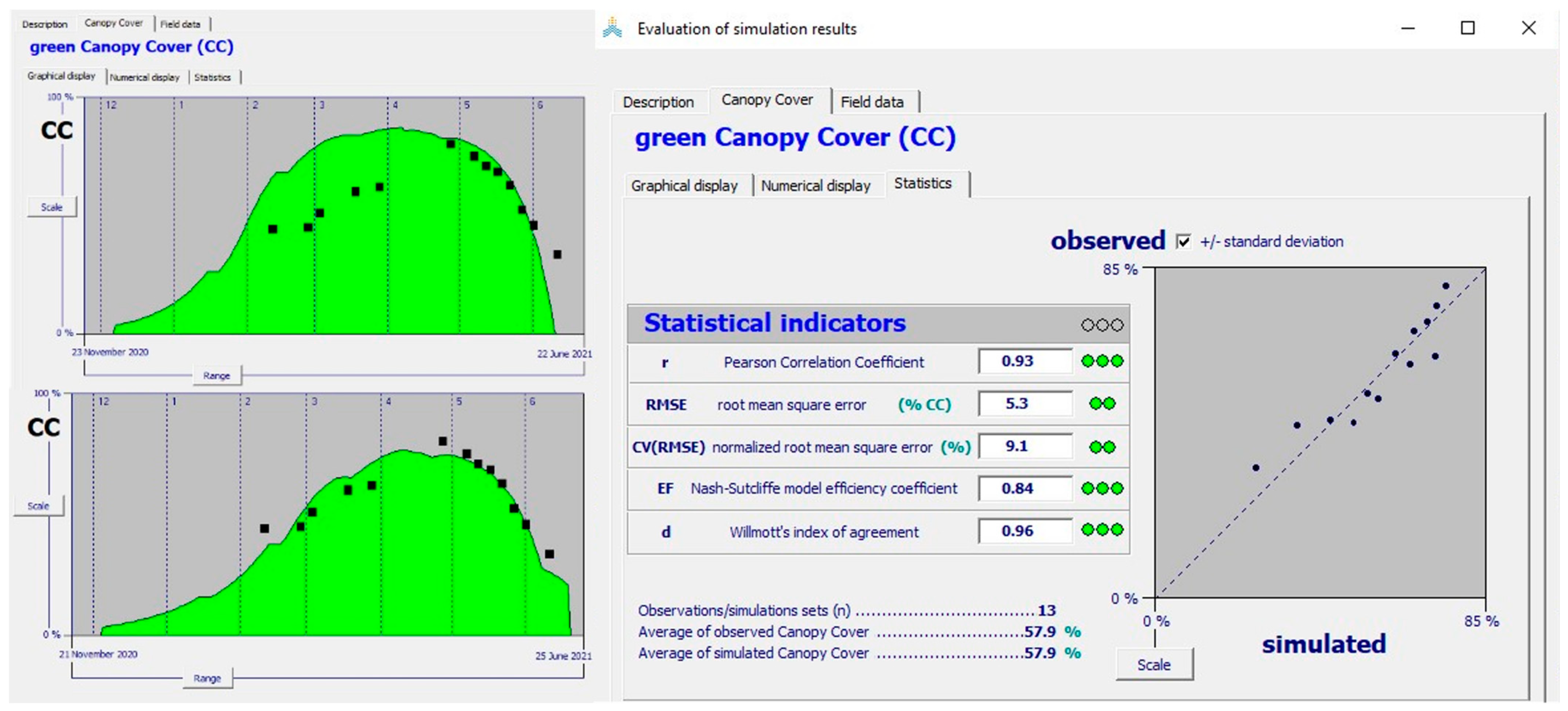
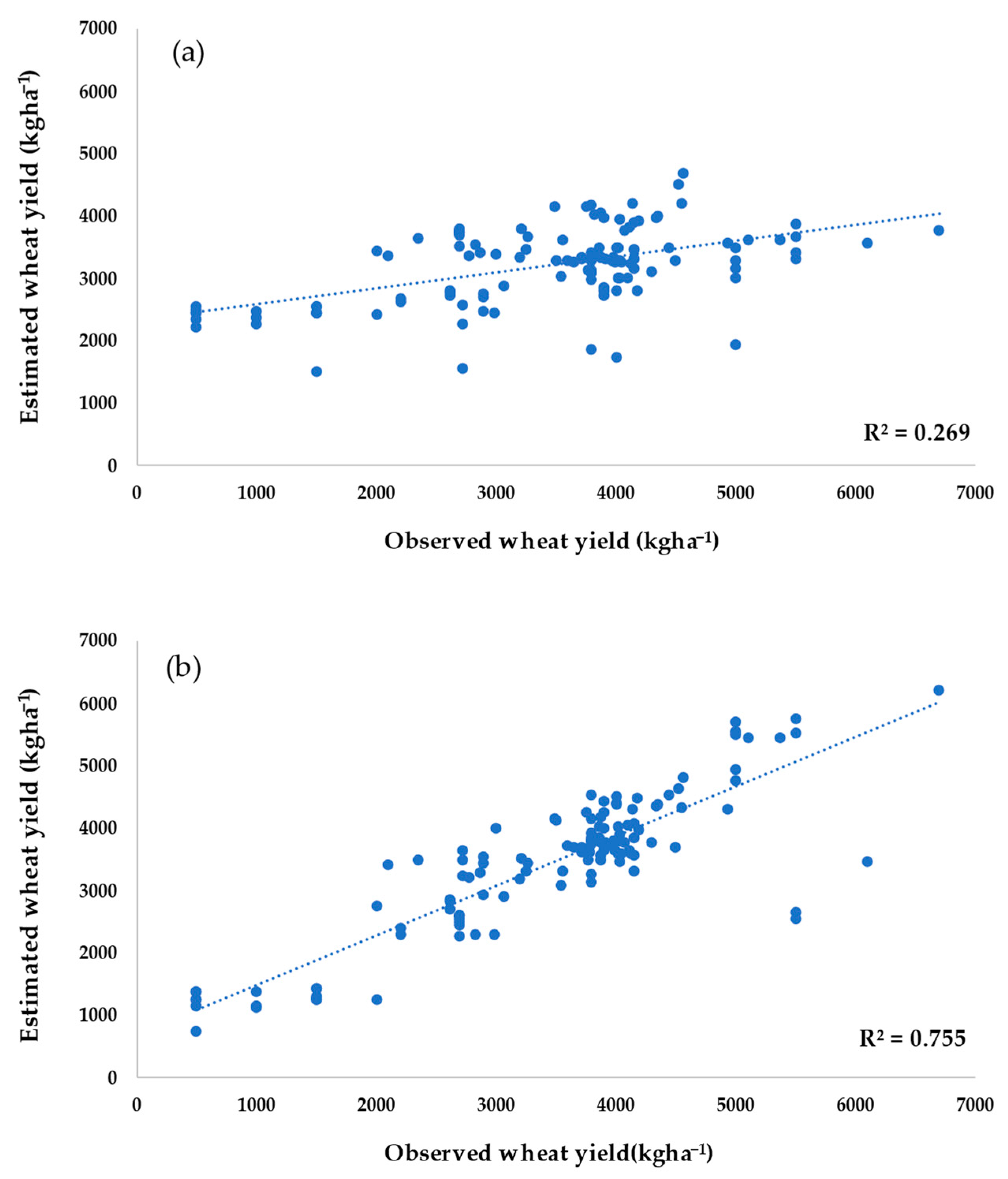
3.3. Evaluation of AquaCrop for Yield Prediction

AquaCrop was evaluated for yield prediction under a minimum, medium, and full data input scheme. The calculated statistical metrics that were employed to evaluate the goodness of fit in these approaches are summarized in

Table 5. Statistical evaluation of yield estimates with AquaCrop (n = 184).

Statistical Metric	Units	Minimum Data Requirements	Medium Data Requirements	Full Data Requirements
Average estimates	kg ha−1	3080	3110	3731
Average measured	kg ha−1	3774	3774	3774
std estimates	kg ha−1	757	1067	1150
std measured	kg ha−1	1252	1252	1252
Value range estimates	kg ha−1	850–4670	750–4810	750–6370
Value range measured	kg ha−1	500–6740	500–6740	500–6740
ME	−	−0.4	0.4	0.8
RMSE	kg ha−1	1500	996	569
nRMSE	%	39.6	26.5	15.1
bias	kg ha−1	−70.6	−38.6	−4.31
d	−	0.485	0.827	0.942
R2	−	0.05	0.50	0.80

. The reason to follow a minimum data requirements framework was to investigate whether the model has the potential to provide safe results through a simplified approach with respect to data intensiveness. Winter wheat is a typical rainfed crop for Greece and the Mediterranean region in general [82]; however, in order to achieve high yields, farmers apply water, usually originating from deep boreholes that are used for irrigation purposes. Data on the timing and amount of applied water is scarce, leading inevitably to yield simulation uncertainties in regional and large-scale applications. The aim of this approach was to reduce the calibration workload and facilitate simulation when the parcel-level management conditions are unknown—especially irrigation events, since zero fertility stress was assumed and crop phenology was provided as a common characteristic of the studied wheat varieties. Previous studies have also investigated the potential of AquaCrop to estimate biomass and yield under limited field-based data availability [72,83]. A successful minimum or at least medium input simulation could encourage the regional implementation of the model, which could drive in-season and post-season adaptation strategies for food security. However, in the case of a minimum data requirements scheme, the statistical metrics between the measured and simulated values (Table 5) revealed that AquaCrop could not simulate wheat yield successfully. This is indicated by the low values of the ME, bias, d, and R² of −0.4, −70.6, 0.485, and 0.05, respectively, as well as a high absolute and relative magnitude of difference between the simulated and measured final yields (RMSE = 1500 kg ha⁻¹ and nRMSE = 39.6%). The under-calibrated model significantly underestimated yield, which can be attributed to the limited rainfall and heat stress during the flowering and grain-filling stages in 2020/21 that resulted in the prediction of very low yields. The high yield levels obtained by irrigation (>4500 kg ha⁻¹) during 2020/21 could not be achieved by the model running under rainfed mode, leading to large prediction inaccuracies.

On the other hand, a medium data requirements scheme was applied, based on a calibrated simulation of canopy cover, because it is central to AquaCrop performance, as it affects the rate of transpiration and, consequently, biomass accumulation and final yield prediction. The calibration of CC_AC led to a significant improvement of the statistical metrics. Specifically, the tendency to underestimate was reduced from −70.6 to −38.6 and the R² increased from 0.05 to 0.50, thus indicating that the calibrated CC_AC model better explained the variance of the observed yield values. The estimation errors also decreased, with the nRMSE decreasing from 39.6% to 26.5%, the RMSE decreasing from 1500 kg ha⁻¹ to 996 kg ha⁻¹, and the ME increasing significantly from −0.4 to 0.4.

In spite of the improved accuracy obtained with the calibration of the CC_AC, the results still discourage the large-scale and limited data availability applications of the model. However, by excluding the irrigated parcels from the statistical analysis (

Table 6. Statistical evaluation of yield estimates with AquaCrop only for rainfed parcels (n = 127).

Statistical Metric	Units	Minimum Data Requirements	Medium Data Requirements
Average estimates	kg ha−1	320	343
Average measured	kg ha−1	345	345
std estimates	kg ha−1	600	1128
std measured	kg ha−1	1233	1233
Value range estimates	kg ha−1	1500–3200	750–6220
Value range measured	kg ha−1	1250–6700	1250–6700
ME	–	0.2	0.8
RMSE	kg ha−1	1086	616
nRMSE	%	31.5	17.9
bias	kg ha−1	−24.4	1.3
d	–	0.623	0.930
R2	–	0.27	0.75

), the results obtained with the CC_AC calibration improved significantly and became comparable with those reported in previous studies. The RMSE values of 616 kg ha⁻¹ and ME of 0.80 are consistent with the ranges reported by Xing et al. [84] (330 to 580 kg ha⁻¹), as well as the model efficiencies of 0.78 when the researchers applied AquaCrop for wheat yield simulation. RMSE values of 580 kg ha⁻¹ (nRMSE = 11.9%) were also calculated by Iqbal et al. [85] who applied AquaCrop for three years of wheat cultivation. A study conducted to assess the performance of AquaCrop to simulate the spring wheat yield in Western Canada [86] produced R² and RMSE values of 0.66 and 743 kg ha⁻¹, respectively. Lower RMSE values of 320 kg ha⁻¹ and ME of 0.82 were found for a grain yield simulation under varying water regimes on winter wheat in Turkey [87]. RMSE, nRMSE, and R² values of 550 kg ha⁻¹, 8.77%, and 0.82, respectively, were found by the assimilation of winter wheat biomass retrieved from remote-sensing data via AquaCrop, in Beijing, China [18]. AquaCrop was calibrated and evaluated for yield prediction in a field experiment of spring wheat for two growing seasons in Egypt, producing RMSE, d, and R² values of 555 kg ha⁻¹, 0.93, and 0.84, respectively [88].

Figure 5a,b show the linear correlation between simulated and observed grain yield for the 127 rainfed wheat parcels. In the calibrated CC_AC, the linear trendline deviates slightly from the desirable straight line, x = y, and thus has a high coefficient of determination, R², at 0.75.

Although there was a rather extensive simplification employed to make the model less data intensive, the metrics of Table 6 clearly indicate the need for a careful calibration of the CC_AC to reduce errors and bias when simulating grain yield. In fact, in this case, it is remarkable that the CC_AC calibration very successfully simulates a wide range of yields, from the very low (750 kg ha⁻¹) to high (6220 kg ha⁻¹) levels, obtained from rainfed parcels. The adjustment of the CGC, CDC, and CC_x shows a great potential for simulating yields of different wheat varieties with varying growth patterns under multiyear and multi-environmental conditions.

Finally, a full data input scheme was evaluated, which combined the calibrated CC_AC with actual irrigation data. Due to the precipitation scarcity during the 2020/21 growing season, irrigation was applied to wheat during spring to secure the wheat’s water demands. The irrigation events took place between April and early May, before and during flowering. The results show that a very good agreement was obtained by AquaCrop regarding the simulation of the grain yield for the 184 wheat parcels, excelling in performance all studied cases. This is attributed to the high potential of AquaCrop, as a water-driven model, to predict elevated yield levels with a detailed soil water regime. Several authors [74,89,90,91,92] have reported very good simulation results with AquaCrop applied for irrigated crops, compared to rainfed and water deficit treatments.

The results suggest that AquaCrop can be implemented as a convenient model for deciding whether wheat is rainfed or irrigated during dryer growing seasons, provided that the records of the timing and amount of irrigation are available from the farmers. If such records are unavailable, remote sensing can still be a solution for detecting irrigation events [93,94], thereby either partially or fully automating the process of crop growth simulation. AquaCrop offers a balance between accuracy obtained with mechanistic models and robustness, and can be a valuable tool for yield prediction, particularly since it requires a relatively small number of explicit data that can be readily available or easily interpreted to obtain valuable information [74,86].

4. Discussion

In this study, three modeling approaches were investigated and evaluated with respect to their potential for in-season or post-season in-field yield estimation, as well as their applicability at a large scale. Remotely sensed satellite data are often used to retrieve variations in vegetation states by providing realistic information on photosynthesis, phenology, disturbances, recovery, and human interventions [95,96]. The remotely sensed extraction of winter wheat growth patterns and phenology has a strong foundation in the three studied modeling approaches. Many previous works supported that the use of calibration techniques based on remote sensing improves yield assessments from crop growth models such as AquaCrop [91,97]. The most logical pathway for a systematic calibration of AquaCrop is first and foremost to ensure a sound prediction of canopy cover. The key user-input parameters for this purpose are the coefficients defining the canopy development, with particular attention to its shape. In this study, the canopy cover data were derived from empirical relations, with spectral vegetation indices acquired from satellite images covering 184 wheat parcels. The yield prediction via AquaCrop significantly improved when a proper calibration of the CC_AC curve parameters (CGC, CDC, and CC_x) was performed, based on the wheat growth rates reflected in the NDVI. Different hybrids/varieties of the same crop often show some similarities regarding the relative development and duration of growth stages, despite discrepancies in the length of the growing seasons. This implies that the parameter values calibrated for one crop hybrid/variety could potentially be useful for the simulation of another with some adjustment, which may reduce the burden of parameter calibration [83]. To this aim, this work provided pairs of values for the difficult-to-determine canopy parameters for the further testing and use of the model with a wide range of wheat varieties and growth habits in response to environmental, management, or genotypic factors, as well as biotic or edaphic stresses. The calibrated AquaCrop results, although obtained with a medium data input load, were comparable with those reported in the literature for more detailed field experiments and treatments. It is challenging for simulation models to find relevance in real world agriculture; however, the current work suggests that the combined simplicity and accuracy of AquaCrop [98] make the model an indispensable tool within decision support systems for a broad usage by end-users.

Large scale applications require intensive field work and in situ campaigns that are known to require a large number of personnel, a high degree of logistical support, machinery and equipment, and, thus, huge budgets, which increase with the increasing area of the study site. In this context, apart from the identified significant contribution of remote sensing, the findings of this study also prove that gridded datasets on soil, such as SoilGrids, as well as environmental conditions, such as ERA5-Land and ERA5 reanalysis, can operationally be employed for large scale applications through a wide range of modeling approaches. These datasets are the result of multiyear research, present improved accuracy and resolution of spatially explicit data, are updated regularly, and are freely available from different initiations and official online websites. The coupling of these datasets for the simulation of the durum wheat yield in 184 parcels presented high prediction accuracies, which are similar to those found in the literature using detailed weather station meteorological data or soils’ physical properties derived from laboratory-analyzed soil samples as inputs. SoilGrids and ERA5-Land or re-analysis data can support operational platforms for dynamic crop monitoring and yield forecasting operating at the administrative level by government agencies, non-governmental organizations, farmers’ unions, agri-food industries, and consultants [35,36]. With the advancement of computational ability, these operational systems can acquire real-time satellite data; collect soil and agro-meteorological products; perform preprocessing and analysis; run cloud-based machine learning algorithms or crop growth models (e.g., AquaCrop-OS) [99]; perform in-season, post-season, and even seasonal crop yield predictions; and generate the final outputs.

The other, less data-intensive approach studied in this work involves the development and application of a semi-empirical transfer function for a yield assessment. Though the prediction accuracy indicates medium consistency with the measured yield data, i.e., 20% < nRMSE < 30%, the method is a good tool for predicting the levels of the final yield before harvest, at a regional level. In addition to the timeliness and spatial scale, ideal yield predictions also depend on rapid methods and accessible data. This method can fully exploit Landsat and Sentinel-2 satellites that provide high spatial resolution imagery data (10–30 m) with relatively short revisiting periods. This suggests that the method acquires satellite data as they become available during the growing season and calculates biomass and yield to provide dynamic yield forecasts at a fine scale. The method used in this study allows researchers to predict wheat yield levels approximately 40 days before harvest at the seed-filling stage. A common desire is to have in-season or post-season predictions of anticipated yields over large geographic regions for various purposes, namely, (a) to support the timely management of food shortages and strategic actions planning; (b) for the identification of low productivity farms and parcels and, thus, as a basis for implementing optimization strategies for the following season; (c) to facilitate the planning of harvesting logistics, for example, to estimate the required number of transport vehicles, available silos, or storage locations and, thus, to reduce the costs associated with the transportation and storage of grain; (d) to optimize the price of the commodity according to its availability and the harvested amounts; and (e) to inform decisions on trade, potential industry growth, and investment [10]. In general, the NDVI transfer function perceived the temporal and spatial variability in the study area; however, it was unable to identify the management factors that promote yield because it relies on phenology and such actions are not followed by relative adjustments on the spectral reflectance curves. Furthermore, the difficulty in predicting low yield values as a result of environmental factors indicates the necessity of a possible coupling with agrometeorological data in order to obtain scalability and additional accuracy in yield estimations. This requires further research, especially in order to use the minimum number of inputs and available data.

ML methods are advantageous considering their high accuracy and wide applicability; however, they often serve as a “black-box” method, as the resulting rules for obtaining the results are often too complex or concealed to be readily interpreted. In addition, they rely heavily on training samples (particularly deep learning algorithms), and the sample sizes demanded are large. In this study, a number of machine learning methods were tested for yield estimation. However, the number of training samples was considered low, leading to overfitting of the data. This indicates that additional training data are required to further improve the skill of the models. Furthermore, the aggregation approach and feature selection methods did not significantly affect the yield prediction performance for the selected ML methods. As previous studies have illustrated [63,81], ML methods are promising frameworks that can complement regional scale models and provide valuable insights into understanding yield responses to environmental conditions; however, more reliable publicly available data are needed to further enhance the accuracy and implementation of large-scale yield prediction.

5. Conclusions

This study presents three methods of winter wheat yield estimation presenting different levels of input data intensity based on predictors originating from open-access satellite data, SoilGrids, ERA5-Land, and ERA5 climate reanalysis. These methods could potentially be fully automated crop yield-forecasting systems, operating at the administrative or regional unit scales. The methods were validated with 184 durum wheat yields in two distinct regions in Greece, namely, Larisa and Kozani. The analyzed period covered two growing seasons: 2019/20 and 2020/21; however, the availability of the data differed among the regions. The main insights from this study are as follows: (i) medium input data intensity models can provide high to moderate accuracies for yield estimation, thus minimizing the time, cost, and labor of data acquisition; (ii) free access datasets are excellent sources of input data for satisfying models’ requirements, especially ones running under cloud-computing environments (e.g., DIAS or Amazon AWS), where these datasets are directly accessible; (iii) remote sensing offers an unprecedented ability for the proper parameterization of the CC_AC curve parameters of the AquaCrop model, leading to significantly improved simulations of crop biomass and yield, under different environmental conditions; (iv) the AquaCrop model, as well as the spectral index transfer function, can be used with a high to acceptable degree of accuracy for the regional yield simulation of winter wheat, and can serve as useful tools for assessing food security in the agricultural sector; (v) although wheat is considered a rainfed crop, any irrigation event applied to promote yield cannot be reflected on the spectral behavior of the canopies (especially ones performed slightly before or during flowering) and, thus, records of time and the amount of water are required to achieve high yield estimation accuracies; and (vi) due to the complex structure of machine learning, it is still challenging to provide reliable estimates for final yield formation, since more training data are required to reach high accuracies. In summary, the results indicated that medium input data intensity methods are effective tools for operational, large scale yield assessments of winter wheat. Although wheat is one of the key crops grown worldwide, further studies are needed to verify these results for different crops and in different ecological areas.

References

1. Challinor, A.; Watson, J.; Lobell, D.; Howden, S.M.; Smith, D.R.; Chhetri, N. A meta-analysis of crop yield under climate change and adaptation. Nat. Clim. Chang. 2014, 4, 287–291. [Google Scholar] [CrossRef] [Green Version]
2. Berry, P.; Yassin, F.; Belcher, K.; Lindenschmidt, K.-E. An Economic Assessment of Local Farm Multi-Purpose Surface Water Retention Systems under Future Climate Uncertainty. Sustainability 2017, 9, 456. [Google Scholar] [CrossRef] [Green Version]
3. Lobell, D.B.; Schlenker, W.; Costa-Roberts, J. Climate trends and global crop production since 1980. Science 2011, 333, 616–620. [Google Scholar] [CrossRef] [PubMed] [Green Version]
4. Mbow, C.; Rosenzweig, C.; Barioni, L.G.; Benton, T.G.; Herrero, M.; Krishnapillai, M.; Liwenga, E.; Pradhan, P.; Rivera-Ferre, M.G.; Sapkota, T.; et al. Food Security. In Climate Change and Land: An IPCC Special Report on Climate Change, Desertification, Land Degradation, Sustainable Land Management, Food Security, and Greenhouse Gas Fluxes in Terrestrial Ecosystems; Shukla, P.R., Skea, J., Calvo Buendia, E., Masson-Delmotte, V., Pörtner, H.-O., Roberts, D.C., Zhai, P., Slade, R., Connors, S., van Diemen, R., et al., Eds.; IPPC: Rome, Italy, 2019; Available online: https://www.ipcc.ch/srccl/download/ (accessed on 10 March 2021).
5. Ray, D.K.; Gerber, J.S.; MacDonald, G.K.; West, P.C. Climate variation explains a third of global crop yield variability. Nat. Commun. 2015, 6, 5989. [Google Scholar] [CrossRef] [PubMed] [Green Version]
6. Kephe, P.N.; Ayisi, K.K.; Petja, B.M. Challenges and opportunities in crop simulation modelling under seasonal and projected climate change scenarios for crop production in South Africa. Agric. Food Secur. 2021, 10, 10. [Google Scholar] [CrossRef]
7. Ziervogel, G.; New, M.; Archer van Garderen, E.; Midgley, G.; Taylor, A.; Hamann, R.; Stuart-Hill, S.; Myers, J.; Warburton, M. Climate change impacts and adaptation in South Africa. WIREs Clim. Chang. 2014, 5, 605–620. [Google Scholar] [CrossRef]
8. Dilling, L.; Daly, M.E.; Travis, W.R.; Wilhelmi, O.V.; Klein, R.A. The dynamics of vulnerability: Why adapting to climate variability will not always prepare us for climate change. WIREs Clim. Chang. 2015, 6, 413–425. [Google Scholar] [CrossRef]
9. Adger, W.N.; Brown, I.; Surminski, S. Advances in risk assessment for climate change adaptation policy. Philos. Trans. R. Soc. A 2018, 376, 20180106. [Google Scholar] [CrossRef] [PubMed]
10. Dimov, D.; Uhl, J.H.; Löw, F.; Seboka, G.N. Sugarcane yield estimation through remote sensing time series and phenology metrics. Smart Agric. Technol. 2022, 2, 100046. [Google Scholar] [CrossRef]
11. Claessens, L.; Antle, J.M.; Stoorvogel, J.J.; Valdivia, R.O.; Thornton, P.K.; Herrero, M. A method for evaluating climate change adaptation strategies for small-scale farmers using survey, experimental and modeled data. Agric. Syst. 2012, 111, 85–95. [Google Scholar] [CrossRef]
12. Bian, C.; Shi, H.; Wu, S.; Zhang, K.; Wei, M.; Zhao, Y.; Sun, Y.; Zhuang, H.; Zhang, X.; Chen, S. Prediction of Field-Scale Wheat Yield Using Machine Learning Method and Multi-Spectral UAV Data. Remote Sens. 2022, 14, 1474. [Google Scholar] [CrossRef]
13. Porter, C.H.; Villalobos, C.; Holzworth, D.; Nelson, R.; White, J.W.; Athanasiadis, I.N.; Zhang, M. Harmonization and translation of crop modeling data to ensure interoperability. Environ. Model. Softw. 2014, 62, 495–508. [Google Scholar] [CrossRef]
14. Porter, J.R.; Xie, L.; Challinor, A.J.; Cochrane, K.; Howden, S.M.; Iqbal, M.M.; Lobell, D.B.; Travasso, M.I. Food security and food production systems. In Climate Change 2014: Impacts, Adaptation, and Vulnerability. Part A: Global and Sectoral Aspects. Contribution of Working Group II to the Fifth Assessment Report of the Intergovernmental Panel on Climate Change; Field, C.B., Barros, V.R., Dokken, D.J., Mach, K.J., Mastrandrea, M.D., Bilir, T.E., Chatterjee, M., Ebi, K.L., Estrada, Y.O., Genova, R.C., et al., Eds.; Cambridge University Press: Cambridge, UK; New York, NY, USA, 2014; pp. 485–533. [Google Scholar]
15. Kowalik, W.; Dabrowska-Zielinska, K.; Meroni, M.; Raczka, T.U.; de Wit, A. Yield estimation using SPOT-VEGETATION products: A case study of wheat in European countries. Int. J. Appl. Earth Obs. Geoinf. 2014, 32, 228–239. [Google Scholar] [CrossRef]
16. Azzari, G.; Jain, M.; Lobell, D.B. Towards fine resolution global maps of crop yields: Testing multiple methods and satellites in three countries. Remote Sens. Environ. 2017, 202, 129–141. [Google Scholar] [CrossRef]
17. Liu, J.; Shang, J.; Qian, B.; Huffman, T.; Zhang, Y.; Dong, T.; Jing, Q.; Martin, T. Crop yield estimation using time-series MODIS data and the effects of cropland masks in Ontario, Canada. Remote Sens. 2019, 11, 2419. [Google Scholar] [CrossRef] [Green Version]
18. Jin, X.; Kumar, L.; Li, Z.; Xu, X.; Yang, G.; Wang, J. Estimation of Winter Wheat Biomass and Yield by Combining the AquaCrop Model and Field Hyperspectral Data. Remote Sens. 2016, 8, 972. [Google Scholar] [CrossRef] [Green Version]
19. Dalla Marta, A.; Chirico, G.B.; Falanga Bolognesi, S.; Mancini, M.; D’Urso, G.; Orlandini, S.; De Michele, C.; Altobelli, F. Integrating Sentinel-2 Imagery with AquaCrop for Dynamic Assessment of Tomato Water Requirements in Southern Italy. Agronomy 2019, 9, 404. [Google Scholar] [CrossRef] [Green Version]
20. Kross, A.; McNairn, H.; Lapen, D.R.; Sunohara, M.; Champagne, C. Assessment of RapidEye vegetation indices for estimation of leaf area index and biomass in corn and soybean crops. Int. J. Appl. Earth Obs. Geoinf. 2015, 34, 235–248. [Google Scholar] [CrossRef] [Green Version]
21. Saeed, U.; Dempewolf, J.; Becker-Reshef, I.; Khan, A.; Ahmad, A.; Wajid, S.A. Forecasting wheat yield from weather data and MODIS NDVI using Random Forests for Punjab province, Pakistan. Int. J. Remote Sens. 2017, 38, 4831–4854. [Google Scholar] [CrossRef]
22. Zhou, W.; Liu, Y.; Ata-Ul-Karim, S.T.; Ge, Q.; Li, X.; Xiao, J. Integrating climate and satellite remote sensing data for predicting county-level wheat yield in China using machine learning methods. Int. J. Appl. Earth Obs. Geoinf. 2022, 111, 102861. [Google Scholar] [CrossRef]
23. Zhang, Y.; Liu, J.; Shen, W. A Review of Ensemble Learning Algorithms Used in Remote Sensing Applications. Appl. Sci. 2022, 12, 8654. [Google Scholar] [CrossRef]
24. Steduto, P.; Hsiao, T.C.; Raes, D.; Fereres, E. AquaCrop-the FAO crop model to simulate yield response to water: I. Concepts and underlying principles. Agron. J. 2009, 101, 426–437. [Google Scholar] [CrossRef] [Green Version]
25. Raes, D.; Steduto, P.; Hsiao, T.C.; Fereres, E. AquaCrop-the FAO crop model to simulate yield response to water: II. Main algorithms and software description. Agron. J. 2009, 101, 438–447. [Google Scholar] [CrossRef] [Green Version]
26. Lobell, D.B.; Asner, G.P.; Ortiz-Monasterio, J.I.; Benning, T.L. Remote Sensing of regional crop production in the Yaqui Valley, Mexico: Estimates and uncertainties. Agric. Ecosyst. Environ. 2003, 94, 205–208. [Google Scholar] [CrossRef] [Green Version]
27. Becker-Reshef, I.; Vermote, E.; Lindeman, M.; Justice, C. A generalized regression-based model for forecasting winter wheat yields in Kansas and Ukraine using MODIS data. Remote Sens. Environ. 2010, 114, 1312–1323. [Google Scholar] [CrossRef]
28. Lekakis, E.; Dimitrakos, A.; Oikonomopoulos, E.; Mygdakos, G.; Tsioutsia, I.M.; Kotsopoulos, S. Evaluation of a satellite drought indicator approach and its potential for agricultural drought prediction and crop loss assessment. The case of BEACON project. Int. J. Sustain. Agric. Manag. Inform. 2022, 8, 40–63. [Google Scholar] [CrossRef]
29. Lopresti, M.F.; Di Bella, C.M.; Degioanni, A.J. Relationship between MODIS-NDVI data and wheat yield: A case study in Northern Buenos Aires province, Argentina. Inf. Process. Agric. 2015, 2, 73–84. [Google Scholar] [CrossRef] [Green Version]
30. Fang, P.; Zhang, X.; Wei, P.; Wang, Y.; Zhang, H.; Liu, F.; Zhao, J. The classification performance and mechanism of machine learning algorithms in winter wheat mapping using Sentinel-2 10 m resolution imagery. Appl. Sci. 2020, 10, 5075. [Google Scholar] [CrossRef]
31. Zhang, L.; Zhang, Z.; Luo, Y.; Cao, J.; Xie, R.; Li, S. Integrating satellite-derived climatic and vegetation indices to predict smallholder maize yield using deep learning. Agric. For. Meteorol. 2021, 311, 108666. [Google Scholar] [CrossRef]
32. Basso, B.; Liu, L. Seasonal crop yield forecast: Methods, applications, and accuracies. Adv. Agron. 2018, 154, 201–255. [Google Scholar] [CrossRef]
33. Li, Y.; Guan, K.; Yu, A.; Peng, B.; Zhao, L.; Li, B.; Peng, J. Toward building a transparent statistical model for improving crop yield prediction: Modeling rainfed corn in the U.S. Field Crops Res. 2019, 234, 55–65. [Google Scholar] [CrossRef]
34. Jaafar, H.; Mourad, R. GYMEE: A Global Field-Scale Crop Yield and ET Mapper in Google Earth Engine Based on Landsat, Weather, and Soil Data. Remote Sens. 2021, 13, 773. [Google Scholar] [CrossRef]
35. Bojanowski, J.S.; Sikora, S.; Musiał, J.P.; Woźniak, E.; Dabrowska-Zielińska, K.; Slesiński, P.; Milewski, T.; Łaczyński, A. Integration of Sentinel-3 and MODIS Vegetation Indices with ERA-5 Agro-Meteorological Indicators for Operational Crop Yield Forecasting. Remote Sens. 2022, 14, 1238. [Google Scholar] [CrossRef]
36. Tewes, A.; Hoffmann, H.; Nolte, M.; Krauss, G.; Schäfer, F.; Kerkhoff, C.; Gaiser, T. How Do Methods Assimilating Sentinel-2-Derived LAI Combined with Two Different Sources of Soil Input Data Affect the Crop Model-Based Estimation of Wheat Biomass at Sub-Field Level? Remote Sens. 2020, 12, 925. [Google Scholar] [CrossRef] [Green Version]
37. Poggio, L.; de Sousa, L.M.; Batjes, N.H.; Heuvelink, G.B.M.; Kempen, B.; Ribeiro, E.; Rossiter, D. SoilGrids 2.0: Producing soil information for the globe with quantified spatial uncertainty. SOIL 2021, 7, 217–240. [Google Scholar] [CrossRef]
38. Vahamidis, P.; Stefopoulou, A.; Kotoulas, V.; Voloudakis, D.; Dercas, N.; Economou, G. A further insight into the environmental factors determining potential grain size in malt barley under Mediterranean conditions. Eur. J. Agron. 2021, 122, 126184. [Google Scholar] [CrossRef]
39. Zerefos, C.; Repapis, C.; Giannakopoulos, C.; Kapsomenakis, J.; Papanikolaou, D.; Papanikolaou, M.; Poulos, S.; Vrekoussis, M.; Philandras, C.; Tselioudis, G.; et al. The climate of the Eastern Mediterranean and Greece: Past, present and future. In The Environmental, Economic and Social Impacts of Climate Change in Greece; Climate Change Impacts Study Committee, Bank of Greece: Athens, Greece, 2011; pp. 50–58. [Google Scholar]
40. Schulzweida, U. CDO User Guide. 2020. Available online: https://code.mpimet.mpg.de/projects/cdo/wiki/Cite (accessed on 20 November 2021).
41. McMaster, G.S.; Wilhelm, W.W. Growing degree-days: One equation, two interpretations. Agric. For. Meteorol. 1997, 87, 291–300. [Google Scholar] [CrossRef] [Green Version]
42. Schillaci, C.; Perego, A.; Valkama, E.; Märker, M.; Saia, S.; Veronesi, F.; Lipani, A.; Lombardo, L.; Tadiello, T.; Gamper, H.A.; et al. New pedotransfer approaches to predict soil bulk density using WoSIS soil data and environmental covariates in Mediterranean agro-ecosystems. Sci. Total Environ. 2021, 780, 46609. [Google Scholar] [CrossRef]
43. Leenaars, J.G.B.; Claessens, L.; Heuvelink, G.B.M.; Hengl, T.; Ruiperez González, M.; van Bussel, L.G.J.; Guilpart, N.; Yang, H.; Cassman, K.G. Mapping rootable depth and root zone plant-available water holding capacity of the soil of sub-Saharan Africa. Geoderma 2018, 324, 18–36. [Google Scholar] [CrossRef]
44. Carsten, M.; Rötzer, K.; Bogena, H.R.; Sanchez, N.; Vereecken, H. A New Soil Moisture Downscaling Approach for SMAP, SMOS, and ASCAT by Predicting Sub-Grid Variability. Remote Sens. 2018, 10, 427. [Google Scholar] [CrossRef]
45. Vereecken, H. Estimating the unsaturated hydraulic conductivity from theoretical models using simple soil properties. Geoderma 1995, 65, 81–92. [Google Scholar] [CrossRef]
46. Gitelson, A. Wide Dynamic Range Vegetation Index for remote quantification of biophysical characteristics of vegetation. J. Plant Physiol. 2014, 161, 165–173. [Google Scholar] [CrossRef] [PubMed] [Green Version]
47. Peng, Y.; Gitelson, A.A. Application of chlorophyll-related vegetation indices for remote estimation of maize productivity. Agric. For. Meteorol. 2011, 151, 1267–1276. [Google Scholar] [CrossRef]
48. Nguy-Robertson, A.L.; Peng, Y.; Gitelson, A.A.; Arkebauer, T.J.; Pimstein, A.; Herrmann, I.; Karnieli, A.; Rundquist, D.C.; Bonfil, D.J. Estimating green LAI in four crops: Potential of determining optimal spectral bands for a universal algorithm. Agric. For. Meteorol. 2014, 92–193, 140–148. [Google Scholar] [CrossRef]
49. Nielsen, D.C.; Miceli-Garcia, J.J.; Lyon, D.J. Canopy Cover and Leaf Area Index Relationships for Wheat, Triticale, and Corn. Agron. J. 2012, 104, 1569–1573. [Google Scholar] [CrossRef] [Green Version]
50. Kanke, Y.; Tubaña, B.; Dalen, M.; Dustin, H. Evaluation of red and red-edge reflectance-based vegetation indices for rice biomass and grain yield prediction models in paddy fields. Precis. Agric. 2016, 17, 507–530. [Google Scholar] [CrossRef]
51. Ji, Z.; Pan, Y.; Zhu, X.; Zhang, D.; Wang, J. A generalized model to predict large-scale crop yields integrating satellite-based vegetation index time series and phenology metrics. Ecol. Indic. 2022, 137, 108759. [Google Scholar] [CrossRef]
52. Breunig, F.M.; Galvão, L.S.; Formaggio, A.R.; Neves Epiphanio, J.C. Directional effects on NDVI and LAI retrievals from MODIS: A case study in Brazil with soybean. Int. J. Appl. Earth Obs. Geoinf. 2011, 13, 34–42. [Google Scholar] [CrossRef]
53. Bognár, P.; Kern, A.; Pásztor, S.; Lichtenberger, J.; Koronczay, D.; Ferencz, C. Yield estimation and forecasting for winter wheat in Hungary using time series of MODIS data. Int. J. Remote Sens. 2017, 38, 3394–3414. [Google Scholar] [CrossRef] [Green Version]
54. Rivera, J.P.; Verrelst, J.; Delegido, J.; Veroustraete, F.; Moreno, J. On the Semi-Automatic Retrieval of Biophysical Parameters Based on Spectral Index Optimization. Remote Sens. 2014, 6, 4927–4951. [Google Scholar] [CrossRef]
55. Aschonitis, V.; Lekakis, E.; Tziachris, P.; Doulgeris, C.; Papadopoulos, F.; Papadopoulos, A.; Papamichail, D. A ranking system for comparing models’ performance combining multiple statistical criteria and scenarios: The case of reference evapotranspiration models. Environ. Model. Softw. 2019, 114, 98–111. [Google Scholar] [CrossRef]
56. Richter, K.; Hank, T.B.; Vuolo, F.; Mauser, W.; D’Urso, G. Optimal Exploitation of the Sentinel-2 Spectral Capabilities for Crop Leaf Area Index Mapping. Remote Sens. 2012, 4, 561–582. [Google Scholar] [CrossRef] [Green Version]
57. Royo, C.; Dreisigacker, S.; Ammar, K.; Villegas, D. Agronomic performance of durum wheat landraces and modern cultivars and its association with genotypic variation in vernalization response (Vrn-1) and photoperiod sensitivity (Ppd-1) genes. Eur. J. Agron. 2020, 120, 126129. [Google Scholar] [CrossRef]
58. Xynias, I.N.; Mylonas, I.; Korpetis, E.G.; Ninou, E.; Tsaballa, A.; Avdikos, I.D.; Mavromatis, A.G. Durum Wheat Breeding in the Mediterranean Region: Current Status and Future Prospects. Agronomy 2020, 10, 432. [Google Scholar] [CrossRef] [Green Version]
59. Ben-Ari, T.; Boé, J.; Ciais, P.; Lecerf, R.; Van der Velde, M.; Makowski, D. Causes and implications of the unforeseen 2016 extreme yield loss in the breadbasket of France. Nat. Commun. 2018, 9, 1627. [Google Scholar] [CrossRef] [PubMed] [Green Version]
60. Hoogenboom, G. Contribution of agrometeorology to the simulation of crop production and its applications. Agric. For. Meteorol. 2000, 103, 137–157. [Google Scholar] [CrossRef]
61. Aschonitis, V.; Lithourgidis, A.; Damalas, C.; Antonopoulos, V. Modelling yields of non-irrigated winter wheat in a semi-arid Mediterranean environment based on drought variability. Exp. Agric. 2013, 49, 448–460. [Google Scholar] [CrossRef]
62. Elavarasan, D.; Vincent, D.R.; Sharma, V.; Zomaya, A.Y.; Srinivasan, K. Forecasting yield by integrating agrarian factors and machine learning models: A survey. Comput. Electron. Agric. 2018, 155, 257–282. [Google Scholar] [CrossRef]
63. Ruan, G.; Li, X.; Yuan, F.; Cammarano, D.; Ata-UI-Karim, S.T.; Liu, X.; Tian, Y.; Zhu, Y.; Cao, W.; Cao, Q. Improving wheat yield prediction integrating proximal sensing and weather data with machine learning. Comput. Electron. Agric. 2022, 195, 106852. [Google Scholar] [CrossRef]
64. Hsiao, T.C.; Heng, L.; Steduto, P.; Rojas-Lara, B.; Raes, D.; Fereres, E. AquaCrop—The FAO crop model to simulate yield response to water: III. Parameterization and testing for maize. Agron. J. 2009, 101, 448–459. [Google Scholar] [CrossRef]
65. Araya, A.; Habtu, S.; Hadgu, K.M.; Kebede, A.; Dejene, T. Test of AquaCrop model in simulating biomass and yield of water deficient and irrigated barley (Hordeum vulgare). Agric. Water Manag. 2010, 97, 1838–1846. [Google Scholar] [CrossRef]
66. Raes, D.; Steduto, P.; Hsiao, T.C.; Fereres, E. AquaCrop, Version 4.0; Reference Manual; FAO, Land and Water Division: Rome, Italy, 2012. [Google Scholar]
67. Toumi, J.; Er-Raki, S.; Ezzahar, J.; Khabba, S.; Jarlan, L.; Chehbouni, A. Performance assessment of AquaCrop model for estimating evapotranspiration, soil water content and grain yield of winter wheat in Tensift Al Haouz (Morocco): Application to irrigation management. Agric. Water Manag. 2016, 163, 219–235. [Google Scholar] [CrossRef]
68. Irons, J.R.; Dwyer, J.L.; Barsi, J.A. The next Landsat satellite: The Landsat data continuity mission. Remote Sens. Environ. 2022, 122, 11–21. [Google Scholar] [CrossRef] [Green Version]
69. Drusch, M.; DelBello, U.; Carlier, S.; Colin, O.; Fernandez, V.; Gascon, F.; Hoersch, B.; Isola, C.; Laberinti, P.; Martimort, P.; et al. Sentinel-2: ESA’s optical high-resolution mission for GMES operational services. Remote Sens. Environ. 2012, 120, 25–36. [Google Scholar] [CrossRef]
70. McCabe, M.F.; Aragon, B.; Houborg, R.; Mascaro, J. Cubesats in hydrology: Ultrahigh-resolution insights into vegetation dynamics and terrestrial evaporation. Water Resour. Res. 2017, 53, 10017–10024. [Google Scholar] [CrossRef] [Green Version]
71. Roy, D.P.; Huang, H.; Houborg, R.; Martins, V.S. A global analysis of the temporal availability of Planetscope high spatial resolution multi-spectral imagery. Remote Sens. Environ. 2021, 264, 112586. [Google Scholar] [CrossRef]
72. Lu, Y.; Wei, C.; McCabe, M.F.; Sheffield, J. Multi-variable assimilation into a modified AquaCrop model for improved maize simulation without management or crop phenology information. Agric. Water Manag. 2022, 266, 107576. [Google Scholar] [CrossRef]
73. Linker, R.; Ioslovich, I. Assimilation of canopy cover and biomass measurements in the crop model AquaCrop. Biosyst. Eng. 2017, 162, 57–66. [Google Scholar] [CrossRef]
74. Zeleke, K.T.; Luckett, D.; Cowley, R. Calibration and testing of the FAO AquaCrop model for canola. Agron. J. 2011, 103, 1610–1618. [Google Scholar] [CrossRef]
75. Nash, J.E.; Sutcliffe, J.V. River Flow Forecasting through Conceptual Models Part I—A Discussion of Principles. J. Hydrol. 1970, 10, 282–290. [Google Scholar] [CrossRef]
76. Willmott, C.J. On the validation of models. Phys. Geogr. 1981, 2, 184–194. [Google Scholar] [CrossRef]
77. Balaghi, R.; Tychon, B.; Eerens, H.; Jlibene, M. Empirical regression models using NDVI, rainfall and temperature data for the early prediction of wheat grain yields in Morocco. Int. J. Appl. Earth Obs. Geoinf. 2008, 10, 438–452. [Google Scholar] [CrossRef] [Green Version]
78. Sultana, S.R.; Ali, A.; Ahmad, A.; Mubeen, M.; Zia-Ul-Haq, M.; Ahmad, S.; Ercisli, S.; Jaafar, H.Z. Normalized Difference Vegetation Index as a tool for wheat yield estimation: A case study from Faisalabad, Pakistan. Sci. World J. 2014, 2014, 725326. [Google Scholar] [CrossRef] [PubMed] [Green Version]
79. Cao, Y.; Li, M.; Zhang, Y. Estimating the Clear-Sky Longwave Downward Radiation in the Arctic from FengYun-3D MERSI-2Data. Remote Sens. 2022, 14, 606. [Google Scholar] [CrossRef]
80. Ang, Y.; Shafri, H.Z.M.; Lee, Y.P.; Abidin, H.; Bakar, S.A.; Hashim, S.J.; Che’Ya, N.N.; Hassan, M.R.; Lim, H.S.; Abdullah, R. A novel ensemble machine learning and time series approach for oil palm yield prediction using Landsat time series imagery based on NDVI. Geocarto Int. 2022. [Google Scholar] [CrossRef]
81. Kamir, E.; Waldner, F.; Hochman, Z. Estimating wheat yields in Australia using climate records, satellite image time series and machine learning methods. ISPRS J. Photogramm. Remote Sens. 2022, 160, 124–135. [Google Scholar] [CrossRef]
82. Tigkas, D.; Tsakiris, G. Early Estimation of Drought Impacts on Rainfed Wheat Yield in Mediterranean Climate. Environ. Process. 2015, 2, 97–114. [Google Scholar] [CrossRef] [Green Version]
83. Lu, Y.; Chibarabada, T.P.; Ziliani, M.G.; Onema, J.M.K.; McCabe, M.F.; Sheffield, J. Assimilation of soil moisture and canopy cover data improves maize simulation using an under-calibrated crop model. Agric. Water Manag. 2021, 252, 106884. [Google Scholar] [CrossRef]
84. Xing, H.; Xu, X.; Li, Z.; Chen, Y.; Feng, H.; Yang, G.; Chen, Z. Global sensitivity analysis of the AquaCrop model for winter wheat under different water treatments based on the extended Fourier amplitude sensitivity test. J. Integr. Agric. 2017, 16, 2444–2458. [Google Scholar] [CrossRef] [Green Version]
85. Iqbal, M.A.; Shen, Y.; Stricevic, R.; Pei, H.; Sun, H.; Amiri, E.; Penas, A.; del Rio, S. Evaluation of the FAO AquaCrop model for winter wheat on the North China Plain under deficit irrigation from field experiment to regional yield simulation. Agric. Water Manag. 2014, 135, 61–72. [Google Scholar] [CrossRef]
86. Mkhabela, M.S.; Bullock, P.R. Performance of the FAO AquaCrop model for wheat grain yield and soil moisture simulation in Western Canada. Agric. Water Manag. 2012, 110, 16–24. [Google Scholar] [CrossRef]
87. Kale Celik, S.; Madenoglu, S.; Sonmez, B. Evaluating AquaCrop Model for Winter Wheat under Various Irrigation Conditions in Turkey. J. Agric. Sci. 2018, 24, 205–217. [Google Scholar] [CrossRef] [Green Version]
88. Kheir, A.M.S.; Alkharabsheh, H.M.; Seleiman, M.F.; Al-Saif, A.M.; Ammar, K.A.; Attia, A.; Zoghdan, M.G.; Shabana, M.M.A.; Aboelsoud, H.; Schillaci, C. Calibration and Validation of AQUACROP and APSIM Models to Optimize Wheat Yield and Water Saving in Arid Regions. Land 2021, 10, 1375. [Google Scholar] [CrossRef]
89. Araya, A.; Kesstra, D.S.; Stroosnijder, L. Simulating yield response to water of Teff (Eragrostis tef) with FAO’s AquaCrop model. Field Crops Res. 2010, 116, 196–204. [Google Scholar] [CrossRef]
90. Abedinpour, M.; Sarangi, A.; Rajput, T.B.S.; Singh, M.; Pathak, H.; Ahmad, T. Performance evaluation of AquaCrop model for maize crop in a semi-arid environment. Agric. Water Manag. 2012, 110, 55–66. [Google Scholar] [CrossRef]
91. Trombetta, A.; Iacobellis, V.; Tarantino, E.; Gentile, F. Calibration of the AquaCrop model for winter wheat using MODIS LAI images. Agric. Water Manag. 2015, 164, 304–316. [Google Scholar] [CrossRef]
92. Adeboye, O.B.; Schultz, B.; Adekalu, K.O.; Prasad, K. Modelling of Response of the Growth and Yield of Soybean to Full and Deficit Irrigation by Using Aquacrop. Irrig. Drain. 2017, 66, 192–205. [Google Scholar] [CrossRef]
93. Massari, C.; Modanesi, S.; Dari, J.; Gruber, A.; De Lannoy, G.J.M.; Girotto, M.; Quintana-Seguí, P.; Le Page, M.; Jarlan, L.; Zribi, M.; et al. A Review of Irrigation Information Retrievals from Space and Their Utility for Users. Remote Sens. 2021, 13, 4112. [Google Scholar] [CrossRef]
94. Zappa, L.; Schlaffer, S.; Brocca, L.; Vreugdenhil, M.; Nendel, C.; Dorigo, W. How accurately can we retrieve irrigation timing and water amounts from (satellite) soil moisture? Int. J. Appl. Earth Obs. Geoinf. 2022, 113, 102979. [Google Scholar] [CrossRef]
95. Nguyen, V.C.; Jeong, S.; Ko, J.; Ng, C.T.; Yeom, J. Mathematical Integration of Remotely-Sensed Information into a Crop Modelling Process for Mapping Crop Productivity. Remote Sens. 2019, 11, 2131. [Google Scholar] [CrossRef]
96. Nasrallah, A.; Baghdadi, N.; El Hajj, M.; Darwish, T.; Belhouchette, H.; Faour, G.; Darwich, S.; Mhawej, M. Sentinel-1 Data for Winter Wheat Phenology Monitoring and Mapping. Remote Sens. 2019, 11, 2228. [Google Scholar] [CrossRef] [Green Version]
97. Kasampalis, D.A.; Alexandridis, T.K.; Deva, C.; Challinor, A.; Moshou, D.; Zalidis, G. Contribution of Remote Sensing on Crop Models: A Review. J. Imaging 2018, 4, 52. [Google Scholar] [CrossRef] [Green Version]
98. Adeboye, O.B.; Schultz, B.; Adeboye, A.P.; Adekalu, K.O.; Osunbitan, J.A. Application of the AquaCrop model in decision support for optimization of nitrogen fertilizer and water productivity of soybeans. Inf. Process. Agric. 2021, 8, 419–436. [Google Scholar] [CrossRef]
99. Foster, T.; Brozović, N.; Butler, A.; Neale, C.; Raes, D.; Steduto, P.; Fereres, E.; Hsiao, T.C. AquaCrop-OS: An open source version of FAO’s crop water productivity model. Agric. Water Manag. 2017, 181, 18–22. [Google Scholar] [CrossRef]
Figure 1. Study areas and parcels.
Agriculture 12 01635 g001
Figure 2. (ad) Reflected phenology, expressed as the NDVI for the 2019/20 and 2020/21 cropping seasons, versus time of the (a) high initial growth rate wheat parcels (n = 53), (Larisa region), (b) moderate initial growth rate wheat parcels (n = 68) (Larisa region), (c) low initial growth rate wheat parcels (n = 41) (Larisa region), (d) very low initial growth rate wheat parcels (n = 22) (Kozani region). The black line is the representative–average line of the growth rate.
Agriculture 12 01635 g002aAgriculture 12 01635 g002b
Figure 3. Overview of the study area within Larisa region, the sampling site (orange rectangle), and parcels (white polygons).
Agriculture 12 01635 g003
Figure 4. Statistical panel of AquaCrop Model for CGC and CDC calibration.
Agriculture 12 01635 g004
Figure 5. Relationship between simulated and observed wheat grain yields for (a) minimum data input scheme (rainfed parcels), and (b) medium data input scheme (rainfed parcels).
Agriculture 12 01635 g005